Cyclical Annealing Schedule:
A Simple Approach to Mitigating KL Vanishing

Abstract

Variational autoencoders (VAEs) with an auto-regressive decoder have been applied for many natural language processing (NLP) tasks. The VAE objective consists of two terms, ($i$) reconstruction and ($ii$) KL regularization, balanced by a weighting hyper-parameter $\beta$. One notorious training difficulty is that the KL term tends to vanish. In this paper we study scheduling schemes for $\beta$, and show that KL vanishing is caused by the lack of good latent codes in training the decoder at the beginning of optimization. To remedy this, we propose a cyclical annealing schedule, which repeats the process of increasing $\beta$ multiple times. This new procedure allows the progressive learning of more meaningful latent codes, by leveraging the informative representations of previous cycles as warm re-starts. The effectiveness of cyclical annealing is validated on a broad range of NLP tasks, including language modeling, dialog response generation and unsupervised language pre-training.

1 Introduction

Variational autoencoders (VAEs) Kingma and Welling (2013); Rezende et al. (2014) have been applied in many NLP tasks, including language modeling Bowman et al. (2015); Miao et al. (2016), dialog response generation Zhao et al. (2017); Wen et al. (2017), semi-supervised text classification Xu et al. (2017), controllable text generation Hu et al. (2017), and text compression Miao and Blunsom (2016). A prominent component of a VAE is the distribution-based latent representation for text sequence observations. This flexible representation allows the VAE to explicitly model holistic properties of sentences, such as style, topic, and high-level linguistic and semantic features. Samples from the prior latent distribution can produce diverse and well-formed sentences through simple deterministic decoding Bowman et al. (2015).

Due to the sequential nature of text, an auto-regressive decoder is typically employed in the VAE. This is often implemented with a recurrent neural network (RNN); the long short-term memory (LSTM) Hochreiter and Schmidhuber (1997) RNN is used widely. This introduces one notorious issue when a VAE is trained using traditional methods: the decoder ignores the latent variable, yielding what is termed the KL vanishing problem.

Several attempts have been made to ameliorate this issue Yang et al. (2017); Dieng et al. (2018); Zhao et al. (2017); Kim et al. (2018). Among them, perhaps the simplest solution is monotonic KL annealing, where the weight of the KL penalty term is scheduled to gradually increase during training Bowman et al. (2015). While these techniques can effectively alleviate the KL-vanishing issue, a proper unified theoretical interpretation is still lacking, even for the simple annealing scheme.

In this paper, we analyze the variable dependency in a VAE, and point out that the auto-regressive decoder has two paths (formally defined in Section 3.1) that work together to generate text sequences. One path is conditioned on the latent codes, and the other path is conditioned on previously generated words. KL vanishing happens because $(\textup{\it i})$ the first path can easily get blocked, due to the lack of good latent codes at the beginning of decoder training; $(\textup{\it ii})$ the easiest solution that an expressive decoder can learn is to ignore the latent code, and relies on the other path only for decoding. To remedy this issue, a promising approach is to remove the blockage in the first path, and feed meaningful latent codes in training the decoder, so that the decoder can easily adopt them to generate controllable observations Bowman et al. (2015).

This paper makes the following contributions: $(\textup{\it i})$ We provide a novel explanation for the KL-vanishing issue, and develop an understanding of the strengths and weaknesses of existing scheduling methods ($e.g.$, constant or monotonic annealing schedules). $(\textup{\it ii})$ Based on our explanation, we propose a cyclical annealing schedule. It repeats the annealing process multiple times, and can be considered as an inexpensive approach to leveraging good latent codes learned in the previous cycle, as a warm restart, to train the decoder in the next cycle. $(\textup{\it iii})$ We demonstrate that the proposed cyclical annealing schedule for VAE training improves performance on a large range of tasks (with negligible extra computational cost), including text modeling, dialog response generation, and unsupervised language pre-training.

2 Preliminaries

2.1 The VAE model

To generate a text sequence of length $T$, $\boldsymbol{x}=[x_{1},\cdots,x_{T}]$, neural language models Mikolov et al. (2010) generate every token $x_{t}$ conditioned on the previously generated tokens:

$$p(\boldsymbol{x})=\prod_{t=1}^{T}p(x_{t}|x_{<t}),$$

where $x_{<t}$ indicates all tokens before $t$.

The VAE model for text consists of two parts, generation and inference Kingma and Welling (2013); Rezende et al. (2014); Bowman et al. (2015). The generative model (decoder) draws a continuous latent vector $\boldsymbol{z}$ from prior $p(\boldsymbol{z})$, and generates the text sequence $\boldsymbol{x}$ from a conditional distribution $p_{\boldsymbol{\theta}}(\boldsymbol{x}|\boldsymbol{z})$; $p(\boldsymbol{z})$ is typically assumed a multivariate Gaussian, and $\boldsymbol{\theta}$ represents the neural network parameters. The following auto-regressive decoding process is usually used:

$$p_{\boldsymbol{\theta}}(\boldsymbol{x}|\boldsymbol{z})=\prod_{t=1}^{T}p_{\boldsymbol{\theta}}(x_{t}|x_{<t},\boldsymbol{z}).$$ (1)

Parameters $\boldsymbol{\theta}$ are typically learned by maximizing the marginal log likelihood $\log p_{\boldsymbol{\theta}}(\boldsymbol{x})=\log\int p(\boldsymbol{z})p_{\boldsymbol{\theta}}(\boldsymbol{x}|\boldsymbol{z})\mbox{d}\boldsymbol{z}$. However, this marginal term is intractable to compute for many decoder choices. Thus, variational inference is considered, and the true posterior $p_{\boldsymbol{\theta}}(\boldsymbol{z}|\boldsymbol{x})\propto p_{\boldsymbol{\theta}}(\boldsymbol{x}|\boldsymbol{z})p(\boldsymbol{z})$ is approximated via the variational distribution $q_{\boldsymbol{\phi}}(\boldsymbol{z}|\boldsymbol{x})$ is (often known as the inference model or encoder), implemented via a $\boldsymbol{\phi}$-parameterized neural network. It yields the evidence lower bound (ELBO) as an objective:

$$\log p_{\boldsymbol{\theta}}(\boldsymbol{x})\geq\mathcal{L}_{\text{ELBO}}=$$ (2)

$$\mathbb{E}_{q_{\boldsymbol{\phi}}(\boldsymbol{z}|\boldsymbol{x})}\big{[}\log p_{\boldsymbol{\theta}}(\boldsymbol{x}|\boldsymbol{z})\big{]}-\mbox{KL}(q_{\boldsymbol{\phi}}(\boldsymbol{z}|\boldsymbol{x})||p(\boldsymbol{z}))$$

Typically, $q_{\boldsymbol{\phi}}(\boldsymbol{z}|\boldsymbol{x})$ is modeled as a Gaussian distribution, and the re-parametrization trick is used for efficient learning Kingma and Welling (2013).

2.2 Training Schedules and KL Vanishing

There is an alternative interpretation of the ELBO: the VAE objective can be viewed as a regularized version of the autoencoder (AE) Goodfellow et al. (2016). It is thus natural to extend the negative of $\mathcal{L}_{\text{ELBO}}$ in (2) by introducing a hyper-parameter $\beta$ to control the strength of regularization:

$$\mathcal{L}_{\beta} =\mathcal{L}_{E}+\beta\mathcal{L}_{R},~{}~{}\text{with}$$ (3)

$$\mathcal{L}_{E} =-\mathbb{E}_{q_{\boldsymbol{\phi}}(\boldsymbol{z}|\boldsymbol{x})}\big{[}\log p_{\boldsymbol{\theta}}(\boldsymbol{x}|\boldsymbol{z})\big{]}$$ (4)

$$\mathcal{L}_{R} =\mbox{KL}(q_{\boldsymbol{\phi}}(\boldsymbol{z}|\boldsymbol{x})||p(\boldsymbol{z}))$$ (5)

where $\mathcal{L}_{E}$ is the reconstruction error (or negative log-likelihood (NLL)), and $\mathcal{L}_{R}$ is a KL regularizer.

The cost function $\mathcal{L}_{\beta}$ provides a unified perspective for understanding various autoencoder variants and training methods. When $\beta=1$, we recover the VAE in  (2). When $\beta=0$, and $q_{\boldsymbol{\phi}}(\boldsymbol{z}|\boldsymbol{x})$ is a delta distribution, we recover the AE. In other words, the AE does not regularize the variational distribution toward a prior distribution, and there is only a point-estimate to represent the text sequence’s latent feature. In practice, it has been found that learning with an AE is prone to overfitting Bowman et al. (2015), or generating plain dialog responses Zhao et al. (2017). Hence, it is desirable to retain meaningful posteriors in real applications. Two different schedules for $\beta$ have been commonly used for a text VAE.

Constant Schedule

The standard approach is to keep $\beta=1$ fixed during the entire training procedure, as it corresponds to optimizing the true VAE objective. Unfortunately, instability on text analysis has been witnessed, in that the KL term $\mathcal{L}_{R}$ becomes vanishingly small during training Bowman et al. (2015). This issue causes two undesirable outcomes: $(\textup{\it i})$ an encoder that produces posteriors almost identical to the Gaussian prior, for all observations (rather than a more interesting posterior); and $(\textup{\it ii})$ a decoder that completely ignores the latent variable $\boldsymbol{z}$, and a learned model that reduces to a simpler language model. This is known as the KL vanishing issue in text VAEs.

Monotonic Annealing Schedule.

A simple remedy has been proposed in Bowman et al. (2015) to alleviate KL collapse. It sets $\beta=0$ at the beginning of training, and gradually increases $\beta$ until $\beta=1$ is reached. In this setting, we do not optimize the proper lower bound in (2) during the early stages of training, but nonetheless improvements on the value of that bound are observed at convergence in previous work Bowman et al. (2015); Zhao et al. (2017).

The monotonic annealing schedule has become the de facto standard in training text VAEs, and has been widely adopted in many NLP tasks. Though simple and often effective, this heuristic still lacks a proper justification. Further, how to best schedule $\beta$ is largely unexplored.

(a) Traditional VAE

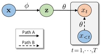
(b) VAE with an auto-regressive decoder

Figure 1: Illustration of learning parameters $\{\boldsymbol{\phi},\boldsymbol{\theta}\}$ in the two different paradigms. Starting from the observation $\boldsymbol{x}$ in blue circle, a VAE infers its latent code $\boldsymbol{z}$ in the green circle, and further generates its reconstruction in the red circle. (a) Standard VAE learning, with only one path via $\{\boldsymbol{\phi},\boldsymbol{\theta}\}$ from $\boldsymbol{x}$ to its reconstruction; (b) VAE learning with an auto-regressive decoder. Two paths are considered from $\boldsymbol{x}$ to its reconstruction: Path A via $\{\boldsymbol{\phi},\boldsymbol{\theta}\}$ and Path B via $\boldsymbol{\theta}$.

3 Cyclical Annealing Schedule

3.1 Identifying Sources of KL Vanishing

In the traditional VAE Kingma and Welling (2013), $\boldsymbol{z}$ generates $\boldsymbol{x}$ directly, and the reconstruction depends only on one path of $\{\boldsymbol{\phi},\boldsymbol{\theta}\}$ passing through $\boldsymbol{z}$, as shown in Figure 1(a). Hence, $\boldsymbol{z}$ can largely determine the reconstructed $\boldsymbol{x}$. In contrast, when an auto-regressive decoder is used in a text VAE Bowman et al. (2015), there are two paths from $\boldsymbol{x}$ to its reconstruction, as shown in Figure 1(b). Path A is the same as that in the standard VAE, where $\boldsymbol{z}$ is the global representation that controls the generation of $\boldsymbol{x}$; Path B leaks the partial ground-truth information of $\boldsymbol{x}$ at every time step of the sequential decoding. It generates $x_{t}$ conditioned on $x_{<t}$. Therefore, Path B can potentially bypass Path A to generate $\boldsymbol{x}$, leading to KL vanishing.

From this perspective, we hypothesize that the model-collapse problem is related to the low quality of $\boldsymbol{z}$ at the beginning phase of decoder training. A lower quality $\boldsymbol{z}$ introduces more difficulties in reconstructing $\boldsymbol{x}$ via Path A. As a result, the model is forced to learn an easier solution to decoding: generating $\boldsymbol{x}$ via Path B only.

We argue that this phenomenon can be easily observed due to the powerful representation capability of the auto-regressive decoder. It has been shown empirically that auto-regressive decoders are able to capture highly-complex distributions, such as natural language sentences Mikolov et al. (2010). This means that Path B alone has enough capacity to model $\boldsymbol{x}$, even though the decoder takes $\{x_{<t},\boldsymbol{z}\}$ as input to produce $x_{t}$. Zhang et al. (2017a) has shown that flexible deep neural networks can easily fit randomly labeled training data, and here the decoder can learn to rely solely on $x_{<t}$ for generation, when $\boldsymbol{z}$ is of low quality.

We use our hypothesis to explain the learning behavior of different scheduling schemes for $\beta$ as follows.

Constant Schedule

The two loss terms in (2) are weighted equally in the constant schedule. At the early stage of optimization, $\{\boldsymbol{\phi},\boldsymbol{\theta}\}$ are randomly initialized and the latent codes $\boldsymbol{z}$ are of low quality. The KL term $\mathcal{L}_{R}$ pushes $q_{\boldsymbol{\phi}}(\boldsymbol{z}|\boldsymbol{x})$ close to an uninformative prior $p(\boldsymbol{z})$: the posterior becomes more like an isotropic Gaussian noise, and less representative of their corresponding observations. In other words, $\mathcal{L}_{R}$ blocks Path A, and thus $\boldsymbol{z}$ remains uninformative during the entire training process: it starts with random initialization and then is regularized towards a random noise. Although the reconstruction term $\mathcal{L}_{E}$ can be satisfied via two paths, since $\boldsymbol{z}$ is noisy, the decoder learns to discard Path A (i.e., ignores $\boldsymbol{z}$), and chooses Path B to generate the sentence word-by-word.

Monotonic Annealing Schedule

The monotonic schedule sets $\beta$ close to $0$ in the early stage of training, which effectively removes the blockage $\mathcal{L}_{R}$ on Path A, and the model reduces to a denoising autoencoder . $\mathcal{L}_{E}$ becomes the only objective, which can be reached by both paths. Though randomly initialized, $\boldsymbol{z}$ is learned to capture useful information for reconstruction of $\boldsymbol{x}$ during training. At the time when the full VAE objective is considered ($\beta=1$), $\boldsymbol{z}$ learned earlier can be viewed as the VAE initialization; such latent variables are much more informative than random, and thus are ready for the decoder to use.

To mitigate the KL-vanishing issue, it is key to have meaningful latent codes $\boldsymbol{z}$ at the beginning of training the decoder, so that $\boldsymbol{z}$ can be utilized. The monotonic schedule under-weights the prior regularization, and the learned $q_{\boldsymbol{\phi}}(\boldsymbol{z}|\boldsymbol{x})$ tends to collapse into a point estimate (i.e., the VAE reduces to an AE). This underestimate can result in sub-optimal decoder learning. A natural question concerns how one can get a better distribution estimate for $\boldsymbol{z}$ as initialization, while retaining low computational cost.

3.2 Cyclical Annealing Schedule

Our proposal is to use $\boldsymbol{z}\sim q_{\boldsymbol{\phi}}(\boldsymbol{z}|\boldsymbol{x})$, which has been trained under the full VAE objective, as initialization. To learn to progressively improve latent representation $\boldsymbol{z}$, we propose a cyclic annealing schedule. We start with $\beta=0$, increase $\beta$ at a fast pace, and then stay at $\beta=1$ for subsequent learning iterations. This encourages the model to converge towards the VAE objective, and infers its first raw full latent distribution.

Unfortunately, Path A is blocked at $\beta=1$. The optimization is then continued at $\beta=0$ again, which perturbs the VAE objective, dislodges it from the convergence, and reopens Path A. Importantly, the decoder is now trained with the latent code from a full distribution $\boldsymbol{z}\sim q_{\boldsymbol{\phi}}(\boldsymbol{z}|\boldsymbol{x})$, and both paths are considered. We repeat this process several times to achieve better convergences.

Formally, $\beta$ has the form:

$$\beta_{t}=\left\{\begin{matrix}f(\tau),&\tau\leq R\\ 1,&\tau>R\end{matrix}\right.~{}~{}~{}\text{with}~{}~{}$$ (6)

$$\tau=\frac{\bmod(t-1,\left\lceil T/M\right\rceil)}{T/M}~{},$$ (7)

where $t$ is the iteration number, $T$ is the total number of training iterations, $f$ is a monotonically increasing function, and we introduce two new hyper-parameters associated with the cyclical annealing schedule:

• $M$: number of cycles (default $M=4$);

• $R$: proportion used to increase $\beta$ within a cycle (default $R=0.5$).

Figure 2: Comparison between (a) traditional monotonic and (b) proposed cyclical annealing schedules.In this figure, $M=4$ cycles are illustrated, $R=0.5$ is used for increasing within each cycle.

In other words, we split the training process into $M$ cycles, each starting with $\beta=0$ and ending with $\beta=1$. We provide an example of a cyclical schedule in Figure 2(b), compared with the monotonic schedule in Figure 2(a). Within one cycle, there are two consecutive stages (divided by $R$):

• Annealing.  $\beta$ is annealed from $0$ to $1$ in the first $R\left\lceil T/M\right\rceil$ training steps over the course of a cycle. For example, the steps $[1,5K]$ in the Figure 2(b). $\beta=f(0)=0$ forces the model to learn representative $\boldsymbol{z}$ to reconstruct $\boldsymbol{x}$. As depicted in Figure 1(b), there is no interruption from the prior on Path A, $\boldsymbol{z}$ is forced to learn the global representation of $\boldsymbol{x}$. By gradually increasing $\beta$ towards $f(R)=1$, $q(\boldsymbol{z}|\boldsymbol{x})$ is regularized to transit from a point estimate to a distribution estimate, spreading out to match the prior.

• Fixing.  As our ultimate goal is to learn a VAE model, we fix $\beta=1$ for the rest of training steps within one cycle, e.g., the steps $[5K,10K]$ in Figure 2(b). This drives the model to optimize the full VAE objective until convergence.

As illustrated in Figure 2, the monotonic schedule increasingly anneals $\beta$ from 0 to 1 once, and fixes $\beta=1$ during the rest of training. The cyclical schedules alternatively repeats the annealing and fixing stages multiple times.

A Practical Recipe

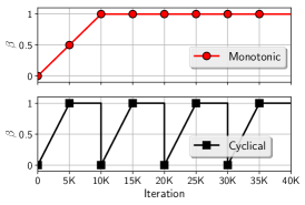
(a) Linear	(b) Sigmoid	(c) Cosine

Figure 7: Comparison between traditional monotonic and proposed cyclical annealing schedules. The top row shows the traditional monotonic schedules, and the bottom row shows their corresponding cyclical schedules. $M=4$ cycles are illustrated, $R=0.5$ is used for annealing within each cycle.

The existing schedules can be viewed as special cases of the proposed cyclical schedule. The cyclical schedule reduces to the constant schedule when $R=0$, and it reduces to an monotonic schedule when $M=1$ and $R$ is relatively small . In theory, any monotonically increasing function $f$ can be adopted for the cyclical schedule, as long as $f(0)=0$ and $f(R)=1$. In practice, we suggest to build the cyclical schedule upon the success of monotonic schedules: we adopt the same $f$, and modify it by setting $M$ and $R$ (as default). Three widely used increasing functions for $f$ are linear Fraccaro et al. (2016); Goyal et al. (2017), Sigmoid Bowman et al. (2015) and Consine Lai et al. (2018). We present the comparative results using the linear function $f(\tau)=\tau/R$ in Figure 2, and show the complete comparison for other functions in Figure 7 of the Supplementary Material (SM).

3.3 On the impact of $\beta$

This section derives a bound for the training objective to rigorously study the impact of $\beta$; the proof details are included in SM. For notational convenience, we identify each data sample with a unique integer index $n\sim q(n)$, drawn from a uniform random variable on $\{1,2,\cdots,N\}$. Further we define $q(\boldsymbol{z}|n)=q_{\boldsymbol{\phi}}(\boldsymbol{z}|\boldsymbol{x}_{n})$ and $q(\boldsymbol{z},n)=q(\boldsymbol{z}|n)q(n)=q(\boldsymbol{z}|n)\frac{1}{N}$. Following Makhzani et al. (2016), we refer to $q(\boldsymbol{z})=\sum_{n=1}^{N}q(\boldsymbol{z}|n)q(n)$ as the aggregated posterior. This marginal distribution captures the aggregated $\boldsymbol{z}$ over the entire dataset. The KL term in (5) can be decomposed into two refined terms Chen et al. (2018); Hoffman and Johnson (2016):

$$\mathcal{F}_{R} =\mathbb{E}_{q(n)}[\mbox{KL}(q(\boldsymbol{z}|n)||p(\boldsymbol{z}))]$$

$$=\underbrace{I_{q}(\boldsymbol{z},n)}_{\mathcal{F}_{1}:~{}\text{Mutual~{}Info.}}+\underbrace{\mbox{KL}(q(\boldsymbol{z})||p(\boldsymbol{z}))}_{\mathcal{F}_{2}:~{}\text{Marginal KL}}$$ (8)

where $\mathcal{F}_{1}$ is the mutual information (MI) measured by $q$. Higher MI can lead to a higher correlation between the latent variable and data variable, and encourages a reduction in the degree of KL vanishing. The marginal KL is represented by $\mathcal{F}_{2}$, and it measures the fitness of the aggregated posterior to the prior distribution.

The reconstruction term in (5) provides a lower bound for MI measured by $q$, based on Corollary 3 in Li et al. (2017):

$$\mathcal{F}_{E} =E_{q(n),\boldsymbol{z}\sim q(\boldsymbol{z}|n)}(\log p(n|\boldsymbol{z}))]+H_{q}(n)$$

$$\leq I_{q}(\boldsymbol{z},n)$$ (9)

where $H(n)$ is a constant.

Analysis of $\beta$

When scheduled with $\beta$, the training objective over the dataset can be written as:

$$\mathcal{F} =-\mathcal{F}_{E}+\beta\mathcal{F}_{R}$$ (10)

$$\geq(\beta-1)I_{q}(\boldsymbol{z},n)+\beta\mbox{KL}(q(\boldsymbol{z})||p(\boldsymbol{z}))$$ (11)

To reduce KL vanishing, we desire an increase in the MI term $I(\boldsymbol{z},n)$, which appears in both $\mathcal{F}_{E}$ and $\mathcal{F}_{R}$, modulated by $\beta$. It shows that reducing KL vanishing is inversely proportional with $\beta$. When $\beta=0$, the model fully focuses on maximizing the MI. As $\beta$ increases, the model gradually transits towards fitting the aggregated latent codes to the given prior. When $\beta=1$, the implementation of MI becomes implicit in $\mbox{KL}(q(\boldsymbol{z})||p(\boldsymbol{z}))$. It is determined by the amortized inference regularization (implied by the encoder’s expressivity) Shu et al. (2018), which further affects the performance of the generative density estimator.

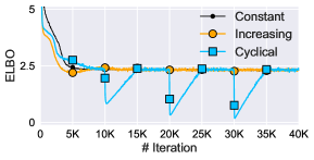
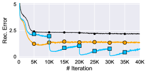
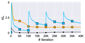
(a) ELBO	(b) Reconstruction Error	(c) KL term

Figure 3: Comparison of the learning curves for the three schedules on an illustrative problem.

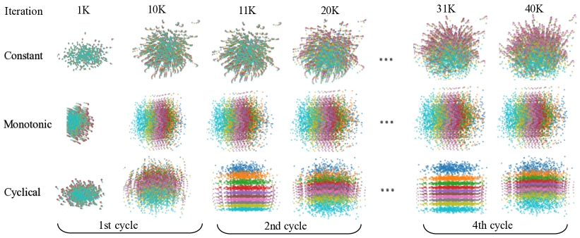
Figure 4: Visualization of the latent space along the learning dynamics on an illustrative problem.

4 Visualization of Latent Space

We compare different schedule methods by visualizing the learning processes on an illustrative problem. Consider a dataset consisting of 10 sequences, each of which is a 10-dimensional one-hot vector with the value 1 appearing in different positions. A 2-dimensional latent space is used for the convenience of visualization. Both the encoder and decoder are implemented using a 2-layer LSTM with 64 hidden units each. We use $T\!=\!40$K total iterations, and the scheduling schemes in Figure 2.

The learning curves for the ELBO, reconstruction error, and KL term are shown in Figure 3. The three schedules share very similar values. However, the cyclical schedule provides substantially lower reconstruction error and higher KL divergence. Interestingly, the cyclical schedule improves the performance progressively: it becomes better than the previous cycle, and there are clear periodic patterns across different cycles. This suggests that the cyclical schedule allows the model to use the previously learned results as a warm-restart to achieve further improvement.

We visualize the resulting division of the latent space for different training steps in Figure 4, where each color corresponds to $\boldsymbol{z}\sim q(\boldsymbol{z}|n)$, for $n=1,\cdots,10$. We observe that the constant schedule produces heavily mixed latent codes $\boldsymbol{z}$ for different sequences throughout the entire training process. The monotonic schedule starts with a mixed $\boldsymbol{z}$, but soon divides the space into a mixture of 10 cluttered Gaussians in the annealing process (the division remains cluttered in the rest of training). The cyclical schedule behaves similarly to the monotonic schedule in the first 10K steps (the first cycle). But, starting from the 2nd cycle, much more divided clusters are shown when learning on top of the 1st cycle results. However, $\beta<1$ leads to some holes between different clusters, making $q(\boldsymbol{z})$ violate the constraint of $p(\boldsymbol{z})$. This is alleviated at the end of the 2nd cycle, as the model is trained with $\beta=1$. As the process repeats, we see clearer patterns in the 4th cycle than the 2nd cycle for both $\beta<0$ and $\beta=1$. It shows that more structured information is captured in $\boldsymbol{z}$ using the cyclical schedule, which is beneficial in downstream applications as shown in the experiments.

5 Related Work

Solutions to KL vanishing

Several techniques have been proposed to mitigate the KL vanishing issue. The proposed method is most closely related to the monotonic KL annealing technique in Bowman et al. (2015). In addition to introducing a specific algorithm, we have comprehensively studied the impact of $\beta$ and its scheduling schemes. Our explanations can be used to interpret other techniques, which can be broadly categorized into two classes.

The first category attempts to weaken Path B, and force the decoder to use Path A. Word drop decoding Bowman et al. (2015) sets a certain percentage of the target words to zero. It has shown that it may degrade the performance when the drop rate is too high. The dilated CNN was considered in Yang et al. (2017) as a new type of decoder to replace the LSTM. By changing the decoder’s dilation architecture, one can control Path B: the effective context from $x_{<t}$.

The second category of techniques improves the dependency in Path A, so that the decoder uses latent codes more easily. Skip connections were developed in Dieng et al. (2018) to shorten the paths from $\boldsymbol{z}$ to $\boldsymbol{x}$ in the decoder. Zhao et al. (2017) introduced an auxiliary loss that requires the decoder to predict the bag-of-words in the dialog response Zhao et al. (2017). The decoder is thus forced to capture global information about the target response.  Zhao et al. (2019) enhanced Path A via mutual information. Concurrent with our work, He et al. (2019) proposed to update encoder multiple times to achieve better latent code before updating decoder. Semi-amortized training Kim et al. (2018) was proposed to perform stochastic variational inference (SVI) Hoffman et al. (2013) on top of the amortized inference in VAE. It shares a similar motivation with the proposed approach, in that better latent codes can reduce KL vanishing. However, the computational cost to run SVI is high, while our monotonic schedule does not require any additional compute overhead. The KL scheduling methods are complementary to these techniques. As shown in experiments, the proposed cyclical schedule can further improve them.

$\beta$-VAE

The VAE has been extended to $\beta$-regularized versions in a growing body of work Higgins et al. (2017); Alemi et al. (2018). Perhaps the seminal work is $\beta$-VAE Higgins et al. (2017), which was extended in  Kim and Mnih (2018); Chen et al. (2018) to consider $\beta$ on the refined terms in the KL decomposition. Their primary goal is to learn disentangled latent representations to explain the data, by setting $\beta>1$. From an information-theoretic point of view, (Alemi et al., 2018) suggests a simple method to set $\beta<1$ to ensure that latent-variable models with powerful stochastic decoders do not ignore their latent code. However, $\beta\neq 1$ results in an improper statistical model. Further, $\beta$ is static in their work; we consider dynamically scheduled $\beta$ and find it more effective.

Cyclical schedules

Warm-restart techniques are common in optimization to deal with multimodal functions. The cyclical schedule has been used to train deep neural networks Smith (2017), warm restart stochastic gradient descent Loshchilov and Hutter (2017), improve convergence rates Smith and Topin (2017), obtain model ensembles Huang et al. (2017) and explore multimodal distributions in MCMC sampling Zhang et al. (2019). All these works applied cyclical schedules to the learning rate. In contrast, this paper represents the first to consider the cyclical schedule for $\beta$ in VAE. Though the techniques seem simple and similar, our motivation is different: we use the cyclical schedule to re-open Path A in Figure 1(b) and provide the opportunity to train the decoder with high-quality $\boldsymbol{z}$.

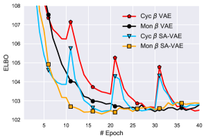
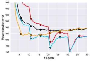
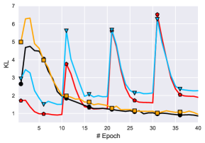
(a) ELBO	(b) Reconstruction error	(c) KL

Figure 5: Learning curves of VAE and SA-VAE on PTB. Under similar ELBO, the cyclical schedule provides lower reconstruction errors and higher KL values than the monotonic schedule.

6 Experiments

The source code to reproduce the experimental results will be made publicly available on GitHub. For a fair comparison, we follow the practical recipe described in Section 3.2, where the monotonic schedule is treated as a special case of cyclical schedule (while keeping all other settings the same). The default hyper-parameters of the cyclical schedule are used in all cases unless stated otherwise. We study the impact of hyper-parameters in the SM, and show that larger $M$ can provide higher performance for various $R$. We show the major results in this section, and put more details in the SM. The monotonic and cyclical schedules are denoted as M and C, respectively.

6.1 Language Modeling

We first consider language modeling on the Penn Tree Bank (PTB) dataset Marcus et al. (1993). Language modeling with VAEs has been a challenging problem, and few approaches have been shown to produce rich generative models that do not collapse to standard language models. Ideally a deep generative model trained with variational inference would pursue higher ELBO, making use of the latent space (i.e., maintain a nonzero KL term) while accurately modeling the underlying distribution (i.e., lower reconstruction errors). We implemented different schedules based on the code published by Kim et al. (2018).

Table 1: Comparison of language modeling on Penn Tree Bank (PTB). The last iteration results are reported. Since SA-VAE tends to overfit, we report its best results in row M^∗.

Table 2: Generated dialog responses from the cyclical and monotonic schedules.

The latent variable is 32-dimensional, and 40 epochs are used. We compare the proposed cyclical annealing schedule with the monotonic schedule baseline that, following Bowman et al. (2015), anneals linearly from 0 to 1.0 over 10 epochs. We also compare with semi-amortized (SA) training Kim et al. (2018), which is considered as the state-of-the-art technique in preventing KL vanishing. We set SVI steps to 10.

Results are shown in Table 1. The perplexity is reported in column PPL. The cyclical schedule outperforms the monotonic schedule for both standard VAE and SA-VAE training. SA-VAE training can effectively reduce KL vanishing, it takes 472s per epoch. However, this is significantly more expensive than the standard VAE training which takes 30s per epoch. The proposed cyclical schedule adds almost zero cost.

We show the learning curves for VAE and SA-VAE in Figure 5. Interestingly, the cyclical schedule exhibits periodical learning behaviours. The performance of the cyclical schedule gets better progressively, after each cycle. While ELBO and PPL ar similar, the cyclical schedule improves the reconstruction ability and KL values for both VAE and SA-VAE. We observe clear over-fitting issues for the SA-VAE with the monotonic schedule, while this issue is less severe for SA-VAE with the cyclical schedule.

Finally, we further investigate whether our improvements are from simply having a lower $\beta$, rather than from the cyclical schedule re-opening Path A for better learning. To test this, we use a monotonic schedule with maximum $\beta=0.5$. We observe that the reconstruction and KL terms perform better individually, but the ELBO is substantially worse than $\beta=1$, because $\beta=0.5$ yields an improper model. Even so, the cyclical schedule improves its performance.

Model	CVAE		CVAE+BoW
Schedule	M	C	M	C
Rec-P $\downarrow$	36.16	29.77	18.44	16.74
KL Loss $\uparrow$	0.265	4.104	14.06	15.55
B4 prec	0.185	0.234	0.211	0.219
B4 recall	0.122	0.220	0.210	0.219
A-bow prec	0.957	0.961	0.958	0.961
A-bow recall	0.911	0.941	0.938	0.940
E-bow prec	0.867	0.833	0.830	0.828
E-bow recall	0.784	0.808	0.808	0.805

Table 3: Comparison on dialog response generation. Reconstruction perplexity (Rec-P) and BLEU (B) scores are used for evaluation.

6.2 Conditional VAE for Dialog

We use a cyclical schedule to improve the latent codes in Zhao et al. (2017), which are key to diverse dialog-response generation. Following Zhao et al. (2017), Switchboard (SW) Corpus Godfrey and Holliman (1997) is used, which has 2400 two-sided telephone conversations.

Two latent variable models are considered. The first one is the Conditional VAE (CVAE), which has been shown better than the encoder-decoder neural dialog Serban et al. (2016). The second is to augment VAE with a bag-of-word (BoW) loss to tackle the KL vanishing problem, as proposed in Zhao et al. (2017).

Table 2 shows the sample outputs generated from the two schedules using CVAE. Caller $\mathtt{Alice}$ begins with an open-ended statement on choosing a college, and the model learns to generate responses from Caller $\mathtt{Bob}$. The cyclical schedule generated highly diverse answers that cover multiple plausible dialog acts. On the contrary, the responses from the monotonic schedule are limited to repeat plain responses, i.e., “i’m not sure”.

Quantitative results are shown in Table 3, using the evaluation metrics from Zhao et al. (2017). $(\textup{\it i})$ Smoothed Sentence-level BLEU Chen and Cherry (2014): BLEU is a popular metric that measures the geometric mean of modified n-gram precision with a length penalty. We use BLEU-1 to 4 as our lexical similarity metric and normalize the score to 0 to 1 scale. $(\textup{\it ii})$ Cosine Distance of Bag-of-word Embedding Liu et al. (2016): a simple method to obtain sentence embeddings is to take the average or extreme of all the word embeddings in the sentences. We used Glove embedding and denote the average method as A$-$bow and extreme method as E$-$bow. The score is normalized to $[0,1]$. Higher values indicate more plausible responses.

The BoW indeed reduces the KL vanishing issue, as indicated by the increased KL and decreased reconstruction perplexity. When applying the proposed cyclical schedule to CVAE, we also see a reduced KL vanishing issue. Interestingly, it also yields the highest BLEU scores. This suggests that the cyclical schedule can generate dialog responses of higher fidelity with lower cost, as the auxiliary BoW loss is not necessary. Further, BoW can be improved when integrated with the cyclical schedule, as shown in the last column of Table 3.

6.3 Unsupervised Language Pre-training

We consider the Yelp dataset, as pre-processed in Shen et al. (2017) for unsupervised language pre-training. Text features are extracted as the latent codes $\boldsymbol{z}$ of VAE models, pre-trained with monotonic and cyclical schedules. The AE is used as the baseline. A good VAE can learn to cluster data into meaningful groups Kingma and Welling (2013), indicating that well-structured $\boldsymbol{z}$ are highly informative features, which usually leads to higher classification performance. To clearly compare the quality of $\boldsymbol{z}$, we build a simple one-layer classifier on $\boldsymbol{z}$, and fine-tune the model on different proportions of labelled data Zhang et al. (2017b).

The results are shown in Figure 6. The cyclical schedule consistently yields the highest accuracy relative to other methods. We visualize the tSNE embeddings Maaten and Hinton (2008) of $\boldsymbol{z}$ in Figure 9 of the SM, and observe that the cyclical schedule exhibits clearer clustered patterns.

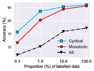
Figure 6: Accuracy of fine-tuning on the unsupervised pre-trained models on the Yelp dataset.

Schedule	Rec	KL	ELBO
Cyc $\beta$ + Const $\eta$	101.30	1.457	-102.76
Mon $\beta$ + Const $\eta$	101.93	0.858	-102.78
Cyc $\beta$ + Cyc $\eta$	100.61	1.897	-102.51
Mon $\beta$ + Cyc $\eta$	101.74	0.748	-102.49

Table 4: Comparison of cyclical schedules on $\beta$ and $\eta$, tested with language modeling on PTB.

6.4 Ablation Study

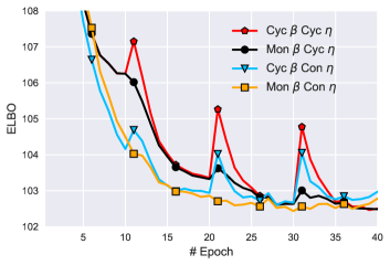
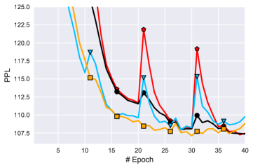
(a) ELBO	(b) PPL
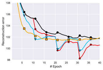
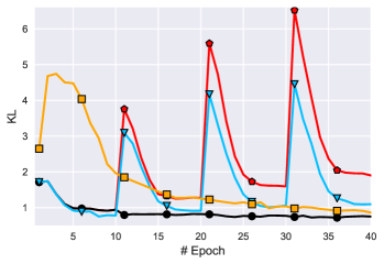
(c) Reconstruction error	(d) KL

Figure 10: Ablation study on cyclical schedules on $\beta$ and $\eta$.

To enhance the performance, we propose to apply the cyclical schedule to the learning rate $\eta$ on real tasks. It ensures that the optimizer has the same length of optimization trajectory for each $\beta$ cycle (so that each cycle can fully converge). To investigate the impact of cyclical on $\eta$, we perform two more ablation experiments: $(\textup{\it i})$ We make only $\beta$ cyclical, keep $\eta$ constant. $(\textup{\it ii})$ We make only $\eta$ cyclical, keep $\beta$ monotonic. The last epoch numbers are shown in Table 4, and the learning curves on shown in Figure 10 in SM. Compared with the baseline, we see that it is the cyclical $\beta$ rather than cyclical $\eta$ that contributes to the improved performance.

7 Conclusions

We provide a novel two-path interpretation to explain the KL vanishing issue, and identify its source as a lack of good latent codes at the beginning of decoder training. This provides an understanding of various $\beta$ scheduling schemes, and motivates the proposed cyclical schedule. By re-opening the path at $\beta=0$, the cyclical schedule can progressively improve the performance, by leveraging good latent codes learned in the previous cycles as warm re-starts. We demonstrate the effectiveness of the proposed approach on three NLP tasks, and show that it is superior to or complementary to other techniques.

Appendix A Comparison of different schedules

We compare the two different scheduling schemes in Figure 7. The three widely used monotonic schedules are shown in the top row, including linear, sigmoid and cosine. We can easily turn them into their corresponding cyclical versions, shown in the bottom row.

Appendix B Proofs on the $\beta$ and MI

When scheduled with $\beta$, the training objective over the dataset can be written as:

$$\mathcal{F} =-\mathcal{F}_{E}+\beta\mathcal{F}_{R}$$ (12)

We proceed the proof by re-writing each term separately.

B.1 Bound on $\mathcal{F}_{E}$

Following Li et al. (2017), on the support of $(\boldsymbol{x},\boldsymbol{z})$, we denote $q$ as the encoder probability measure, and $p$ as the decoder probability measure. Note that the reconstruction loss for $\boldsymbol{z}$ can be writen as its negative log likelihood form as:

$$\mathcal{F}_{E}=-\mathbb{E}_{\boldsymbol{x}\sim q(\boldsymbol{x}),\boldsymbol{z}\sim q(\boldsymbol{z}|\boldsymbol{x})}[\log p(\boldsymbol{x}|\boldsymbol{z})].$$ (13)

Lemma 1

For random variables $\boldsymbol{x}$ and $\boldsymbol{z}$ with two different probability measures, $p(\boldsymbol{x},\boldsymbol{z})$ and $q(\boldsymbol{x},\boldsymbol{z})$, we have

$$H_{p}(\boldsymbol{z}|\boldsymbol{x})$$

$$=-\mathbb{E}_{\boldsymbol{z}\sim p(\boldsymbol{z}),x\sim p(\boldsymbol{x}|\boldsymbol{z})}[\log p(\boldsymbol{z}|\boldsymbol{x})]$$

$$=-\mathbb{E}_{\boldsymbol{z}\sim p(\boldsymbol{z}),\boldsymbol{x}\sim p(\boldsymbol{x}|\boldsymbol{z})}[\log q(\boldsymbol{z}|\boldsymbol{x})]$$

$$-\mathbb{E}_{\boldsymbol{z}\sim p(\boldsymbol{z}),x\sim p(\boldsymbol{x}|\boldsymbol{z})}\big{[}\log p(\boldsymbol{z}|\boldsymbol{x})-\log q(\boldsymbol{z}|\boldsymbol{x})\big{]}$$

$$=-\mathbb{E}_{\boldsymbol{z}\sim p(\boldsymbol{z}),\boldsymbol{x}\sim p(\boldsymbol{x}|\boldsymbol{z})}[\log q(\boldsymbol{z}|\boldsymbol{x})]$$

$$-\mathbb{E}_{p(\boldsymbol{x})}(\mbox{KL}(p(\boldsymbol{z}|\boldsymbol{x})\|q(\boldsymbol{z}|\boldsymbol{x})))$$

$$\leq-\mathbb{E}_{\boldsymbol{z}\sim p(\boldsymbol{z}),\boldsymbol{x}\sim p(\boldsymbol{x}|\boldsymbol{z})}[\log q(\boldsymbol{z}|\boldsymbol{x})]$$ (14)

where $H_{p}(\boldsymbol{z}|\boldsymbol{x})$ is the conditional entropy. Similarly, we can prove that

$$H_{q}(\boldsymbol{x}|\boldsymbol{z})\leq-\mathbb{E}_{\boldsymbol{x}\sim q(\boldsymbol{x}),\boldsymbol{z}\sim q(\boldsymbol{z}|\boldsymbol{x})}[\log p(\boldsymbol{x}|\boldsymbol{z})]$$ (15)

From lemma 1, we have

Corollary 1

For random variables $\boldsymbol{x}$ and $\boldsymbol{z}$ with probability measure $p(\boldsymbol{x},\boldsymbol{z})$, the mutual information between $\boldsymbol{x}$ and $\boldsymbol{z}$ can be written as

$$I_{q}(\boldsymbol{x},\boldsymbol{z}) =H_{q}(\boldsymbol{x})-H_{q}(\boldsymbol{x}|\boldsymbol{z})\geq H_{q}(\boldsymbol{x})$$

$$+\mathbb{E}_{\boldsymbol{x}\sim q(\boldsymbol{x}),\boldsymbol{z}\sim q(\boldsymbol{z}|\boldsymbol{x})}[\log p(\boldsymbol{x}|\boldsymbol{z})]$$

$$=H_{q}(\boldsymbol{x})+\mathcal{F}_{E}$$ (16)

B.2 Decomposition of $\mathcal{F}_{R}$

The KL term in (5) can be decomposed into two refined terms Hoffman and Johnson (2016):

$$\mathcal{F}_{R}$$

$$=\mathbb{E}_{q(\boldsymbol{x})}[\mbox{KL}(q(\boldsymbol{z}|\boldsymbol{x})||p(\boldsymbol{z}))]$$

$$=\mathbb{E}_{q(\boldsymbol{z},\boldsymbol{x})}[(\log q(\boldsymbol{z}|\boldsymbol{x})-\log p(\boldsymbol{z}))]$$

$$=\mathbb{E}_{q(\boldsymbol{z},\boldsymbol{x})}[(\log q(\boldsymbol{z}|\boldsymbol{x})-\log q(\boldsymbol{z})]$$

$$\hskip 28.45274pt+\mathbb{E}_{q(\boldsymbol{z},\boldsymbol{x})}[\log q(\boldsymbol{z})-\log p(\boldsymbol{z}))]$$

$$=\mathbb{E}_{q(\boldsymbol{z},\boldsymbol{x})}[(\log q(\boldsymbol{z},\boldsymbol{x})-\log q(\boldsymbol{x})-\log q(\boldsymbol{z})]$$

$$\hskip 28.45274pt+\mathbb{E}_{q(\boldsymbol{z},\boldsymbol{x})}[\log q(\boldsymbol{z})-\log p(\boldsymbol{z}))]$$

$$=\underbrace{I_{q}(\boldsymbol{z},\boldsymbol{x})}_{\mathcal{F}_{1}:~{}\text{Mutual~{}Info.}}+\underbrace{\mbox{KL}(q(\boldsymbol{z})||p(\boldsymbol{z}))}_{\mathcal{F}_{2}:~{}\text{Marginal KL}}$$ (17)

Appendix C Model Description

C.1 Conditional VAE for dialog

Each conversation can be represented via three random variables: the dialog context ${\boldsymbol{c}}$ composed of the dialog history, the response utterance $\boldsymbol{x}$, and a latent variable $\boldsymbol{z}$, which is used to capture the latent distribution over the valid responses($\beta=1$) Zhao et al. (2017). The ELBO can be written as:

$$\log p_{\boldsymbol{\theta}}(\boldsymbol{x}|{\boldsymbol{c}}) \geq\mathcal{L}_{\text{ELBO}}$$ (18)

$$=\mathbb{E}_{q_{\boldsymbol{\phi}}(\boldsymbol{z}|\boldsymbol{x},{\boldsymbol{c}})}\big{[}\log p_{\boldsymbol{\theta}}(\boldsymbol{x}|\boldsymbol{z},{\boldsymbol{c}})\big{]}$$

$$-\beta\mbox{KL}(q_{\boldsymbol{\phi}}(\boldsymbol{z}|\boldsymbol{x},{\boldsymbol{c}})||p(\boldsymbol{z}|{\boldsymbol{c}}))$$

C.2 Semi-supervised learning with VAE

We use a simple factorization to derive the ELBO for semi-supervised learning. $\alpha$ is introduced to regularize the strength of classification loss.

$$\log p_{\boldsymbol{\theta}}(\boldsymbol{y},\boldsymbol{x})\geq\mathcal{L}_{\text{ELBO}}$$ (19)

$$=\mathbb{E}_{q_{\boldsymbol{\phi}}(\boldsymbol{z}|\boldsymbol{x})}\big{[}\log p_{\boldsymbol{\theta}}(\boldsymbol{x}|\boldsymbol{z})+\alpha\log p_{\boldsymbol{\psi}}(\boldsymbol{y}|\boldsymbol{z})\big{]}$$

$$-\beta\mbox{KL}(q_{\boldsymbol{\phi}}(\boldsymbol{z}|\boldsymbol{x})||p(\boldsymbol{z}))$$ (20)

where $\boldsymbol{\psi}$ is the parameters for the classifier.

Good latent codes $\boldsymbol{z}$ are crucial for the the classification performance, especially when simple classifiers are employed, or less labelled data is available.

Appendix D More Experimental Results

D.1 CVAE for Dialog Response Generation

Code $\&$ Dataset

We implemented different schedules based on the code published by Zhao et al. (2017). In the SW dataset, there are 70 available topics. We randomly split the data into 2316/60/62 dialogs for train/validate/test.

Results

The results on full BLEU scores are shown in Table 5. The cyclical schedule outperforms the monotonic schedule in both settings. The learning curves are shown in Figure 8. Under similar ELBO results, the cyclical schedule provide lower reconstruction errors, higher KL values, and higher BLEU values than the monotonic schedule. Interestingly, the monotonic schedule tends to overfit, while the cyclical schedule does not, particularly on reconstruction errors. It means the monotonic schedule can learn better latent codes for VAEs, thus preventing overfitting.

D.2 Semi-supervised Text Classification

Dataset

Yelp restaurant reviews dataset utilizes user ratings associated with each review. Reviews with rating above three are considered positive, and those below three are considered negative. Hence, this is a binary classification problem. The pre-processing in Shen et al. (2017) allows sentiment analysis on sentence level. It further filters the sentences by eliminating those that exceed 15 words. The resulting dataset has 250K negative sentences, and 350K positive ones. The vocabulary size is 10K after replacing words occurring less than 5 times with the “$<$unk$>$” token.

Results

The tSNE embeddings are visualized in Figure 9. We see that cyclical $\beta$ provides much more separated latent structures than the other two methods.

D.3 Hyper-parameter tuning

The cyclical schedule has two hyper-parameters $M$ and $R$. We provide the full results on $M$ and $R$ in Figure 11 and Figure 12, respectively. A larger number of cycles $M$ can provide higher performance for various proportion value $R$.

Model	CVAE		CVAE+BoW
Schedule	M	C	M	C
B1 prec	0.326	0.423	0.384	0.397
B1 recall	0.214	0.391	0.376	0.387
B2 prec	0.278	0.354	0.320	0.331
B2 recall	0.180	0.327	0.312	0.323
B3 prec	0.237	0.299	0.269	0.279
B3 recall	0.153	0.278	0.265	0.275
B4 prec	0.185	0.234	0.211	0.219
B4 recall	0.122	0.220	0.210	0.219

Table 5: Comparison on dialog response generation. BLEU (B) scores 1-4 are used for evaluation. Monotonic (M) and Cyclical (C) schedules are tested on two models.

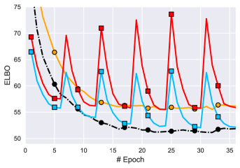
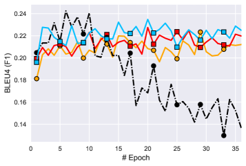
(a) ELBO	(b) BLEU-4 (F1)
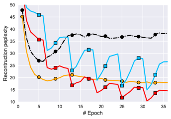
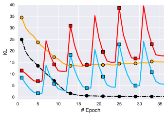
(c) Reconstruction error	(d) KL

Figure 8: Full results of CVAE and BoW+CVAE on SW dataset. Under similar ELBO results, the cyclical schedule provide lower reconstruction errors, higher KL values, and higher BLEU values than the monotonic schedule. Interestingly, the monotonic schedule tends to overfit, while the cyclical schedule does not.

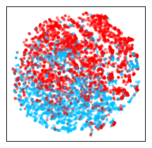
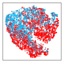
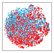
(a) Cyclical $\beta$ VAE	(b) Monotonic $\beta$ VAE	(c) AE

Figure 9: Comparison of tSNE embeddings for three methods on Yelp dataset. This can be considered as the unsupervised feature learning results in semi-supervised learning. More structured latent patterns usually lead to better classification performance.

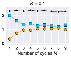
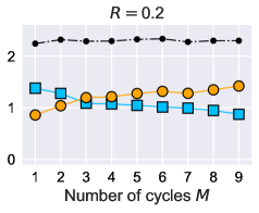
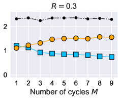
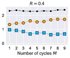
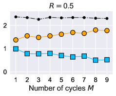
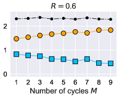
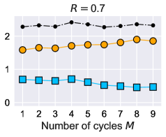
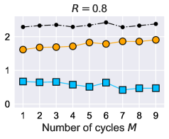
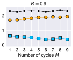
Figure 11: The impact of hyper-parameter $M$: number of cycles. A larger number of cycles lead to better performance. The improvement is more significant when $R$ is small. The improvement is small when $R$ is large.

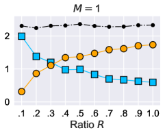
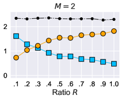
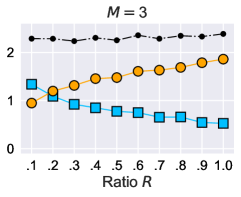
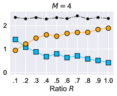
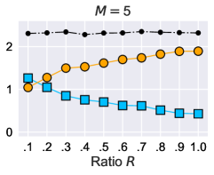
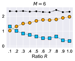
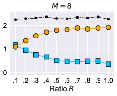
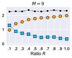
Figure 12: The impact of hyper-parameter $R$: proportion for the annealing stage. A larger $R$ leads to better performance for various $M$. Small $R$ performs worse, because the schedule becomes more similar with constant schedule. $M=1$ recovers the monotonic schedule. Contrary to the convention that typically adopts small $R$, our results suggests that larger $R$ should be considered.

References

- Alemi et al. (2018) Alexander Alemi, Ben Poole, Ian Fischer, Joshua Dillon, Rif A Saurous, and Kevin Murphy. 2018. Fixing a broken ELBO. In ICML.
- Bowman et al. (2015) Samuel R Bowman, Luke Vilnis, Oriol Vinyals, Andrew M Dai, Rafal Jozefowicz, and Samy Bengio. 2015. Generating sentences from a continuous space. arXiv preprint arXiv:1511.06349.
- Chen and Cherry (2014) Boxing Chen and Colin Cherry. 2014. A systematic comparison of smoothing techniques for sentence-level bleu. In Proceedings of the Ninth Workshop on Statistical Machine Translation, pages 362–367.
- Chen et al. (2018) Ricky TQ Chen, Xuechen Li, Roger Grosse, and David Duvenaud. 2018. Isolating sources of disentanglement in VAEs. NIPS.
- Dieng et al. (2018) Adji B Dieng, Yoon Kim, Alexander M Rush, and David M Blei. 2018. Avoiding latent variable collapse with generative skip models. arXiv preprint arXiv:1807.04863.
- Fraccaro et al. (2016) Marco Fraccaro, Søren Kaae Sønderby, Ulrich Paquet, and Ole Winther. 2016. Sequential neural models with stochastic layers. In NIPS.
- Godfrey and Holliman (1997) J Godfrey and E Holliman. 1997. Switchboard-1 release 2: Linguistic data consortium. SWITCHBOARD: A User’s Manual.
- Goodfellow et al. (2016) Ian Goodfellow, Yoshua Bengio, and Aaron Courville. 2016. Deep learning, volume 1. MIT press Cambridge.
- Goyal et al. (2017) Anirudh Goyal Alias Parth Goyal, Alessandro Sordoni, Marc-Alexandre Côté, Nan Rosemary Ke, and Yoshua Bengio. 2017. Z-forcing: Training stochastic recurrent networks. In NIPS.
- He et al. (2019) Junxian He, Daniel Spokoyny, Graham Neubig, and Taylor Berg-Kirkpatrick. 2019. Lagging inference networks and posterior collapse in variational autoencoders. ICLR.
- Higgins et al. (2017) Irina Higgins, Loic Matthey, Arka Pal, Christopher Burgess, Xavier Glorot, Matthew Botvinick, Shakir Mohamed, and Alexander Lerchner. 2017. beta-vae: Learning basic visual concepts with a constrained variational framework. ICLR.
- Hochreiter and Schmidhuber (1997) Sepp Hochreiter and Jurgen Schmidhuber. 1997. Long short-term memory. Neural computation.
- Hoffman et al. (2013) Matthew D Hoffman, David M Blei, Chong Wang, and John Paisley. 2013. Stochastic variational inference. The Journal of Machine Learning Research.
- Hoffman and Johnson (2016) Matthew D Hoffman and Matthew J Johnson. 2016. Elbo surgery: yet another way to carve up the variational evidence lower bound. In Workshop in Advances in Approximate Bayesian Inference, NIPS.
- Hu et al. (2017) Zhiting Hu, Zichao Yang, Xiaodan Liang, Ruslan Salakhutdinov, and Eric P Xing. 2017. Toward controlled generation of text. ICML.
- Huang et al. (2017) Gao Huang, Yixuan Li, Geoff Pleiss, Zhuang Liu, John E Hopcroft, and Kilian Q Weinberger. 2017. Snapshot ensembles: Train 1, get m for free. ICLR.
- Kim and Mnih (2018) Hyunjik Kim and Andriy Mnih. 2018. Disentangling by factorising. ICML.
- Kim et al. (2018) Yoon Kim, Sam Wiseman, Andrew C Miller, David Sontag, and Alexander M Rush. 2018. Semi-amortized variational autoencoders. ICML.
- Kingma and Welling (2013) Diederik P Kingma and Max Welling. 2013. Auto-encoding variational bayes. ICLR.
- Lai et al. (2018) Guokun Lai, Bohan Li, Guoqing Zheng, and Yiming Yang. 2018. Stochastic wavenet: A generative latent variable model for sequential data. ICML workshop.
- Li et al. (2017) Chunyuan Li, Hao Liu, Changyou Chen, Yuchen Pu, Liqun Chen, Ricardo Henao, and Lawrence Carin. 2017. ALICE: Towards understanding adversarial learning for joint distribution matching. In NIPS.
- Liu et al. (2016) Chia-Wei Liu, Ryan Lowe, Iulian V Serban, Michael Noseworthy, Laurent Charlin, and Joelle Pineau. 2016. How not to evaluate your dialogue system: An empirical study of unsupervised evaluation metrics for dialogue response generation. arXiv preprint arXiv:1603.08023.
- Loshchilov and Hutter (2017) Ilya Loshchilov and Frank Hutter. 2017. Sgdr: Stochastic gradient descent with warm restarts. ICLR.
- Maaten and Hinton (2008) Laurens van der Maaten and Geoffrey Hinton. 2008. Visualizing data using t-sne. Journal of machine learning research, 9(Nov):2579–2605.
- Makhzani et al. (2016) Alireza Makhzani, Jonathon Shlens, Navdeep Jaitly, Ian Goodfellow, and Brendan Frey. 2016. Adversarial autoencoders. ICLR workshop.
- Marcus et al. (1993) Mitchell P Marcus, Mary Ann Marcinkiewicz, and Beatrice Santorini. 1993. Building a large annotated corpus of english: The penn treebank. Computational linguistics.
- Miao and Blunsom (2016) Yishu Miao and Phil Blunsom. 2016. Language as a latent variable: Discrete generative models for sentence compression. EMNLP.
- Miao et al. (2016) Yishu Miao, Lei Yu, and Phil Blunsom. 2016. Neural variational inference for text processing. In ICML.
- Mikolov et al. (2010) Tomáš Mikolov, Martin Karafiát, Lukáš Burget, Jan Černockỳ, and Sanjeev Khudanpur. 2010. Recurrent neural network based language model. In Eleventh Annual Conference of the International Speech Communication Association.
- Rezende et al. (2014) Danilo Jimenez Rezende, Shakir Mohamed, and Daan Wierstra. 2014. Stochastic backpropagation and approximate inference in deep generative models. ICML.
- Serban et al. (2016) Iulian Vlad Serban, Alessandro Sordoni, Yoshua Bengio, Aaron C Courville, and Joelle Pineau. 2016. Building end-to-end dialogue systems using generative hierarchical neural network models. In AAAI.
- Shen et al. (2017) Tianxiao Shen, Tao Lei, Regina Barzilay, and Tommi Jaakkola. 2017. Style transfer from non-parallel text by cross-alignment. In NIPS.
- Shu et al. (2018) Rui Shu, Hung H Bui, Shengjia Zhao, Mykel J Kochenderfer, and Stefano Ermon. 2018. Amortized inference regularization. NIPS.
- Smith (2017) Leslie N Smith. 2017. Cyclical learning rates for training neural networks. In WACV. IEEE.
- Smith and Topin (2017) Leslie N Smith and Nicholay Topin. 2017. Super-convergence: Very fast training of residual networks using large learning rates. arXiv preprint arXiv:1708.07120.
- Wen et al. (2017) Tsung-Hsien Wen, Yishu Miao, Phil Blunsom, and Steve Young. 2017. Latent intention dialogue models. ICML.
- Xu et al. (2017) Weidi Xu, Haoze Sun, Chao Deng, and Ying Tan. 2017. Variational autoencoder for semi-supervised text classification. In AAAI.
- Yang et al. (2017) Zichao Yang, Zhiting Hu, Ruslan Salakhutdinov, and Taylor Berg-Kirkpatrick. 2017. Improved variational autoencoders for text modeling using dilated convolutions. ICML.
- Zhang et al. (2017a) Chiyuan Zhang, Samy Bengio, Moritz Hardt, Benjamin Recht, and Oriol Vinyals. 2017a. Understanding deep learning requires rethinking generalization. ICLR.
- Zhang et al. (2019) Ruqi Zhang, Chunyuan Li, Jianyi Zhang, Changyou Chen, and Andrew Gordon Wilson. 2019. Cyclical stochastic gradient mcmc for bayesian deep learning. arXiv preprint arXiv:1902.03932.
- Zhang et al. (2017b) Yizhe Zhang, Dinghan Shen, Guoyin Wang, Zhe Gan, Ricardo Henao, and Lawrence Carin. 2017b. Deconvolutional paragraph representation learning. In NIPS.
- Zhao et al. (2019) Shengjia Zhao, Jiaming Song, and Stefano Ermon. 2019. InfoVAE: Information maximizing variational autoencoders. AAAI.
- Zhao et al. (2017) Tiancheng Zhao, Ran Zhao, and Maxine Eskenazi. 2017. Learning discourse-level diversity for neural dialog models using conditional variational autoencoders. ACL.