PLMP - Point-Line Minimal Problems in Complete Multi-View Visibility

Abstract

We present a complete classification of all minimal problems for generic arrangements of points and lines completely observed by calibrated perspective cameras. We show that there are only 30 minimal problems in total, no problems exist for more than 6 cameras, for more than 5 points, and for more than 6 lines. We present a sequence of tests for detecting minimality starting with counting degrees of freedom and ending with full symbolic and numeric verification of representative examples. For all minimal problems discovered, we present their algebraic degrees, i.e. the number of solutions, which measure their intrinsic difficulty. It shows how exactly the difficulty of problems grows with the number of views. Importantly, several new minimal problems have small degrees that might be practical in image matching and 3D reconstruction.

1 Introduction

Minimalproblems [37, 50, 24, 26, 28, 29, 25, 30] play an important role in 3D reconstruction [48, 49, 47], image matching [44], visual odometry [39, 4] and visual localization [52, 46, 51]. Many minimal problems have been described and solved and new minimal problems are constantly appearing. In this paper, we present a step towards a complete characterization of all minimal problems for points, lines and their incidences in calibrated multi-view geometry. This is a grand challenge, especially when dealing with partial visibility due to occlusions and missing detections. Here we provide a complete characterization for the case of complete multi-view visibility. Informally, a minimal problem is a 3D reconstruction problem recovering camera poses and world coordinates from given images such that random input instances have a finite positive number of solutions.

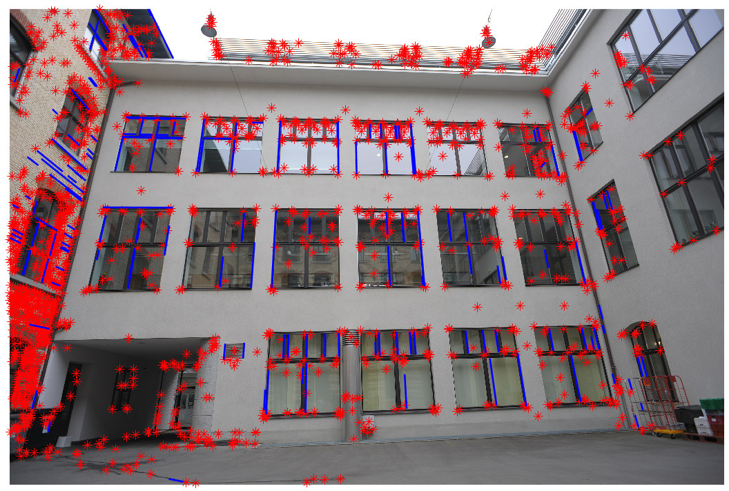
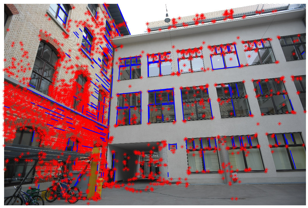
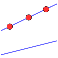
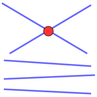
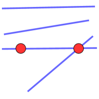
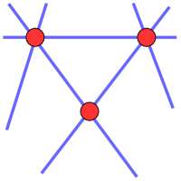
Figure 1: (1-st row) Points (red) and lines (blue) get detected independently as well as in arrangements with points incident to lines [36]. (2-nd row) Examples of some interesting arrangements of points and lines providing new minimal problems. See Tab. 1 for the complete classification of minimal problems for points, lines and their arrangements in multiple images with complete multi-view visibility.

Contribution  We give a complete classification of minimal problems for generic arrangements of points and lines, including their incidences, completely observed by any number of calibrated perspective cameras. We consider calibrated scenarios since it avoids many degeneracies [15].

We show that there are exactly $30$ minimal point-line problems (up to an arbitrary number of lines in the case of two views) when considering complete visibility (Tab. 1). In particular, there is no such minimal problem for seven or more cameras. For $6$, $5$, $4$ and $3$ cameras, there are $1$, $3$, $6$ and $17$ minimal problems, respectively. For two views, there are three combinatorial constellations of five points which yield minimal problems. We observe that each minimal point-line problem has at most five points and at most six lines (except for arbitrarily many lines in the case of two views.) Problems $5000_{2}$ [37], $3200_{3}$ [13, 34], $3010_{0},1040_{0}$ [21] have been known before, all other 26 minimal problems in Tab. 1, as far as we know, are new.

For each minimal problem, we compute its algebraic degree which is its number of solutions over the complex numbers for generic images. This degree measures the intrinsic difficulty of a minimal problem. We observe how this degree generally grows with the number of cameras, but we also found several minimal problems with small degrees (32, 40 and 64), which might be practical in image matching and 3D reconstruction [47].

We consider generic minimal problems, i.e. the problems that have a finite number of complex solutions and are generic in the sense that random noise in image measurements does not change the number of solutions. For instance, the classical problem of five points in two views [37] is minimal and one can add arbitrarily many lines to the arrangement in $3$-space; as long as it contains five points in sufficiently generic position, it is still minimal. On the other hand, the problem of four points in three views [31, 18, 40, 42] is overconstrained when all measurements and equations are used. It becomes inconsistent for noisy image measurements. Thus it is not a minimal problem for us.

We assume complete visibility, i.e. all points and lines are observed in all images and all observed information is used to formulate minimal problems. Complete point-line incidence correspondences arise when, e.g. , SIFT point features [32] are considered together with their orientation, lines are constructed from matched affine frames [35], or obtained as simultaneous point and line detections [36], Fig. 1. On the other hand, we do not cover cases that require partial visibility, e.g. , 3 PPP + 1 PPL in [21]. Full account for partial visibility is a much harder task and will be addressed in the future.

We explicitly model point-line incidences. Several lines may be incident to a single point (n-quiver) and several points may be dependent by lying on a single line. We assume that such relations are not broken by image noise since they are constructed by the feature detection process.

Our problem formulation uses direct geometrical determinantal constraints as in [19, 41], not multi-view tensors, since it works for any number of cameras and can model point-line incidences. On the other hand, our formulation is not the most economical for the minimal problem with five independent points in two views ($5000_{2}$ in Tab. 1). This problem has degree $20$ in our formulation while the degree is only 10 when reformulated [38] as a problem of finding the essential matrix.

Structure of the paper

The paper is organized as follows. We review previous work in Sec. 2. Section 3 defining main concepts is followed by problem specification in Sec. 4. All candidates for minimal problems satisfying balanced counts of degrees of freedom are identified in Sec. 5. Section 6 presents our parameterization of the problems for computational purposes. Procedures for checking the minimality and computing the degrees using symbolic and numerical methods from algebraic geometry are presented in Sec. 7.

2 Previous work

Here we review the most relevant work for point-line incidences and minimal problems. See [30, 25, 21] for references on minimal problems in general. Using correspondences of non-incident points and lines in three uncalibrated views was considered in works on the trifocal tensor [16]. The early work on point-line incidences [19] introduced n-quivers, i.e. points incident with n lines in uncalibrated views, and studied minimal problems arising from three 1-quivers in three affine views and three 3-quivers in three perspective views, as well as the overconstrained problem of four 2-quivers in three views.

Uncalibrated multi-view constraints for points, lines and their incidences appeared in [33]. In [41], non-incident points and lines in uncalibrated views were studied and four points and three lines in three views, two points and six lines in three views, and nine lines in three views cases were presented. The solver for the latter case has recently appeared in [27]. Absolute pose of cameras with unknown focal length from 2D-3D quiver correspondences has been solved in [23] for two points and 1-quiver, for one 1-quiver and one 2-quiver, and for four lines. In [11], an important case, when lines incident to points arise from tangent lines to curves, is presented. It motivates the case with three points and tangent lines at two points (case $3002_{1}$ in Tab. 1). Work [36] presents several minimal problems for generalized camera absolute pose computation from 2D-3D correspondences of non-incident points and lines with focus on cases when a closed-form solution could be found. In [10, 45], parallelism and perpendicularity of lines in space were exploited to find calibrated relative pose from lines and points. Recent work [55] investigates calibrated relative camera pose problems from two views with 2-quivers with known angles between the 3D lines generating the quivers. Minimal problems for finding the relative pose from three such correspondences for the generic as well as several more specific cases is derived. Our closest generalization of this result is that one can obtain calibrated relative pose of three cameras from one 2-quiver and two independent points in three views without knowing angles in 3D. Recently, minimal problems were constructed for local multi-features including lines incident to points as well as more complex features [7, 5, 6]. They build on SIFT directions [32] or more elaborate local affine features [35] to reduce the number of samples needed in RANSAC [43] to verify tentative matches.

The most relevant previous work  Recent theoretical results [20, 1, 2, 3, 53, 54] made steps towards characterizing some of the classes of minimal problems. The most relevant work [21] provided a classification for three calibrated views that can be formulated using linear constraints on the trifocal tensor [15]. In [21], 66 minimal problems for three calibrated views were presented and their algebraic degrees computed. The lowest degree 160 has been observed for one PPP and four PPL constraints while the highest degree 4912 has been observed for 11 PLL constraints. Out of 66 problems in [21] the ones that can be modeled with complete visibility are (1 PPP + 4 LLL) and (3 PPP + 1 LLL). These two minimal problems appear as $1040_{0}$ and $3010_{0}$ in Tab. 1. The other 15 minimal problems in three views that we discovered do not appear in [21] since the point-line incidences were not considered.

3 Notation and concepts

We use nomenclature from [15]. Points and lines in space are in the projective space $\mathbb{P}^{3}$, image points are in $\mathbb{P}^{2}$ and are represented by homogeneous coordinates. We consider the Grassmannians $\mathbb{G}_{1,3}$ and $\mathbb{G}_{1,2}$ which are the spaces of lines in $\mathbb{P}^{3}$ and $\mathbb{P}^{2},$ respectively. $\operatorname{\rm SO}(3)$ stands for the special orthogonal group, i.e. rotations, defined algebraicly as $3\times 3$ matrices $R$ such that $RR^{\top}=I$, $\det{R}=1$. All is considered over an arbitrary field $\mathbb{F}$ unless explicitly specified. Coefficients of equations originate from the field $\mathbb{Q}$ of rational numbers. Solutions of the equations are in the field $\mathbb{C}$ of complex numbers. We carry out symbolic computations in a finite field $\mathbb{Z}_{p}$ for a prime $p$ for the sake of exactness and computational efficiency. Numerical algorithms use floating point to approximate complex numbers.

4 Problem Specification

Our main result applies to problems in which points, lines, and point-line incidences are observed. We first introduce a point-line problem as a tuple $({p,l,\mathcal{I},m})$ specifying that $p$ points and $l$ lines in space, which are incident according to a given incidence relation $\mathcal{I}\subset\{1,\ldots,p\}\times\{1,\ldots,l\}$ (i.e. $(i,j)\in\mathcal{I}$ means that the $i$-th point is on the $j$-th line) are projected to $m$ views. So a point-line problem captures the numbers of points, lines and views as well as the incidences between points and lines. We will model intersecting lines by requiring that each intersection point of two lines has to be one of the $p$ points in the point-line problem. Throughout this article we will only consider incidence relations which can be realized by a point-line arrangement in $\mathbb{P}^{3}$. In particular, two distinct lines cannot be incident to the same two distinct points. In addition, we will always assume that the incidence relation $\mathcal{I}$ is complete in the sense that every incidence which is automatically implied by the incidences in $\mathcal{I}$ must also be contained in $\mathcal{I}$. An instance of a point-line problem is specified by the following data:

(1) A point-line arrangement in space consisting of $p$ points $X_{1},\ldots,X_{p}$ and $l$ lines $L_{1},\ldots,L_{l}$ in $\mathbb{P}^{3}$ which are incident exactly as specified by $\mathcal{I}\subset\{1,\ldots,p\}\times\{1,\ldots,l\}$. Hence, the point $X_{i}$ is on the line $L_{j}$ if and only if $(i,j)\in\mathcal{I}$. We write

$$\mathcal{X}_{p,l,\mathcal{I}}=\left\{(X,L)\in\left(\mathbb{P}^{3}\right)^{p}\times\left(\mathbb{G}_{1,3}\right)^{l}\mid\forall(i,j)\in\mathcal{I}\,\colon X_{i}\in L_{j}\right\}$$

for the associated variety of point-line arrangements. Note that this variety also contains degenerate arrangements, where not all points and lines have to be pairwise distinct or where there are more incidences between points and lines than those specified by $\mathcal{I}$.

(2) A list of $m$ calibrated cameras which are represented by matrices

$$P_{1}=[R_{1}\mid t_{1}],\ldots,P_{m}=[R_{m}\mid t_{m}]$$

with $R_{1},\ldots,R_{m}\in\operatorname{\rm SO}(3)$ and $t_{1},\ldots,t_{m}\in\mathbb{F}^{3}$.

(3) The joint image consisting of the projections $x_{v,1},\ldots,x_{v,p}\in\mathbb{P}^{2}$ of the points $X_{1},\ldots,X_{p}$ and the projections $\ell_{v,1},\ldots,\ell_{v,l}\in\mathbb{G}_{1,2}$ of the lines $L_{1},\ldots,L_{l}$ by the cameras $P_{1},\ldots,P_{m}$ to the $v=1,\ldots,m$ views. We write

$$\mathcal{Y}_{p,l,\mathcal{I},m}=\left\{(x,\ell)\in\left(\mathbb{P}^{2}\right)^{m\,p}\times\left(\mathbb{G}_{1,2}\right)^{m\,l}\;\middle|\;\forall v=1,\ldots,m\;\forall(i,j)\in\mathcal{I}:x_{v,i}\in\ell_{v,j}\right\}$$

for the image variety which consists of all $m$-tuples of two-dimensional point-line arrangements which satisfy the incidences specified by $\mathcal{I}$.

Given a joint image, we want to recover an arrangement in space and cameras yielding the given joint image. We refer to a pair of such an arrangement and such a list of $m$ cameras as a solution of the point-line problem for the given joint image. We note that an $m$-tuple in $\mathcal{Y}_{p,l,\mathcal{I},m}$ does not necessarily admit a solution, i.e. a priori it does not have to be a joint image of a common point-line arrangement in $3$-space.

To fix the arbitrary space coordinate system [15], we set $P_{1}=[I\,|\,0]$ and the first coordinate of $t_{2}$ to $1$. Hence, our camera configurations are parameterized by

$$\mathcal{C}_{m}=\left\{(P_{1},\ldots,P_{m})\in\left(\mathbb{F}^{3\times 4}\right)^{m}\;\middle|\;P_{i}=[R_{i}\mid t_{i}],\,R_{i}\in\operatorname{\rm SO}(3),t_{i}\in\mathbb{F}^{3},\,R_{1}=I,t_{1}=0,t_{2,1}=1\right\}.$$

We will always assume that the camera positions in an instance of a point-line problem are sufficiently generic such that the following three natural conditions are satisfied for each camera: Firstly, two distinct lines or points in the given arrangement in $3$-space are viewed as distinct lines or points. Secondly, a point and a line in the space arrangement, which are not incident in $3$-space, are viewed as non-incident. Thirdly, three non-colinear points in the space arrangement are viewed as non-colinear points.

We say that a point-line problem is minimal if a generic image tuple in $\mathcal{Y}_{p,l,\mathcal{I},m}$ has a nonzero finite number of solutions. We may phrase this definition formally:

Definition 1.

Let $\Phi_{p,l,\mathcal{I},m}:\mathcal{X}_{p,l,\mathcal{I}}\times\mathcal{C}_{m}\dashrightarrow\mathcal{Y}_{p,l,\mathcal{I},m}$ denote the joint camera map, which sends a point-line arrangement in space and $m$ cameras to the resulting joint image. We say that the point-line problem $({p,l,\mathcal{I},m})$ is minimal if

• $\Phi_{p,l,\mathcal{I},m}$ is a dominant map, i.e.  a generic element $(x,\ell)$ in $\mathcal{Y}_{p,l,\mathcal{I},m}$ has a solution, so $\Phi_{p,l,\mathcal{I},m}^{-1}(x,\ell)\neq\emptyset$, and

• the preimage $\Phi_{p,l,\mathcal{I},m}^{-1}(x,\ell)$ of a generic element $(x,\ell)$ in $\mathcal{Y}_{p,l,\mathcal{I},m}$ is finite.

Remark 1.

For a given a minimal problem $({p,l,\mathcal{I},m}),$ the joint camera map $\Phi_{p,l,\mathcal{I},m}$ maps $\mathcal{X}_{p,l,\mathcal{I}}\times\mathcal{C}_{m}$ onto a constructible subset of $\mathcal{Y}_{p,l,\mathcal{I},m}$ of the same dimension. Given a solution for a generic joint image $(x,\ell)$ when $\mathbb{F}=\mathbb{R}$ or $\mathbb{C},$ there exists a ball around $(x,\ell),$ say $B_{\epsilon}(x,\ell),$ and for each solution $(X,C)\in\Phi_{p,l,\mathcal{I},m}^{-1}(x,\ell)$ a ball $B_{\delta}(X,C)$ such that

$$\Phi_{p,l,\mathcal{I},m}\left(B_{\delta}(X,C)\right)\subset B_{\epsilon}(x,\ell).$$

In this sense, we may deduce that solutions to minimal problems are stable under perturbation of the data.

The joint camera map $\Phi_{p,l,\mathcal{I},m}$ reflects that we want to recover world points and lines as well as camera poses from a given joint image. In the case of complete visibility, this is equivalent to only recovering camera poses. We formalize this observation in Lemma 2 and Corollary 2.

Over the complex numbers, the cardinality of the preimage $\Phi_{p,l,\mathcal{I},m}^{-1}(x,\ell)$ is the same for every generic joint image $(x,\ell)$ of a minimal point-line problem $({p,l,\mathcal{I},m})$. We refer to this cardinality as the degree of the minimal problem. Our goal is to list all minimal point-line problems and to compute their degrees. For this, we pursue the following strategy:

Step 1: A classical statement from algebraic geometry states for a dominant map $\varphi:X\dashrightarrow Y$ from a variety $X$ to another variety $Y$ that the preimage $\varphi^{-1}(y)$ of a generic point $y$ in $Y$ has dimension $\dim(X)-\dim(Y).$ When $\varphi$ is a linear map between linear spaces, this is simply the rank-nullity theorem of linear algebra. As the generic preimage of the joint camera map $\Phi_{p,l,\mathcal{I},m}$ associated to a minimal point-line problem $({p,l,\mathcal{I},m})$ is zero-dimensional, we see that every minimal point-line problem must satisfy the equality $\dim(\mathcal{X}_{p,l,\mathcal{I}}\times\mathcal{C}_{m})=\dim(\mathcal{Y}_{p,l,\mathcal{I},m})$. This motivates the following definition.

Definition 2.

We say that a point-line problem $({p,l,\mathcal{I},m})$ is balanced if $\dim(\mathcal{X}_{p,l,\mathcal{I}}\times\mathcal{C}_{m})=\dim(\mathcal{Y}_{p,l,\mathcal{I},m})$.

As we have now established that all minimal point-line problems are balanced, we classify all balanced point-line problems in Sec. 5. We will see that there are only finitely many such problems, explicitly given in Tab. 1, up to arbitrarily many lines in the case of two views; see Remark 2.

Step 2: The classical statement from algebraic geometry mentioned above further implies that a balanced point-line problem $({p,l,\mathcal{I},m})$ is minimal if and only if its joint camera map $\Phi_{p,l,\mathcal{I},m}$ is dominant. Hence, to determine the exhaustive list of all minimal point-line problems, we only have to check for each balanced point-line problem in Tab. 1 if its joint camera map is dominant. We perform this check computationally, as described in Sec. 7.

Step 3: Finally, we use symbolic and numerical computations to calculate the degrees of the minimal point-line problems. We describe these computations in Sec. 7.

Table 1: All balanced point-line problems, modulo adding arbitrarily many lines to the problems with $2$ views. Some problems are not uniquely identified by their vector $(p^{\mathrm{f}},p^{\mathrm{d}},l^{\mathrm{f}},l^{\mathrm{a}})$. To make the identification unique, we extend the vector by a subscript $\alpha$, which is the maximum number of lines adjacent to the same point in the case of at least three views or the maximum number of points on a common line in the case of two views. Degrees marked with ^∗ have been computed with numerical methods, the others with symbolic algorithms; see Section 7. Problem $3200_{3}$ has all five points in a single 3D plane: it corresponds to the calibrated homography relative pose computation [13, 34]; see Supplementary Material.

$m$ views

6

6

6

5

5

5

4

4

4

4

4

4

4

$p^{\mathrm{f}}p^{\mathrm{d}}l^{\mathrm{f}}l^{\mathrm{a}}_{\alpha}$

$1021_{1}$

$1013_{3}$

$1005_{5}$

$2011_{1}$

$2003_{2}$

$2003_{3}$

$1030_{0}$

$1022_{2}$

$1014_{4}$

$1006_{6}$

$3001_{1}$

$2110_{0}$

$2102_{1}$

$(p,l,\mathcal{I})$

Minimal

Y

N

N

Y

Y

Y

Y

Y

N

N

Y

Y

Y

Degree

$>180k^{*}$

$11296^{*}$

$26240^{*}$

$11008^{*}$

$3040^{*}$

$4512^{*}$

$1728^{*}$

$32^{*}$

$544^{*}$

$m$ views

4

3

3

3

3

3

3

3

3

3

3

3

3

$p^{\mathrm{f}}p^{\mathrm{d}}l^{\mathrm{f}}l^{\mathrm{a}}_{\alpha}$

$2102_{2}$

$1040_{0}$

$1032_{2}$

$1024_{4}$

$1016_{6}$

$1008_{8}$

$2021_{1}$

$2013_{2}$

$2013_{3}$

$2005_{3}$

$2005_{4}$

$2005_{5}$

$3010_{0}$

$(p,l,\mathcal{I})$

Minimal

Y

Y

Y

Y

N

N

Y

Y

Y

Y

Y

Y

Y

Degree

$544^{*}$

360

552

480

264

432

328

480

240

64

216

$m$ views

3

3

3

3

3

3

3

3

2

2

2

2

2

$p^{\mathrm{f}}p^{\mathrm{d}}l^{\mathrm{f}}l^{\mathrm{a}}_{\alpha}$

$3002_{1}$

$3002_{2}$

$2111_{1}$

$2103_{1}$

$2103_{2}$

$2103_{3}$

$3100_{0}$

$2201_{1}$

$5000_{2}$

$4100_{3}$

$3200_{3}$

$3200_{4}$

$2300_{5}$

$(p,l,\mathcal{I})$

Minimal

Y

Y

Y

Y

Y

Y

Y

N

Y

Y

Y

N

N

Degree

312

224

40

144

144

144

64

20

16

12

5 Balanced Point-Line Problems

To understand balanced point-line problems we need to derive formulas for the dimensions of the varieties $\mathcal{X}_{p,l,\mathcal{I}}$, $\mathcal{C}_{m}$ and $\mathcal{Y}_{p,l,\mathcal{I},m}$. As $\operatorname{\rm SO}(3)$ is three-dimensional, and we set the first camera to $[I|0]$ and one parameter in the second camera to $1$, the parameter space of camera configurations for $m\geq 2$ has dimension $\dim(\mathcal{C}_{m})=6m-7.$

Let us now consider a generic point-line arrangement in $\mathcal{X}_{p,l,\mathcal{I}}$. Some of its points may be dependent on other points, in the sense that such a dependent point lies on a line spanned by two other points. In any arrangement of points in $3$-space, each minimal set of independent points has the same cardinality. For our arrangement of $p$ points we denote this cardinality by $p^{\mathrm{f}}$ (the upper index $\mathrm{f}$ stands for free). We write $p^{\mathrm{d}}=p-p^{\mathrm{f}}$ for the number of dependent points. Each free point is defined by three parameters. A dependent point $X$ is only defined by one further parameter after the two points, which span the line containing $X$, are defined. In total, the $p$ points in our arrangement are defined by $3\,p^{\mathrm{f}}+p^{\mathrm{d}}$ parameters. Each of the $l$ lines in our arrangement is either incident to zero, one or at least two points. We refer to lines which are incident to no points as free lines. We denote the number of free lines by $l^{\mathrm{f}}$. As the Grassmannian $\mathbb{G}_{1,3}$ of lines is four-dimensional, each free line is defined by four parameters. A line which is incident to a fixed point is defined by only two parameters. We denote the number of lines which are incident to exactly one point by $l^{\mathrm{a}}$ (the upper index $\mathrm{a}$ stands for adjacent). Finally, each of the remaining $l-l^{\mathrm{f}}-l^{\mathrm{a}}$ lines is incident to at least two points and thus already uniquely determined by the two points. Hence, we have derived

$$\dim(\mathcal{X}_{p,l,\mathcal{I}})=3\,p^{\mathrm{f}}+p^{\mathrm{d}}+4\,l^{\mathrm{f}}+2\,l^{\mathrm{a}}.$$ (1)

In particular, we see that we might as well assume that there is no line passing through two or more points, as such lines do not contribute to our parameter count.

We derive the dimension of the image variety $\mathcal{Y}_{p,l,\mathcal{I},m}$ similarly. Since we assume all camera positions to be sufficiently generic, each camera views exactly $p^{\mathrm{f}}$ independent points, $p^{\mathrm{d}}$ dependent points, $l^{\mathrm{f}}$ free lines and $l^{\mathrm{a}}$ lines which are incident to exactly one of the points. Each independent point is defined by two parameters, whereas each dependent point is defined by a single parameter. A free line is defined by two parameters. A line which is incident to a fixed point is defined by a single parameter. All in all, we have that

$$\dim(\mathcal{Y}_{p,l,\mathcal{I},m})=m\,(2\,p^{\mathrm{f}}+p^{\mathrm{d}}+2\,l^{\mathrm{f}}+l^{\mathrm{a}}).$$ (2)

Note that there is no balanced point-line problem for a single camera. For $m>1$ cameras, combining $\dim(\mathcal{C}_{m})=6m-7$ with  (1) and (2) yields that a point-line problem is balanced if and only if

$$3\,p^{\mathrm{f}}+p^{\mathrm{d}}+4\,l^{\mathrm{f}}+2\,l^{\mathrm{a}}+6\,m-7=m\left(2\,p^{\mathrm{f}}+p^{\mathrm{d}}+2\,l^{\mathrm{f}}+l^{\mathrm{a}}\right).$$

This is equivalent to

$$6m\!-\!7\!=\!(2m\!-\!3)p^{\mathrm{f}}\!+\!(m\!-\!1)p^{\mathrm{d}}\!+\!2(m\!-\!2)l^{\mathrm{f}}\!+\!(m\!-\!2)l^{\mathrm{a}}.$$ (3)

Lemma 1.

Every balanced point-line problem with at least five points has exactly two cameras.

Proof.

Suppose $({p,l,\mathcal{I},m})$ is a balanced point-line problem with $m>1$ cameras and at least five points, i.e. $p^{\mathrm{f}}+p^{\mathrm{d}}\geq 5$. In this case, the equality (3) implies

$$6m\!-\!7\geq(2m\!-\!3)p^{\mathrm{f}}\!+\!(m\!-\!1)(5\!-\!p^{\mathrm{f}})\!=\!(p^{\mathrm{f}}\!+\!5)m\!-\!(2p^{\mathrm{f}}\!+\!5),$$

which is equivalent to

$$2(p^{\mathrm{f}}-1)\geq(p^{\mathrm{f}}-1)m.$$ (4)

Among the five or more points at least two have to be (by definition) independent, i.e. $p^{\mathrm{f}}>1$. So (4) yields $m\leq 2$. ∎

Theorem 1.

There is no balanced point-line problem with seven or more cameras.

Proof.

Let $({p,l,\mathcal{I},m})$ be a balanced point-line problem with $m\geq 7$ cameras. By equality (3), we have

$$5\equiv p^{\mathrm{f}}+p^{\mathrm{d}}\mod(m-2).$$ (5)

This implies $p^{\mathrm{f}}+p^{\mathrm{d}}\geq 5$ if $m\geq 8$, which contradicts Lemma 1, and thus we have only one remaining case to check: $m=7$. From (5) and Lemma 1, we have $p^{\mathrm{f}}+p^{\mathrm{d}}=0$ in the case of seven cameras. It means that there are no points, and thus there cannot be lines which are incident to points. So we have $p^{\mathrm{f}}=0$, $p^{\mathrm{d}}=0$, $l^{\mathrm{a}}=0$, and (3) reduces to $35=10l^{\mathrm{f}}$, which is clearly not possible. So there are no balanced point-line problems with seven or more cameras. ∎

Theorem 2.

There are $34$ balanced point-line problems with $3$, $4$, $5$ or $6$ cameras. They are all listed in Tab. 1.

Proof.

We consider the different cases for $3\leq m\leq 6$ and reason by cases.

$\bullet\ m=6$: Due to (5) and Lemma 1, every balanced point-line problem with six cameras must have exactly one point. So we have $p^{\mathrm{f}}=1$, $p^{\mathrm{d}}=0$, and (3) reduces to $5=2l^{\mathrm{f}}+l^{\mathrm{a}}$. This gives us three possibilities: $(l^{\mathrm{f}},l^{\mathrm{a}})\in\{(2,1),(1,3),(0,5)\}$ (see first row of Tab. 1).

$\bullet\ m=5$: Due to (5) and Lemma 1, every balanced point-line problem with five cameras must have exactly two points. So we have $p^{\mathrm{f}}=2$, $p^{\mathrm{d}}=0$, and (3) reduces to $3=2l^{\mathrm{f}}+l^{\mathrm{a}}$. This gives us two possibilities: $(l^{\mathrm{f}},l^{\mathrm{a}})\in\{(1,1),(0,3)\}$, which yield three point-line problems (see the first row of Tab. 1).

$\bullet\ m=4$: Due to (5) and Lemma 1, every balanced point-line problem with four cameras must have either one point or three points. Let us first consider the case of a single point. Here we have $p^{\mathrm{f}}=1$, $p^{\mathrm{d}}=0$, and (3) reduces to $6=2l^{\mathrm{f}}+l^{\mathrm{a}}$. This gives us four possibilities: $(l^{\mathrm{f}},l^{\mathrm{a}})\in\{(3,0),(2,2),(1,4),(0,6)\}$ (see first row of Tab. 1). Secondly, we consider balanced point-line problems with four cameras and three points. If all three points are independent, (3) reduces to $1=2l^{\mathrm{f}}+l^{\mathrm{a}}$, which has a single solution: $(l^{\mathrm{f}},l^{\mathrm{a}})=(0,1)$. If not all three points are independent, we have $p^{\mathrm{f}}=2$, $p^{\mathrm{d}}=1$, and (3) reduces to $2=2l^{\mathrm{f}}+l^{\mathrm{a}}$. This gives us two possibilities: $(l^{\mathrm{f}},l^{\mathrm{a}})\in\{(1,0),(0,2)\}$, which yield three point-line problems (see the first two rows of Tab. 1 for all four point-line problems with four cameras and three points).

$\bullet\ m=3$: We first observe that each balanced point-line problem with three cameras must have at least one point. Otherwise we would have $p^{\mathrm{f}}=0$, $p^{\mathrm{d}}=0$ and $l^{\mathrm{a}}=0$, so (3) would reduce to $11=2l^{\mathrm{f}}$, which is impossible. Let us first consider the case of a single point. Here we have $p^{\mathrm{f}}=1$, $p^{\mathrm{d}}=0$, and (3) reduces to $8=2l^{\mathrm{f}}+l^{\mathrm{a}}$. This gives us five possibilities: $(l^{\mathrm{f}},l^{\mathrm{a}})\in\{(4,0),(3,2),(2,4),(1,6),(0,8)\}$ (see second row of Tab. 1). Secondly, in the case of two points, we have $p^{\mathrm{f}}=2$, $p^{\mathrm{d}}=0$, and (3) reduces to $5=2l^{\mathrm{f}}+l^{\mathrm{a}}$. This gives us three possibilities: $(l^{\mathrm{f}},l^{\mathrm{a}})\in\{(2,1),(1,3),(0,5)\}$, which yield six point-line problems (see second row of Tab. 1). Thirdly, we consider the case of three points. If all three points are independent, (3) reduces to $2=2l^{\mathrm{f}}+l^{\mathrm{a}}$. The two solutions $(l^{\mathrm{f}},l^{\mathrm{a}})\in\{(1,0),(0,2)\}$ yield three point line problems (see last two rows of Tab. 1). If not all three points are independent, we have $p^{\mathrm{f}}=2$, $p^{\mathrm{d}}=1$, and (3) reduces to $3=2l^{\mathrm{f}}+l^{\mathrm{a}}$. The two solutions $(l^{\mathrm{f}},l^{\mathrm{a}})\in\{(1,1),(0,3)\}$ yield four point-line problems (see last row of Tab. 1). Finally, we consider balanced point-line problems with three cameras and four points. We see from (3) that not all four points can be independent. Hence, we either have $p^{\mathrm{f}}=3$ and $p^{\mathrm{d}}=1$ such that (3) reduces to $0=2l^{\mathrm{f}}+l^{\mathrm{a}}$, which has a single solution $(l^{\mathrm{f}},l^{\mathrm{a}})=(0,0)$, or we have $p^{\mathrm{f}}=2$ and $p^{\mathrm{d}}=2$ such that (3) reduces to $1=2l^{\mathrm{f}}+l^{\mathrm{a}}$, which also has a single solution $(l^{\mathrm{f}},l^{\mathrm{a}})=(0,1)$ (see the last row of Tab. 1) ∎

Remark 2.

For the case of two cameras, we see from (3) that the number of free and incident lines do not contribute to the parameter count for balanced point-line problems. In fact, (3) reduces for $m=2$ to $5=p^{\mathrm{f}}+p^{\mathrm{d}}$. Hence, we have the classical minimal problem of recovering five points from two camera images. More precisely, a point-line problem with two cameras is balanced if and only if it has five points. Therefore, it is irrelevant how many lines are contained in the arrangement or how many points are independent. There are $5$ combinatorial possibilities to distribute dependent and independent points (see the last row of Tab. 1).

Corollary 1.

There are 39 balanced point-line problems, modulo any number of lines in the case of two views. They are listed in Tab. 1.

6 Eliminating world points and lines

In order to do computations, it is customary to describe problems with implicit equations that do not depend on the world variables. Before we describe such equations, let us phrase the elimination of the world variables geometrically.

We consider the Zariski closure of the graph of the joint camera map:

$$\mathrm{Inc}=\overline{\{(X,C,Y)\in\mathcal{X}_{p,l,\mathcal{I}}\times\mathcal{C}_{m}\times\mathcal{Y}_{p,l,\mathcal{I},m}\mid}\hskip 28.45274pt$$

$$\overline{Y=\Phi_{p,l,\mathcal{I},m}(X,C)\}}.$$

The joint camera map $\Phi_{p,l,\mathcal{I},m}$ is dominant if and only if the projection $\pi_{\mathcal{Y}}:\mathrm{Inc}\to\mathcal{Y}_{p,l,\mathcal{I},m}$ onto the last factor is dominant (since this is the projection from the graph of $\Phi_{p,l,\mathcal{I},m}$ on its codomain). Moreover, the cardinality of the preimage of a generic point $Y\in\mathcal{Y}_{p,l,\mathcal{I},m}$ under both maps $\Phi_{p,l,\mathcal{I},m}$ and $\pi_{\mathcal{Y}}$ is the same.

To make computations simpler, we want to derive the same statement for the following restricted incidence variety, which does not include the 3D structure $\mathcal{X}_{p,l,\mathcal{I}}$:

$$\mathrm{Inc}^{\prime}=\overline{\{(C,Y)\in\mathcal{C}_{m}\times\mathcal{Y}_{p,l,\mathcal{I},m}\mid}\hskip 56.9055pt$$

$$\overline{\exists X\in\mathcal{X}_{p,l,\mathcal{I}}:Y=\Phi_{p,l,\mathcal{I},m}(X,C)\}}.$$

We have the following canonical projections:

where $\pi_{\mathcal{C},\mathcal{Y}}$ omits the first factor and $\pi^{\prime}_{\mathcal{Y}}$ projects onto the last factor.

Lemma 2.

If $m\geq 2$, a generic point $(C,Y)\in\mathrm{Inc}^{\prime}$ has a single point in its preimage under $\pi_{\mathcal{C},\mathcal{Y}}$.

Proof.

$Y=(x,\ell)$ consists of points $x=(x_{1,1},\ldots,x_{m,p})$ and lines $\ell=(\ell_{1,1},\ldots,\ell_{m,l})$ in the $m$ views. Each point $x_{v,i}\in\mathbb{P}^{2}$ in a view $v$ is pulled back via the $v$-th camera to a line in $3$-space. As $m\geq 2$, the $m$ pull-back lines for generic $x_{1,i},\ldots,x_{m,i}$ intersect in a unique point in $\mathbb{P}^{3}$. Similarly, each line $\ell_{v,j}$ in a view $v$ is pulled back via the $v$-th camera to a plane in $\mathbb{P}^{3}$. As $m\geq 2$, the $m$ generic pull-back planes for $\ell_{1,j},\ldots,\ell_{m,j}$ intersect in a unique line in $\mathbb{P}^{3}$. ∎

Corollary 2.

A balanced point-line problem $({p,l,\mathcal{I},m})$ is minimal if and only if the projection $\pi^{\prime}_{\mathcal{Y}}$ is dominant. In that case, the degree of the minimal problem is the cardinality of the preimage ${\pi^{\prime}_{\mathcal{Y}}}^{-1}(Y)$ of a generic joint image $Y\in\mathcal{Y}_{p,l,\mathcal{I},m}$ over the complex numbers.

Proof.

As we have observed in Step 2 in Section 4, a balanced point-line problem is minimal if and only if its joint camera map $\Phi_{p,l,\mathcal{I},m}$ is dominant. This happens if and only if $\pi_{\mathcal{Y}}$ is dominant. Due to Lemma 2, this is equivalent to that $\pi^{\prime}_{\mathcal{Y}}$ is dominant. Similarly, for a generic $Y\in\mathcal{Y}_{p,l,\mathcal{I},m}$, the cardinalities of the preimages $\Phi_{p,l,\mathcal{I},m}^{-1}(Y)$, $\pi_{\mathcal{Y}}^{-1}(Y)$ and ${\pi^{\prime}_{\mathcal{Y}}}^{-1}(Y)$ coincide due to Lemma 2. ∎

We note that it is possible to describe the variety $\mathrm{Inc}^{\prime}$ as a component of the variety cut out by the equations that we establish in the remainder of this section.

For any instance of a point-line problem, the solutions must satisfy certain equations defined in terms of joint images $(x,\ell)\in\mathcal{Y}_{p,l,\mathcal{I},m}.$ Our scheme for generating such equations relies on an alternate representation of $(x,\ell)$ defined solely in terms of lines. The equations result from two types of constraints. The first type of constraint is a line correspondence (LC): if $\ell_{1},\ldots,\ell_{m}$ are images of the same world line, with respective homogeneous coordinates ${\mathbf{l}}_{1},\ldots,{\mathbf{l}}_{m}\in\mathbb{F}^{3\times 1},$ then

$$\operatorname{rank}\begin{bmatrix}P_{1}^{T}{\mathbf{l}}_{1}&P_{2}^{T}{\mathbf{l}}_{2}&\dots&P_{m}^{T}{\mathbf{l}}_{m}\end{bmatrix}\leq 2.$$ (6)

That is, the planes with homogeneous coordinates $P_{i}^{T}{\mathbf{l}}_{i}$ share a common line in $\mathbb{P}^{3}$. We distinguish two classes of lines in $\mathbb{P}^{2}:$

(1) Visible lines define valid line correspondences. Besides $m\,l$ observed lines in the joint image, for generic $x$ there is a unique visible line between any two observed points. Taken across all views, any pair of points thus provides a line correspondence which must be satisfied.

(2) Two generic visible lines suffice to define a point. We may use an additional set of (non-corresponding) ghost lines to define any points which meet fewer than two visible lines. A generic ghost line contains exactly one observed point — it is simply a device for generating equations.

Thus we obtain common point (CP) constraints: given visible and ghost lines ${\mathbf{l}}_{v,1},\ldots{\mathbf{l}}_{v,k_{i}}$ which meet $x_{v,i}$, the projection of the $i$-th point in the view $v\in 1,\dots,m$, we must have

$$\operatorname{rank}\begin{bmatrix}P_{1}^{T}{\mathbf{l}}_{1,1}&\dots&P_{m}^{T}{\mathbf{l}}_{m,k_{i}}\end{bmatrix}\leq 3,\quad i=1,\ldots,p.$$ (7)

We may encode a point-line problem by specifying some number of visible lines, some number of ghost lines, and which of these lines are incident at each point. We illustrate this encoding with several examples appearing in Figure 3:

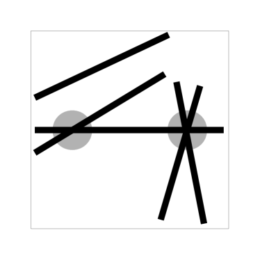
Example (1)

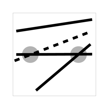
Example (2)

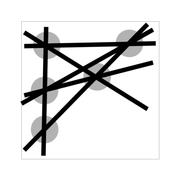
Example (3)

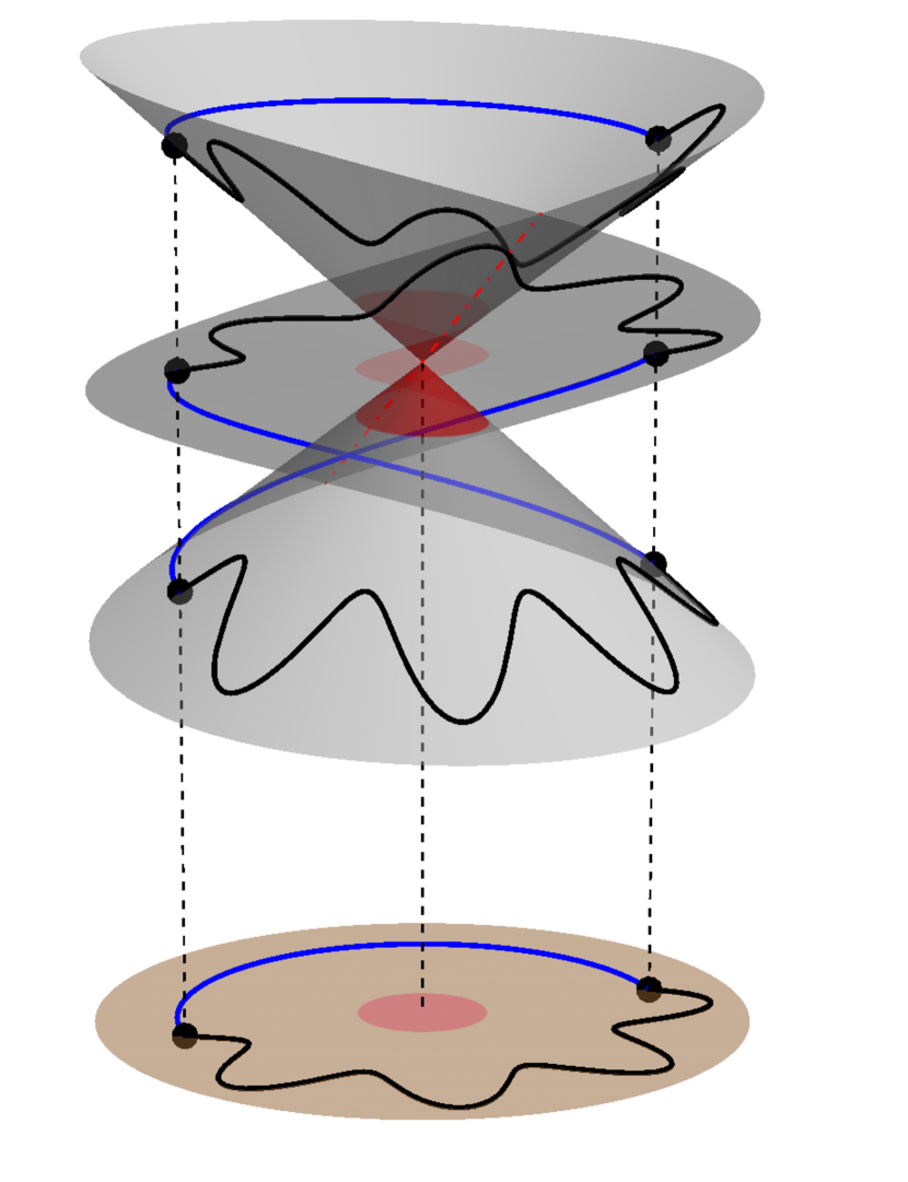
Figure 2: Encoding problems with visible and ghost lines.

Figure 3: Circulating along the path in the parameter space (downstairs) creates a path meeting all solutions (upstairs).

Example 1.

(1) Consider the point-line problem labeled “$2013_{2}$” in Tab. 1. The lines explicitly drawn in the table together with a visible line between the two free points, as in Fig. 3, suffice to define the scene for generic data.

(2) Consider now the problem labeled “$2011_{1}$” in Tab. 1. The encoding given in Fig. 3 includes the given lines, a visible line between the given points, as well as a single ghost line needed to define one of the points.

(3) Finally, consider the problem labeled “$3200_{3}$” in Tab. 1. The extra visible lines appearing in Fig. 3 fix the positions of all points.

LC and CP constraints immediately translate into determinantal conditions: the $3\times 3$ minors of the matrix in (6) must vanish for each visible line, and the $4\times 4$ minors of the matrix in (7) must vanish for each point. Thus, we obtain explicit polynomials for each point-line problem once we fix some encoding and the cameras parametrization, i.e. a rational map $G:\mathbb{F}^{6m-7}\dashedrightarrow\mathcal{C}_{m}$. In our computations, we define $G$ via the Cayley parametrization for $\operatorname{\rm SO}(3)$:

$$R([a,b,c])=(I+\left[[a,b,c]\right]_{\times})(I-\left[[a,b,c]\right]_{\times})^{-1}.$$ (8)

7 Checking minimality & computing degrees

Denote by $F=F_{{p,l,\mathcal{I},m}}$ the system of polynomials resulting from a given point-line problem $({p,l,\mathcal{I},m})$ using our construction of the LC and CP constraints in Sec. 6 with the cameras parameterization $G$ plugged in. The variety of points satisfying $F(C,Y)=0$ contains $\mathrm{Inc}^{\prime}$ as an irreducible component.

Remark 3.

The variety of points satisfying $F(C,Y)=0$ may also have spurious components corresponding to solutions $(C,Y)$ where the ranks of the matrices (6) or (7) are smaller than desired. Such spurious solutions do not correspond to world lines in $\mathbb{G}_{1,3}$ and must be ruled out. These spurious components are naturally avoided by sampling a point on $\mathrm{Inc}^{\prime}$. For implicit symbolic calculations, the spurious solutions may be eliminated by including inequations enforcing nonvanishing of the minors of size one smaller.

The following algorithm checks minimality of a point-line problem locally; geometrically this amounts to passing to the tangent space of $\mathrm{Inc}^{\prime}$.

Algorithm 1 (Minimal).

0:  $({p,l,\mathcal{I},m})$, a balanced point-line problem.

0:  “Y” if the problem is minimal; “N” otherwise.

1:  $J(C,Y)\leftarrow\frac{\partial F(C,Y))}{\partial C}$

2:  Take random $C_{0}\in\mathcal{C}_{m}$ and random $X_{0}\in\mathcal{X}_{p,l,\mathcal{I}}$.

3:  $Y_{0}\leftarrow\Phi_{p,l,\mathcal{I},m}(X_{0},C_{0})$

4:  return  “Y” if $\,\operatorname{rank}J(C_{0},Y_{0})=6m-7,$ else “N.”

Proof of Correctness for Algorithm 1.

In terminology described in the beginning of Sec. 6, the algorithm checks if the conditions of the Inverse Function Theorem hold at a generic point on $\mathrm{Inc}^{\prime}$. If they do, the map $\pi^{\prime}_{\mathcal{Y}}$ is dominant, since in a neighborhood of $Y_{0}$ the map has an inverse: i.e if $Y$ is near $Y_{0}$ then there is $C$ near $C_{0}$ satisfying $F(C,Y)=0$. If these conditions do not hold generically, $\pi^{\prime}_{\mathcal{Y}}$ is not dominant. By Cor. 2, the given point-line problem is minimal if and only if $\pi^{\prime}_{\mathcal{Y}}$ is dominant. ∎

For the minimal problems with two and three views we use the following symbolic algorithm to compute their degrees, i.e. the cardinality of the preimage of a generic joint image $Y\in\mathcal{Y}_{p,l,\mathcal{I},m}$ under the projection $\pi^{\prime}_{\mathcal{Y}}$ (by Cor. 2).

Algorithm 2 (Degree).

0:  $({p,l,\mathcal{I},m})$, a point-line minimal problem.

0:  The degree of this problem.

1:  Take a random $Y_{0}\in\mathcal{Y}_{p,l,\mathcal{I},m}$.

2:  Compute the Gröbner basis $B$ of the ideal generated by $F(C,Y_{0})\subset\mathbb{F}[C]$.

3:  return  the number of monomials in variables $C$ not divisible by the leading monomials of $B$.

Proof of Correctness.

Using Gröbner bases to solve a system of polynomial equations is a standard technique in computational nonlinear algebra. Since we are interested only in the solution count, not the solutions, we are able to carry out computations relatively quickly; see Remark 4. ∎

Remark 4.

Algorithms 1 and 2 are valid over an arbitrary field $\mathbb{F}$. Our main problem is stated over $\mathbb{Q}$, the rational numbers, but since the algorithms rely heavily on symbolic techniques such as Gröbner bases we use the so-called modular technique: we perform computations over a finite field, namely $\mathbb{F}=\mathbb{Z}_{p}$ for $p<2^{15}$. There is a slight chance that this approach fails for a particular exceptional “unlucky” prime $p$, but it is possible to compute the result using several primes and confirm it over $\mathbb{Q}$ via rational reconstruction.

Algorithms 1 and 2 were implemented and executed in the Macaulay2 [14] computer algebra system . Due to limitations of Gröbner basis  algorithms we were unable to compute the degrees of any of the problems with $m>3$ with our implementation of Algorithm 2. On the other hand, the degrees of all minimal problems in Tab. 1 are within reach for the monodromy method, a technique based on numerical homotopy continuation. Specifically, we follow the monodromy solver framework outlined in [9] carrying out computation via a Macaulay2 package MonodromySolver${}^{\text{\ref{M2footnote}}}$. Similar techniques have been successfully employed in a number of studies in applied algebraic geometry [17, 22, 8].

Imagine the projection $\pi^{\prime}_{\mathcal{Y}}:\mathrm{Inc}^{\prime}\dashedrightarrow\mathcal{Y}_{p,l,\mathcal{I},m}$ as the cover map from top to the bottom in Fig. 3. The seed solution $(C_{0},Y_{0})$ produced as in Algorithm 1 is one of the solutions that project to $Y_{0}$ at the bottom. Since the Galois group of $\pi^{\prime}_{\mathcal{Y}}$ acts transitively on the solutions, one can create enough random paths connecting $Y_{0}$ and an auxiliary point $Y_{1}$ so that walking on the liftings of the bottom paths, it is possible to visit all solutions that are above $Y_{0}$ and, hence, discover the degree. See https://github.com/timduff35/PLMPfor code that numerically computes this degree.

8 Conclusion

We characterized a new class of minimal problems and discovered problems with small numbers of solutions that call for constructing their efficient solvers [12].

Acknowledgements

We are grateful to ICERM (NSF DMS-1439786 and the Simons Foundation grant 507536) for the hospitality from September 2018 to February 2019, where most ideas for this project were developed. We also thank the many research visitors at ICERM who participated in fruitful discussions on minimal problems. Research of T. Duff and A. Leykin is supported in part by NSF DMS-1719968. T. Pajdla was supported by the European Regional Development Fund under the project IMPACT (reg. no. CZ.02.1.01/0.0/0.0/15 003/0000468).

References

- [1] Sameer Agarwal, Hon-leung Lee, Bernd Sturmfels, and Rekha R. Thomas. On the existence of epipolar matrices. International Journal of Computer Vision, 121(3):403–415, 2017.
- [2] Chris Aholt and Luke Oeding. The ideal of the trifocal variety. Math. Comput., 83(289):2553–2574, 2014.
- [3] Chris Aholt, Bernd Sturmfels, and Rekha R. Thomas. A hilbert scheme in computer vision. CoRR, abs/1107.2875, 2011.
- [4] Hatem Said Alismail, Brett Browning, and M. Bernardine Dias. Evaluating pose estimation methods for stereo visual odometry on robots. In the 11th International Conference on Intelligent Autonomous Systems (IAS-11), January 2011.
- [5] Daniel Barath. Five-point fundamental matrix estimation for uncalibrated cameras. In 2018 IEEE Conference on Computer Vision and Pattern Recognition, CVPR 2018, Salt Lake City, UT, USA, June 18-22, 2018, pages 235–243, 2018.
- [6] Daniel Barath and Levente Hajder. Efficient recovery of essential matrix from two affine correspondences. IEEE Trans. Image Processing, 27(11):5328–5337, 2018.
- [7] Daniel Barath, Tekla Toth, and Levente Hajder. A minimal solution for two-view focal-length estimation using two affine correspondences. In 2017 IEEE Conference on Computer Vision and Pattern Recognition, CVPR 2017, Honolulu, HI, USA, July 21-26, 2017, pages 2557–2565, 2017.
- [8] Paul Breiding, Bernd Sturmfels, and Sascha Timme. 3264 conics in a second. arXiv preprint arXiv:1902.05518, 2019.
- [9] Timothy Duff, Cvetelina Hill, Anders Jensen, Kisun Lee, Anton Leykin, and Jeff Sommars. Solving polynomial systems via homotopy continuation and monodromy. IMA Journal of Numerical Analysis, 2018.
- [10] Ali Elqursh and Ahmed M. Elgammal. Line-based relative pose estimation. In CVPR 2011.
- [11] Ricardo Fabbri and Benjamin B. Kimia. Multiview differential geometry of curves. International Journal of Computer Vision, 120(3):324–346, 2016.
- [12] R. Fabri et al. Trifocal relative pose from lines at points and its efficient solution. Preprint arXiv:1903.09755, 2019.
- [13] Olivier D. Faugeras and Francis Lustman. Motion and structure from motion in a piecewise planar environment. International Journal of Pattern Recognition and Artificial Intelligence, 2(3):485–508, 1988.
- [14] Daniel R. Grayson and Michael E. Stillman. Macaulay2, a software system for research in algebraic geometry. Available at http://www.math.uiuc.edu/Macaulay2/.
- [15] Richard Hartley and Andrew Zisserman. Multiple View Geometry in Computer Vision. Cambridge, 2nd edition, 2003.
- [16] Richard I. Hartley. Lines and points in three views and the trifocal tensor. International Journal of Computer Vision, 22(2):125–140, 1997.
- [17] Jonathan D. Hauenstein, Luke Oeding, Giorgio Ottaviani, and Andrew J. Sommese. Homotopy techniques for tensor decomposition and perfect identifiability. Journal für die reine und angewandte Mathematik (Crelles Journal), 2016.
- [18] Robert J. Holt and Arun N. Netravali. Uniqueness of solutions to three perspective views of four points. IEEE Trans. Pattern Anal. Mach. Intell., 17(3):303–307, 1995.
- [19] Björn Johansson, Magnus Oskarsson, and Kalle Åström. Structure and motion estimation from complex features in three views. In ICVGIP 2002, Proceedings of the Third Indian Conference on Computer Vision, Graphics & Image Processing, Ahmadabad, India, December 16-18, 2002, 2002.
- [20] Michael Joswig, Joe Kileel, Bernd Sturmfels, and André Wagner. Rigid multiview varieties. IJAC, 26(4):775–788, 2016.
- [21] Joe Kileel. Minimal problems for the calibrated trifocal variety. CoRR, abs/1611.05947, 2016.
- [22] Kathlén Kohn, Boris Shapiro, and Bernd Sturmfels. Moment varieties of measures on polytopes. arXiv preprint arXiv:1807.10258, 2018.
- [23] Yubin Kuang and Kalle Åström. Pose estimation with unknown focal length using points, directions and lines. In IEEE International Conference on Computer Vision, ICCV 2013, Sydney, Australia, December 1-8, 2013, pages 529–536, 2013.
- [24] Zuzana Kukelova, Martin Bujnak, and Tomas Pajdla. Automatic generator of minimal problem solvers. In European Conference on Computer Vision (ECCV), 2008.
- [25] Zuzana Kukelova, Joe Kileel, Bernd Sturmfels, and Tomas Pajdla. A clever elimination strategy for efficient minimal solvers. In Computer Vision and Pattern Recognition (CVPR). IEEE, 2017.
- [26] Viktor Larsson, Kalle Åström, and Magnus Oskarsson. Efficient solvers for minimal problems by syzygy-based reduction. In Computer Vision and Pattern Recognition (CVPR), 2017.
- [27] Viktor Larsson, Kalle Åström, and Magnus Oskarsson. Efficient solvers for minimal problems by syzygy-based reduction. In 2017 IEEE Conference on Computer Vision and Pattern Recognition, CVPR 2017, Honolulu, HI, USA, July 21-26, 2017, pages 2383–2392, 2017.
- [28] Viktor Larsson, Kalle Åström, and Magnus Oskarsson. Polynomial solvers for saturated ideals. In IEEE International Conference on Computer Vision, ICCV 2017, Venice, Italy, October 22-29, 2017, pages 2307–2316, 2017.
- [29] Viktor Larsson, Zuzana Kukelova, and Yinqiang Zheng. Making minimal solvers for absolute pose estimation compact and robust. In International Conference on Computer Vision (ICCV), 2017.
- [30] Viktor Larsson, Magnus Oskarsson, Kalle Åström, Alge Wallis, Zuzana Kukelova, and Tomás Pajdla. Beyond grobner bases: Basis selection for minimal solvers. In 2018 IEEE Conference on Computer Vision and Pattern Recognition, CVPR 2018, Salt Lake City, UT, USA, June 18-22, 2018, pages 3945–3954, 2018.
- [31] Hugh Christopher Longuet-Higgins. A method of obtaining the relative positions of four points from three perspective projections. Image Vision Comput., 10(5):266–270, 1992.
- [32] David G. Lowe. Distinctive Image Features from Scale-Invariant Keypoints. International Journal of Computer Vision (IJCV), 60(2):91–110, 2004.
- [33] Yi Ma, Kun Huang, René Vidal, Jana Kosecka, and Shankar Sastry. Rank conditions on the multiple-view matrix. International Journal of Computer Vision, 59(2):115–137, 2004.
- [34] Ezio Malis and Manuel Vargas. Deeper understanding of the homography decomposition for vision-based control. Technical Report 6303, INRIA, 2007.
- [35] Jiri Matas, Stepán Obdrzálek, and Ondrej Chum. Local affine frames for wide-baseline stereo. In 16th International Conference on Pattern Recognition, ICPR 2002, Quebec, Canada, August 11-15, 2002., pages 363–366, 2002.
- [36] Pedro Miraldo, Tiago Dias, and Srikumar Ramalingam. A minimal closed-form solution for multi-perspective pose estimation using points and lines. In Computer Vision - ECCV 2018 - 15th European Conference, Munich, Germany, September 8-14, 2018, Proceedings, Part XVI, pages 490–507, 2018.
- [37] David Nistér. An efficient solution to the five-point relative pose problem. IEEE Transactions on Pattern Analysis and Machine Intelligence, 26(6):756–770, June 2004.
- [38] David Nistér, Richard I. Hartley, and Henrik Stewénius. Using galois theory to prove structure from motion algorithms are optimal. In 2007 IEEE Computer Society Conference on Computer Vision and Pattern Recognition (CVPR 2007), 18-23 June 2007, Minneapolis, Minnesota, USA, 2007.
- [39] David Nistér, Oleg Naroditsky, and James Bergen. Visual odometry. In Computer Vision and Pattern Recognition (CVPR), pages 652–659, 2004.
- [40] David Nistér and Frederik Schaffalitzky. Four points in two or three calibrated views: Theory and practice. International Journal of Computer Vision, 67(2):211–231, 2006.
- [41] Magnus Oskarsson, Andrew Zisserman, and Kalle Åström. Minimal projective reconstruction for combinations of points and lines in three views. Image Vision Comput., 22(10):777–785, 2004.
- [42] Long Quan, Bill Triggs, and Bernard Mourrain. Some results on minimal euclidean reconstruction from four points. Journal of Mathematical Imaging and Vision, 24(3):341–348, 2006.
- [43] Rahul Raguram, Changchang Wu, Jan-Michael Frahm, and Svetlana Lazebnik. Modeling and Recognition of Landmark Image Collections Using Iconic Scene Graphs. International Journal of Computer Vision (IJCV), 95(3):213–239, 2011.
- [44] Ignacio Rocco, Mircea Cimpoi, Relja Arandjelović, Akihiko Torii, Tomas Pajdla, and Josef Sivic. Neighbourhood consensus networks, 2018.
- [45] Yohann Salaün, Renaud Marlet, and Pascal Monasse. Robust and accurate line- and/or point-based pose estimation without manhattan assumptions. In ECCV 2016.
- [46] Torsten Sattler, Bastian Leibe, and Leif Kobbelt. Efficient & effective prioritized matching for large-scale image-based localization. IEEE Trans. Pattern Anal. Mach. Intell., 39(9):1744–1756, 2017.
- [47] Johannes Lutz Schönberger and Jan-Michael Frahm. Structure-from-motion revisited. In Conference on Computer Vision and Pattern Recognition (CVPR), 2016.
- [48] N. Snavely, S. M. Seitz, and R. Szeliski. Photo tourism: exploring photo collections in 3D. In ACM SIGGRAPH’06, 2006.
- [49] Noah Snavely, Steven M. Seitz, and Richard Szeliski. Modeling the world from internet photo collections. International Journal of Computer Vision (IJCV), 80(2):189–210, 2008.
- [50] Henrik Stewénius, Christopher Engels, and David Nistér. Recent developments on direct relative orientation. ISPRS J. of Photogrammetry and Remote Sensing, 60:284–294, 2006.
- [51] Linus Svärm, Olof Enqvist, Fredrik Kahl, and Magnus Oskarsson. City-scale localization for cameras with known vertical direction. IEEE transactions on pattern analysis and machine intelligence, 39(7):1455–1461, 2017.
- [52] Hajime Taira, Masatoshi Okutomi, Torsten Sattler, Mircea Cimpoi, Marc Pollefeys, Josef Sivic, Tomas Pajdla, and Akihiko Torii. InLoc: Indoor visual localization with dense matching and view synthesis. In Computer Vision and Pattern Recognition (CVPR), 2018.
- [53] Matthew Trager. Cameras, Shapes, and Contours: Geometric Models in Computer Vision. (Caméras, formes et contours: modèles géométriques en vision par ordinateur). PhD thesis, École Normale Supérieure, Paris, France, 2018.
- [54] Matthew Trager, Jean Ponce, and Martial Hebert. Trinocular geometry revisited. International Journal Computer Vision, pages 1–19, March 2016.
- [55] Ji Zhao, Laurent Kneip, Yijia He, and Jiayi Ma. Minimal case relative pose computation using ray-point-ray features. IEEE Transactions on Pattern Analysis and Machine Intelligence, pages 1–1, 2019.