Abstract

The equilibrium of current-carrying magnetic fields (e.g. flux tubes) embedded in a large-scale background field is developed and discussed in the astrophysical context. Embedded non-force-free current-carrying fields require a minimum surrounding atmosphere, which by direct pressure balance has a gas pressure everywhere proportional to the background magnetic pressure. Formally, the MHD equations, with flows and gravity as part of a wide class of physical processes, separate into independent local and global relations representing an equilibrium solution for embedded current-carrying fields. The local pressure relation for the embedded field is a 3D Grad-Shafranov equation with finite-sheath solutions. The global relation reproduces the ambient MHD pressure equation without the embedded fields, but instead with the constraint that the ambient gas and magnetic pressures vary in proportion, as with the direct pressure balance. A coupled gas pressure in magnetically dominant regimes necessitates refilling outflows in a depleted atmosphere (actualized by flux-tube Lorentz forces) providing a compressively heated equilibrium corona with a specific global distribution of density, temperature, and steady accelerated outflow, all defined by the large-scale background magnetic field. Magnetic footpoint compression and twisting in a high-gas-pressure field-forming region (e.g. convection zone) outside, as below, the magnetically dominant regime, can introduce and sustain non-force-free embedded fields, thereby providing the energy for the coronal atmosphere. Such coronae may be relevant on very different astrophysical scales: around the sun and stars, and ranging from planets, to neutron stars, black holes, and spiral galaxies. Predicted coronal temperatures are corroborated. keywords: magnetohydrodynamics (MHD) – Sun: corona – Sun: transition region – solar wind – stars: coronae – planets and satellites: atmospheres – galaxies: fundamental parameters

1 Introduction

A spatially coherent magnetic field strewn with isolated fine filaments appears to be a usual form occurring on a number of very different astrophysical scales. The solar corona, a well-observed example, contains much fine filamentary structure, thought to be evidence for magnetic flux tubes embedded in its strong background magnetic field. Fine flux tubes exhibit a constant pressure contrast all along their lengths through the solar corona from evacuated to twice the ambient, consistent with expected internal magnetic displacement over- and under-pressures, respectively, in non-force-free magnetic fields. The observational evidence for non-force-free flux tubes in the solar corona is reviewed in Section 2.

The apparent existence of non-force-free flux tubes embedded in the large-scale background solar magnetic field leads to the didactic question: If the external ambient gas pressure were to decrease somewhere along the length of an evacuated non-force-free flux tube through the corona, say as a cooling effect, how might the flux tube adjust to find pressure balance again with the local ambient, bound as it is within the lines of the background magnetic field?

The commonly held view adopted after Lüst & Schlüter (1954) is that the flux tube must adjust as by a reconfiguring of its internal magnetic field to give a more aligned current so that it becomes nearer force-free with a smaller pressure contrast. However, in unembedded or embedded conditions, the total internal transverse and longitudinal magnetic fluxes like the current are conserved along the flux-tube length. If the flux-tube magnetic field adjusts to become nearer force-free, it must do so everywhere along its length, but it may be prevented from doing so by ongoing footpoint motions originating outside the coronal atmosphere.

The pressure weakening may thus force the flux tube to change geometrically in relation to the background magnetic field in the locale of the cooling, against its embedded-field equilibrium. Small deviations from a stable equilibrium are self-restoring, with Lorentz forces arising in the vicinity of the flux tube. The Lorentz forces drive outflows to refill the depleted atmosphere, heating it to its equilibrium temperature, mainly compressively as the most significant effect, as outlined in November & Koutchmy (1996) (hereafter NK96), and November (2004) (hereafter N04). As the equilibrium atmosphere is restored, the flux tube is brought back into alignment with the background magnetic field, with it again satisfying the Lüst & Schlüter (1954) constraint that its non-force-free degree lies within the ambient gas-pressure contrast.

Solar spicules may be evidence of equilibrium-restoring flux-tube refilling outflows. If spicule outflows are smoothly accelerated into the solar corona, Athay & Holzer (1982) show that they can carry adequate kinetic energy to heat the whole solar atmosphere and account for all radiative, conductive, downflow, and outward wind energy losses.

There seems to be broad consensus that solitary current-carrying channels can be introduced into a large-scale magnetic field due to isolated footpoint motions, though the effect of nonlocalized footpoint motions is a matter of considerable theoretical debate (Zweibel & Li, 1987; Parker, 1994). There has been much interest in magnetic footpoint motions in solar and stellar coronae because accumulating field distortions may eventually lead to unstable topological configurations and reconnection events, with the partial or complete reformation of the large-scale background magnetic field, as in a solar coronal mass ejection. Here however activity is an aside. Rather ongoing localized footpoint motions or the introduction of new magnetic flux from the outside appears to be able to produce isolated current-carrying fields embedded in a background near-potential magnetic field as the prevailing state of the system.

Models of magnetic field distortions induced by footpoint motions often allow general non-force-free magnetic fields frozen into the flow or embedded in the background field (Syrovatskiǐ, 1971; Parker, 1972; van Hoven et al., 1981; Cheng & Choe, 1998; Kumar & Bhattacharyya, 2011). Flux-tube footpoint motions can produce compression and torque that introduce a non-force-free boundary condition outside the coronal atmosphere as in the solar photosphere (Karpen et al., 1993; Abbett, 2007). Photospheric magnetic fields may be overly constrained by the force-free assumption, with embedded non-force-free current-carrying fields extending into the corona above (Choe & Jang, 2013). The tendency for flux tubes to relax to force free along their lengths, as seen in solar simulations (Mikic et al., 1989), must be opposed by ongoing footpoint motions.

By direct pressure balance, non-force-free current-carrying fields embedded in a large-scale background field are shown to necessitate a minimum surrounding atmosphere, whose gas pressure is everywhere fixed in proportion to the background magnetic pressure, as described in Section 3. The relative strength of that atmosphere, the constant of proportionality, is determined by the overall strongest globally distributed non-force-free embedded fields.

An embedded current-carrying field is represented formally using a transverse-longitudinal decomposition as elaborated in Section 4. With this field specification, the general MHD pressure equation for the overall equilibrium, including flows and gravity as part of a wide class of physical processes, separates into independent global and local relations, as discussed in Section 5. The local pressure relation for the embedded field takes the form of the Grad-Shafranov (GS) equation, but with 3D component fluxes and relative pressure contrast, which are conserved as the embedded field spreads out or changes shape in following the background magnetic field. Local equilibrium solutions are described in Section 6.

The global relation reproduces the MHD pressure equation without the embedded fields, but with coupled ambient gas and magnetic pressures. A coupled gas pressure in the magnetically dominant coronal regime determines the equilibrium distribution of density, temperature, and accelerated outflow throughout the global atmosphere.

Predicted coronal temperatures are corroborated in a sampling of observations of the sun, stars, and the Milky Way, as described in Section 7. Many planetary bodies in the solar system exhibit magnetospheres and show evidence for embedded flux tubes, which may be being introduced at their magnetopauses by the solar wind. They do characteristically also exhibit a thermosphere, that is a sharp temperature rise like a solar or stellar transition region, and a surrounding hot exosphere like a corona above, with polar outflowing winds sometimes present. If extreme objects, neutron stars and black holes, have surrounding magnetic fields with embedded non-force-free current-carrying fields, they are predicted to have exceedingly highly energized coronae.

A widely distributed hot gas for the interstellar background of the Milky Way has been interpreted as evidence for a galactic corona (Spitzer, 1956; Spitzer & Jenkins, 1975). Spiral galaxies exhibit large-scale spatially coherent magnetic fields on the scale of their visible disks suggesting a regime of magnetic dominance, whereas in elliptical galaxies, magnetic fields of comparable strength are seen but without a large-scale spatially coherent structure (Moss & Shukurov, 1996). Spiral galaxies show evidence too of much fine filamentary structure, fountains, which like solar spicules, may feed the hot interstellar gas, a magnetic-gas co-rotation, and strong outflowing polar winds. However galaxies have a cosmic-ray pressure comparable to their magnetic pressure, with very low densities and long collision times, and very different structural elements, spatial scales, and lifetimes, which must be considered in their analyses.

2 Evidence for Non-Force-Free Flux Tubes in the Solar Corona

Filamentary density contrast of diameter ${\gtrsim}30$ Mm has been recognized historically in different solar coronal observations as with polar plumes, but with suggestions of much finer structures (Newkirk, 1967). Hewish & Wyndham (1963) identified fine elongated approximately radial density contrast smaller than 5 Mm in the solar corona and interplanetary medium around $60R_{\odot}$ from radio scintillation measurements. The scintillation spectrum extends to much finer scales in the interpretation of multiple baseline measurements, suggesting an inner scale of turbulence of about 1 km at $5R_{\odot}$ that increases to about 100 km near $100R_{\odot}$ (Coles & Harmon, 1989). Such scintillation observations may suggest radially elongated filamentary cones of increasing diameter with radial height (Woo & Habbal, 1997). However radio scintillation measurements represent very-fine-scale spatial-spectral inferences that seem difficult to reconcile with simultaneous space coronagraph and eclipse images (Woo, 2007).

Theoretical reconstructions from in-situ spacecraft measurements indicate ${\simeq}20$ Mm scale filamentary density variations in the solar wind around 1 AU, some with a non-force-free signature (Hu & Sonnerup, 2001; Romashets & Vandas, 2005).

Nonuniform accelerations in comet tails have suggested fine filamentary coronal structure as reviewed historically (Antrack et al., 1964). In 2011, comet Lovejoy came as close as 0.2 $R_{\odot}$ above the solar photosphere, and showed intermittent tail accelerations tracing a spatial signature of 4 Mm filamentary density structure, which appears to be aligned with the background magnetic field (McCauley et al., 2013; Downs et al., 2013).

Dark filamentary ‘voids’ are seen against a fairly uniform coronal background in white-light eclipse observations (Koutchmy & Laffineur, 1970; Rušin & Rybansky, 1985), and in space-based coronagraph images (MacQueen et al., 1983). At the unique 1991 total eclipse over Mauna Kea, the 3.6m Canada-France-Hawaii Telescope (CFHT) obtained a high-resolution white-light photographic time series showing both dark and bright thread-like filaments as fine as the seeing resolution limit of about 0.7 Mm, but with maximum power ranging up to about 5 Mm (NK96). Since that observation, beautiful quality photoelectric white-light eclipse images have been obtained, which show remarkable fine structure as bright polar plumes, and both dark and bright fine filaments tracing out the lines of the background magnetic field (see Koutchmy et al. 2007; Rušin et al. 2008, 2010; Ambrož et al. 2009; Pasachoff et al. 2007, 2009, 2011; and contained references and citations).

Polarized white-light intensity is produced by Thomson scattering and thus proportional to electron density or density in the highly ionized coronal plasma. The observed range of density contrast from evacuated to twice the ambient in the coronal filaments (NK96) is the predicted range for static non-force-free flux tubes in a relatively high-beta coronal atmosphere, as elaborated in N04 and in Section 3.

Only an unreasonable temperature many times larger than the ambient could produce the observed degree of evacuation seen in the dark filaments, but filaments, most obviously the bright ones, exhibit a uniform density contrast with the background, indicating a hydrostatic temperature that is close to the ambient. Waves have been suggested, but the fine filamentary structure is quite persistent over the 4 minute eclipse time span in NK96. Rather, feature changes between eclipse images obtained 90 minutes apart from two sites along the eclipse path appear to suggest only a slow evolution in the large-scale coronal structure (Vsekhsviatskii et al. 1975; Koutchmy 1999, Figure 7).

Narrow steady jet flows, which must follow magnetic field lines by the frozen-in condition for the nearly fully conductive coronal plasma, add a Bernoulli displacement pressure that offsets the gas pressure and may thus be able to produce dark filaments, but cannot simply explain the overdense bright filaments. Flows might contribute to the displacement pressure significantly only if they are a good fraction of the Alfvén speed, but there appears to be no direct observational evidence for flows in fine coronal filaments, as have long been seen following inhomogeneities as tracers in quiescent prominences on the limb (see Tandberg-Hanssen 1974, §2.23 and §2.26 and references, Darvann et al. 1989), and on the disk in H$\alpha$ (Lin et al., 2003). Possible consequences of high-speed flows such as field distortions or fluid turbulence do not seem to be detectable either in the lower quiescent corona, although the CFHT eclipse observation set includes that remarkable exceptional case of a single outward moving ${<}1$ Mm plasmoid (Vial et al., 1992).

3 Direct Flux-Tube Pressure Balance

Idealized non-force-free flux tubes embedded in a large-scale background magnetic field satisfy the basic pressure-balance relations illustrated in Figure 1 and described in this section. A flux tube of elevated internal magnetic field strength $|{\bf{B}}_{\rm{i}}|$ due to a parallel and aligned offsetting field displaces the external ambient gas pressure $P_{\rm{e}}$ producing an internal underpressure $P_{\rm{i}}$, or evacuation in the limiting case, illustrated on the left in the figure. A flux tube of diminished magnetic field strength $|{\bf{B}}_{\rm{i}}|$ due to a parallel but anti-aligned offsetting field exhibits an internal overpressure $P_{\rm{i}}$, illustrated on the right. The internal and external total gas-plus-magnetic pressures must balance

$$P_{\rm{i}}+{{\bf{B}}_{\rm{i}}^{2}\over 8\pi}=P_{\rm{e}}+{{\bf{B}}_{\rm{e}}^{2}\over 8\pi},$$ (1)

as is justified for current-carrying fields embedded in a background potential or non-potential magnetic field as elaborated in Section 6, written in Gaussian units for flux tubes without interal flows and ignoring small buoyancy effects due to any possible temperature differences with the ambient.

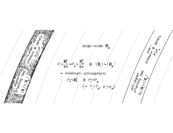
Figure 1: Embedded non-force-free underdense (dark) and overdense (bright) flux tubes running parallel to the large-scale background magnetic field (dotted lines). Direct pressure balance requires a minimum ambient atmosphere outside evacuated flux tubes determined solely by the background field $P_{\rm{e}}\sim{\bf{B}}_{\rm{e}}^{2}$, which gives a flux-tube pressure and density proportional to the ambient $P_{\rm{i}}\sim P_{\rm{e}}$, $\rho_{\rm{i}}\sim\rho_{\rm{e}}$, and temperature equal to it $T_{\rm{i}}=T_{\rm{e}}$.

For a small-scale magnetic field superposed on a stronger background field, Parker (1972) shows that equilibrium is possible only if the pattern of small-scale variations is uniform along the large-scale background field with ${\bf{B}}_{\rm{i}}\parallel{\bf{B}}_{\rm{e}}$. Field parallelism is consistent with coronal observations, which show fine filaments following the background field and tracing out its large-scale organization over their lengths (e.g. NK96, or see Sakurai & Uchida 1977). Flux conservation over the cross section of the embedded field then gives an internal field strength proportional to the external field strength

$${\bf{B}}_{\rm{i}}^{2}=(1+\beta){\bf{B}}_{\rm{e}}^{2},$$ (2)

for $\beta$ constant along the embedded field, with $\beta>0$ for aligned and $\beta<0$ for anti-aligned offsetting embedded fields. Strictly, the Parker (1972) parallelism of the embedded field is for an idealized straight background field. Limitations in the accuracy of the embedded-field parallelism are elaborated at the end of Section 4 and in Section 6.

Using Eq. (2) to eliminate ${\bf{B}}_{\rm{i}}^{2}$ from Eq. (1) gives

$$P_{\rm{e}}=\beta{{\bf{B}}_{\rm{e}}^{2}\over 8\pi}+P_{\rm{i}}.$$ (3)

Evacuation $P_{\rm{i}}=0$ in the strongest aligned embedded fields of largest $\beta$ seems natural as Lorentz-force-driven outflows cease when the equilibrium condition Eq. (1) is minimally met. Thus the atmospheric pressure relation may be written

$$P_{\rm{e}}=\beta_{\rm{c}}{{\bf{B}}_{\rm{e}}^{2}\over 8\pi},$$ (4)

with the pressure coefficient $\beta_{\rm{c}}=\beta$ for the overall strongest embedded fields over the globe. The gas pressure $P_{\rm{e}}$ for the minimum atmosphere everywhere outside embedded fields is proportional to the background magnetic pressure ${\bf{B}}_{\rm{e}}^{2}/(8\pi)$.

In an atmosphere $P_{\rm{e}}$ of given $\beta_{\rm{c}}$ from Eq. (4), embedded fields with aligned offsetting fields of weaker excess field strength $\beta<\beta_{\rm{c}}$ in Eq. (3) exhibit the positive internal pressure

$$P_{\rm{i}}=(1-{\beta\over\beta_{\rm{c}}})P_{\rm{e}},$$ (5)

so as the embedded field ranges in strength from $0<\beta\leq\beta_{\rm{c}}$, its internal pressure goes correspondingly from $P_{\rm{e}}>P_{\rm{i}}\geq 0$.

An embedded field with an anti-aligned offsetting magnetic field, as on the right in the drawing in Figure 1, must exhibit a reduced internal field strength ranging from $0\leq{\bf{B}}_{\rm{i}}^{2}<{\bf{B}}_{\rm{e}}^{2}$. Even though anti-aligned flux tubes may in principle exhibit a net reversed internal field with ${\bf{B}}_{\rm{i}}$ directed oppositely to ${\bf{B}}_{\rm{e}}$, the magnetic displacement pressure is always nonnegative with the minimum ${\bf{B}}_{\rm{i}}^{2}=0$. The realizable range of magnetic field strengths from $0\leq{\bf{B}}_{\rm{i}}^{2}<{\bf{B}}_{\rm{e}}^{2}$ corresponds to the range $-1\leq\beta<0$ in Eq. (2), giving the corresponding range of internal pressures $(1+1/\beta_{\rm{c}})P_{\rm{e}}\geq P_{\rm{i}}>P_{\rm{e}}$ from Eq. (5).

The full range of internal gas pressure for coronal flux tubes is from $0\leq P_{\rm{i}}\leq(1+1/\beta_{\rm{c}})P_{\rm{e}}$ as their field strengths range from $\beta_{\rm{c}}\geq\beta\geq-1$. With their internal pressures everywhere proportional to the external ambient from Eq. (5), their hydrostatic temperatures must be the same as the local ambient $T_{\rm{i}}=T_{\rm{e}}$ from the hydrostatic relation, i.e. Eq. (37) in Section 7. Then by the perfect gas law, their internal densities must be proportional $\rho_{\rm{i}}\sim\rho_{\rm{e}}$. In the limiting strongest stable atmosphere $\beta_{\rm{c}}=1$, flux tubes range in density from evacuated to two times the ambient, which is what is seen in the solar corona shown in Figures 14 and 15 of NK96.

With a global distribution of flux tubes of similar strength, there will only be one atmospheric coupling constant $\beta_{\rm{c}}$ for the large-scale global atmosphere. The strength of the flux tubes might really be fixed by the limit for global magnetic stability rather than by any particular property intrinsic to flux tubes. Active-region magnetic fields are very much stronger than quiet-sun fields but of small global surface areal coverage. Energized only by local subsurface convective motions, they probably cannot raise the whole surrounding coronal atmosphere up to their magnetic pressures, and so must tend to relax to near force free for pressure balance with the surrounding quiet corona. Comparisons between solar coronal density and extrapolated magnetic field strength do suggest that the solar corona has a gas pressure comparable to the magnetic pressure with $\beta_{\rm{c}}\simeq 1$ in Eq. (4) outside active regions (Gary, 2001).

Active-region temporally varying or average components are known to contribute only a small fraction to the total solar coronal X-ray emission (Orlando et al., 2004; Argiroffi et al., 2008). However it seems possible to include their physics in an overall coronal picture. Solar active regions appear to consist mainly of closed low-lying field lines with a background magnetic field that is very much locally enhanced and separated, even possibly abruptly so, from the surrounding quiet corona. The active-region background field contains its own embedded current-carrying fields, which must be near force free and described by the same pressure balance Eq. (1), but with gas pressures inside and outside $P_{\rm{iar}}$ and $P_{\rm{e}}$ small compared to the magnetic pressures ${\bf{B}}_{\rm{iar}}^{2}/(8\pi)$ and ${\bf{B}}_{\rm{ear}}^{2}/(8\pi)$, that is with ${\bf{B}}_{\rm{iar}}^{2}\simeq{\bf{B}}_{\rm{ear}}^{2}$ or $|\beta|\ll 1$ in Eq. (2). Active-region current-carrying fields may reach evacuation $P_{\rm{iar}}=0$ even though they have an internal magnetic field strength only a little greater than that of their embedding magnetic field ${\bf{B}}_{\rm{iar}}^{2}\gtrsim{\bf{B}}_{\rm{ear}}^{2}$, giving a coronal beta $\beta_{\rm{car}}$ that is very small in Eq. (4), distinctly less than that of the quiet sun $\beta_{\rm{car}}\ll\beta_{\rm{c}}\lesssim 1$.

4 Embedded Form

As a more comprehensive approach, the localized current-carrying magnetic field is decomposed into transverse and longitudinal components from a main vector axis as

$${\bf{B}}={\bf\nabla}{\bf\times}(\check{a}{\bf\Omega})+\check{b}{\bf\Omega},$$ (6)

where the functions marked by an over-check are called the ‘constituent functions’ of the embedded field, which vary only in its vicinity. For a localized embedded field, the constituent functions asymptotically become $\check{a}\rightarrow 0$ and $\check{b}\rightarrow\check{b}_{\rm{e}}$ a constant far from the embedded field.

The vector axis ${\bf\Omega}$ for the magnetic field is commonly taken as a constant coordinate direction ${\bf\Omega}\rightarrow{\bf\nabla}z$, which leads to the well-known 2D MHD GS solutions developed in the literature in different ways in a number of publications (Lüst & Schlüter, 1954, 1957; Chandrasekhar, 1956; Grad & Rubin, 1958; Shafranov, 1958). Greater flexibility is allowed by taking the vector axis ${\bf\Omega}$ to be a general Euler coordinate or flux surface for the magnetic field (e.g. D’haeseleer et al. 1991). With the continuity of the magnetic field

$${\bf\nabla}{\bf\cdot}{\bf{B}}=0,$$ (7)

it follows

$${\bf\nabla}{\bf\cdot}(\check{b}{\bf\Omega})=0,$$ (8)

and applying Gauss’ theorem, the longitudinal magnetic flux, the cross-sectional areal integral of $\check{b}{\bf\Omega}$, must be conserved over every perpendicular surface within any given set of field lines. Taking the flux surface ${\bf\Omega}$ to be a conservative vector field

$${\bf\nabla}{\bf\cdot}{\bf\Omega}=0,$$

consistent with its usage as an Euler coordinate, then gives a conserved longitudinal constituent function $\check{b}$ along the flux surface ${\bf\Omega}$

$${\bf\Omega}{\bf\cdot}{\bf\nabla}\check{b}=0.$$ (9)

The transverse magnetic flux is taken to be similarly conserved

$${\bf\nabla}{\bf\cdot}(\check{a}{\bf\Omega})=0,{\rm\ giving}\quad{\bf\Omega}{\bf\cdot}{\bf\nabla}\check{a}=0,$$ (10)

for a constituent function $\check{a}$ constant along flux-surface lines. The transverse constraint is a gauge choice, the Coulomb gauge, which simplifies the current density ${\bf{J}}$ and Lorentz force ${\bf{F}}$. There appears to be no possibility for finding explicit isotropic solutions otherwise, as many dot products ${\bf\Omega}{\bf\cdot}{\bf\nabla}\check{a}$ arise in independent ways in expansions of the Lorentz force. The magnetic-field transverse and longitudinal fluxes are conserved, that is the areal integrals of $\check{a}{\bf\Omega}$ and $\check{b}{\bf\Omega}$ over every cross section within any given set of field lines, whereas the constituent function remapped values $\check{a}$ and $\check{b}$ remain constant even as the field spreads out or changes shape.

The current density ${\bf{J}}=\genfrac{}{}{}{1}{c}{4\pi}{\bf\nabla}{\bf\times}{\bf{B}}$ with a conserved transverse constituent function $\check{a}$ from Eq. (10) is written

$${\bf{J}}={c\over 4\pi}\left({\bf\nabla}{\bf\times}(\check{b}{\bf\Omega})-{\bf\nabla}^{2}(\check{a}{\bf\Omega})\right),$$ (11)

leading to a Lorentz force ${\bf{F}}=\genfrac{}{}{}{1}{1}{c}{\bf{J}}{\bf\times}{\bf{B}}$, which expands into four cross-product terms

$$\begin{split}&{\bf{F}}={1\over 4\pi}\biggl{(}\bigl{\{}({\bf\nabla}{\bf\times}(\check{b}{\bf\Omega})){\bf\times}({\bf\nabla}{\bf\times}(\check{a}{\bf\Omega}))\bigr{\}}_{1}+\bigl{\{}({\bf\nabla}{\bf\times}(\check{b}{\bf\Omega})){\bf\times}\check{b}{\bf\Omega}\bigr{\}}_{2}\\ &-\bigl{\{}({\bf\nabla}^{2}(\check{a}{\bf\Omega})){\bf\times}({\bf\nabla}{\bf\times}(\check{a}{\bf\Omega}))\bigr{\}}_{3}-\bigl{\{}({\bf\nabla}^{2}(\check{a}{\bf\Omega})){\bf\times}{\bf\nabla}(\check{b}{\bf\Omega})\bigr{\}}_{4}\biggr{)}.\end{split}$$ (12)

Terms in the expression are numbered by subscripts for later identification.

It is convenient to write the Lorentz force as a sum of three parts with distinct physical properties, which are studied separately, as

$$\begin{split}{\bf{F}}={\bf{F}}_{\rm{e}}+{\bf{F}}_{\rm{i0}}+{\bf{F}}_{\rm{i1}},\end{split}$$ (13)

a global part ${\bf{F}}_{\rm{e}}$ that does not die off away from the embedded field, and local parts ${\bf{F}}_{\rm{i0}}$ and ${\bf{F}}_{\rm{i1}}$ that do. All of the Lorentz-force terms in the expansion in Eq. (12) that contain the constituent function $\check{a}$ or a derivative of $\check{b}$ do die off and are local, which leaves only one vector cross product out of the second term that does not die off locally, written

$${\bf{F}}_{\rm{e}}={\check{b}^{2}\over 4\pi}({\bf\nabla}{\bf\times}{\bf\Omega}){\bf\times}{\bf\Omega}.$$ (14)

With the flux surface ${\bf\Omega}$ becoming asymptotically parallel to the background field as it must in Eq. (6),

$${\bf{B}}_{\rm{e}}=\check{b}_{\rm{e}}{\bf\Omega},$$ (15)

and the global Lorentz force becomes consistently the Lorentz force due to a background non-potential magnetic field ${\bf{B}}_{\rm{e}}$

$${\bf{F}}_{\rm{e}}={1\over 4\pi}({\bf\nabla}{\bf\times}{\bf{B}}_{\rm{e}}){\bf\times}{\bf{B}}_{\rm{e}}.$$ (16)

The remaining terms in the expanded Lorentz force are grouped into a part ${\bf{F}}_{\rm{i0}}$ where the flux surface ${\bf\Omega}$ appears undifferentiated, and into a part ${\bf{F}}_{\rm{i1}}$ otherwise. As long as the scale of variation of the flux surface $H_{\Omega}=H_{\rm{Be}}$ is large compared to a characteristic scale of variation in the current-carrying field $d$, the derivatives of the basis vector will be relatively small compared to those of the constituent functions, giving ${\bf{F}}_{\rm{i1}}$ of relative order $d/H_{\rm{Be}}$ compared to ${\bf{F}}_{\rm{i0}}$. The more-significant-order Lorentz-force part ${\bf{F}}_{\rm{i0}}$ is expanded

$${\bf{F}}_{\rm{i0}}={{\bf\Omega}^{2}\over 4\pi}\biggl{(}\bigl{\{}{\bf\nabla}\check{b}{\bf\times}{\bf\nabla}\check{a}\bigr{\}}_{1}-\bigl{\{}\check{b}{\bf\nabla}\check{b}\bigr{\}}_{2}-\bigl{\{}{\bf\nabla}^{2}\check{a}{\bf\nabla}\check{a}\bigr{\}}_{3}\biggr{)},$$ (17)

applying vector identities to the respective terms in Eq. (12) straightforwardly, with the fourth term disappearing as it reduces to a cross product between two vectors both parallel to ${\bf\Omega}$. The usual notational convention is adopted that differential operators, as gradient ${\bf\nabla}$, Laplacian ${\bf\nabla}^{2}$, or tensorial $\partial_{\imath}={\bf\nabla}_{\imath}$, have precedence over multiplication, operating only on their first following variable.

The MHD approximation with an isotropic pressure is commonly taken to be applicable even in very low-density astrophysical conditions, as mixing processes, especially Coulomb scattering, tend to isotropize the gas pressure still on scales small compared to the magnetic structure. The equilibrium magnetic flux is thus expected to have a spatial distribution with minimal anisotropy in its Lorentz force. In ideal cases, like the static GS straight field geometry, isotropic pressure solutions are found, but anisotropic effects cannot be avoided in more usual plasma problems (e.g. Bellan 2008; Biskamp 2008). The external factor ${\bf\Omega}^{2}$ in the expression for the local Lorentz force in Eq. (17) represents a slow global variation that becomes identified with external forces in the separation of the gas pressure into globally and locally varying relations, as described in Section 5 and Appendix B. For local isotropy, the ratio ${\bf{F}}/{\bf\Omega}^{2}$ is left equated to the gradient of a scalar pressure.

A Lorentz force that is locally isotropic with ${\bf\nabla}{\bf\times}({\bf{F}}/{\bf\Omega}^{2})=0$ is sought, at least as a weak constraint that may not always be possible to satisfy exactly. The second term in Eq. (17) always vanishes under the curl ${\bf\nabla}{\bf\times}({\check{b}}{\bf\nabla}{\check{b}})={\bf\nabla}{\bf\times}({\bf\nabla}{\check{b}}^{2})/2=0$. The vanishing of the third term under the curl ${\bf\nabla}{\bf\times}({\bf\nabla}^{2}\check{a}{\bf\nabla}\check{a})={\bf\nabla}({\bf\nabla}^{2}\check{a}){\bf\times}{\bf\nabla}\check{a}=0$, requires that the vectors be everywhere parallel ${\bf\nabla}\check{a}\parallel{\bf\nabla}({\bf\nabla}^{2}\check{a})$. The three underlying Jacobian $2\times 2$ determinants in the cross product are zero (with at least one nontrivially so), implying the functional dependency ${\bf\nabla}^{2}\check{a}=({\bf\nabla}^{2}\check{a})[\check{a}]$ or the inverse $\check{a}=\check{a}[{\bf\nabla}^{2}\check{a}]$, which may be multivalued dependencies. For clarity in the subtle functional relations, square braces are used throughout to denote a functional dependence.

As both $\check{a}$ and $\check{b}$ are constant in the direction of the flux surface ${\bf\Omega}$ by Eqs. (10) and (9), their gradients are both perpendicular to ${\bf\Omega}$, and the cross product, the first term in Eq. (17), parallel ${\bf\nabla}\check{a}{\bf\times}{\bf\nabla}\check{b}\parallel{\bf\Omega}$, so the cross product is unidirectional locally with ${\bf\Omega}\parallel{\bf\nabla}z$. For the curl of the cross product to vanish, the term itself must be the gradient of a scalar function as ${\bf\nabla}\check{a}{\bf\times}{\bf\nabla}\check{b}={\bf\nabla}f[z]=(df/dz){\bf\nabla}z$ for $f[z]$ a function of a single coordinate $z$. The cross product ${\bf\nabla}\check{a}{\bf\times}{\bf\nabla}\check{b}=(df/dz){\bf\nabla}z$ is a function of $z$ alone, but as the functions $\check{a}$ and $\check{b}$ are bounded in their variations away from the center of the embedded field, they must exhibit functional dependencies perpendicular to ${\bf\nabla}z$, as so must any nonzero cross product ${\bf\nabla}\check{a}{\bf\times}{\bf\nabla}\check{b}$. Variations perpendicular to $z$ in the cross product contradict its unidirectional requirement, so bounded solutions are only possible with the vanishing of the cross product itself everywhere ${\bf\nabla}\check{a}{\bf\times}{\bf\nabla}\check{b}=0$, which necessitates the multivalued functional dependencies $\check{b}=\check{b}[\check{a}]$ or the inverse $\check{a}=\check{a}[\check{b}]$.

The continuity of $\check{a}$ in Eq. (10) and $\check{b}$ in Eq. (9) are consistent with, though not necessarily implying, the functional constraint $\check{b}=\check{b}[\check{a}]$. Without the continuity of $\check{a}$ as a gauge choice, the functional constraint $\check{b}=\check{b}[\check{a}]$ cannot be satisfied. The form of the solution described here is only consistent with the choice of gauge.

Applying the functional constraints ${\bf\nabla}^{2}\check{a}=({\bf\nabla}^{2}\check{a})[\check{a}]$ and $\check{b}=\check{b}[\check{a}]$ to Eq. (17) gives

$${\bf{F}}_{\rm{i0}}=-{{\bf\Omega}^{2}\over 4\pi}\left(({\bf\nabla}^{2}\check{a})[\check{a}]+{1\over 2}{d\check{b}^{2}\over d\check{a}}\right){\bf\nabla}\check{a},$$ (18)

which resembles the classical 2D GS Lorentz force for straight geometries, but now written for 3D Laplacian and constituent functions.

The remaining smaller-order local Lorentz-force ${\bf{F}}_{\rm{i1}}$ reduces as elaborated in Appendix A. It vanishes in a potential flux surface ${\bf\Omega}$ in Cartesian current-sheet solutions to give the purely isotropic Lorentz force written in Eq. (18). Otherwise a small-order anisotropic Lorentz force $F_{\rm{i1}}$ of order ${\bf{B}}_{\rm{e}}^{2}/H_{\rm{Be}}$ arises. Compared to the isotropic Lorentz force $F_{\rm{i0}}$ from Eq. (18), which is of order ${\bf{B}}_{\rm{e}}^{2}/d$, the anisotropic Lorentz force has the small relative order $d/H_{\rm{Be}}$, for $d$ the main scale of variation in the current-carrying field.

With a vanishing transverse field in the current-carrying field away from its center, asymptotic parallelism of the embedded and background fields away from the embedded field, as in Eq. (15), is an implicit feature of the magnetic-field specification Eq. (6). However that field specification is not the most general possible. A vector field can be added to Eq. (6) as a third independent degree of freedom, as with the addition of a potential field in a Helmholtz decomposition (Morse & Feshbach 1953, Section 13.1; Parker 1979, p. 542). It is sometimes possible to redefine the terms in the superposition to give back the form for the magnetic field in Eq. (6). Otherwise the background magnetic field will not be parallel to the flux surface ${\bf{B}}_{\rm{e}}\not\parallel{\bf\Omega}$, but then new anisotropic terms are also added to the Lorentz force of most-significant order, as is straightforwardly demonstrated. These lead to anisotropic Lorentz forces of relative order the angular deviation between the flux surface and background field $d/H_{\rm{Be}}$.

The scale height for a solar potential spherical-harmonic of degree $\ell=2$ is $H_{\rm{Be}}=R_{\odot}/(\ell+2)=174$ Mm. With flux tubes of diameter $d_{\rm{cc}}\simeq 0.7$ Mm from the NK96 eclipse observation, $d_{\rm{cc}}/H_{\rm{Be}}\simeq 4$E$-3$, with still finer flux tubes likely present in the lower corona as are inferred farther out. In thin-sheathed flux tubes embedded in a background potential field, which are described in Section 6, the characteristic scale of variation is the sheath thickness $d=d_{\rm{sh}}$, which may be much smaller than the flux-tube diameter. The anisotropic Lorentz forces are correspondingly smaller by the factor $d_{\rm{sh}}/d_{\rm{cc}}$, and confined to the sheath.

5 Solution Separability

This work develops an overall equilibrium solution strategy for embedded current-carrying fields based upon the separation of the MHD equations into independent global and local relations like what is advanced in N04, but now shown to be applicable in more wide-ranging circumstances, as with flows and temperature variations. The MHD pressure balance is expressed

$${\bf\nabla}P+{P\over H_{\rm{s}}g[R]}{D{\bf{u}}\over Dt}+{P\over H_{\rm{s}}}{\bf\nabla}R={1\over 4\pi}({\bf\nabla}{\bf\times}{\bf{B}}){\bf\times}{\bf{B}},$$ (19)

with the gas pressure $P$, static pressure scale height $H_{\rm{s}}$, flow vector ${\bf{u}}$, inward gravitational acceleration $g[R]$, with the radial coordinate $R$ from the gravitating center, and total time derivative for the flow field $D{\bf{u}}/Dt=\partial{\bf{u}}/\partial t+{\bf{u}}{\bf\cdot}{\bf\nabla}{\bf{u}}$. Time derivatives are retained in the global ambient equation to explore near equilibrium effects, but the steady equilibrium with zero time derivatives is of principle interest. The density $\rho$ is eliminated in favor of the static pressure scale height $H_{\rm{s}}$ with $P/H_{\rm{s}}=\rho g[R]$. Supposing a perfect gas with $P=\rho kT/\bar{m}$ gives $H_{\rm{s}}=kT/(\bar{m}g[R])$ proportional to the temperature $T$, with Boltzmann’s constant $k$, and the mean particle mass $\bar{m}$.

The equations are completed with the continuity of the flow field and the magnetic-induction equation for a fully conductive plasma

$${\partial\rho\over\partial t}+{\bf\nabla}{\bf\cdot}(\rho{\bf{u}})=0,\quad\quad{\partial{\bf{B}}\over\partial t}={\bf\nabla}{\bf\times}\left({\bf{u}}{\bf\times}{\bf{B}}\right).$$ (20)

Upper-case symbols $(R,\Theta,\Phi)$ are used throughout to denote the global spherical large-scale, e.g. helio-, stellar-, planetary-, or galactic-centered system, a convention common in astrophysics. Lower-case symbols are reserved for the local coordinates of the embedded field, as Cartesian $(x,y,z)$, or cylindrical $(r,\phi,z)$.

In the present section, the background magnetic field is assumed to be potential, and the static scale height $H_{\rm{s}}$ or temperature $T$, and flow field ${\bf{u}}$ taken to be varying globally without showing any systematic variations near embedded fields. Effects of a non-potential background field, locally changing temperatures and flows, radiation and cosmic-ray pressures, or viscosity are of interest in this work. A general strategy for including other physical processes is discussed at the end of this section and developed in Appendix B.

Multiple terms in the MHD pressure balance Eq. (19) are encorporated into a single integrating factor $\Pi$ with the substitution

$$P=\check{P}\exp\left[-\Pi\right],$$ (21)

introducing the relative gas pressure $\check{P}$, which varies near embedded fields, but is constant everywhere outside, and with $\Pi$ varying only globally. Taking the gradient leads to

$${\bf\nabla}P+P{\bf\nabla}\Pi=\exp\left[-\Pi\right]{\bf\nabla}\check{P},$$ (22)

which is a perfect template matching in its left and right sides those of the MHD Eq. (19). The scalar integrating factor $\Pi$ acts as an isotropic pressure whose gradient must balance the total of all the vector forces in the global field outside embedded fields.

Laying the template Eq. (22) over the MHD Eq. (19) gives for the integrating factor from the equated left-sides

$${\bf\nabla}\Pi={1\over H_{\rm{s}}g[R]}{D{\bf{u}}\over Dt}+{1\over H_{\rm{s}}}{\bf\nabla}R,$$ (23)

and the pressure relation from the equated right sides

$$\exp[-\Pi]{\bf\nabla}\check{P}={1\over 4\pi}({\bf\nabla}{\bf\times}{\bf{B}}){\bf\times}{\bf{B}},$$ (24)

which is expanded

$$\exp[-\Pi]{\bf\nabla}\check{P}=-{{\bf\Omega}^{2}\over 4\pi}\left\{({\bf\nabla}^{2}\check{a})[\check{a}]{\bf\nabla}\check{a}+{1\over 2}{d\check{b}^{2}\over d\check{a}}{\bf\nabla}\check{a}\right\},$$ (25)

for the magnetic field from Eq. (6) using the Lorentz force ${\bf{F}}={\bf{F}}_{\rm{i0}}$ from Eq. (18), taking for simplicity the global and small-order parts ${\bf{F}}_{\rm{e}}={\bf{F}}_{\rm{i1}}=0$, relevant for the assumed potential background magnetic field. Even in a potential background field, additional small terms are introduced into the locally varying part in curly braces with a nonvanishing ${\bf{F}}_{\rm{i1}}$ as in non-Cartesian solutions, or with ${\bf{F}}_{\rm{e}}$ as for small potential-field deviations in local current-carrying-field solutions as elaborated in Section 6. In a non-potential background magnetic field, with flows, or with temperature variations, additional principle-order effects enter into the locally varying part. Some elaboration of additional effects are described at the end of this section and in Appendix B.

In Eq. (25), all the terms in the integrating factor $\Pi$ and the flux surface ${\bf\Omega}^{2}$ vary globally away from and continuously across embedded fields, whereas the gradient of the relative gas pressure ${\bf\nabla}\check{P}$ and all the terms in curly braces on the right side are local to the embedded field. Thus the separation is suggested

$${\bf\nabla}\check{P}=-{1\over 4\pi}\left(({\bf\nabla}^{2}\check{a})[\check{a}]+{1\over 2}{d\check{b}^{2}\over d\check{a}}\right){\bf\nabla}\check{a},$$ (26)

for the local field, and

$$\exp[-\Pi]={\bf\Omega}^{2},$$ (27)

for the global field. An arbitrary separation constant is introduced, which has allowed the factor $4\pi$ to be moved into Eq. (26) to give the local relation the exact 2D GS equation form in Gaussian units.

The global relation Eq. (27) is recast into a more familiar form as an MHD pressure relation just for the global field. Taking the natural log of both sides and operating with the gradient gives

$${\bf\nabla}\Pi=-{\bf\nabla}\ln[{\bf\Omega}^{2}],$$

then substituting the integrating factor from Eq. (23) leaves

$${\bf\nabla}\ln[{\bf\Omega}^{2}]+{1\over H_{\rm{s}}g[R]}{D{\bf{u}}\over Dt}+{1\over H_{\rm{s}}}{\bf\nabla}R=0.$$ (28)

A given global distribution for the flux surface ${\bf\Omega}^{2}$ determines the static scale height $H_{\rm{s}}$ or temperature, and flow field ${\bf{u}}$. The relation is indistinguishable from the MHD pressure equation for a global potential magnetic field. Substituting with the ambient gas pressure defined in terms of the flux surface $P_{\rm{e}}=\beta_{\rm{c}}\check{b}_{\rm{e}}^{2}{\bf\Omega}^{2}/(8\pi)$, and taking the product $\beta_{\rm{c}}\check{b}_{\rm{e}}^{2}$ to be a global constant gives

$${\bf\nabla}P_{\rm{e}}+{P_{\rm{e}}\over H_{\rm{s}}g[R]}{D{\bf{u}}\over Dt}+{P_{\rm{e}}\over H_{\rm{s}}}{\bf\nabla}R=0,\quad{\rm{with}}\quad P_{\rm{e}}=\beta_{\rm{c}}{{\bf{B}}_{\rm{e}}^{2}\over 8\pi},$$ (29)

equating the flux surface to the ambient magnetic field away from embedded fields ${\bf\Omega}={\bf{B}}_{\rm{e}}/\check{b}_{\rm{e}}$ in the coupling condition on the right.

The coupled equilibrium agrees with what was found with the direct pressure balance of Eq. (4) in Section 3. The external asymptotic longitudinal constituent function $\check{b}_{\rm{e}}$ must be constant along flux tubes, like the constituent function $\check{b}$ itself by the continuity relation (9), and needs to be constant between flux tubes too for the background field to be everywhere consistently defined. The interconnectedness of flux tubes over the quiet corona thus suggests that $\check{b}_{\rm{e}}$ must be a large-scale global constant, giving a constant coupling coefficient $\beta_{\rm{c}}$ for their product to be constant, which is consistent with the assumption from Section 3 that flux tubes must be similarly conditioned globally. The model can accommodate solar active regions with a gas pressure $P_{\rm{e}}$ that remains continuous crossing from the quiet sun into the active region, with beta $\beta_{\rm{c}}$ very much reduced and the background field ${\bf{B}}_{\rm{e}}$ correspondingly stronger.

As described in Section 6 and in Appendix B, in equilibrium solutions, with flows or temperature variations in embedded fields, or in a non-potential background field, terms add to the Lorentz force, and so to the curly braces in Eq. (25) and to the local equilibrium in Eq. (26). However there is only one atmosphere, so an atmospheric coupling relation like Eq. (27), must have a unique global functional form even with a mixture of embedded current-carrying fields with their various and differing internal consistencies. Added Lorentz-force terms exhibit specific globally varying properties, but a most-significant-order Lorentz force Eq. (18) always appears with its single globally varying part ${\bf\Omega}^{2}$ factored externally. Thus whatever the mixture of current-carrying fields, the gas-pressure coupling with ${\bf\Omega}^{2}$ in Eq. (27) appears to be the only reasonable universally consistent possibility, and so the coupled equilibrium of Eq. (29). Individual embedded fields with differing internal contributions must adjust within to find equilibrium balance along their lengths with any overall average-defined background atmosphere.

6 Local Equilibrium

The relative gas pressure $\check{P}$ varies only locally to the embedded field, defining its cross-sectional profile relative to the local ambient gas pressure. It is constant across a force-free embedded field, but exhibits a fractional dip in the center of a non-force-free embedded field of increased field strength, or a fractional bump in one of decreased field strength.

The relative gas pressure $\check{P}$ must be conserved along the current-carrying field lines for the local Eq. (26) to be satisfied. Its gradient is parallel to the transverse constituent function ${\bf\nabla}\check{P}\parallel{\bf\nabla}\check{a}$, and so must satisfy the functional relation $\check{P}=\check{P}[\check{a}]$. With the continuity of $\check{a}$ along the lines of the flux surface from Eq. (10), then

$${\bf\Omega}{\bf\cdot}{\bf\nabla}\check{P}[\check{a}]=\left({d\check{P}\over d\check{a}}\right){\bf\Omega}{\bf\cdot}{\bf\nabla}\check{a}=0,{\rm\ or}\quad{\bf{B}}_{\rm{e}}{\bf\cdot}{\bf\nabla}\check{P}=0,$$ (30)

using the flux-surface background-field parallelism ${\bf\Omega}\parallel{\bf{B}}_{\rm{e}}$ in the rightmost equality. The constituent functions are normalized so that $\check{a}$ and $\check{b}$ are actual magnetic field strengths and $\check{P}$ an actual gas pressure at a reference height where $|{\bf\Omega}|^{2}=1$. Away from that height, the magnetic-field constituent functions $\check{a}$ and $\check{b}$ multiplied by the flux surface $|{\bf\Omega}|$ give the actual transverse and longitudinal field fluxes, and the relative gas pressure $\check{P}$ multiplied by ${\bf\Omega}^{2}$ the actual gas pressure.

With the functional constraint $\check{P}=\check{P}[\check{a}]$, the local equilibrium relation Eq. (26) takes the familiar form of the GS equation

$$-{1\over 4\pi}{\bf\nabla}^{2}\check{a}={d\over d\check{a}}\left(\check{P}+{1\over 8\pi}\check{b}^{2}\right),$$ (31)

but here written for 3D spatial functions. The GS relation is essentially an expression of the conservation of the total gas-plus-magnetic pressure in the vicinity of the embedded field. The constituent function can always be written $\check{a}=\check{a}[\xi]$ with an intermediate variable $\xi$, which is a function of the embedded-field coordinates, e.g. Cartesian $\xi=\xi[x,y,z]$ or cylindrical $\xi=\xi[r,\phi,z]$. With the intermediate functional dependence, the Laplacian is expanded

$${\bf\nabla}^{2}(\check{a}[\xi])={d^{2}\check{a}\over d\xi^{2}}|{\bf\nabla}\xi|^{2}+{d\check{a}\over d\xi}{\bf\nabla}^{2}\xi,$$ (32)

and with $\check{b}=\check{b}[\check{a}[\xi]]=\check{b}[\xi]$, and $\check{P}=\check{P}[\check{a}[\xi]]=\check{P}[\xi]$, the GS Eq. (31) becomes

$${d\over d\xi}\left(\check{P}[\xi]+{1\over 8\pi}\check{b}[\xi]^{2}\right)+{1\over 8\pi}{d\over d\xi}\left(d\check{a}\over d\xi\right)^{2}|{\bf\nabla}\xi|^{2}+{1\over 4\pi}\left({d\check{a}\over d\xi}\right)^{2}{\bf\nabla}^{2}\xi=0,$$ (33)

applying the chain rule. Integrating in $\xi$ between any $\xi_{0}$ and $\xi_{1}$ yields

$$\check{P}[\xi]+{1\over 8\pi}\check{b}[\xi]^{2}+{1\over 8\pi}\left({d\check{a}\over d\xi}\right)^{2}+{1\over 4\pi}\int_{\xi_{0}}^{\xi_{1}}{\left({d\check{a}\over d\xi}\right)^{2}{\bf\nabla}^{2}\xi d\xi}={\rm{constant}},$$ (34)

taking $|{\bf\nabla}\xi|^{2}=1$, which is relevant for Cartesian current-sheet and cylindrical axisymmetric (not azimuthally varying) flux-tube solutions. The remaining integral can be seen to represent an added pressure due to magnetic field tension in the current-carrying field.

In local embedded-field equilibria of interest, internal magnetic field tension is negligible. For current-sheets, $|{\bf\nabla}\xi|^{2}=1$ and ${\bf\nabla}^{2}\xi=0$, and the added integral term in Eq. (34) disappears. The condition ${\bf\nabla}^{2}\xi\rightarrow 0$ is asymptotic for thin-sheathed flux tubes. Multiplying through by the flux surface ${\bf\Omega}^{2}$ renormalizes the constant constituent functions along their paths through the corona, giving a conserved total pressure

$$P+{{\bf{B}}^{2}\over 8\pi}={\rm{constant}},$$ (35)

around every spatial locale, substituting using $\check{P}=P/{\bf\Omega}^{2}$ from Eqs. (21) and (27), with ${\bf{B}}^{2}=((d\check{a}/d\xi)^{2}+\check{b}^{2}){\bf\Omega}^{2}$ from Eq. (6), and ignoring the relatively small derivatives of the flux surface ${\bf\Omega}$. Such a conserved total pressure was assumed in Eq. (1) for direct pressure balance in the vicinity of current-carrying fields in Section 3. A significant pressure offset from a direct pressure balance within the current-carrying field is possible due to the added tension term in Eq. (34), which may be relevant for flux tubes with inhomogeneous internal structure as below the coronal base, as described further below.

Near force-free current-carrying fields follow the same relations but with relatively small gas-pressure changes compared to magnetic-pressure values, i.e. $|P_{\rm{i}}-P_{\rm{e}}|\ll{\bf{B}}_{{\rm{e}}}^{2}/(8\pi)$ and ${\bf{B}}_{\rm{i}}^{2}/(8\pi)$. Pure force-free fields exhibit current-density magnetic-field parallelism ${\bf{J}}\parallel{\bf{B}}$ or ${\bf\nabla}{\bf\times}{\bf{B}}=\alpha{\bf{B}}$ for $\alpha$ constant along field lines. Substituting ${\bf{B}}$ from Eq. (6) and ${\bf\nabla}{\bf\times}{\bf{B}}$ from Eq. (11) with ${\bf\Omega}$ a constant vector shows that $\alpha=d\check{b}/d\check{a}$. In the force-free limit, the derivative vanishes $d\check{P}/d\check{a}=0$ in the GS Eq. (31) meaning both $P$ and ${\bf{B}}^{2}$ are separately constant in every locale in Eq. (35), results consistent with what is expected for a vanishing Lorentz force in force-free fields.

GS equilibria are explored by looking for functions $\check{a}=\check{a}[\xi]$ that satisfy the functional constraint ${\bf\nabla}^{2}\check{a}=({\bf\nabla}^{2}\check{a})[\check{a}]$. The functional constraint $\check{b}=\check{b}[\check{a}]$ limits the choices for $\check{b}$ for a given spatial function $\check{a}$, but the constraint ${\bf\nabla}^{2}\check{a}=({\bf\nabla}^{2}\check{a})[\check{a}]$ is a template for the GS Eq. (31) itself and defines the allowed functional forms for $\check{a}$. Given a spatial dependence $\check{a}=\check{a}[\xi]$, as long as ${\bf\nabla}^{2}\check{a}=({\bf\nabla}^{2}\check{a})[\xi]$, it can be seen that ${\bf\nabla}^{2}\check{a}=({\bf\nabla}^{2}\check{a})[\check{a}]$. The derivatives $d^{2}\check{a}/d\xi^{2}$ and $d\check{a}/d\xi$ in Eq. (32) are always functions of $\xi$ alone, so there is always complete freedom in choosing the outer function $\check{a}[\xi]$. However with an arbitrary coordinate dependence in $\xi$, the derivative factors $|{\bf\nabla}\xi|^{2}$ and ${\bf\nabla}^{2}\xi$ need not be functions of $\xi$ alone.

Many useful continuous functions for $\check{a}[\xi]$ come to mind, like some which have an explicit inverse $\xi=\xi[\check{a}]$, as a Gaussian $\check{a}[\xi]=\check{a}_{\rm{i}}\exp[-\xi^{2}]$ for $\check{a}_{\rm{i}}$ its central internal $\xi=0$ value, with its double-valued inverse $\xi[\check{a}]=\pm(\ln[\check{a}/\check{a}_{\rm{i}}])^{1/2}$, or the smooth cutoff $\check{a}[\xi]=\check{a}_{\rm{i}}/(1+\exp[\xi])$ with its single-valued inverse $\xi[\check{a}]=\ln[\check{a}/\check{a}_{\rm{i}}-1]$. However the inverse need not be explicit to give an allowed outer function $\check{a}[\xi]$, as with a sinc function $\check{a}[\xi]=\sin[\xi]/\xi$, with its multivalued transcendental inverse $\xi[\check{a}]$.

Two of the 13 geometries separable under the Laplacian operator (Moon & Spencer 1971, §1) are mainly of relevance for embedded current-carrying fields: the Cartesian $(x,y,z)$ current sheet in a background field with 1D symmetry as in a linear arcade, and the cylindrical $(r,\phi,z)$ flux tube in a background field with 2D symmetry around the flux-tube center. Other forms such as spherical arise too as when considering embedded plasmoids.

In straight field geometries with ${\bf\Omega}\rightarrow z$, for variations perpendicular to $z$ across a Cartesian current sheet $\xi\rightarrow x$, the derivative factors in Eq. (32) are $|{\bf\nabla}\xi|^{2}=1$ and ${\bf\nabla}^{2}\xi=0$. For radial variations in a cylindrical flux tube constant in $z$, $\xi\rightarrow r$, corresponding to a twisted magnetic field, the derivative factors become $|{\bf\nabla}\xi|^{2}=1$ and ${\bf\nabla}^{2}\xi=1/r=1/\xi$. In both cases $|{\bf\nabla}\xi|^{2}=(|{\bf\nabla}\xi|^{2})[\xi]$ and ${\bf\nabla}^{2}\xi=({\bf\nabla}^{2}\xi)[\xi]$, so these geometries always satisfy the functional constraint ${\bf\nabla}^{2}\check{a}=({\bf\nabla}^{2}\check{a})[\check{a}]$ and the GS Eq. (31) with any continuous outer function $\check{a}[\xi]$.

A nonaxisymmetric flux tube with purely azimuthal variations $\xi\rightarrow\phi$ in a straight field geometry exhibits derivatives $|{\bf\nabla}\xi|^{2}=1/r^{2}$ and ${\bf\nabla}^{2}\xi=0$, giving ${\bf\nabla}^{2}(\check{a}[\xi])$ a residual $r$ dependence, which precludes the functional dependence $|{\bf\nabla}\xi|^{2}=(|{\bf\nabla}\xi|^{2})[\xi]$, and so the isotropy constraint ${\bf\nabla}^{2}\check{a}=({\bf\nabla}^{2}\check{a})[\check{a}]$ is not satisfied. However straight-field nonaxisymmetric solutions can be built-up based upon the complex $\xi=x+iy$ that do satisfy the functional dependencies giving ${\bf\nabla}^{2}\check{a}=({\bf\nabla}^{2}\check{a})[\check{a}]$. These lead to azimuthally tessellated solutions, which, if confined to the outer sheath, resemble sunspot penumbrae. An exploration of these solutions is outside the scope of this paper.

Projecting the cross-sectional 2D profile in $\check{a}$ and $\check{b}$ in the embedded field from a given reference height along the lines of the unperturbed background field into 3D, consistent with the continuity requirements Eqs. (10) and (9), strongly constrains the functional $({\bf\nabla}^{2}\check{a})[\check{a}]$. Most 3D forms cannot represent viable solution forms because they give slowly changing spatial derivatives in the Laplacian ${\bf\nabla}^{2}\check{a}$ as the embedded field varies in cross-sectional area or shape, while $\check{a}$ remains constant along the lines of the background field.

A pliable 3D solution form in a smoothly changing embedded field is described with a Laplacian ${\bf\nabla}^{2}\check{a}$ that is a function of the local value of $\check{a}$, even as the underlying spatial function $\xi$ in Eq. (32) becomes less well-defined. Variations in the constituent function $\check{a}$ over the 2D cross section of the embedded field might be confined to a thin, but finite, outer sheath that maintains constant thickness in the embedding field even as it spreads out or changes shape. With the function $\check{a}[\xi]$ varying in 1D $\xi$, the distance locally perpendicular to the plane of the sheath, the Laplacian $({\bf\nabla}^{2}\check{a})[\xi]$ from Eq. (32) passes through its full range of values in the thin sheath as illustrated by hypothetical 1D cross sections in Figure 2. The shape of the functional $({\bf\nabla}^{2}\check{a})[\check{a}]$ is determined by the detailed cross section of $\check{a}$ through the thin sheath, with its amplitude scaling inversely with the sheath width as $1/d_{\rm{sh}}^{2}$. For a given spatial function $\check{a}[\xi]$, the Laplacian $({\bf\nabla}^{2}\check{a})[\check{a}]$ in a cylindrical flux tube differs only slightly from that of a current sheet by the small order $d_{\rm{sh}}/d_{\rm{cc}}$, as illustrated by the convergence of the profiles from the upper to the lower pair of panels in the figure.

Figure 2: Profile $\check{a}[\xi]$ (solid) with $({\bf\nabla}^{2}\check{a})[\xi]$ for a flux tube with $\xi=r$ (dashed lines) and a current sheet with $\xi=\pm x$ (dot-dashed lines) (labeled on right), with the corresponding functional $({\bf\nabla}^{2}\check{a})[\check{a}]$ (second and fourth panels), for sheaths of relative thicknesses $d_{\rm{sh}}/d_{\rm{cc}}$. The functional can preserve its form even as the sheath thins, with the flux-tube and current-sheet profiles $({\bf\nabla}^{2}\check{a})[\xi]$ and functionals $({\bf\nabla}^{2}\check{a})[\check{a}]$ becoming asymptotically alike.

With a constant sheath width $d_{\rm{sh}}$, the Laplacian $({\bf\nabla}^{2}\check{a})[\check{a}]$ can remain consistently defined all along the length of the embedded field. With all of the variation in $\check{a}$ confined to the thin sheath, any overall reshaping of the embedded-field cross section along the background field lines away from its nominal geometric equilibrium, or curvature effects as field lines spread, might be corrected with small deviations in the trajectory of the flux surface ${\bf\Omega}$ from the unperturbed background potential field lines within the sheath. Field-line deviations between the flux surface and the background field may cause background-field perturbations within the embedded field. Background field deviations, or any remaining misalignment between the flux surface and background magnetic field, both add pressure anisotropies to the GS Eq. (31) of the same relative order $d_{\rm{sh}}/H_{\rm{Be}}$. Added anisotropic terms come from the Lorentz-force term $F_{\rm{e}}$ in Eq. (16) and from $F_{\rm{i1}}$ in Eq. (45) as discussed in Appendix A.

As all of the $\check{a}$ variation is in the thin sheath, so is all of the transverse magnetic field and the flux-tube field twist, the cylindrical ${\bf{B}}_{\phi}$ component in the definition Eq. (6). The minimum sheath width possible is determined by the relative central transverse $\check{a}_{\rm{i}}$ to longitudinal $\check{b}_{\rm{i}}$. The introduced terms may cause unsteady behavior, flows, or small temperature and density variations within the sheath.

The constituent functions $\check{a}$ and $\check{b}$ are always strictly conserved along the length of the embedded field, however small changes in the gas pressure $\check{P}$ in the sheath itself may be incurred. Anisotropic Lorentz forces may change the pressure difference across the sheath, which add integral terms like the tension term in Eq. (34). In the interior of the embedded field, anisotropic effects are vanishing, strictly in a Cartesian current sheet in a potential background field, and to high order otherwise, as the derivatives of the constituent function $\check{a}$ are negligible there. In static thermally uniform conditions, relative pressure differences within the sheath can be seen to go like the Lorentz-force deviations $d_{\rm{sh}}/H_{\rm{Be}}$. In solar flux tubes of 0.7 Mm diameter with a 10% sheath, the relative pressure fluctuations are of the small relative order $d_{\rm{sh}}/H_{\rm{Be}}\simeq 4$E$-4$.

In a current-carrying field embedded in a background non-potential magnetic field, the Lorentz force in Eq. (18) becomes augmented with additional terms not necessarily parallel to ${\bf\nabla}\check{a}$ giving anisotropic pressure effects of order $d_{\rm{cc}}/H_{\rm{Be}}$ over the cross section of the current-carrying field, as elaborated in Appendix B. With flux-tube flows, or ambient temperature and density differences, terms of larger order than $d_{\rm{cc}}/H_{\rm{Be}}$ may be introduced. Though the transverse and longitudinal constituent functions $\check{a}$ and $\check{b}$ are always conserved along field lines, variations in the relative gas pressure $\check{P}$ may be introduced of order the anisotropies. Solar prominences appear to be thicker embedded coronal flux tubes with $d_{\rm{cc}}/H_{\rm{Be}}\simeq 1/20$, exhibiting high-speed counter flows in their outer sheaths (Lin et al., 2003), and very much higher internal densities and cooler temperatures than the local ambient.

Even in the absence of an embedding background magnetic field, as below the solar coronal base, current-carrying fields will exhibit similarly conserved properties. As long as a flux tube is adequately represented by Eq. (6) with a conserved flux surface ${\bf\Omega}$, a property of the mathematical decomposition, the constituent functions $\check{a}$ and $\check{b}$ are conserved along the flux surface ${\bf\Omega}$. The separability argument of Section 5 and Appendix B follows, which leads to an ambient gas pressure related to the flux surface $P=\check{P}{\bf\Omega}^{2}$ from Eqs. (21) and (27), and then the equilibrium $P_{\rm{e}}\sim{\bf\Omega}^{2}$, without refering to any background field ${\bf{B}}_{\rm{e}}$. Though pressures are still coupled, where conditions are not magnetically dominated, the ambient gas pressure controls the properties of the current-carrying field, not the current-carrying field the ambient gas pressure. With variations in the cross section of the current-carrying field along its length, sheathed solutions are still expected.

Where flux tubes are subjected to localized external forcings as due to opposing high-density material flows, internal counter Lorentz forces must be produced, and magnetic flux may be being created or destroyed. Solar photospheric flux tubes are located in opposing granulation flows, and are known to exhibit very inhomogeneous cross sections (Keller, 1995; Berger et al., 1998), suggesting large distortions from a normal GS equilibrium. With the spreading of a photospheric flux tube in the falling solar atmospheric gas pressure above, spatial derivatives in the internal magnetic field ${\bf{B}}$ are reduced and so correspondingly the current density ${\bf{J}}=\genfrac{}{}{}{1}{c}{4\pi}{\bf\nabla}{\bf\times}{\bf{B}}$ and Lorentz force, which is consistent with what is seen in solar chromospheric magnetograms (Metcalf et al., 1995). With a uniform spreading, the relative gas pressure though should still be reasonably conserved with the flux-tube gas-pressure contrast varying in proportion to the ambient. However with internal blending and mixing with adjacent flux tubes, it too may be significantly reduced.

Rather than spreading and adding to the large-scale background field uniformly with the cancellation of all its internal nonpotential magnetic field, some flux tubes, or at least internal knots of twisted field within them, may reach the solar or stellar coronal atmosphere above largely intact to produce embedded non-force-free flux tubes. Lin et al. (2005) do identify individual flux tubes as small as 200 km in diameter in the inter-granular lanes in the solar photosphere, traceable intact through the chromosphere in H$\alpha$, and into the corona above, where they smoothly join with much larger-diameter prominence flux tubes. As non-force-free flux tubes embedded in a near-potential magnetic field are a viable equilibrium arrangement, their presence must be considered a reasonable possibility within the wider scope of astrophysical processes in planets, neutron stars, black holes, galaxies, galactic clusters, or the larger cosmological system.

7 Global Equilibrium

The global pressure balance obtained in Section 5 and Appendix B is the usual MHD equation as if no embedded fields were present, except that the gas pressure is everywhere constrained to vary with the background magnetic field. It is rewritten from Eqs. (29) or (51) as

$${1\over H_{\rm{s}}g[R]}{D{\bf{u}}\over Dt}=-{\bf\nabla}\ln[{\bf{B}}_{\rm{e}}^{2}]-{1\over H_{\rm{s}}}{\bf\nabla}R,$$ (36)

using the coupled ambient magnetic pressure substituted for the ambient gas pressure.

In flowless magnetically coupled conditions, the global equilibrium contains the hydrostatic radial balance of pressure and gravity, which leads to specific radial density and temperature profiles. The hydrostatic relation, the radial MHD pressure Eq. (36) without flows, is written

$$-{\partial\ln[{\bf{B}}_{\rm{e}}^{2}]\over\partial R}={1\over H_{\rm{s}}}={\bar{m}g[R]\over kT_{\rm{e}}},$$ (37)

substituting the definition for the ambient static pressure scale height $H_{\rm{s}}=P_{\rm{e}}/(\rho_{\rm{e}}g[R])$ with the perfect-gas law $P_{\rm{e}}=\rho_{\rm{e}}kT_{\rm{e}}/\bar{m}$ across the rightmost equality, with $\rho_{\rm{e}}$ the ambient coronal density; thus

$$kT_{\rm{e}}=\genfrac{}{}{}{1}{1}{2}\bar{m}g[R]H_{\rm{Be}},$$ (38)

where $H_{\rm{Be}}=-(\partial\ln[|{\bf{B}}|]/\partial R)^{-1}$.

With a single-degree spherical harmonic $\ell$, the magnetic field exhibits a separable radial dependence that goes as $1/R^{\ell+2}$ in all of its vector elements ${\bf{B}}_{\rm{e}}={\bf{B}}_{{\rm{s}}\ell}[\Theta,\Phi](R_{\rm{s}}/R)^{\ell+2}$, with $R_{\rm{s}}$ the object radius, and the vector surface field ${\bf{B}}_{{\rm{s}}\ell}[\Theta,\Phi]$ in colatitude $\Theta$ and longitude $\Phi$ over the globe, which is a sum over the spherical-harmonic index $m$ in spherical-harmonic expansions (e.g. Altschuler & Newkirk 1969, Eqs. (8)-(10)). Substituting the single-degree spherical-harmonic magnetic field into Eq. (37) gives the scale height $H_{\rm{Be}}=R/(\ell+2)$ and so the temperature

$$kT_{\rm{e}}={\bar{m}g_{\rm{s}}R_{\rm{s}}^{2}\over(2\ell+4)R}={GM_{\rm{s}}\bar{m}\over(2\ell+4)R},$$ (39)

using the inward gravitational acceleration at the photospheric surface $g[R]=g_{\rm{s}}(R_{\rm{s}}/R)^{2}$, and substituting with the surface gravity $g_{\rm{s}}=GM_{\rm{s}}/R_{\rm{s}}^{2}$ across the second equality, for $G$ the universal gravitational constant and $M_{\rm{s}}$ the total object interior mass.

With a solar coronal temperature of $T_{\rm{e}\odot}=1.6$E6K near the solar photosphere $R=R_{\rm{s}}=R_{\odot}$, the equation gives a solar spherical harmonic of degree $\ell_{\odot}=2.41$, with $g_{\rm{s}}=g_{\odot}$ or solar mass $M_{\rm{s}}=M_{\odot}$, and mean particle mass $\bar{m}=0.602m_{\rm{p}}$ for solar coronal ionization abundances with proton mass $m_{\rm{p}}$. Static coronal temperatures in a potential field of single spherical harmonic drop off like $1/R$. The same solar coronal temperature is found at a height in the corona $R=1.2R_{\odot}$ with a spherical-harmonic degree $\ell=1.68$, or at height $R=1.3R_{\odot}$ with $\ell=1.4$. The solar coronal magnetic field is known to feel its most significant contributions from low-degree near dipolar spherical harmonics $\ell\gtrsim 1$ (Altschuler et al., 1974).

With a superposition of spherical harmonics in degree $\ell$, temperature is near constant in static solutions out to about $R=2R_{\rm{s}}$, and then slowly falls off asymptotically above, following the profile of the smallest significant spherical-harmonic degree $\ell$ in the superposition. It drops to about half its surface value at $R=4R_{\rm{s}}$ for a dominantly dipolar magnetic field, as elaborated in other work to be submitted.

For a given superposition of spherical harmonics, coronal temperature profiles scale simply with object mass over radius

$$T_{\rm{e}}={(M_{\rm{s}}/M_{\odot})\over(R_{\rm{s}}/R_{\odot})}T_{\rm{e}\odot}.$$ (40)

Scaling in mass over radius from a given average solar coronal temperature $T_{\rm{e}\odot}$ gives an average coronal temperature for magnetic objects supposing a similar mean particle mass $\bar{m}$ and background-field spherical-harmonic distribution, mainly dipolar but with power extending to high spherical harmonics. Unresolved coronal temperatures must be most influenced by temperatures within a few radii above the coronal base where densities are still high. Although the sun’s base coronal temperature during quiet conditions is about 1.6E6K, its average coronal temperature is somewhat lower, taken here to be 1E6K consistent with unresolved quiet solar coronal X-ray inferences (Orlando et al. 2004, Figure 6; Argiroffi et al. 2008, Figure 4).

Main-sequence stars exhibit a slowly increasing ratio of mass to radius in the Hertzsprung-Russell (HR) diagram from late M type to early O type, with their equilibrium coronal temperatures ranging correspondingly from 1E5K to near 1E7K, extrapolating from a mean solar coronal temperature $T_{\rm{e}\odot}=1$E6K in Eq. (40). In moving to higher luminosities and cooler surface temperatures from the main sequence up through the giant and supergiant branches from the sun, stellar mass scales up some but radius much more. The giant $\alpha$ UMa (K0 II-III) sits on the (Linsky & Haisch, 1979) coronal dividing line. Its mass is $M_{\rm{s}}=3.70M_{\odot}$ and radius $R_{\rm{s}}=29.6R_{\odot}$ as a visual binary (Gray 2005, Table 15.1), or consistently following evolutionary tracks (e.g. Maeder & Meynet 1989, Figure 15), which gives an equilibrium coronal temperature $T_{\rm{e}}=1.25$E5K. A temperature of 1E5K is consistent with the spectral diagnostics used to define the dividing line.

With higher luminosity and cooler surface temperature in the supergiant branches beyond the coronal dividing line, stars exhibit yet cooler predicted coronal temperatures, as the representative $\alpha$ Ori (M2 Iab) with an estimated mass $M_{\rm{s}}=19M_{\odot}$ and radius $R_{\rm{s}}=800R_{\odot}$ (Lang 1992, Section 9.6), which gives a coronal temperature $T_{\rm{e}}=24000$K. Such a cool corona might be called an ‘extended chromosphere’, like what is inferred from visible spectra of cool giants and supergiants (Weymann, 1962), from high-resolution interferometric observations (Hebden et al. 1987, and references), and from space-based UV observations (Carpenter et al., 1985). A more thorough elaboration of stellar comparisons is being prepared for separate publication.

Mass and radius scale upward approximately similarly to very much larger galactic dimensions, to still give average equilibrium coronal temperatures somewhat less than central main-sequence or solar values. Taking the lower boundary for the galactic potential magnetic field of the Milky Way to be at the upper limit of the bulge solid-body rotation curve at $R_{\rm{s}}=1.8$ kpc$=8$E$10\ R_{\odot}$, where an accepted estimate for the contained (baryonic) mass is $M_{\rm{s}}=1.5$E$10\ M_{\odot}$ (e.g. Strobel 2007, Section 14.2.4), gives an average equilibrium coronal temperature of $T_{\rm{e}}=2$E$5$K. At a solar galactic radial distance of about $R=8$ kpc$=4.4R_{\rm{s}}$, the local estimated coronal temperature is 1.6E5K, a little lower than the average, scaling from a solar surface coronal temperature of 1.6E6K. A slightly higher temperature of $2-3$E5K is inferred from measurements, but with inhomogeneities, consistent with some additional heating by supernovae remnants (Jenkins & Meloy, 1974; Jenkins, 1978; Savage et al., 2003). A significant cosmic-ray pressure should not alter galactic temperature estimates as discussed at the end of Appendix B, and differing galactic structural elements should not change its gaseous thermodynamics within the MHD approximation.

Planetary coronal estimates are complicated by their varying atmospheric chemical compositions, and by the differing natures of their magnetospheres. Their cooler atmospheres lead to an increased and spatially varying mean particle mass $\bar{m}$ and increased temperature estimate in Eq. (38). Some planetary bodies have negligible internal magnetic fields, but still exhibit induced magnetospheres in the solar interplanetary field and wind. On the near-sun day side, planetary magnetospheres are compressed and strengthened, which may decrease the magnetic-field scale height $H_{\rm{Be}}$ and temperature estimate, while increasing the density estimate. Whereas on the far-sun night side magnetospheres are stretched out and weakened, which increases $H_{\rm{Be}}$ and correspondingly the temperature estimate, while decreasing the density estimate. Also the effectiveness of non-force-free flux tubes in providing energy for planetary atmospheres may be limited because their sources of energy may be distantly removed, as due to footpoint motions in the solar interior. Elaboration of these effects is needed before predictions of planetary magnetostatic atmospheres can be adequately presented, and so that development must be postponed here.

Neutron stars have very large ratios of $M_{\rm{s}}/R_{\rm{s}}$. With typical values $M_{\rm{s}}=1.4M_{\odot}$ and $R_{\rm{s}}=10$ km, a temperature of $T_{\rm{e}}=1$E11K $=8400$ keV is expected for a possible corona. It is believed that rotating black holes may develop strong surrounding potential magnetic fields (Karas et al., 2013). If embedded flux tubes are present, with the Schwarzschild radius $R_{\rm{s}}=2GM_{\rm{s}}/c^{2}$ for their contained mass $M_{\rm{s}}$, any size black hole would exhibit the coronal temperature

$$T_{\rm{e}}={c^{2}\over 2G}{R_{\odot}\over M_{\odot}}T_{\rm{e}\odot}=2.4{\rm{E}}11{\rm{K}}=2{\rm{E}}4\ {\rm{keV}},$$ (41)

about twice that of a typical neutron star.

The static equilibrium of a potential magnetic field of single-degree spherical harmonic can be seen to be a polytrope. The gas pressure satisfies $P_{\rm{e}}[R]\sim{\bf{B}}_{\rm{e}}^{2}\sim 1/R^{2\ell+2}$, and the density $\rho_{\rm{e}}/\bar{m}=P_{\rm{e}}/(kT_{\rm{e}})\sim 1/R^{2\ell-1}$ using the perfect-gas law. Combining yields the polytrope relation $P_{\rm{e}}\sim\rho_{\rm{e}}^{\gamma}$ with

$$\gamma={2\ell+2\over 2\ell-1}.$$ (42)

The polytrope index $\gamma$ is plotted as a function of spherical-harmonic degree $\ell$ in Figure 3 with $\gamma\rightarrow\infty$ as $\ell\rightarrow 0.5$, $\gamma=4$ for $\ell=1$, and $\gamma\rightarrow 1$ as $\ell\rightarrow\infty$. The atmosphere is superadiabatically stratified with $\gamma>5/3$, which occurs for degree $\ell<11/4$ as shown in the figure. Though a superadiabatic gas alone would be convective, its coupling to the large-scale potential magnetic field should be a stabilizing influence.

Figure 3: Polytrope index $\gamma$ verses spherical-harmonic degree $\ell$ for the coronal atmosphere with the adiabatic line $\gamma=5/3$ shown.

Coronal dissipation as cooling and material downflow give a deviation from equilibrium as a reduced temperature or static scale height compared to the magnetic-field scale height $H_{\rm{s}}<H_{\rm{Be}}/2=-1/(\partial\ln[B_{\rm{e}}^{2}]/\partial R)$ in the second term on the right side of Eq. (36). The right side of the equation in its radial vector component $2/H_{\rm{Be}}-1/H_{\rm{s}}$ thus becomes negative, corresponding to a decelerating positive radial outflow and coronal matter deposition. The outflow abates as the temperature and scale height $H_{\rm{s}}=kT/(\bar{m}g)$ increase and the equilibrium is restored. Without large turbulent effects, the main contribution to the heating in the energy equation must come from gas compression.

Steady accelerated outflows are similarly necessitated over weak-field low-pressure regions where ${\bf{B}}_{\rm{e}}^{2}$ is small over the globe, like the accelerating wind outflow seen in solar coronal holes. The radial gravitational pressure, the rightmost term, is zero in the horizontal component of Eq. (36). The magnetic pressure in static regions of stronger magnetic field strength outside the coronal hole must thus balance the Bernoulli pressure for steady flows, which comes from the irrotational flow component ${\bf\nabla}{\bf{u}}^{2}/2$ in $D{\bf{u}}/Dt$.

At some height, perhaps not even much above the photospheric surface, the accelerating wind outflow will become dominant over the magnetic field, which may shred it and segregate it from the flow, consistent with a lack of internal flow, as is seen in isolated relatively high-density plumes in solar coronal holes (Hassler et al., 1997). Though mixed flow and field regions are possible, parallel frozen-in flow and field trajectories, as required by the steady magnetic-induction equation in Eq. (20), will mostly be incommensurate in any mixed steady-flow and magnetic-field solution. Though magnetic fields may be segregated from the high-speed flow, with the gas pressure and magnetic field no longer coupled, the outflow remains still needed for steady horizontal pressure balance with the high gas pressure in the adjacent magnetically coupled flowless atmosphere. Additional outward pressure as due to radiation may of course alter the strength and spatial distribution of the wind outflow.

8 Conclusions

A large-scale spatially coherent magnetic field embedded with isolated current-carrying fields is shown to be an MHD equilibrium configuration. Current-carrying channels must run parallel to the embedding background magnetic field overall, for a minimum Lorentz-force anisotropy consistent with the MHD approximation. Then by direct pressure balance, a minimum atmosphere is necessitated, described by the coupled external ambient gas and magnetic pressures

$$P_{\rm{e}}=\beta_{\rm{c}}{{\bf{B}}_{\rm{e}}^{2}\over 8\pi},$$ (43)

for $\beta_{\rm{c}}$ a single global constant corresponding to the relative magnetic field strength of the overall strongest globally distributed embedded non-force-free current-carrying fields. Solar active-region fields are very much stronger than quiet-sun fields, but their sources of energy due to underlying footpoint motions must be much more limited because of their small global areal coverage. They should thus tend to relax to near force-free to be in gas-pressure balance with the surrounding quiet global coronal atmosphere.

The MHD equilibrium separates into global and local pressure relations. The local embedded-field relation, in the ideal limit of an isotropic Lorentz force, is described by the GS equation usual for straight 2D geometries, but with 3D constituent functions representing the relative embedded transverse and longitudinal field strengths, and the gas-pressure contrast compared to the ambient. The GS relation is a functional equation, and its functional property determines its solution form in 2D or 3D. Embedded-field 3D solutions are found with the transverse field confined to a thin but finite outer sheath of constant thickness, which contains all of the field twist in cylindrical flux tubes. Due to magnetic field continuity and gauge properties, the magnetic constituent functions are always strictly conserved along the length of the embedded field, corresponding to conserved transverse and longitudinal magnetic fluxes. The relative gas-pressure contrast is determined by the GS relation and stays mostly uniform along the embedded field, however may show deviations due to Lorentz-force anisotropies necessitated within the sheath; these are within the order of the relative sheath thickness: $d_{\rm{sh}}/H_{\rm{Be}}\simeq 4$E$-4$ for the finest observed lower-solar-coronal flux tubes of diameter $d_{\rm{cc}}=0.7$ Mm in a sheath of relative thickness $d_{\rm{sh}}/d_{\rm{cc}}\simeq 10$%.

The global relation retains large-scale temporally changing and steady flows, temperature variations, gravity, and Lorentz forces due to the global background magnetic field, but loses all terms varying locally in embedded current-carrying fields. Instead the equilibrium is constrained by the same coupling between the ambient gas pressure and large-scale background field expressed in Eq. (43) from the direct pressure-balance argument. The global relation is independent of the specific properties of the embedded fields, their geometric character as current-sheet or flux tube, their internal flows, or ambient density and temperature differences. For a single consistently defined atmosphere, embedded fields with differing intrinsic processes must adjust internally to find pressure balance with the overall average external atmosphere. In magnetically dominant regimes, the large-scale magnetic field determines the density, temperature, and steady accelerated outflow everywhere in the ambient atmosphere.

The temperature in static coupled equilibria follows the simple formula

$$kT_{\rm{e}}={\bar{m}gH_{\rm{Be}}\over 2}={GM_{\rm{s}}\bar{m}H_{\rm{Be}}\over 2R^{2}},$$ (44)

for mean particle mass $\bar{m}$, gravitational acceleration $g$, magnetic-field scale height $H_{\rm{Be}}$, universal gravitational constant $G$, contained object mass $M_{\rm{s}}$, and radial distance $R$ from the object center. For a given magnetic-field spherical-harmonic distribution, the scale height is proportional to the object radius $H_{\rm{Be}}\sim R_{\rm{s}}$, giving coronal temperatures above the object surface that go as the contained mass $M_{\rm{s}}$ over the object radius $R_{\rm{s}}$. A near dipolar potential magnetic field reproduces a correct solar coronal base temperature of 1.6E6K. Supposing a magnetic-field distribution similar to that of the sun, stars in the HR diagram exhibit coronal temperatures that scale downward with increasing luminosity and decreasing surface temperature from an average solar value of 1E6K down to 1E5K right at the observed coronal dividing line, which is the cutoff temperature for coronal spectral diagnostics. Predicted coronal temperatures fall off beyond the dividing line, consistent with observations of extended chromospheres in cool giants and supergiants. Similarly a temperature of 2E5K is predicted for the average ambient background of the Milky Way, or a slightly lower temperature of 1.6E5K at the solar galactic radial distance. The estimates are only a little less than the observationally inferred $2-3$E5K widespread background gas temperature. If embedded current-carrying fields are present, neutron stars and black holes are estimated to have exceedingly highly energized coronae, both in the range of E11K = E4 keV.

Where magnetic fields are weakest over the globe, the coupled gas pressure is reduced, which necessitates steady outflows, as are seen in solar coronal holes, or near planetary and galactic poles. Outflows add a compensating Bernoulli pressure for equilibrium horizontal gravitational pressure stratification with the surrounding static coupled coronal atmosphere.

As an allowed equilibrium, non-force-free flux tubes present at a boundary of an otherwise large-scale coherent magnetic field can become embedded. Perturbed and twisted non-force-free flux tubes expanding inhomogeneously with height in the falling solar or stellar photospheric gas pressure may meet the lower coronal magnetic-field boundary, like the chromospheric canopy, more-or-less intact to become embedded flux tubes running parallel to the background near-potential field in the corona above. Sparsely distributed embedded non-force-free flux tubes may represent only a small fraction of the total coronal volume and magnetic-field energy. Yet their tendency to relax to force-free all along their lengths as an overall lowest energy state, may be opposed by magnetic footpoint motions below the coronal base or by other processes originating outside the coronal atmosphere. Their footpoint motions or excitation mechanisms may thereby supply the energy for the whole coronal atmosphere against losses including those of intrinsic outflows.

Appendices

Appendix A Small-Order Local Lorentz Force

A full expansion of the Lorentz force gives clearer insight into the detailed character of small deviations for a current-carrying field embedded in a varying background magnetic field. The remaining smaller-order terms in the expansion of the Lorentz force from Eq. (12) not contained in Eqs. (14) and (17) or (18) are rendered to ${\bf{F}}_{\rm{i1}}$ and written out in this appendix. The expressions ${\bf{F}}_{\rm{e}}$ and ${\bf{F}}_{\rm{i0}}$ in Eqs. (14) and (17) are independent of the coordinate system, but some of the remaining smaller-order terms in ${\bf{F}}_{\rm{i1}}$ are expanded using Cartesian vector identities. To utilize Cartesian vector identities requires that vectors be translated to Cartesian coordinates beforehand. Where results are restricted to less than 3 degrees of freedom they are only applicable to Cartesian solutions.

The remaining terms from Eq. (12) are written

$$\begin{split}{\bf{F}}_{\rm{i1}}&={1\over 4\pi}\Biggl{(}\biggl{\{}{d\check{b}\over d\check{a}}\bigl{(}{\bf\nabla}\check{a}^{2}{\bf\times}{\bf\Omega}\bigr{)}\bigl{(}{\bf\nabla}{\bf\times}{\bf\Omega}\bigr{)}\biggr{\}}_{1}-\biggl{\{}\check{a}{\bf\nabla}^{2}\check{a}\bigl{(}{\bf\Omega}{\bf\times}({\bf\nabla}{\bf\times}{\bf\Omega})\bigr{)}\biggr{\}}_{3}\\ &\quad\quad-\biggl{\{}\bigl{(}2{\bf\nabla}\check{a}{\bf\cdot}{\bf\nabla}{\bf\Omega}+\check{a}{\bf\nabla}^{2}{\bf\Omega}\bigr{)}{\bf\times}\bigl{(}{\bf\nabla}{\bf\times}(\check{a}{\bf\Omega})+\check{b}{\bf\Omega}\bigr{)}\biggr{\}}_{\genfrac{}{}{0.0pt}{3}{\raisebox{-1.9pt}{$\scriptscriptstyle 3$}}{\raisebox{1.9pt}{$\scriptscriptstyle 4$}}}\Biggr{)}.\end{split}$$ (45)

Applying the functional constraint $\check{b}=\check{b}[\check{a}]$ to the first term in Eq. (12) leaves just the term $\{\}_{1}$. The second term in Eq. (12) is fully expanded in ${\bf{F}}_{\rm{e}}$ and ${\bf{F}}_{\rm{i0}}$ in Eqs. (14) and (17) with the continuity of $\check{b}$ along the lines of the flux surface from Eq. (9). The third term in Eq. (12) leaves $\{\}_{3}$ and $\{\}_{\genfrac{}{}{0.0pt}{3}{\raisebox{-1.9pt}{$\scriptscriptstyle 3$}}{\raisebox{1.9pt}{$\scriptscriptstyle 4$}}}$ expanded using Cartesian vector identities, and the fourth term in Eq. (12) is contained in $\{\}_{\genfrac{}{}{0.0pt}{3}{\raisebox{-1.9pt}{$\scriptscriptstyle 3$}}{\raisebox{1.9pt}{$\scriptscriptstyle 4$}}}$ also expanded using Cartesian vector identities.

In a potential background magnetic field or flux surface with ${\bf\nabla}{\bf\times}{\bf\Omega}=0$, the Lorentz force from Eq. (45) simplifies to

$${\bf{F}}_{\rm{i1}}=-{1\over 2\pi}\bigl{(}{\bf\nabla}\check{a}{\bf\cdot}{\bf\nabla}{\bf\Omega}\bigr{)}{\bf\times}\bigl{(}{\bf\nabla}\check{a}{\bf\times}{\bf\Omega}+\check{b}{\bf\Omega}\bigr{)},$$ (46)

making use of the continuity of $\check{a}$ along lines of the flux surface from Eq. (10) in $\{\}_{3}$, and the property of the potential field ${\bf\Omega}={\bf\nabla}\psi$ for a scalar potential function $\psi$ in $\{\}_{\genfrac{}{}{0.0pt}{3}{\raisebox{-1.9pt}{$\scriptscriptstyle 3$}}{\raisebox{1.9pt}{$\scriptscriptstyle 4$}}}$, ${\bf\nabla}^{2}{\bf\Omega}={\bf\nabla}^{2}{\bf\nabla}\psi={\bf\nabla}{\bf\nabla}^{2}\psi={\bf\nabla}({\bf\nabla}{\bf\cdot}{\bf\nabla}\psi)={\bf\nabla}({\bf\nabla}{\bf\cdot}{\bf\Omega})=0$ for a Cartesian vector.

The leading factor in the single remaining term in ${\bf{F}}_{\rm{i1}}$ in Eq. (46), ${\bf\nabla}\check{a}{\bf\cdot}{\bf\nabla}{\bf\Omega}$, can be seen to vanish in current-sheet solutions. The gradient of the continuity relation for $\check{a}$ from Eq. (10), ${\bf\nabla}({\bf\nabla}\check{a}{\bf\cdot}{\bf\Omega})=0$, is expanded in tensor notation for Cartesian geometry

$$0=\partial_{\imath}(\partial_{\jmath}\check{a}\partial_{\jmath}\psi)=\partial_{\jmath}\partial_{\imath}\check{a}\partial_{\jmath}\psi+\partial_{\jmath}\check{a}\partial_{\jmath}\partial_{\imath}\psi,$$

using ${\bf\Omega}={\bf\nabla}\psi$, with vector element derivatives substituted ${\bf\nabla}\rightarrow\partial_{\imath}$, assuming implicit summations over a repeated index in a term. The expression represents the identity rewritten in vector notation

$$({\bf\nabla}\check{a}{\bf\cdot}{\bf\nabla}){\bf\Omega}=-({\bf\Omega}{\bf\cdot}{\bf\nabla}){\bf\nabla}\check{a}.$$ (47)

The functional dependence for a most-significant-order isotropic Lorentz force ${\bf\nabla}^{2}\check{a}=({\bf\nabla}^{2}a)[\check{a}]$ can be seen to necessarily imply ${\bf\nabla}\check{a}=({\bf\nabla}a)[\check{a}]$ in its three vector elements for a 1D constituent function $\check{a}$ in Cartesian coordinates. The functional dependence ${\bf\nabla}^{2}\check{a}=({\bf\nabla}^{2}a)[\check{a}]$ implies that the $2\times 2$ Jacobian vanishes

$${\partial({\bf\nabla}^{2}\check{a},\check{a})\over\partial(\xi_{\imath},\xi_{\jmath})}=\partial_{\imath}\partial_{k}\partial_{k}\check{a}\partial_{\jmath}\check{a}-\partial_{\imath}\check{a}\partial_{\jmath}\partial_{k}\partial_{k}\check{a}=0,$$

for any pair of coordinates $\xi_{\imath}$ and $\xi_{\jmath}$. Expanding the derivative of a product, gives for the $2\times 2$ Jacobian

$$\partial_{k}(\partial_{\imath}\partial_{k}\check{a}\partial_{\jmath}\check{a}-\partial_{\imath}\check{a}\partial_{\jmath}\partial_{k}\check{a})=\partial_{\imath}\partial_{k}\partial_{k}\check{a}\partial_{\jmath}\check{a}-\partial_{\imath}\check{a}\partial_{\jmath}\partial_{k}\partial_{k}\check{a}=0,$$

or in more conventional vector notation

$$\partial_{k}{\partial(\partial_{k}\check{a},\check{a})\over\partial(\xi_{\imath},\xi_{\jmath})}={\partial({\bf\nabla}^{2}\check{a},\check{a})\over\partial(\xi_{\imath},\xi_{\jmath})}=0,$$

for any vector element $k$. Thus the Jacobian between ${\bf\nabla}\check{a}$ in any of its vector elements and $\check{a}$ is a constant for any $\imath\not=\jmath$. However the function $\check{a}$ is localized by assumption and must vanish with its derivatives away from the embedded field, meaning that the constant must be zero

$${\partial(\partial_{k}\check{a},\check{a})\over\partial(\xi_{\imath},\xi_{\jmath})}=0,$$

in every vector element $k$ and for any pair of coordinates $\xi_{\imath}$ and $\xi_{\jmath}$, which implies the functional dependence ${\bf\nabla}\check{a}=({\bf\nabla}\check{a})[\check{a}]$ in all three vector elements. It then follows from Eq. (47)

$$({\bf\nabla}\check{a}{\bf\cdot}{\bf\nabla}){\bf\Omega}=-({\bf\Omega}{\bf\cdot}{\bf\nabla})(({\bf\nabla}\check{a})[\check{a}])=-({\bf\Omega}{\bf\cdot}{\bf\nabla}\check{a}){d({\bf\nabla}\check{a})\over d\check{a}}=0,$$ (48)

using the continuity of $\check{a}$ from Eq. (10).

For Cartesian current sheets embedded in a background potential magnetic field, the leading factor in Eq. (46) vanishes, and with it ${\bf{F}}_{\rm{i1}}$, using the functional constraint for Lorentz-force isotropy from the most significant parts ${\bf{F}}_{\rm{e0}}$ and ${\bf{F}}_{\rm{i0}}$. In this case the most significant Lorentz force ${\bf{F}}_{\rm{i0}}$ from Eq. (18) is an exact isotropic solution.

In sheathed cylindrical flux-tube solutions ${\bf\nabla}\check{a}$ goes to zero in the interior of the flux tube, away from the sheath, so the small-order Lorentz force in embedded potential field solutions from Eq. (46) also vanishes there. In the sheath, a small-order anisotropic Lorentz force $F_{\rm{i1}}$ of order ${\bf{B}}_{\rm{e}}^{2}/H_{\rm{Be}}$ is left compared to a normal isotropic Lorentz force $F_{\rm{i0}}$ from Eq. (18) of order ${\bf{B}}_{\rm{e}}^{2}/d_{\rm{sh}}$, giving Lorentz-force deviations in the thin sheath of the small relative order $d_{\rm{sh}}/H_{\rm{Be}}$, for $d_{\rm{sh}}$ the thickness of the sheath.

Appendix B Solution Extensions

More general MHD equilibria with embedded fields separate into global and local relations too, with the global relation resembling the original MHD equation without the embedded fields, but with coupled gas and magnetic pressures. Additional global terms in the MHD pressure Eq. (19) pass through into the global pressure relation (29) if they can be written as a pressure $P$ multiplying a vector field, with the external pressure factor alone varying in the vicinity of the embedded field, e.g. a flow viscosity term $\nu(P/(H_{\rm{s}}g[R])){\bf\nabla}{\bf{u}}^{2}$ with constant viscosity $\nu$.

A local term that dies out away from the embedded field might add simply to the local relation, if it is multiplied by a pressure factor $P$, like an additional flow pressure $(P/(H_{\rm{si}}g[r])){\bf{u}}_{\rm{i}}{\bf\cdot}{\bf\nabla}{\bf{u}}_{\rm{i}}$ or a variation in temperature or static pressure scale height in the gravitational term $(P/H_{\rm{si}}){\bf\nabla}R$ local to the embedded field. With the external pressure coupled to the flux surface $P=\check{P}\exp[-\Pi]=\check{P}{\bf\Omega}^{2}$ (cf. Eqs. (21) and (27)), the term becomes multiplied by ${\bf\Omega}^{2}$ and is absorbed into the curly braces on the right side of Eq. (25), adding to the local relation Eq. (26).

Mixed terms as due to ambient temperature differences or flows in the embedded field, a Lorentz force due to a non-potential background magnetic field, or a non-MHD anisotropic gas pressure, can be added too, but certain algebraic manipulations may be required to separate them into a sum of separate global and local terms. For example, an ambient temperature difference is represented by a gravitational term containing an offset in the static pressure scale height $\Delta H_{\rm{s}}$ that is nonzero only local to the embedded field

$${P\over H_{\rm{s}}-\Delta H_{\rm{s}}}{\bf\nabla}R={P\over H_{\rm{s}}}{\bf\nabla}R+{P\over H_{\rm{si}}}{\bf\nabla}R,\quad{\rm{with}}\quad H_{\rm{si}}={H_{\rm{s}}-\Delta H_{\rm{s}}\over\Delta H_{\rm{s}}/H_{\rm{s}}}.$$

The added gravitational term does indeed vanish away from the embedded field, but $H_{\rm{si}}$ cannot be interpreted directly as an actual static pressure scale height for an actual temperature in the vicinity of the embedded field.

With added local flow and gravitational terms in the MHD Eq. (19), the MHD equation still separates, again applying the template Eq. (22). The global part of the MHD equation might still be equated to ${\bf\Omega}^{2}$ as in Eq. (27), taking it to be the dominant global factor in the Lorentz force for most of the embedded fields. Small terms are added to the local Lorentz force in the curly braces in Eq. (25), which introduce global variations in the local current-carrying field. The local pressure relation Eq. (26) then becomes augmented as

$${\bf\nabla}\check{P}=-{1\over 4\pi}\left(({\bf\nabla}^{2}\check{a})[\check{a}]+{1\over 2}{d\check{b}^{2}\over d\check{a}}\right){\bf\nabla}\check{a}+{\check{P}\over H_{\rm{si}}g[r]}{\bf{u}}_{\rm{i}}{\bf\cdot}{\bf\nabla}{\bf{u}}_{\rm{i}}+{\check{P}\over H_{\rm{si}}}{\bf\nabla}R+{{\bf{F}}_{\rm{i1}}\over{\bf\Omega}^{2}},$$ (49)

with local flows and ambient temperature differences, and including the small-order $d_{\rm{cc}}/H_{\rm{Be}}$ Lorentz force ${\bf{F}}_{\rm{i1}}$ from Eq. (45) in Appendix A.

The Lorentz force due to a global non-potential background magnetic field ${\bf{F}}_{\rm{e}}$ as defined in Eq. (16) adds consistently to the separated equations too. Subtracting ${\bf{F}}_{\rm{e}}$ from both sides of Eq. (19) adds a global Lorentz force to the integrating factor in Eq. (23)

$${\bf\nabla}\Pi={1\over H_{\rm{s}}g[R]}{D{\bf{u}}\over Dt}+{1\over H_{\rm{s}}}{\bf\nabla}R-{\check{b}^{2}\over 4\pi\check{P}{\bf\Omega}^{2}}({\bf\nabla}{\bf\times}{\bf\Omega}){\bf\times}{\bf\Omega},$$ (50)

dividing by the pressure $P=\check{P}{\bf\Omega}^{2}$. If the leading factor on the global Lorentz force varies across the current-carrying field with $\check{P}\not\sim\check{b}^{2}$ there, then the difference from a uniform Lorentz-force term ${\bf{F}}_{\rm{e}}$ must be added to the local current-carrying-field relation.

With the Lorentz force due to the non-potential magnetic field contributing to the integrating factor for the global pressure in Eq. (50), the MHD pressure balance follows from Eq. (27), leading to an expanded global relation Eq. (29) having the expected form

$${\bf\nabla}P_{\rm{e}}+{P_{\rm{e}}\over H_{\rm{s}}g[R]}{D{\bf{u}}\over Dt}+{P_{\rm{e}}\over H_{\rm{s}}}{\bf\nabla}R={1\over 4\pi}({\bf\nabla}{\bf\times}{\bf{B}}_{\rm{e}}){\bf\times}{\bf{B}}_{\rm{e}},\quad{\rm{with}}\quad P_{\rm{e}}=\beta_{\rm{c}}{{\bf{B}}_{\rm{e}}^{2}\over 8\pi},$$ (51)

using the asymptotic relations ${\bf{B}}_{\rm{e}}=\check{b}_{e}{\bf\Omega}$ and $P_{\rm{e}}=\check{P}{\bf\Omega}^{2}$.

Though the cosmic-ray pressure may be quite strong, it is commonly taken to be independently coupled to the background magnetic field (Parker 1966, Ames 1973, or see discussion Shu 1974). This leaves the gas-magnetic pressure coupling and equilibrium relations unaltered in form as further elaborated in other work to be presented.

References

- Abbett (2007) Abbett, W. P. 2007, The Magnetic Connection between the Convection Zone and Corona in the Quiet Sun, ApJ, 665, 1469–1488, DOI, ADS
- Altschuler & Newkirk (1969) Altschuler, M. D. & Newkirk, G. 1969, Magnetic Fields and the Structure of the Solar Corona. I: Methods of Calculating Coronal Fields, Solar Phys., 9, 131–149, DOI, ADS
- Altschuler et al. (1974) Altschuler, M. D., Trotter, D. E., Newkirk, G., J., & Howard, R. 1974, The Large-Scale Solar Magnetic Field, Solar Phys., 39, 3–17, DOI, ADS
- Ambrož et al. (2009) Ambrož, P., Druckmüller, M., Galal, A. A., & Hamid, R. H. 2009, 3D Coronal Structures and Magnetic Field During the Total Solar Eclipse of 29 March 2006, Solar Phys., 258, 243–265, DOI, ADS
- Ames (1973) Ames, S. 1973, Magneto-Gravitational and Thermal Instability in the Galactic Disk, ApJ, 182, 387–404, DOI, ADS
- Antrack et al. (1964) Antrack, D., Biermann, L., & Lüst, R. 1964, Some Statistical Properties of Comets with Plasma Tails, ARA&A, 2, 327–340, DOI, ADS
- Argiroffi et al. (2008) Argiroffi, C., Peres, G., Orlando, S., & Reale, F. 2008, The flaring and quiescent components of the solar corona, A&A, 488, 1069–1077, DOI, ADS
- Athay & Holzer (1982) Athay, R. G. & Holzer, T. E. 1982, The Role of Spicules in Heating the Solar Atmosphere, ApJ, 255, 743–752, DOI, ADS
- Bellan (2008) Bellan, P. M. 2008, Fundamentals of Plasma Physics, Cambridge University Press, Cambridge, UK, ADS
- Berger et al. (1998) Berger, T. E., Löfdahl, M. G., Shine, R. S., & Title, A. M. 1998, Measurements of Solar Magnetic Element Motion from High-Resolution Filtergrams, ApJ, 495, 973–983, DOI, ADS
- Biskamp (2008) Biskamp, D. 2008, Magnetohydrodynamic Turbulence, Cambridge University Press, Cambridge, UK, ADS
- Carpenter et al. (1985) Carpenter, K. G., Brown, A., & Stencel, R. E. 1985, The geometric extent of C II (UV 0.01) emitting regions around luminous, late-type stars, ApJ, 289, 676–680, DOI, ADS
- Chandrasekhar (1956) Chandrasekhar, S. 1956, On Force-Free Magnetic Fields, Proc. Nat. Acad. Sci., 42, 1–5, ADS
- Cheng & Choe (1998) Cheng, C. Z. & Choe, G. S. 1998, Current Sheets and Prominence Formation in the Solar Atmosphere, ApJ, 505, 376–389, DOI, ADS
- Choe & Jang (2013) Choe, G. S. & Jang, M. 2013, Magnetic Flux-Current Surfaces of Magnetohydrostatic Equilibria, Journal of Korean Astronomical Society, 46, 261–268, DOI, ADS
- Coles & Harmon (1989) Coles, W. A. & Harmon, J. K. 1989, Propagation Observations of the Solar Wind Near the Sun, ApJ, 337, 1023–1034, DOI, ADS
- Darvann et al. (1989) Darvann, T. A., Koutchmy, S., & Zirker, J. B. 1989, An Automated Procedure for Measurement of Prominence Transverse Velocities, Hvar Observatory Bulletin, 13, 243, ADS
- D’haeseleer et al. (1991) D’haeseleer, W. D., Hitchon, W. N. G., Callen, J. D., & Shohet, J. L. 1991, Flux Coordinates and Magnetic Field Structure: A Guide to a Fundamental Tool of Plasma Theory, Springer series in computational physics, Springer-Verlag, Berlin
- Downs et al. (2013) Downs, C., Linker, J. A., Mikić, Z., Riley, P., Schrijver, C. J., & Saint-Hilaire, P. 2013, Probing the Solar Magnetic Field with a Sun-Grazing Comet, Science, 340, 1196–1199, DOI, ADS
- Gary (2001) Gary, G. A. 2001, Plasma Beta above a Solar Active Region: Rethinking the Paradigm, Solar Phys., 203, 71–86, DOI, ADS
- Grad & Rubin (1958) Grad, H. & Rubin, H. 1958, Hydromagnetic Equilibria and Force-Free Fields, in 2nd IAEA UN Conf. on the Peaceful uses of Atomic Energy, Vol. 31, Vienna, 190–197
- Gray (2005) Gray, D. F. 2005, The Observation and Analysis of Stellar Photospheres, 3rd Edition, Cambridge University Press, Cambridge UK, ADS
- Hassler et al. (1997) Hassler, D. M., Wilhelm, K., Lemaire, P., & Schühle, U. 1997, Observations of Polar Plumes with the SUMER Instrument on SOHO, Solar Phys., 175, 375–391, DOI, ADS
- Hebden et al. (1987) Hebden, J. C., Eckart, A., & Hege, E. K. 1987, The H-alpha chromosphere of Alpha Orionis, ApJ, 314, 690–698, DOI, ADS
- Hewish & Wyndham (1963) Hewish, A. & Wyndham, J. D. 1963, The solar corona in interplanetary space, MNRAS, 126, 469, DOI, ADS
- Hu & Sonnerup (2001) Hu, Q. & Sonnerup, B. U. Ö. 2001, Reconstruction of magnetic flux ropes in the solar wind, Geophys. Res. Lett., 28, 467–470, DOI, ADS
- Jenkins (1978) Jenkins, E. B. 1978, Coronal gas in the Galaxy. II - A statistical analysis of O VI absorptions, ApJ, 220, 107–123, DOI, ADS
- Jenkins & Meloy (1974) Jenkins, E. B. & Meloy, D. A. 1974, A survey with Copernicus of interstellar O VI absorption, ApJ, 193, L121–L125, DOI, ADS
- Karas et al. (2013) Karas, V., Kopáček, O., & Kunneriath, D. 2013, Magnetic Neutral Points and Electric Lines of Force in Strong Gravity of a Rotating Black Hole, International Journal of Astronomy and Astrophysics, 3, 18–24, DOI, ADS
- Karpen et al. (1993) Karpen, J. T., Antiochos, S. K., Dahlburg, R. B., & Spicer, D. S. 1993, The Kelvin-Helmholtz instability in photospheric flows - Effects of coronal heating and structure, ApJ, 403, 769–779, DOI, ADS
- Keller (1995) Keller, C. U. 1995, Properties of Solar Magnetic Fields from Speckle Polarimetry, in Ludwig Biermann Award Lecture 1994, ed. G. Klare, Vol. 8 of Reviews in Modern Astronomy, 27–60, ADS
- Koutchmy (1999) Koutchmy, S. 1999, Eclipse 99 – High Resolution Imaging: Why and how?, Contributions of the Astronomical Observatory Skalnate Pleso, 28, 173–186, ADS
- Koutchmy et al. (2007) Koutchmy, S., Filippov, B., & Lamy, P. 2007, Old and New Aspects of Prominence Physics from Coronal Observations, in The Physics of Chromospheric Plasmas, eds. P. Heinzel, I. Dorotovič, R. J. Rutten, Vol. 368 of Astronomical Society of the Pacific Conference Series, 331–336, ADS
- Koutchmy & Laffineur (1970) Koutchmy, S. & Laffineur, M. 1970, Photometric Study of the Solar Corona, Nature, 226, 1141–1142, DOI, ADS
- Kumar & Bhattacharyya (2011) Kumar, D. & Bhattacharyya, R. 2011, Solar coronal loops as non force-free minimum energy relaxed states, Physics of Plasmas, 18(8), 084506, DOI, ADS
- Lüst & Schlüter (1954) Lüst, R. & Schlüter, A. 1954, Kraftfreie Magnetfelder, Z. Astrophys., 34, 263–282, ADS
- Lüst & Schlüter (1957) Lüst, R. & Schlüter, A. 1957, Axialsymmetrische magnetohydrodynamische Gleichgewichtskonfigurationen, Z. Naturforsch., A, 12, 850–854, ADS
- Lang (1992) Lang, K. R. 1992, Astrophysical Data I. Planets and Stars., Springer-Verlag, Berlin, Heidelberg, New York, ADS
- Lin et al. (2005) Lin, Y., Engvold, O., Rouppe van der Voort, L., Wiik, J. E., & Berger, T. E. 2005, Thin Threads of Solar Filaments, Solar Phys., 226, 239–254, DOI, ADS
- Lin et al. (2003) Lin, Y., Engvold, O. R., & Wiik, J. E. 2003, Counterstreaming in a Large Polar Crown Filament, Solar Phys., 216, 109–120, DOI, ADS
- Linsky & Haisch (1979) Linsky, J. L. & Haisch, B. M. 1979, Outer Atmospheres of Cool Stars. I - The Sharp Division into Solar-Type and Non-Solar-Type Stars, ApJ, 229, L27–L32, DOI, ADS
- MacQueen et al. (1983) MacQueen, R. M., Sime, D. G., & Picat, J.-P. 1983, The Properties of Coronal Voids, Solar Phys., 83, 103–114, DOI, ADS
- Maeder & Meynet (1989) Maeder, A. & Meynet, G. 1989, Grids of evolutionary models from 0.85 to 120 solar masses - Observational tests and the mass limits, A&A, 210, 155–173, ADS
- McCauley et al. (2013) McCauley, P. I., Saar, S. H., Raymond, J. C., Ko, Y.-K., & Saint-Hilaire, P. 2013, Extreme-ultraviolet and X-Ray Observations of Comet Lovejoy (C/2011 W3) in the Lower Corona, ApJ, 768, 161, DOI, ADS
- Metcalf et al. (1995) Metcalf, T. R., Jiao, L., McClymont, A. N., Canfield, R. C., & Uitenbroek, H. 1995, Is the solar chromospheric magnetic field force-free?, ApJ, 439, 474–481, DOI, ADS
- Mikic et al. (1989) Mikic, Z., Schnack, D. D., & van Hoven, G. 1989, Creation of Current Filaments in the Solar Corona, ApJ, 338, 1148–1157, DOI, ADS
- Moon & Spencer (1971) Moon, P. & Spencer, D. E. 1971, Field Theory Handbook, Springer-Verlag, Berlin, Heidelberg, New York, 2nd edition
- Morse & Feshbach (1953) Morse, P. M. & Feshbach, H. 1953, Methods of Theoretical Physics, Vol. I, McGraw-Hill Book Company, Inc., New York
- Moss & Shukurov (1996) Moss, D. & Shukurov, A. 1996, Turbulence and magnetic fields in elliptical galaxies., MNRAS, 279, 229–239, DOI, ADS
- Newkirk (1967) Newkirk, G., J. 1967, Structure of the Solar Corona, ARA&A, 5, 213–266, DOI, ADS
- November (2004) November, L. J. 2004, Magnetohydrostatic atmospheres, A&A, 417, 333–340, DOI, ADS
- November & Koutchmy (1996) November, L. J. & Koutchmy, S. 1996, White-Light Coronal Dark Threads and Density Fine Structure, ApJ, 466, 512–528, DOI, ADS
- Orlando et al. (2004) Orlando, S., Peres, G., & Reale, F. 2004, The Sun as an X-ray star: Active region evolution, rotational modulation, and implications for stellar X-ray variability, A&A, 424, 677–689, DOI, ADS
- Parker (1966) Parker, E. N. 1966, The Dynamical State of the Interstellar Gas and Field, ApJ, 145, 811–833, DOI, ADS
- Parker (1972) Parker, E. N. 1972, Topological Dissipation and the Small-Scale Fields in Turbulent Gases, ApJ, 174, 499–510, DOI, ADS
- Parker (1979) Parker, E. N. 1979, Cosmical magnetic fields: Their origin and their activity, Clarendon Press, Oxford, ADS
- Parker (1994) Parker, E. N. 1994, Spontaneous Current Sheets in Magnetic Fields with Applications to Stellar X-rays, Oxford University Press, New York, Oxford
- Pasachoff et al. (2009) Pasachoff, J. M., Rušin, V., Druckmüller, M., Aniol, P., Saniga, M., & Minarovjech, M. 2009, The 2008 August 1 Eclipse Solar-Minimum Corona Unraveled, ApJ, 702, 1297–1308, DOI, ADS
- Pasachoff et al. (2007) Pasachoff, J. M., Rušin, V., Druckmüller, M., & Saniga, M. 2007, Fine Structures in the White-Light Solar Corona at the 2006 Eclipse, ApJ, 665, 824–829, DOI, ADS
- Pasachoff et al. (2011) Pasachoff, J. M., Rušin, V., Saniga, M., Druckmüllerová, H., & Babcock, B. A. 2011, Structure and Dynamics of the 2009 July 22 Eclipse White-light Corona, ApJ, 742, 29, DOI, ADS
- Romashets & Vandas (2005) Romashets, E. P. & Vandas, M. 2005, Asymmetric magnetic field inside a cylindrical flux rope, Adv. Space Res., 35, 2167–2171, DOI, ADS
- Rušin et al. (2010) Rušin, V., Druckmüller, M., Aniol, P., Minarovjech, M., Saniga, M., Mikić, Z., Linker, J. A., Lionello, R., Riley, P., & Titov, V. S. 2010, Comparing eclipse observations of the 2008 August 1 solar corona with an MHD model prediction, A&A, 513, A45, DOI, ADS
- Rušin et al. (2008) Rušin, V., Druckmüller, M., Minarovjech, M., & Saniga, M. 2008, Intricacies of the fine structure of the eclipse corona, Ap&SS, 313, 345–349, DOI, ADS
- Rušin & Rybansky (1985) Rušin, V. & Rybansky, M. 1985, Coronal Voids Observed During the July 31, 1981 Solar Eclipse, Bulletin of the Astronomical Institutes of Czechoslovakia, 36, 175, ADS
- Sakurai & Uchida (1977) Sakurai, T. & Uchida, Y. 1977, Magnetic field and current sheets in the corona above active regions, Solar Phys., 52, 397–416, DOI, ADS
- Savage et al. (2003) Savage, B. D., Sembach, K. R., Wakker, B. P., Richter, P., Meade, M., Jenkins, E. B., Shull, J. M., Moos, H. W., & Sonneborn, G. 2003, Distribution and Kinematics of O VI in the Galactic Halo, ApJS, 146, 125–164, DOI, ADS
- Shafranov (1958) Shafranov, V. D. 1958, On Magnetohydrodynamical Equilibrium Configurations, Soviet Journal of Experimental and Theoretical Physics, 6, 545–554, ADS
- Shu (1974) Shu, F. H. 1974, The Parker Instability in Differentially-rotating Disks, A&A, 33, 55–72, ADS
- Spitzer (1956) Spitzer, Jr., L. 1956, On a Possible Interstellar Galactic Corona., ApJ, 124, 20–31, DOI, ADS
- Spitzer & Jenkins (1975) Spitzer, Jr., L. & Jenkins, E. B. 1975, Ultraviolet studies of the interstellar gas, ARA&A, 13, 133–164, DOI, ADS
- Strobel (2007) Strobel, N. 2007, Astronomy Notes, McGraw-Hill Primus, New York
- Syrovatskiǐ (1971) Syrovatskiǐ, S. I. 1971, Formation of Current Sheets in a Plasma with a Frozen-in Strong Magnetic Field, JETP, 33, 933–940, ADS
- Tandberg-Hanssen (1974) Tandberg-Hanssen, E. 1974, Solar Prominences, Dordrecht, D. Reidel Publishing Co. (Geophysics and Astrophysics Monographs. Vol. 12), New York, ADS
- van Hoven et al. (1981) van Hoven, G., Ma, S. S., & Einaudi, G. 1981, The stability of solar coronal loops with realistic photospheric boundary conditions, A&A, 97, 232–234, ADS
- Vial et al. (1992) Vial, J.-C., Koutchmy, S., & the CFH Team 1992, Evidence of plasmoid ejection in the corona from 1991 eclipse observations with the Canada-France-Hawaii telescope, in Solar Physics and Astrophysics at Interferometric Resolution: an International Workshop to Present SIMURIS, eds. L. Dame, T.-D. Guyenne, Vol. 344 of ESA Special Publication, SP-344, Paris, France, 87–90
- Vsekhsviatskii et al. (1975) Vsekhsviatskii, S. K., Dziubenko, N. I., Nesmianovich, A. T., Rubo, G. A., & Koutchmy, S. 1975, Dynamic processes in the solar corona of June 30, 1973, Sov. Phys. – Dokl., 218, 787–790, ADS
- Weymann (1962) Weymann, R. 1962, Physical Conditions in the Circumstellar Envelope of Orionis., ApJ, 136, 844, DOI, ADS
- Wolfram (1991) Wolfram, S. 1991, Mathematica: a system for doing mathematics by computer, 2nd edition, Addison-Wesley Publishing Co. Inc., Advanced Book Program, Reading, MA, ADS
- Woo (2007) Woo, R. 2007, Filamentary Structures of Coronal White-Light Images, Solar Phys., 241, 251–261, DOI, ADS
- Woo & Habbal (1997) Woo, R. & Habbal, S. R. 1997, Finest Filamentary Structures of the Corona in the Slow and Fast Solar Wind, ApJ, 474, L139–L142, DOI, ADS
- Zweibel & Li (1987) Zweibel, E. G. & Li, H.-S. 1987, The formation of current sheets in the solar atmosphere, ApJ, 312, 423–430, DOI, ADS