Modeling Function-Valued Processes with Nonseparable and/or Nonstationary Covariance Structure

Abstract

We discuss a general Bayesian framework on modeling multidimensional function-valued processes by using a Gaussian process or a heavy-tailed process as a prior, enabling us to handle nonseparable and/or nonstationary covariance structure. The nonstationarity is introduced by a convolution-based approach through a varying anisotropy matrix, whose parameters vary along the input space and are estimated via a local empirical Bayesian method. For the varying matrix, we propose to use a spherical parametrization, leading to unconstrained and interpretable parameters. The unconstrained nature allows the parameters to be modeled as a nonparametric function of time, spatial location or other covariates. The interpretation of the parameters is based on closed-form expressions, providing valuable insights into nonseparable covariance structures. Furthermore, to extract important information in data with complex covariance structure, the Bayesian framework can decompose the function-valued processes using the eigenvalues and eigensurfaces calculated from the estimated covariance structure. The results are demonstrated by simulation studies and by an application to wind intensity data. Supplementary materials for this article are available online.

Keywords: Covariance separability; Gaussian process; Spherical parametrization, Varying anisotropy

1   Introduction

In multidimensional (or multiway) functional data analysis, we assume that the observed data are realizations of an underlying random process $X(\bm{{t}}),\ \bm{{t}}\in\mathcal{T}\subset\mathbb{R}^{Q}$, which has mean function $\mu(\bm{{t}})$ and covariance function $k(\bm{{t}},\bm{{t}}^{\prime})=\text{Cov}\left[X(\bm{{t}}),X(\bm{{t}}^{\prime})\right]$.

The accurate estimate of the covariance function, which is one of the key steps in functional principal components analysis (FPCA) and other inference methods for functional data analysis (Ramsay & Silverman, 2005), is a challenging task. When the dimension of the input space is $Q=2$, the covariance function depends on four arguments and, in the case of sparse designs, nonparametric estimation may suffer from the curse of dimensionality and slow computing. These difficulties are rapidly aggravated as $Q$ becomes larger.

In order to address these issues, many models for two-way functional data (e.g., Chen & Müller (2012); Allen et al. (2014); Chen et al. (2017)) and spatiotemporal data (Banerjee et al. (2015) and references therein) assume that the covariance function $k(\bm{{t}},\bm{{t}}^{\prime})$ is separable. In other words, they assume that the covariance function can be factorized into the product between $Q$ covariance functions, each one corresponding to one direction.

Besides reducing computational costs and offering simple interpretation, the separability assumption is also useful because it makes it easier to guarantee positive definiteness of the covariance function. However, it does not allow any interaction between the inputs in the covariance structure, and this has motivated recent interest in developing hypothesis tests for separability (Aston et al., 2017; Constantinou et al., 2017; Cappello et al., 2018).

Although most tend to agree that, ideally, nonseparable models should be used, the description of nonseparability is usually too vague, often limited to its definition. From a practical viewpoint, one would like a clearer understanding on how the nonseparability concept (in other words, interaction between coordinate directions) can be interpreted and how evidence of nonseparability can be shown from a given real dataset. For these reasons, separable covariance models are commonly used not only due to their simplicity but also because it is not clear what is missing in these models.

Several classes of nonseparable covariance functions proposed about two decades ago (Cressie & Huang, 1999; Gneiting, 2002; De Iaco et al., 2002; Stein, 2005) are restricted to the scope of stationarity and many are restricted to limited special cases. Some flexible models based on spectral densities have been proposed (e.g., Stein (2005)), but explicit expressions for the corresponding covariance functions are usually not available.

There are few approaches which consider both nonseparability and nonstationarity in the covariance structure. For example, Jun & Stein (2007, 2008) apply differential operators with respect to time and spatial coordinates to a stationary process. Although these models can create flexible space-time interaction, the flexibility comes with the cost of difficult understanding on how the coefficients of differential operators affect the resulting covariance structure. In addition, richer models (aiming for flexibility) may be difficult to implement because (i) carefulness is needed to avoid identification problems and (ii) exact likelihood calculation is often not possible. Bruno et al. (2009) also allow for nonseparability and nonstationarity, dealing with the latter through deformation (Sampson & Guttorp, 1992), which consists in transforming the geographical space into another space where stationarity holds. The choice of a suitable transformation is a challenging task. Moreover, deformation requires independent replications of the spatial process, which is rare in practice as the observations are usually recorded over time, and therefore some adjustment (e.g., differencing or discarding data) is often needed. We would prefer to include time as a covariate through a modeling approach.

In this paper, we discuss a general Bayesian framework on modeling function-valued processes by using a Gaussian process (GP) or other heavy-tailed processes as a prior, allowing nonseparable and/or nonstationary covariance structure. The nonstationarity is defined by a convolution-based approach (Higdon et al., 1999) via a varying kernel. In the case of Gaussian kernel, the nonstationary covariance structure can be simply defined by a varying anisotropy matrix. A local empirical Bayesian approached is used to estimate the hyperparameters involved in the models, including both fixed and varying coefficients.

We propose to use a spherical parametrization of the varying anisotropy matrix, providing a meaningful interpretation of nonseparability, especially for spatiotemporal data, based a closed-form expression. By using spherical parametrization, the time lag at which two spatial locations have the largest correlation depends on their spatial distance, decay parameters and a degree of nonseparability. The elements of the spherical parametrization can be estimated without any constraint, so that they can be modeled as a nonparametric function of time and/or spatial location, making the model very flexible.

The Bayesian framework provides an efficient approach for obtaining predictive distribution for the unknown underlying regression functions of the processes; in the meantime, it can also decompose the function-valued process using the eigenvalues and eigensurfaces calculated from the estimated covariance structure. A finite number of the eigensurfaces can be used to extract some most important and interpretable information involved in different types of data with complex structure in the spirit of functional principal component analysis. Nonstationarity and interaction between the coordinate directions can be captured via this flexible approach.

In Section 2, we will give a brief introduction on how to define a Bayesian process model for function-valued processes, followed by defining nonstationary covariance structure by a varying kernel or a varying anisotropy matrix in the case of Gaussian kernel via a convolution-based approach. A parametrization method will be discussed and used to model the varying anisotropy matrix, and a local Empirical Bayesian approach will be used to estimate all the hyperparameters included in the covariance structure. The predictive distribution and decomposition of the random processes are discussed in Section 3. Some asymptotic theory will also be provided in the section. Simulation studies are presented in Section 4 and an application to wind intensity data in Section 5. Finally, we will give a brief discussion in Section 6. Proofs, additional results supporting the simulation studies, an additional application to relative humidity data, and code used to perform the numerical studies are available as supplementary material.

2   Function-valued Processes with Nonseparable and/or Nonstationary Covariance Structure

2.1   Bayesian Process Models

Let us consider the following nonlinear functional regression model or a process regression model:

$$X(\bm{{t}})=f(\bm{{t}})+\varepsilon(\bm{{t}}),\quad\varepsilon(\bm{{t}})\sim N(0,\sigma_{\varepsilon}^{2}),$$ (1)

where $\bm{{t}}\in\mathcal{T}\subset\mathbb{R}^{Q}$ and the unknown nonlinear regression function $f$ is a mapping ${f(\cdot):\mathbb{R}^{Q}\rightarrow\mathbb{R}}$. The additive noise $\varepsilon(\bm{{t}})$ is assumed to have normal distribution, but it could have a different distribution (e.g., generalized Gaussian process regression models in Wang & Shi (2014)).

A variety of models has been proposed to estimate the unknown function $f$. Popular models are based on the approximation $f(\bm{{t}})=\sum_{j=1}^{J}\alpha_{j}\phi_{j}(\bm{{t}})$, where $\phi_{j}$ are basis functions (e.g., smoothing splines (Wahba, 1990)). One of the major difficulties of these frequentist approaches is the curse of dimensionality problem in the estimation process when $\bm{{t}}$ is multidimensional.

From the Bayesian perspective, the function $f$ is treated as an unknown process (an unknown random function defined in a functional space analogue of a random unknown parameter defined in a conventional Bayesian approach). Therefore, we need to specify a prior distribution over the (random) function $f$ to make probabilistic inference about $f$. One way to do this is by using a Gaussian process (GP) prior.

The Gaussian process (see e.g., O’Hagan (1978); Rasmussen & Williams (2006); Shi & Choi (2011)) is defined as a stochastic process parametrized by its mean function and its covariance function given, respectively, by

$$\mu(\cdot):\mathcal{T}\rightarrow\mathbb{R},\ \mu(\bm{{t}})=E\big{[}f(\bm{{t}})\big{]},\qquad\text{ and }\qquad k(\cdot,\cdot):\mathcal{T}^{2}\rightarrow\mathbb{R},\ k(\bm{{t}},\bm{{t}}^{\prime})=\text{Cov}\big{[}f(\bm{{t}}),f(\bm{{t}}^{\prime})\big{]}.$$ (2)

Henceforth, we will write the GP as

$$f(\cdot)\sim GP\big{(}\mu(\cdot),k(\cdot,\cdot)\big{)}.$$ (3)

GP can be seen as a generalization of the multivariate Gaussian distribution to the infinite-dimensional case. When we use a GP prior (3) for the random function $f$, (1) is referred to as Gaussian process regression (GPR) model. In this case, for any finite $n$ and $\bm{{t}}_{1},\dots,\bm{{t}}_{n}\in\mathcal{T}$, the joint distribution of $\bm{{x}}=\big{(}x(\bm{{t}}_{1}),\dots,x(\bm{{t}}_{n})\big{)}^{\mkern-1.5mu\mathsf{T}}$ in (1) is an $n$-variate Gaussian distribution with mean vector $\bm{{\mu}}=\big{(}\mu(\bm{{t}}_{1}),\dots,\mu(\bm{{t}}_{n})\big{)}^{\mkern-1.5mu\mathsf{T}}$ and covariance matrix $\bm{{\Psi}}_{n}$ whose $(i,j)$-th entry is given by $\big{[}\bm{{\Psi}}_{n}\big{]}_{ij}=k(\bm{{t}}_{i},\bm{{t}}_{j})+\delta_{ij}\sigma_{\varepsilon}^{2},\ i,j=1,\dots,n$, where $\delta_{ij}=1$ if $i=j$ and 0 otherwise.

As we will focus on the covariance structure, we will use the mean function estimated via local linear smoother as it is commonly made in FDA (e.g., Yao et al. (2005)). Other mean models can also be used.

GPR models have become popular for a number of reasons. Firstly, a wide class of nonlinear functions $f$ can be modeled by choosing a suitable prior specification for $k(\cdot,\cdot)$. Other prior distributions can be used for robust heavy-tailed processes (Shah et al., 2014; Wang et al., 2017; Cao et al., 2018). This enables us to estimate the covariance structure directly based on the data. In addition, the applicability of GPR models can be readily extended to random process defined on dimensions higher than two. Finally, these models allow to easily quantify the variability of predictions.

Many recent developments have been made in GPR analysis, including variational GP (Tran et al., 2015), distributed GP (Deisenroth & Ng, 2015), manifold GP (Calandra et al., 2016), linearly constrained GP (Jidling et al., 2017), convolutional GP (Van der Wilk et al., 2017), and deep GP (Dunlop et al., 2018). Some studies investigate connections between GPs with frequentist kernel methods based on reproducing kernel Hilbert spaces (Kanagawa et al., 2018). Finally, many extensions and adaptations have been suggested to apply GPR models to different types of data, such as big data (Liu et al., 2018), binary times series (Sung et al., 2017), large spatial data (Zhang et al., 2019), and mixed functional and scalar data in nonparametric functional regression (Wang & Xu, 2019).

The covariance function $k(\bm{{t}},\bm{{t}}^{\prime})$ plays a key role in Bayesian process models (1) and (3). When the input $\bm{{t}}$ is one- or two-dimensional, we can use either a nonparametric covariance (see e.g., Hall et al., 2008) or a parametric one. A typical parametric stationary covariance function for the random process $X(\bm{{t}})=f(\bm{{t}})+\varepsilon(\bm{{t}})$ is of the form

$$\text{Cov}\left[X(\bm{{t}}),X(\bm{{t}}+\bm{{h}})\right]=\sigma^{2}g\Big{(}\sqrt{\bm{{h}}^{\mkern-1.5mu\mathsf{T}}\bm{{A}}\bm{{h}}}\Big{)}+\sigma_{\varepsilon}^{2}\delta_{\bm{{h}}},$$ (4)

where $g$ is a valid correlation function, $\bm{{A}}$ is the anisotropy matrix, and $\delta_{\bm{{h}}}=1$ if $\bm{{h}}=\bm{{0}}$ and $\delta_{\bm{{h}}}=0$ otherwise. Suppose that $\bm{{A}}=\text{diag}(a_{1},\dots,a_{Q})$. The hyperparameters $\sigma^{2}$, $\sigma_{\varepsilon}^{2}$ and $1/a_{q}$ are called the signal variance, the noise variance and the length-scale parameters, respectively. In spatial statistics, these hyperparameters are called the partial sill, the nugget effect and the range parameters, respectively (Banerjee et al., 2015). The value of $\sigma^{2}$ controls the vertical scale of variation of $f$.

The diagonal elements of $\bm{{A}}$, usually called decay parameters, control how quickly the function $f$ varies on each coordinate direction. The larger the value, the quicker is the variation of $f$ towards the related direction. The off-diagonal elements of $\bm{{A}}$ may be non-zero. If $a_{pq}\neq 0$, we say that there exists interaction between the coordinate directions $t_{p}$ and $t_{q}$ and covariance functions of the form (4) become nonseparable. Large values of $\sigma_{\varepsilon}^{2}$ and of $a_{q}$ both result in more fluctuation of $X$ over ${\bm{{t}}}$. The estimated values of these two hyperparameters, however, indicate whether the fluctuation of $X$ over ${\bm{{t}}}$ is explained by the signal $f$ or by the noise $\varepsilon$.

The specification of the covariance function is important because it fixes the properties (e.g., stationarity, separability) of the underlying function $f$ that we want to infer. Several families of stationary covariance functions can be chosen, such as the powered exponential, rational quadratic, and Matérn families (Shi & Choi, 2011). Each family has adjustable parameters which allow separate effects for each coordinate in $\bm{{t}}$ and can be inferred from the data. Selection of covariance functions is discussed in Rasmussen & Williams (2006) and Shi & Choi (2011).

When ${\bm{{t}}}$ is multi-dimensional, a general nonparametric covariance cannot usually be used due to the curse of dimensionality. One way to address the problem is to assume a separable covariance function

$$k(\bm{{t}},\bm{{t}}^{\prime})=k_{1}(t_{1},t_{1}^{\prime})\cdots k_{Q}(t_{Q},t_{Q}^{\prime}).$$ (5)

That is, if it can be factorized into the product between marginal covariance functions, each one corresponding to one dimension, then it can be modeled nonparametrically (see e.g., Chen et al., 2017; Rougier, 2017).

In this paper, we propose a semiparametric approach for the estimation of a flexible covariance function in such way we can relax the assumptions of stationarity and separability. The nonstationarity over ${\bm{{t}}}$ is defined by a convolution-based approach via a varying kernel, whose parameters are modeled nonparametrically. In particular, we propose to use a suitable parametrization for the varying anisotropy matrix, allowing unconstrained estimation.

2.2   Nonstationary Covariance Functions

The linear covariance function $k(\bm{{t}},\bm{{t}}^{\prime})=\sum_{q=1}^{Q}a_{q}\bm{{t}}_{q}\bm{{t}}_{q}^{\prime}$ (Shi & Choi, 2011) is an example of nonstationary covariance function. Its simplicity, though, is of limited use for modeling complex covariance structures and it is often used together with other covariance functions (e.g., Wang & Shi (2014)).

Higdon et al. (1999) propose a constructive, convolution-based approach to account for nonstationarity in the covariance function. A spatial process $f(\cdot)$ is represented as the convolution of a Gaussian white noise process $z(\cdot)$ with a kernel $k_{\bm{{t}}}$, that is,

$$f(\bm{{t}})=\int_{\mathbb{R}^{Q}}k_{\bm{{t}}}(\bm{{u}})z(\bm{{u}})d\bm{{u}},$$ (6)

where the nonstationarity is achieved by considering a spatially-varying kernel $k_{\bm{{t}}}$. The covariance function of (6) takes the form

$$\text{Cov}\big{[}f(\bm{{t}}),f(\bm{{t}}^{\prime})\big{]}=\int_{\mathbb{R}^{Q}}k_{\bm{{t}}}(\bm{{u}})k_{\bm{{t}}^{\prime}}(\bm{{u}})d\bm{{u}}$$ (7)

and is positive definite provided that $\sup\int_{\mathbb{R}^{Q}}k_{\bm{{t}}}(\bm{{u}})^{2}d\bm{{u}}<\infty$.

The convolution-based approach has become popular mainly because specifying a kernel which satisfies the above condition is much easier than specifying a covariance function directly. Higdon (2002) suggests different process convolution specifications to build flexible space and space-time models.

Paciorek & Schervish (2006) show that the covariance function (7) is valid in every Euclidean space $\mathbb{R}^{Q},\ Q=1,2,\dots$. They also note that if we assume a Gaussian kernel $k_{\bm{{t}}}(\bm{{u}})=(2\pi)^{-Q/2}|\bm{{A}}(\bm{{t}})|^{1/2}\exp\big{\{}-(1/2)(\bm{{t}}-\bm{{u}})^{\mkern-1.5mu\mathsf{T}}\bm{{A}}(\bm{{t}})(\bm{{t}}-\bm{{u}})\big{\}}$, the covariance function of $f(\cdot)$ will be of the form

$$\text{Cov}\big{[}f(\bm{{t}}),f(\bm{{t}}^{\prime})\big{]}=\sigma^{2}|\bm{{A}}(\bm{{t}})|^{-1/4}|\bm{{A}}(\bm{{t}}^{\prime})|^{-1/4}\bigg{|}\frac{\bm{{A}}^{-1}(\bm{{t}})+\bm{{A}}^{-1}(\bm{{t}}^{\prime})}{2}\bigg{|}^{-1/2}\exp\{-Q_{\bm{{t}}\bm{{t}}^{\prime}}\},$$ (8)

where

$$Q_{\bm{{t}}\bm{{t}}^{\prime}}=(\bm{{t}}-\bm{{t}}^{\prime})^{\mkern-1.5mu\mathsf{T}}\bigg{(}\frac{\bm{{A}}^{-1}(\bm{{t}})+\bm{{A}}^{-1}(\bm{{t}}^{\prime})}{2}\bigg{)}^{-1}(\bm{{t}}-\bm{{t}}^{\prime}).$$ (9)

A more general class for nonstationary covariance functions given by

$$\text{Cov}\big{[}f(\bm{{t}}),f(\bm{{t}}^{\prime})\big{]}=\sigma(\bm{{t}})\sigma(\bm{{t}}^{\prime})|\bm{{A}}(\bm{{t}})|^{-1/4}|\bm{{A}}(\bm{{t}}^{\prime})|^{-1/4}\bigg{|}\frac{\bm{{A}}^{-1}(\bm{{t}})+\bm{{A}}^{-1}(\bm{{t}}^{\prime})}{2}\bigg{|}^{-1/2}g\Big{(}\sqrt{Q_{\bm{{t}}\bm{{t}}^{\prime}}}\Big{)},$$ (10)

where $g(\cdot)$ is a valid isotropic correlation function. The Gaussian process regression model with nonseparable and nonstationary covariance function (10) will be referred to as NSGP.

Even if the anisotropy matrix is assumed to be constant ($\bm{{A}}(\bm{{t}})=\bm{{A}}$), the covariance function (10) is also nonstationary. In this special case, the nonstationarity is introduced through scaling of a stationary process (Banerjee et al., 2015, Section 3.2). In other words, if a stationary process $V({\bm{{t}}})$ has mean $0$, variance $1$ and correlation function $\rho$, then $Z({\bm{{t}}})=\sigma({\bm{{t}}})V({\bm{{t}}})$ is a nonstationary process with covariance function $\text{Cov}\left[Z({\bm{{t}}}),Z({\bm{{t}}}^{\prime})\right]=\sigma({\bm{{t}}})\sigma({\bm{{t}}}^{\prime})\rho({\bm{{t}}}-{\bm{{t}}}^{\prime})$. The composite Gaussian process model (Ba & Joseph, 2012) also uses this idea to allow varying volatility.

The varying anisotropy matrix $\bm{{A}}(\bm{{t}})$ measures how quickly varying is the fluctuation of the random processes over $\bm{{t}}$ and one may want to allow $\bm{{A}}(\bm{{t}})$ to vary with respect to $\bm{{t}}$. Both $\sigma(\cdot)$ and $\bm{{A}}(\cdot)$ can also vary over $\bm{{\tau}}\in{\cal T^{*}}\subset\mathbb{R}^{Q^{*}},$ where $Q^{*}\leq Q$. This $\bm{{\tau}}$ can represent, for example, time or spatial coordinates, accounting for time-varying or spatially-varying parameters, or both. This provides a flexible way to model nonstationary and nonseparable covariance structure. We will use the observed data to estimate the covariance structure nonparametrically. The details will be discussed in the Subsection 2.2.2.

If $g$ is, for example, a (squared) exponential function, it is easy to see that if and only if we can factorize $\sigma(\bm{{t}})=\sigma(t_{1})\cdots\sigma(t_{Q})$ and have zero off-diagonal elements in $\bm{{A}}(\bm{{t}})$, then a separable covariance function (5) is obtained.

2.2.1   Local Interpretation of the Varying Anisotropy Matrix

In order to visualize the presence of nonseparability, we should not look directly at the covariance function, but rather to the corresponding correlation function. Let $\bm{{s}}$ be the spatial location and $\tau$ the time. Under separability, for a certain location $\bm{{s}}$ the temporal covariance function $\text{Cov}\big{[}f(\bm{{s}},\tau),f(\bm{{s}},\tau^{\prime})\big{]}=k_{\bm{{s}}}\big{(}\bm{{s}},\bm{{s}}\big{)}k_{\tau}\big{(}\tau,\tau^{\prime}\big{)}$ can change with respect to $\bm{{s}}$ if a nonstationary model for $k_{\bm{{s}}}$ is used. By contrast, the temporal correlation function $\text{Cor}\big{[}f(\bm{{s}},\tau),f(\bm{{s}},\tau^{\prime})\big{]}=k_{\tau}(\tau,\tau^{\prime})/\sqrt{k_{\tau}(\tau,\tau)k_{\tau}(\tau^{\prime},\tau^{\prime})}$ does not change with $\bm{{s}}$ under the separability assumption. Therefore, we should look at correlation functions to analyze nonseparability.

Figure 1(a) illustrates the heatmap of a nonseparable, nonstationary correlation function (10) of a two-dimensional function-valued process $X(s_{1},s_{2})$. This correlation function is used in the simulation study of Subsection 4.2. The nonseparability aspect is clear in Figure 1(a) because of the diagonally oriented ellipses. Note also that, in contrast to commonly used stationary correlation kernels, (10) with a spatially-varying anisotropy matrix does not make the correlation function decay monotonically with respect to $\bm{{s}}-\bm{{s}}^{\prime}$. Relaxing this assumption is especially useful, for example, if one coordinate is time and we want a flexible model which accommodates complex seasonality patterns in the correlation structure.

(a)

(b)

Figure 1: (a) Heatmap of the nonseparable, nonstationary correlation function used in Subsection 4.2: $\text{Cor}\big{[}X(s_{1},s_{2}),X(s_{1}^{\prime},s_{2}^{\prime})\big{]}$ plotted along $s_{1}-s_{1}^{\prime}$ (x-axis) and $s_{2}-s_{2}^{\prime}$ (y-axis) at $s_{1}^{\prime}=s_{2}^{\prime}=0.31$. (b) Nelson-Aalen plots for simulation study in Subsection 4.2. The continuous line is based on the true covariance function, while the other lines are based on the NSGP covariance function estimated by using different sample sizes $n$.

Suppose the parameters in (10) vary smoothly along a subset $\bm{{\tau}}\in{\cal T^{*}}\subset\mathbb{R}^{Q^{*}},\ Q^{*}\leq Q$. Thus, we can say that model (10) is locally stationary, i.e. with locally constant parameters, and so (10) becomes

$$\text{Cov}\big{[}f(\bm{{t}}),f(\bm{{t}}^{\prime})\big{]}=\sigma^{2}g\Big{(}\sqrt{Q_{\bm{{t}}\bm{{t}}^{\prime}}}\Big{)},\qquad Q_{\bm{{t}}\bm{{t}}^{\prime}}=(\bm{{t}}-\bm{{t}}^{\prime})^{\mkern-1.5mu\mathsf{T}}\bm{{A}}(\bm{{t}}-\bm{{t}}^{\prime}).$$ (11)

If the correlation function $g$ is powered exponential,

$$g(\bm{{t}},\bm{{t}}^{\prime})=\text{Cor}\big{[}f(\bm{{t}}),f(\bm{{t}}^{\prime})\big{]}=\exp\Big{\{}-\big{[}(\bm{{t}}-\bm{{t}}^{\prime})^{\mkern-1.5mu\mathsf{T}}\bm{{A}}(\bm{{t}}-\bm{{t}}^{\prime})\big{]}^{p}\Big{\}},\qquad 0<p\leq 2.$$ (12)

Let $\bm{{t}}=(s,\tau)^{\mkern-1.5mu\mathsf{T}}$, where $s$ is the spatial location and $\tau$ the time. At the same time point, two locations $s$ and $s^{\prime}$ might be not highly correlated; but they can be highly correlated with some time lag $\tau-\tau^{\prime}$. We are interested in the time lag at which these locations have the largest correlation. That is, given locations $s$ and $s^{\prime}$ and a time point $\tau^{\prime}$, we want to find

$$\tau^{*}(s,s^{\prime},\tau^{\prime})=\underset{\tau}{\mathrm{argmax}}\ \text{Cor}\big{[}f(s,\tau),f(s^{\prime},\tau^{\prime})\big{]}.$$ (13)

If we use the correlation function (12), then (13) is solved by

$$\tau^{*}(s,s^{\prime},\tau^{\prime}) =\underset{\tau}{\mathrm{argmin}}\ \bm{{A}}_{11}(s-s^{\prime})^{2}+\bm{{A}}_{22}(\tau-\tau^{\prime})^{2}+2\bm{{A}}_{12}(s-s^{\prime})(\tau-\tau^{\prime})$$ (14)

$$=\tau^{\prime}+\frac{\bm{{A}}_{12}}{\bm{{A}}_{22}}(s^{\prime}-s).$$ (15)

In separable models, $\bm{{A}}_{12}=0$ and thus the maximum correlation between locations $s$ and $s^{\prime}$ always occurs with no time lag, i.e. $\tau^{*}(s,s^{\prime},\tau^{\prime})-\tau^{\prime}=0$. Expressions similar to (14) can be obtained for $Q>2$; see Section LABEL:sec:SupplVAM of the Supplementary Material.

2.2.2   Parametrization of the Varying Anisotropy Matrix

We must ensure positive definiteness of the anisotropy matrix $\bm{{A}}(\bm{{t}})$ in (10). This can be done by using different parametrizations. For example, Higdon (1998); Higdon et al. (1999); Risser & Calder (2017) use geometrically-based parametrizations which capture local anisotropy by rotating and stretching coordinate directions. Paciorek & Schervish (2006) suggest using a spectral decomposition. However, these methods are either designed for some special cases or are difficult to provide a clear interpretation of its elements.

Pinheiro & Bates (1996) present other five parametrizations for a covariance matrix, one of which is the spherical parametrization, a particularly interesting strategy because it provides direct interpretation of parameters in terms of variances and correlations. We propose using the spherical parametrization for $\bm{{A}}(\bm{{t}})$ and interpret the parameters in terms of decay parameters and directions of dependence between the inputs.

As discussed above, the off-diagonal elements of $\bm{{A}}(\bm{{t}})$ have to be zero to produce a separable covariance function. Therefore, a value which is distant from zero indicates nonseparable covariance structure due to the interaction between the coordinate directions of $\bm{{t}}$ in the way the process fluctuates over $\bm{{t}}$.

We will consider the Cholesky decomposition

$$\bm{{A}}(\bm{{t}})=\bm{{A}}(\bm{{\tau}})=\bm{{B}}(\bm{{\tau}})^{\mkern-1.5mu\mathsf{T}}\bm{{B}}(\bm{{\tau}}),$$ (16)

where $\bm{{B}}$ is an $Q\times Q$ upper triangular matrix (including the main diagonal). Positiveness of the main diagonal entries of $\bm{{B}}$ ensures that $\bm{{A}}$ is positive definite.

We will follow closely the exposition of Pinheiro & Bates (1996) to explain the spherical parametrization. Let $\bm{{B}}_{q}$ denote the $q$-th column of $\bm{{B}}$ and $\beta_{q}$ denote the spherical coordinates of the first $q$ elements of $\bm{{B}}_{q}$. Therefore, we have

$$\left[B_{q}\right]_{1} =\left[\beta_{q}\right]_{1}\cos(\left[\beta_{q}\right]_{2}),$$

$$\left[B_{q}\right]_{2} =\left[\beta_{q}\right]_{1}\sin(\left[\beta_{q}\right]_{2})\cos(\left[\beta_{q}\right]_{3}),$$

$$\dots,$$

$$\left[B_{q}\right]_{q-1} =\left[\beta_{q}\right]_{1}\sin(\left[\beta_{q}\right]_{2})\cdots\cos(\left[\beta_{q}\right]_{q}),$$

$$\left[B_{q}\right]_{q} =\left[\beta_{q}\right]_{1}\sin(\left[\beta_{q}\right]_{2})\cdots\sin(\left[\beta_{q}\right]_{q}).$$

We can show that $\bm{{A}}_{qq}=\left[\beta_{q}\right]_{1}^{2}$ and $\rho_{1q}=\cos(\left[\beta_{q}\right]_{2}),\ q=2,\dots,Q$, with $-1<\rho_{1q}<1$. This means that we can interpret the values of $\bm{{B}}$ in terms of the decay parameters and directions of dependence (hereafter called degree of nonseparability) in $\bm{{A}}$.

Now, in the two-dimensional case $Q=2$, (14) becomes

$$\tau^{*}(s,s^{\prime},\tau^{\prime})=\tau^{\prime}+\frac{\left[\beta_{1}\right]_{1}}{\left[\beta_{2}\right]_{1}}\cos(\left[\beta_{2}\right]_{2})(s^{\prime}-s).$$ (17)

In other words, the time lag at which the maximum correlation between locations $s$ and $s^{\prime}$ occurs depends on (i) the spatial distance $s^{\prime}-s$, (ii) the (square root of) decay parameters related to time and location, and (iii) the degree of nonseparability ${\rho_{12}=\cos(\left[\beta_{2}\right]_{2})\in(-1,1)}$.

The cosine of the angle between two random variables can be seen as the Pearson’s correlation coefficient from a geometric perspective. In the spherical parametrization of the anisotropy matrix, the cosine of the spherical coordinates $\left[\beta_{q}\right]_{2},\ q=2,\dots,Q$, measures the interaction between directions $\bm{{t}}_{1}$ and $\bm{{t}}_{q}$. If $\cos(\left[\beta_{q}\right]_{2})\neq 0$ for some $q$, the covariance structure is nonseparable.

In (17), in the separable case, $\cos(\left[\beta_{2}\right]_{2})=0$ and therefore $\tau^{*}(s,s^{\prime},\tau^{\prime})-\tau^{\prime}=0$. In the nonseparable case, i.e. $\cos(\left[\beta_{2}\right]_{2})\neq 0$, a separable model tend to underestimate (overestimate) the linear dependence between the locations when in fact they are strongly (weakly) correlated with some time lag.

The spherical parametrization is unique if $\left[\beta_{q}\right]_{1}>0,\ q=1,\dots,Q,$ and $\left[\beta_{q}\right]_{p}\in(0,\pi)$, ${q=2,\dots,Q,}\ \ p=2,\dots,q$. We can then easily proceed with an unconstrained estimation by defining a new vector of parameters $\bm{{\alpha}}$ including $\log(\left[\beta_{q}\right]_{1}),$ $q=1,\dots,Q,$ and $\log\big{(}\left[\beta_{q}\right]_{p}/(\pi-\left[\beta_{q}\right]_{p})\big{)},\ q=2,\dots,Q,\ \ p=2,\dots,q$. The upper triangular matrix $\bm{{B}}$ can be reparametrized by $\bm{{\alpha}}$. Each element ${\bm{{\alpha}}_{j}=\bm{{\alpha}}_{j}(\bm{{\tau}})}$, for $j=1,\dots,Q(Q+1)/2$, depends on $\bm{{\tau}}$ if the covariance structure is nonstationary.

The unconstrained estimation of each element of $\bm{{\alpha}}$ allows $\bm{{\alpha}}$ to be modeled as a nonparametric function of ${\bm{{\tau}}}$. In addition, the spherical parametrization has some other advantages over other parametrizations in that: (i) it is uniquely defined and can be readily extended for any $Q>2$, which is difficult when implementing geometrically-based parametrizations; (ii) it has about the same computational efficiency as the Cholesky parametrization applied directly; and (iii) we can make interpretations on the spherical coordinates $\left[\beta_{q}\right]_{p}$.

A geometrical interpretation of the spherical parametrization can be seen in Rapisarda et al. (2007). Other parametrizations based on Cholesky decomposition has been widely discussed. Zhang et al. (2015) mention that unconstrained nature of the parametrization of the Cholesky factor allows to represent angles of the spherical parametrization via regression as functions of some covariates, an idea also used by Pourahmadi (1999) and Leng et al. (2010) when parametrizing covariance matrices using a modified Cholesky decomposition.

If the covariance structure depends along one coordinate direction $\tau\subset\mathbb{R}$ (i.e. $Q^{*}=1$, e.g., time-varying parameters), many nonparametric methods can be used, e.g.,

$$\bm{{\alpha}}_{j}(\tau)=\sum_{l=1}^{L}\bm{{\theta}}_{jl}\bm{{\gamma}}_{jl}(\tau),$$ (18)

where $\bm{{\gamma}}_{l}$ form B-spline basis functions (de Boor, 2001). This representation ensures that the resulting function is smooth and still very flexible as we can change the degree of the piecewise polynomials and the number and location of knots. The locations of the knots are usually the quantiles of $\tau$, but they can be chosen differently; we can also allow discontinuities in derivatives by repeating knots at the same location. The gain of adding more knots comes with the cost of increasing the number of coefficients to be estimated. Typically, the number of knots is chosen by cross-validation. Some other methods can be used, e.g., Ba & Joseph (2012) use a Gaussian kernel regression model.

For multidimensional $\bm{{\tau}}\subset\mathbb{R}^{Q^{*}}$ (e.g., spatially-varying parameters), we can construct multivariate B-splines basis function by taking the product of the $Q^{*}$ univariate basis.

An alternative method is to use a Gaussian process to model each $\bm{{\alpha}}_{j}(\bm{{\tau}})$ using a parametric covariance function. Let $\bm{{\alpha}}_{ji}=\bm{{\alpha}}_{j}(\bm{{\tau}}_{i}),\ i=1,\dots,n$. Then we define

$$(\bm{{\alpha}}_{j1},\dots,\bm{{\alpha}}_{jn})\sim N\big{(}\bm{{0}},\bm{{K}}_{j}(\bm{{\theta}}_{j})\big{)},$$ (19)

where $\bm{{K}}_{j}$ is an $n\times n$ covariance matrix where its $(i,i^{\prime})$-th element is calculated by the covariance function $k_{j}(\bm{{\tau}}_{i},\bm{{\tau}}_{i^{\prime}};\bm{{\theta}}_{j})$, depending on unknown parameter $\bm{{\theta}}_{j}$. In practice, we may use the same covariance function for $j=1,\dots,Q$ and for $j=Q+1,\dots,Q(Q+1)/2$. This method can cope with the large dimensional cases, i.e. $Q^{*}>1$.

2.2.3   Model Learning

We now denote the covariance function constructed by (10) and the above parametrization methods by $k(\bm{{t}},\bm{{t}}^{\prime};\bm{{\theta}})$ for any $\bm{{t}},\bm{{t}}^{\prime}\in\mathbb{R}^{Q}$, where $\bm{{\theta}}$ includes all the unknown parameters in (18) if B-splines are used or in (19) if GPRs are used; in addition, $\bm{{\theta}}$ includes $\log(\sigma^{2})$ in (8). We will use an empirical Bayesian approach to estimate the unknown parameters and thus the nonstationary covariance structure.

For a given set of observed data ${\cal D}=\{\bm{{x}},\bm{{t}}\}=\{(x_{i},t_{i1},\dots,t_{iQ}),\ 1,\dots,n\}$, a GPR model for (1) can be written as

$$x_{i}|f_{i} \overset{\text{{\tiny i.i.d.}}}{\sim}N(f_{i},\sigma_{\varepsilon}^{2}),$$ (20)

$$(f_{1},\dots,f_{n}) \overset{\hphantom{\text{i.i.d.}}}{\sim}GP\big{(}\bm{{0}},k(\cdot,\cdot;\bm{{\theta}})\big{)},$$ (21)

where the covariance function $k(\cdot,\cdot;\bm{{\theta}})$ may be nonstationary, constructed using the methods discussed above. Thus, the marginal distribution of $\bm{{x}}$ given $\bm{{\theta}}$ is

$$p(\bm{{x}}|\bm{{\theta}})=\int p(\bm{{x}}|\bm{{f}})p(\bm{{f}}|\bm{{\theta}})d\bm{{f}},$$ (22)

where $p(\bm{{x}}|\bm{{f}})=\prod_{i=1}^{n}\zeta(f_{i})$, with $\zeta(f_{i})$ denoting the normal probability density function with mean $f_{i}$ and variance $\sigma_{\varepsilon}^{2}$, and $\bm{{f}}=\big{(}f(t_{1}),\dots,f(t_{n})\big{)}^{\mkern-1.5mu\mathsf{T}}\sim N(\bm{{0}},\bm{{K}}_{n})$, where $\big{[}\bm{{K}}_{n}\big{]}_{ij}=k(\bm{{t}}_{i},\bm{{t}}_{j})$, $i,j=1,\dots,n$. For convenience, $\bm{{\theta}}$ includes the parameter $\sigma_{\varepsilon}^{2}$ as well. For Gaussian data defined in (20), the marginal distribution of $\bm{{x}}$ is $N(\bm{{0}},\bm{{\Psi}}_{n})$, where $\bm{{\Psi}}_{n}=\bm{{K}}_{n}+\sigma_{\varepsilon}^{2}\bm{{I}}_{n}$, the marginal log-likelihood of $\bm{{\theta}}$ is given by

$$\ell(\bm{{\theta}}|\mathcal{D})=-\frac{1}{2}\log|\bm{{\Psi}}_{n}(\bm{{\theta}})|-\frac{1}{2}\bm{{x}}^{\prime}\bm{{\Psi}}_{n}(\bm{{\theta}})^{-1}\bm{{x}}-\frac{n}{2}\log 2\pi.$$ (23)

The estimates of $\bm{{\theta}}$ in (23) are called empirical Bayes estimates as they are obtained by using observed data (Carlin & Louis, 2008).

To reduce the computational costs when calculating the determinant and the inverse of $\bm{{\Psi}}_{n}$ in (23), we can instead use local likelihood estimation (LLE) (Tibshirani & Hastie, 1987). In the LLE, instead of maximizing (23) directly, we maximize

$$\ell_{k}(\bm{{\alpha}}_{k}|\mathcal{D}_{k})=-\frac{1}{2}\log|\bm{{\Psi}}(\bm{{\alpha}}_{k})|-\frac{1}{2}\bm{{x}}_{k}^{\prime}\bm{{\Psi}}(\bm{{\alpha}}_{k})^{-1}\bm{{x}}_{k}-\frac{n_{k}}{2}\log 2\pi$$ (24)

locally, where $k$ is the index of location $\bm{{t}}_{k}$. Estimates of $\bm{{\alpha}}_{k}$ are obtained by considering only the data in the neighborhood of $\bm{{t}}_{k}$, that is, ${\cal D}_{k}=\big{\{}(\bm{{x}}_{i},\bm{{t}}_{i}):\{||\bm{{t}}_{i}-\bm{{t}}_{k}||<r\}\big{\}}$, where $r$ is a predefined radius. Using the available observations in the neighborhood of $\bm{{t}}_{k}$ is important as the behavior of the covariance function near the origin determines properties of the process (Stein, 1999). Risser & Calder (2017) suggest a mixture component approach in which they estimate the spatially varying parameters $\bm{{\alpha}}_{k},\ k=1,\dots,k_{max}$, locally and then, for any arbitrary location $\bm{{t}}$, $\bm{{\alpha}}(\bm{{t}})$ is obtained by averaging, respectively, $\bm{{\alpha}}_{k},\ k=1,\dots,k_{max}$, with a weight function depending on the distance between $\bm{{t}}_{k}$ and $\bm{{t}}$.

A special case is when the nonstationarity depends on one coordinate direction as discussed around equation (18). We can use B-spline basis functions and then estimate the corresponding coefficients $\bm{{\theta}}_{jl}$ by maximizing (23), yielding unconstrained $\tau$-varying estimates of the continuous functions $\bm{{\alpha}}_{j}(\tau)$. In practice, we may simply estimate the unconstrained $\bm{{\alpha}}_{jk}$ locally for some locations via (24) (i.e. assuming $\bm{{\alpha}}_{jk}$ is constant within a neighborhood) and then regress these estimates to obtain smooth functions $\bm{{\alpha}}_{j}(\tau)$ over $\tau$, using a nonparametric approach, e.g., B-splines.

3   Prediction and Decomposition of Function-valued Processes

3.1   Bayesian Prediction and Decomposition

Let us consider the GPR model (20). The posterior distribution $p(\bm{{f}}|{\cal D},\sigma_{\varepsilon}^{2})$ is a multivariate Gaussian distribution with $E\left[\bm{{f}}|{\cal D},\sigma_{\varepsilon}^{2}\right]=\bm{{K}}_{n}(\bm{{K}}_{n}+\sigma_{\varepsilon}^{2}\bm{{I}}_{n})^{-1}\bm{{x}}$ and $\text{Var}\left[\bm{{f}}|{\cal D},\sigma_{\varepsilon}^{2}\right]=\sigma_{\varepsilon}^{2}\bm{{K}}_{n}(\bm{{K}}_{n}+\sigma_{\varepsilon}^{2}\bm{{I}}_{n})^{-1}$.

The marginal distribution of $\bm{{x}}$ is $N(\bm{{0}},\bm{{\Psi}}_{n})$, where $\bm{{\Psi}}_{n}=\bm{{K}}_{n}+\sigma_{\varepsilon}^{2}\bm{{I}}_{n}$. Therefore, we can easily make predictions of test data at locations $\bm{{t}}$ given the observed data ${\cal D}$. The posterior distribution $p(f(\bm{{t}})|{\cal D})$ also has multivariate normal distribution, with

$$E\left[f(\bm{{t}})|{\cal D}\right] =\bm{{k}}_{n}^{{\mkern-1.5mu\mathsf{T}}}(\bm{{t}})(\bm{{K}}_{n}+\sigma_{\varepsilon}^{2}\bm{{I}}_{n})^{-1}\bm{{x}},$$ (25)

$$\text{Var}\left[f(\bm{{t}})|{\cal D}\right] =k(\bm{{t}},\bm{{t}})-\bm{{k}}_{n}^{{\mkern-1.5mu\mathsf{T}}}(\bm{{t}})(\bm{{K}}_{n}+\sigma_{\varepsilon}^{2}\bm{{I}}_{n})^{-1}\bm{{k}}_{n}(\bm{{t}}),$$ (26)

where $\bm{{x}}=\big{(}x(\bm{{t}}_{1}),\dots,x(\bm{{t}}_{n})\big{)}^{\mkern-1.5mu\mathsf{T}}$, $\bm{{K}}_{n}=\big{(}k(\bm{{t}}_{i},\bm{{t}}_{j})\big{)}_{n\times n}$, and $\bm{{k}}_{n}(\bm{{t}})=\big{(}k(\bm{{t}}_{1},\bm{{t}}),\dots,k(\bm{{t}}_{n},\bm{{t}})\big{)}^{\mkern-1.5mu\mathsf{T}}$.

However, the predictive distribution becomes much more complicated for non-Gaussian data (see, e.g., Wang & Shi (2014)). We may therefore consider using the decomposition methods detailed below.

Once the covariance function $k(\cdot,\cdot)$ is estimated, we can obtain its eigenfunctions $\phi(\cdot)$ via Nyström approximation method. Thus a finite GPR approximation can be obtained as in (27) by using only the first $J$ eigenfunctions. This allows us to make predictions at any arbitrary location $\bm{{t}}$ given observed data $\bm{{x}}$ and a finite number of components $\phi(\cdot)$ similarly as in FPCA:

$$X(\bm{{t}})=\mu(\bm{{t}})+\sum_{j=1}^{\infty}\xi_{j}\phi_{j}(\bm{{t}}),$$ (27)

where $\mu$ is the mean function, $\xi_{j}$ are uncorrelated random variables and $\phi_{j}$ are eigenfunctions of the covariance operator of $X$ (Karhunen-Loéve expansion), i.e. $\phi_{j}$ are solutions to the equation

$$\int k(\bm{{t}},\bm{{t}}^{\prime})\phi(\bm{{t}}^{\prime})d\bm{{t}}^{\prime}=\lambda\phi(\bm{{t}}).$$

The decomposition (27) is especially useful to identify the main modes of variation in the data. In addition, the covariance function $k(\cdot,\cdot)$ is $(2\times Q)$-dimensional, which makes its visualization rather difficult; therefore, it might be important to look at its eigenfunctions to identify some of features of the covariance function.

The eigenvalue $\lambda_{j}$ is the variance of $X$ in the principal direction $\phi_{j}$ and the cumulative fraction of variance explained by the first $J$ directions is given by

$$\text{CFVE}_{J}=\frac{\sum_{j=1}^{J}\lambda_{j}}{\sum_{j=1}^{M}\lambda_{j}},\quad\text{ where }M\text{ is large}.$$ (28)

Note that the decomposition (27) is based on the covariance function $k(\bm{{t}},\bm{{t}}^{\prime}),\ \bm{{t}},\bm{{t}}^{\prime}\in\mathbb{R}^{Q}$, constructed and learned by the methods discussed in the previous section. It can model the covariance structure even if it is nonstationary or nonseparable. By contrast, most of the existing methods are based on the separable assumption for the multidimensional case, (i.e. $Q>1$). For example, Chen et al. (2017) suggest using tensor product representations, namely Product FPCA and Marginal FPCA, in which the eigensurfaces $\phi_{j}(\cdot)$ in (27) are assumed to be the product of eigenfunctions estimated separately in each coordinate direction. In the model of Product FPCA, the two-dimensional function-valued process $X$ is represented as $X(s,\tau)=\mu(s,\tau)+\sum_{j=1}^{\infty}\sum_{l=1}^{\infty}\chi_{jl}\phi_{j}(s)\psi_{l}(\tau),$ where $\phi$ and $\psi$ are the eigenfunctions of the marginal covariance functions for the $Q=2$-dimensional case. This is a special case of (27); we use it only when we are sure that the data has a separable covariance structure (Aston et al., 2017). In general, we should use (27).

3.2   Asymptotic Theory

In this subsection, we provide asymptotic theory for the decomposition and Bayesian prediction based on a Gaussian process prior with a general covariance structure discussed above. The proofs are given in Section LABEL:sec:ProofsSuppl of the Supplementary Material.

In equation (27), $\xi_{j}$ are independent normal random variables and $\phi_{j}(\cdot)$ are the eigenfunctions of the kernel function $k(\cdot,\cdot)$. Therefore, the eigenfunctions are orthonormal satisfying

$$\int k(\bm{{t}},\bm{{t}}^{\prime})\phi_{j}(\bm{{t}}^{\prime})d\bm{{t}}^{\prime}=\lambda_{j}\phi_{j}(\bm{{t}}),\ \ \ \int\phi_{i}(\bm{{t}})\phi_{j}(\bm{{t}})d\bm{{t}}=\delta_{ij},$$ (29)

where $\lambda_{1}\geq\lambda_{2}\geq\dots\geq 0$ are the eigenvalues of $k(\cdot,\cdot)$ and $\delta_{ij}$ is the Kronecker delta.

Let $X^{c}(\bm{{t}})=X(\bm{{t}})-\mu(\bm{{t}})$ and $\Phi(f)=\int_{\mathcal{T}}k(\bm{{t}},\cdot)f(\bm{{t}})d\bm{{t}}$ be an operator for $f\in L^{2}(\mathcal{T})$. In fact,

$$\xi_{j}=\langle X^{c}(\cdot),\phi_{j}(\cdot)\rangle=\int X^{c}(\bm{{t}})\phi_{j}(\bm{{t}})d\bm{{t}}$$ (30)

has mean $0$ and variance $\lambda_{j}$.

Theorem 1. For $J\geq 1$, for which $\lambda_{J}>0$, the functions $\left\{\phi_{j},\ j=1,\dots,J\right\}$ provide the best finite dimensional approximation to $X^{c}(\bm{{t}})$ with respect to minimizing criterion

$$\underset{g_{1},\dots,g_{J}\in L^{2}(\mathcal{T})}{\mathrm{argmin}}E\Big{[}||X^{c}(\bm{{t}})-\sum_{j=1}^{J}g_{j}(\bm{{t}})\xi_{j}^{*}||^{2}\Big{]},$$ (31)

where $g_{1},\dots,g_{J}\in L^{2}(\mathcal{T})$ are orthonormal and $\xi_{j}^{*}=\langle X^{c}(\cdot),g_{j}(\cdot)\rangle=\int X^{c}(\bm{{t}})g_{j}(\bm{{t}})d\bm{{t}}$. The minimising value is $\sum_{j=J+1}^{\infty}\lambda_{j}$.

This theorem is similar to Theorem 1 in Chen et al. (2017); but the latter provides the best finite approximation under the separability assumption. The above theorem is true for a very general covariance structure even if it is nonstationary or nonseparable.

The following theorem provides the convergence rates also under a general covariance structure.

Theorem 2. Suppose conditions C1 - C3 (see Supplementary Material) hold and $\hat{\mu}(\bm{{t}})$ satisfies $\sup_{\bm{{t}}}|\hat{\mu}(\bm{{t}})-\mu(\bm{{t}})|=O_{p}\big{(}\{\log(n)/n\}^{1/2}\big{)}$. Therefore, for $1\leq j\leq J$,

$$||k_{\hat{\theta}}(\cdot,\cdot)-k_{\theta}(\cdot,\cdot)||=O_{p}(\{\log(n)/n\}^{1/2}),$$ (32)

$$||\hat{\lambda}_{j}-\lambda_{j}||=O_{p}(\{\log(n)/n\}^{1/2}),$$ (33)

$$||\hat{\phi}_{j}(\cdot)-\phi_{j}(\cdot)||=O_{p}(\{\log(n)/n\}^{1/2}),$$ (34)

$$||\hat{\xi}_{j}-\xi_{j}||=O_{p}(\{\log(n)/n\}^{1/2}).$$ (35)

We now look at the relationship between the Bayesian prediction and the decomposition based on Karhunen-Loéve expansion. Using models (1) and (3), where $f\sim GP(0,{k})$ with ${k}={k}_{\theta}$ and $\varepsilon(\bm{{t}})$ is a Gaussian error process $GP(0,k_{\varepsilon})$ with ${k_{\varepsilon}(\bm{{t}},\bm{{t}}^{\prime})=\sigma_{\varepsilon}^{2}I(\bm{{t}}=\bm{{t}}^{\prime})}$. Hence, $X\sim GP(0,\tilde{k}_{\theta})$ where $\tilde{k}_{\theta}={k}_{\theta}+k_{\varepsilon}$. Given $\bm{{f}}=\big{(}f(\bm{{t}}_{1}),\dots,f(\bm{{t}}_{n})\big{)}^{\mkern-1.5mu\mathsf{T}}$, we use ${E\left[f(\bm{{t}})|\bm{{f}}\right]=\bm{{k}}_{n}^{{\mkern-1.5mu\mathsf{T}}}(\bm{{t}})\bm{{K}}_{n}^{-1}\bm{{f}}}$ to estimate $f(\bm{{t}})$. Given the observed data ${\cal D}$, we use (25) to estimate $f(\bm{{t}})$.

In addition, from Karhunen-Loéve expansion we have

$$f(\bm{{t}})=\sum_{j=1}^{\infty}\phi_{j}(\bm{{t}})\xi_{j},\qquad X(\bm{{t}})=\sum_{j=1}^{\infty}\tilde{\phi}_{j}(\bm{{t}})\tilde{\xi}_{j},$$ (36)

where $\phi_{j}(\cdot)$ and $\tilde{\phi}_{j}(\cdot)$ are the eigenfunctions of $k_{\theta}$ and $\tilde{k}_{\theta}$, respectively, and $\lambda_{1}\geq\lambda_{2}\geq\cdots\geq 0$ and $\tilde{\lambda}_{1}\geq\tilde{\lambda}_{2}\geq\cdots\geq 0$ their corresponding eigenvalues. The truncated sum of (36) will be

$$f_{n}(\bm{{t}})=\sum_{j=1}^{n}\phi_{j}(\bm{{t}})\xi_{j},\qquad X_{n}(\bm{{t}})=\sum_{j=1}^{n}\tilde{\phi}_{j}(\bm{{t}})\tilde{\xi}_{j}.$$ (37)

Theorem 3 Under the conditions in Theorem 2, $E\left[f(\bm{{t}})|\bm{{f}}\right]=f_{n}(\bm{{t}})+o_{p}(1)$. Moreover, under model (1), $E\left[f(\bm{{t}})|{\cal D}\right]=X_{n}(\bm{{t}})+o_{p}(1)$.

This theorem indicates that the Bayesian prediction and Karhunen-Loéve expansion provide similar results. This gives flexibility in functional data analysis. If we are mainly interested in a predictive model for Gaussian data, we may just use the Bayesian prediction. The implementation is fairly efficient if the sample size is not very large. However, if we are also interested in how the covariance is structured, we may study the leading eigenfunctions and corresponding eigenvalues; more discussion will be given in the next sections. The finite dimensional approximation also provides a way to develop efficient approximation for big data (e.g., Nyström method (Shi & Choi, 2011, p.42)) and for non-Gaussian data.

4   Simulation Studies

In this section, we provide two examples of simulated data with nonseparable, nonstationary covariance structure. In order to assess the covariance function estimated by various methods, we primarily use the Nelson-Aalen cumulative hazard estimator (Garside et al., 2020), which is briefly explained in Section LABEL:sec:NelsonAalenSuppl of the Supplementary Material. All analyses were conducted in a mixture of R and C++ code, using the Rccp (Eddelbuettel & François, 2011) and RcppArmadillo (Eddelbuettel & Sanderson, 2014) packages for integration of compiled C++ code with R. An additional simulation study for a three-dimensional function-valued process ($Q=3$) is provided in Section LABEL:sec:SupplSim3d of the Supplementary Material.

4.1   Simulation Study 1

Let $X(s_{1},s_{2})=f(s_{1},s_{2})+\varepsilon(s_{1},s_{2}),\ s_{q}\in{\cal T}_{q}\subset\left[-1,1\right]$, $q=1,2$, be a function-valued process, where $f$ has zero mean function and covariance function given by

$$\text{Cov}\left[f(\bm{{s}}),f(\bm{{s}}^{\prime})\right]=\sum_{j=1}^{20}b_{j}\phi_{j}(s_{1}+s_{2})\phi_{j}(s_{1}^{\prime}+s_{2}^{\prime}),$$

where $\phi_{j}(\cdot)$ are Chebyshev polynomials on $\in\left[-1,1\right]$, $b_{j}=10j^{-3/2}$, and the noise variance is $\sigma_{\varepsilon}^{2}(s_{1},s_{2})=0.01$. The basis functions of the form $\phi_{j}(s_{1}+s_{2})$ are clearly nonseparable and produce a nonseparable covariance structure. We simulate $100$ surfaces on a grid with $n_{1}\times n_{2}=20\times 20=400$ equally spaced points.

Then we estimate the covariance structure of the simulated data by NSGP model. The unconstrained parameters $\bm{{\alpha}}_{pq}$, related to the elements $\bm{{A}}_{pq}$, are modeled using B-spline basis functions, similarly to (18), but now considering that $\bm{{\alpha}}_{pq}$ change along two coordinate directions:

$$\bm{{\alpha}}_{pq}(s_{1},s_{2})=\sum_{l=1}^{L}\sum_{m=1}^{M}\bm{{\theta}}_{jlm}\bm{{\gamma}}_{l}^{(1)}(s_{1})\bm{{\gamma}}_{m}^{(2)}(s_{2}),\qquad\qquad p,q=1,2,$$ (38)

where $\bm{{\gamma}}_{l}^{(1)}$ stands for the $\ell$-th basis function defined on $\mathcal{T}_{1}$, and $\bm{{\gamma}}_{m}^{(2)}$ stands for the $m$-th basis function defined on $\mathcal{T}_{2}$. In this simulation study, we use $L=M=5$ B-spline basis functions with evenly spaced knots.

We also implement two separable models: Marginal and Product FPCA (Chen et al., 2017). These models are based on the product of the first few eigenfunctions (we use the first six) of marginal covariance functions. The marginal covariance functions are estimated non-parametrically, following Yao et al. (2005) and by using the fdapace (Chen et al., 2019) package. R code for obtaining marginal eigenfunctions is available at https://www.stat.pitt.edu/khchen/pub.html.

Figure 2(a) shows Nelson-Aalen plots obtained by different methods, including NSGP models and a separable model. Provided that a suitable correlation function $g$ is chosen, NSGP model obtains Nelson-Aalen estimates close to the true one, while the separable model does not. The covariance function of the separable model used for producing the results in

Figure 2(a) is the product between the marginal covariance functions estimated non-parametrically, and not simply the covariance structure resulting from the product of the first few eigenfunctions. The contribution of the leading eigensurfaces of the methods in terms of CFVE (28) can be seen in Figure 2(b). The figure shows that, when using more than one component, NSGP model based on Matérn correlation function ($\nu=1.5$) is preferable to separable models.

(a)

(b)

Figure 2: Nelson-Aalen and CFVE results for data with covariance structure based on Chebyshev polynomials. (a) Nelson-Aalen plots: the continuous line is based on the true covariance function; the dotted line on the separable model; and the dashed lines on NSGP model with different specifications for $g$. (b) CFVE obtained by the true eigensurfaces, and by eigensurfaces obtained by NSGP model (with Matérn $\nu=1.5$) and by product representation models.

Figure 3 indicates that this NSGP model obtains more accurate estimates of the leading eigensurfaces than separable models do. The diagonal shapes of the true leading eigensurfaces suggest strong nonseparability aspects in the covariance function, aspects which are not captured by the models which assume covariance separability. In this example, the eigensurfaces have diagonally oriented shapes because they are polynomials of the sum $s_{1}+s_{2}$, and later eigensurfaces change faster along the input domain as they are polynomials of higher order. The third and fourth leading eigensurfaces can be seen in Section LABEL:sec:SupplsecSim_2D_cheb of the Supplementary Material.

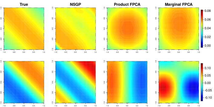
Figure 3: First two leading eigensurfaces $\phi_{j}(s_{1},s_{2})$ of the true (based on Chebyshev polynomials) model (first column) and the corresponding eigensurfaces $\hat{\phi}_{j}(s_{1},s_{2})$ estimated by NSGP model (with Matérn $\nu=1.5$) (second column), Product FPCA (third) and Marginal FPCA (fourth).

4.2   Simulation Study 2

The purpose of this simulation study is to assess the estimation accuracy of a given spatially-varying anisotropy matrix for different sample sizes. We simulate ten realizations from a function-valued process $X(s_{1},s_{2})$, where $s_{q}\in{\cal T}_{q}\subset\left[0,1\right],\ q=1,2$, from (1), where $f$ is zero-mean Gaussian process with covariance function (10), exponential correlation kernel $g(\cdot)$ and $\sigma(s_{1},s_{2})=1$. The elements of the true varying anisotropy matrix $\bm{{A}}(s_{1},s_{2})$ are:

$$\bm{{A}}_{11}(s_{1},s_{2})=\exp\big{(}6\cos(10s_{1}-5s_{2})\big{)},\qquad\bm{{A}}_{22}(s_{1},s_{2})=\exp\big{(}\sin(6s_{1}^{3})+\cos(6s_{2}^{4})\big{)},$$ (39)

$$\bm{{A}}_{12}(s_{1},s_{2})=\{\bm{{A}}_{11}(s_{1},s_{2})\bm{{A}}_{22}(s_{1},s_{2})\}^{1/2}\rho_{12}(s_{1},s_{2}),\quad\rho_{12}(s_{1},s_{2})=\tanh\big{(}(s_{1}^{2}+s_{2}^{2})/2\big{)}.$$ (40)

The unconstrained parameters associated to the varying anisotropy matrix are modeled via (38), using $L=M=6$ B-spline basis functions with evenly spaced knots. To assess the estimation accuracy of the elements of $\bm{{A}}(s_{1},s_{2})$, we employ the integrated squared error

$$\text{ISE}\Big{(}\log\hat{\bm{{A}}}_{pq}(s_{1},s_{2})\Big{)}=\int_{\mathcal{T}_{1}}\int_{\mathcal{T}_{2}}\left[\log\bm{{A}}_{pq}(s_{1},s_{2})-\log\hat{\bm{{A}}}_{pq}(s_{1},s_{2})\right]^{2}ds_{2}ds_{1}.$$ (41)

ISE results in Table 1 show that the estimates of $\bm{{A}}(s_{1},s_{2})$ are very good for fairly small sample sizes ($20\times 20$), and can be obtained without much computational time. The implementation was conducted on a 16GB, 2.20GHz Linux machine.

Nelson-Aalen plots (Figure 1(b)) show that the estimated model becomes more consistent with the true one as the sample size increases. Estimated eigensurfaces and corresponding CFVE can be seen in Section LABEL:sec:SupplSimConv of the Supplementary Material.

Table 1: ISE for the elements of the varying anisotropy matrix which was estimated by using different sample sizes $n$. The last column displays the estimation time.

$n$	$\log\hat{\bm{{A}}}_{11}(s_{1},s_{2})$	$\log\hat{\bm{{A}}}_{22}(s_{1},s_{2})$	$\hat{\rho}_{12}(s_{1},s_{2})$	time (hours)
100	68.9580	32.6482	0.9002	0.17
225	10.6267	12.4810	0.2883	0.42
400	1.2665	0.3339	0.2365	0.89
900	1.7725	0.1105	0.3265	2.54

5   Application to Wind Intensity Data

In this application, we aim to illustrate the benefits of using NSGP model and some comparison with separable, stationary models. In order to examine nonseparability aspects, as discussed previously, we look at data standardized by the standard deviation across realizations and then analyze the correlation structure. We interpret the empirical correlation function as the true one. We highlight, though, that the empirical correlation function is only available because there exist multiple realizations and that these are on the same grid.

The application is to annual wind intensities at $10$m in 2006. The dataset is used by Garside et al. (2020) and consists of $30$ realizations observed on a $51\times 96$ (latitude $\times$ longitude) grid. At each point in the grid, the data are standardized by the mean and standard deviation of the $30$ values at that location, so that we assume zero mean function and unit marginal variance. A realization is shown in Figure 5(a).

Figure 4 displays Nelson-Aalen results for the $30$ realizations and for a few competing models. The empirical correlation function seems to represent well the overall behavior of the $30$ realizations, and is interpreted as the Nelson-Aalen for the true correlation function.

We fit a Gaussian process regression model with four parametric separable, stationary correlation functions – Exponential, Matérn ($\nu=1.5$), Matérn ($\nu=2.5$) and Gaussian. We also fit NSGP model (10) with $\sigma(s_{1},s_{2})=1$ and with the same four specifications for the correlation function $g$. The unconstrained elements of the spatially-varying anisotropy matrix are modeled via (38), using $L=M=5$ B-spline basis functions with evenly spaced knots. Cyclic B-spline basis functions are used for the longitudinal direction.

Figure 4 suggests that the model based on the product of marginal covariance functions is not consistent with the data. With regards to Gaussian process-based models, for each correlation kernel the introduction of nonseparability and nonstationarity improves the results in terms of Nelson-Aalen estimates. For example, when Matérn ($\nu=1.5$) is used, the separable, stationary model overestimates the cumulative hazard function, while NSGP model based on the same correlation kernel seems to provide a much better fit.

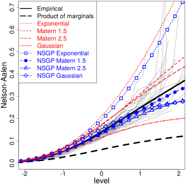
Figure 4: Nelson-Aalen plots for wind intensity data. Grey lines represent the results for the $30$ realizations. The continuous, thick line is based on the empirical correlation function. The dashed, thick line is on the product representation model. The other lines are results based on separable, stationary Gaussian process models and NSGP models with different specifications for $g$.

Figure 5 displays the elements of the varying anisotropy matrix estimated by NSGP model with Matérn ($\nu=1.5$) correlation function $g$. The estimates of both spatially varying decay parameters $\bm{{A}}_{11}(s_{1},s_{2})$ and $\bm{{A}}_{22}(s_{1},s_{2})$ are in general lower in oceanic regions, suggesting that the spatial process is smoother in these regions in both north-south and west-east directions. The estimate of the degree of nonseparability $\rho_{12}(s_{1},s_{2})$ is between $-0.765$ and $0.968$, indicating strong interaction between longitude and latitude in the covariance structure in some regions. Large positive values indicate that the spatial process changes more quickly towards north-eastward and south-westward directions. In the Southern Cone – the southernmost areas of South America – that is expected because of a typical wind (locally known as Minuano) that brings low temperature towards north-east. Similarly, large negative values (in the center of the figure) can be associated to the well-known winds coming from the west coast of Africa to the Caribbean Sea.

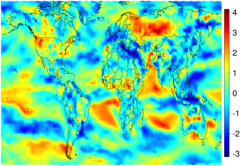
(a)

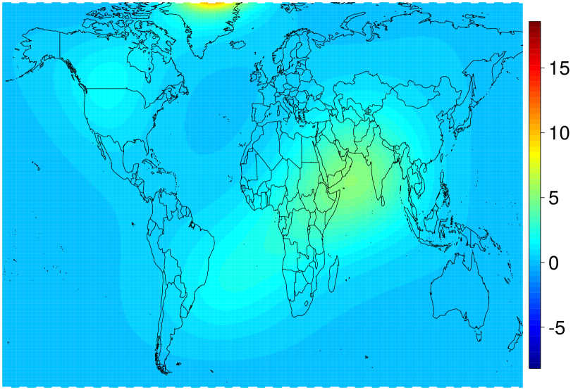
(b)

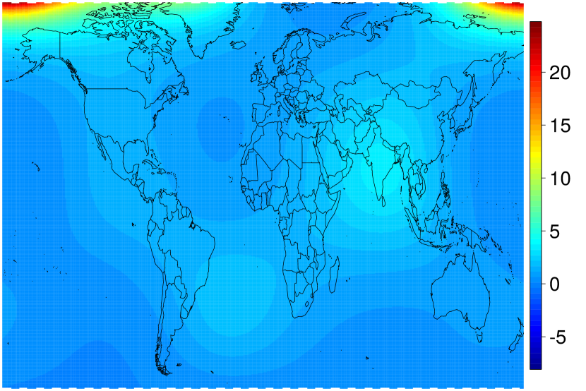
(c)

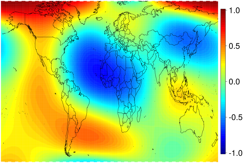
(d)

Figure 5: (a) One of the 30 realizations from the annual wind intensity data. (b), (c) and (d) show the elements of the varying anisotropy matrix obtained by NSGP model with Matérn ($\nu=1.5$) correlation function $g$: (b) $\bm{{A}}_{11}(s_{1},s_{2})$; (c) $\bm{{A}}_{22}(s_{1},s_{2})$; and (d) degree of nonseparability $\rho_{12}(s_{1},s_{2})$.

6   Discussion

Whereas nonparametric models for the covariance function are flexible but difficult to estimate in multidimensional domains due to the curse of dimensionality problem, parametric models can easily be estimated but their flexibility is limited by the choice of parametric covariance function, which is usually either stationary or separable. We proposed to use a flexible, convolution-based approach which allows for nonstationarity and nonseparability, crucial properties to achieve good fit of the covariance function, extract the most important modes of variation in the data and obtain better estimates of uncertainty in predictions. This approach is readily applied to multidimensional domains.

The unconstrained estimation of the parameters in the varying anisotropy matrix enables us to model them as a function of time or spatial location easily. They can be further modeled as a function of time (or spatially) dependent covariates or other covariates. In any of these cases, the function can be represented by a variety of basis functions, among which we have found B-splines basis very suitable for ensuring smoothness and being flexible. In particular, our proposed spherical parametrization for $\bm{{A}}_{Q\times Q}(\bm{{t}})$, which allows us to easily deal with input dimensions higher than two, is specified by a decomposition whose elements have statistical interpretation.

When estimating $\tau$-varying parameters using B-spline basis in (18), using all the data (rather than the local likelihood estimation (LLE)) may require a potentially high computational cost. However, when computational costs are not prohibitive, this approach should be preferable to the LLE approach, whose performance heavily depends on the neighborhood size $r$. In the LLE, if a small neighborhood is used (e.g., in order to model very local features), one might obtain unstable local estimates. On the other hand, if a large neighborhood is used (something necessary when data are sparse), then the local stationarity assumption may be no longer appropriate and local estimates might be very biased.

Instead of using empirical Bayes estimates, we could have defined a hyperprior distribution for $\bm{{\theta}}$. In this case, our knowledge (posterior distribution) about $\bm{{\theta}}$ is updated as more data are observed. Finding the mode of the posterior density is a way to find what we call the maximum a posteriori (MAP) estimate of $\bm{{\theta}}$. When we use a non-informative or a uniform prior distribution, the MAP estimates are precisely the same as the empirical Bayes estimates (Shi & Choi, 2011).

The decomposition of GPs may be important for developing efficient approximation for big data, non-Gaussian data (Wang & Shi, 2014) and heavy-tailed data (Shah et al., 2014; Wang et al., 2017; Cao et al., 2018). For non-Gaussian and heavy-tailed data, the decomposition might be used instead of their predictive distributions which are usually complicated. It can also be important for further analysis of scalar-on-functions or function-on-functions regression models, where we try to reduce the dimension of data by using a small number of components. Our proposed approach can be especially important when these components (eigensurfaces) are nonseparable, as we have seen in the simulation studies.

Convolution-based GP methods can also be used to deal with multivariate GP outputs. For example, dependence between spatial processes is discussed in Ver Hoef & Barry (1998) and used by Boyle & Frean (2004) to work with multiple outputs. Considering nonstationarity in the multivariate setting is a topic for future research.

SUPPLEMENTARY MATERIAL

Supplementary Material:

It contains proofs, technical derivations, additional numerical results, and an additional application to relative humidity data

References

- (1)
- Allen et al. (2014) Allen, G. I., Grosenick, L. & Taylor, J. (2014), ‘A generalized least-square matrix decomposition’, Journal of the American Statistical Association 109(505), 145–159.
- Aston et al. (2017) Aston, J. A., Pigoli, D., Tavakoli, S. et al. (2017), ‘Tests for separability in nonparametric covariance operators of random surfaces’, The Annals of Statistics 45(4), 1431–1461.
- Ba & Joseph (2012) Ba, S. & Joseph, V. R. (2012), ‘Composite Gaussian process models for emulating expensive functions’, Ann. Appl. Stat. 6(4), 1838–1860.
- Banerjee et al. (2015) Banerjee, S., Carlin, B. P. & Gelfand, A. E. (2015), Hierarchical modeling and analysis for spatial data, 2nd edn, CRC Press.
- Boyle & Frean (2004) Boyle, P. & Frean, M. (2004), Dependent Gaussian processes, in ‘Advances in neural information processing systems’, pp. 217–224.
- Bruno et al. (2009) Bruno, F., Guttorp, P., Sampson, P. D. & Cocchi, D. (2009), ‘A simple non-separable, non-stationary spatiotemporal model for ozone’, Environmental and ecological statistics 16(4), 515–529.
- Calandra et al. (2016) Calandra, R., Peters, J., Rasmussen, C. E. & Deisenroth, M. P. (2016), Manifold Gaussian processes for regression, in ‘Neural Networks (IJCNN), 2016 International Joint Conference on’, IEEE, pp. 3338–3345.
- Cao et al. (2018) Cao, C., Shi, J. Q. & Lee, Y. (2018), ‘Robust functional regression model for marginal mean and subject-specific inferences’, Statistical Methods in Medical Research 27(11), 3236–3254.
- Cappello et al. (2018) Cappello, C., De Iaco, S. & Posa, D. (2018), ‘Testing the type of non-separability and some classes of space-time covariance function models’, Stochastic Environmental Research and Risk Assessment 32(1), 17–35.
- Carlin & Louis (2008) Carlin, B. P. & Louis, T. A. (2008), Bayesian methods for data analysis, CRC Press.
- Chen et al. (2017) Chen, K., Delicado, P. & Müller, H.-G. (2017), ‘Modelling function-valued stochastic processes, with applications to fertility dynamics’, Journal of the Royal Statistical Society: Series B (Statistical Methodology) 79(1), 177–196.
- Chen & Müller (2012) Chen, K. & Müller, H.-G. (2012), ‘Modeling repeated functional observations’, Journal of the American Statistical Association 107(500), 1599–1609.
- Chen et al. (2019) Chen, Y., Carroll, C., Dai, X., Fan, J., Hadjipantelis, P. Z., Han, K., Ji, H., Mueller, H.-G. & Wang, J.-L. (2019), fdapace: Functional Data Analysis and Empirical Dynamics. R package version 0.5.1.
- Constantinou et al. (2017) Constantinou, P., Kokoszka, P. & Reimherr, M. (2017), ‘Testing separability of space-time functional processes’, Biometrika 104(2), 425–437.
- Cressie & Huang (1999) Cressie, N. & Huang, H.-C. (1999), ‘Classes of nonseparable, spatio-temporal stationary covariance functions’, Journal of the American Statistical Association 94(448), 1330–1339.
- de Boor (2001) de Boor, C. (2001), A Practical Guide to Splines, New York: Springer.
- De Iaco et al. (2002) De Iaco, S., Myers, D. E. & Posa, D. (2002), ‘Nonseparable space-time covariance models: some parametric families’, Mathematical Geology 34(1), 23–42.
- Deisenroth & Ng (2015) Deisenroth, M. & Ng, J. W. (2015), Distributed Gaussian Processes, in F. Bach & D. Blei, eds, ‘Proceedings of the 32nd International Conference on Machine Learning’, Vol. 37 of Proceedings of Machine Learning Research, PMLR, Lille, France, pp. 1481–1490.
- Dunlop et al. (2018) Dunlop, M. M., Girolami, M. A., Stuart, A. M. & Teckentrup, A. L. (2018), ‘How Deep Are Deep Gaussian Processes?’, Journal of Machine Learning Research 19(54), 1–46.
- Eddelbuettel & François (2011) Eddelbuettel, D. & François, R. (2011), ‘Rcpp: Seamless R and C++ integration’, Journal of Statistical Software 40(8), 1–18.
- Eddelbuettel & Sanderson (2014) Eddelbuettel, D. & Sanderson, C. (2014), ‘RcppArmadillo: Accelerating R with high-performance C++ linear algebra’, Computational Statistics and Data Analysis 71, 1054–1063.
- Garside et al. (2020) Garside, K., Henderson, R., Johnson, H. & Makarenko, I. (2020), Topological event history analysis, Technical report, Newcastle University, UK.
- Gneiting (2002) Gneiting, T. (2002), ‘Nonseparable, stationary covariance functions for space–time data’, Journal of the American Statistical Association 97(458), 590–600.
- Hall et al. (2008) Hall, P., Müller, H.-G., & Yao, F. (2008), ‘Modelling sparse generalized longitudinal observations with latent gaussian processes’, Journal of the Royal Statistical Society. Series B (Methodological) 70.
- Higdon (1998) Higdon, D. (1998), ‘A process-convolution approach to modelling temperatures in the North Atlantic Ocean’, Environmental and Ecological Statistics 5(2), 173–190.
- Higdon (2002) Higdon, D. (2002), Space and space-time modeling using process convolutions, in ‘Quantitative methods for current environmental issues’, Springer, pp. 37–56.
- Higdon et al. (1999) Higdon, D., Swall, J. & Kern, J. (1999), ‘Non-stationary spatial modeling’, Bayesian statistics 6(1), 761–768.
- Jidling et al. (2017) Jidling, C., Wahlström, N., Wills, A. & Schön, T. B. (2017), Linearly constrained gaussian processes, in ‘Advances in Neural Information Processing Systems’, pp. 1215–1224.
- Jun & Stein (2007) Jun, M. & Stein, M. L. (2007), ‘An approach to producing space: Time covariance functions on spheres’, Technometrics 49(4), 468–479.
- Jun & Stein (2008) Jun, M. & Stein, M. L. (2008), ‘Nonstationary covariance models for global data’, The Annals of Applied Statistics 2(4), 1271–1289.
- Kanagawa et al. (2018) Kanagawa, M., Hennig, P., Sejdinovic, D. & Sriperumbudur, B. K. (2018), ‘Gaussian processes and kernel methods: A review on connections and equivalences’, Preprint, ArXiv:1807.02582 .
- Leng et al. (2010) Leng, C., Zhang, W. & Pan, J. (2010), ‘Semiparametric mean–covariance regression analysis for longitudinal data’, Journal of the American Statistical Association 105(489), 181–193.
- Liu et al. (2018) Liu, H., Cai, J., Ong, Y.-S. & Wang, Y. (2018), ‘Understanding and Comparing Scalable Gaussian Process Regression for Big Data’, Preprint, ArXiv:1811.01159 .
- O’Hagan (1978) O’Hagan, A. (1978), ‘Curve fitting and optimal design for prediction’, Journal of the Royal Statistical Society. Series B (Methodological) 40(1), 1–42.