Fast Compressed Power Spectrum Estimation: Towards A Practical Solution for Wideband Spectrum Sensing

Abstract

There has been a growing interest in wideband spectrum sensing due to its applications in cognitive radios and electronic surveillance. To overcome the sampling rate bottleneck for wideband spectrum sensing, in this paper, we study the problem of compressed power spectrum estimation whose objective is to reconstruct the power spectrum of a wide-sense stationary signal based on sub-Nyquist samples. By exploring the sampling structure inherent in the multicoset sampling scheme, we develop a computationally efficient method for power spectrum reconstruction. An important advantage of our proposed method over existing compressed power spectrum estimation methods is that our proposed method, whose primary computational task consists of fast Fourier transform (FFT), has a very low computational complexity. Such a merit makes it possible to efficiently implement the proposed algorithm in a practical field-programmable gate array (FPGA)-based system for real-time wideband spectrum sensing. Our proposed method also provides a new perspective on the power spectrum recovery condition, which leads to a result similar to what was reported in prior works. Simulation results are presented to show the computational efficiency and the effectiveness of the proposed method.

I Introduction

The scarcity of spectrum resource is a critical problem for future wireless communications and Internet of Things [1]. Dynamic spectrum access [2] allows the idle spectrum to be used by unlicensed users and provides a promising way to enhance the spectrum efficiency. Real-time spectrum sensing, which empowers the secondary user to identify spectrum holes, is a fundamental technique to dynamic spectrum sensing and has received much interest over the past decade [3, 4]. However, most previous studies, e.g. [3, 4, 5], focus on narrowband spectrum sensing. Only a few touched the topic of wideband spectrum sensing until recently, e.g. [6]. As the cognitive radio networks are expected to operate over a wide frequency range, wideband spectrum sensing is important for future cognitive radio systems. In addition, in some applications such as electronic surveillance, one also needs to perform wideband spectrum sensing to identify the frequency locations of a number of signals that spread over a wide frequency band. A conventional receiver requires to sample the received signal at the Nyquist rate, which may be too power hungry due to the use of high speed analog-digital converters (ADCs) or even infeasible if the spectrum under monitoring is very wide, say, of several GHz. One way to overcome this difficulty is to divide the frequency spectrum under monitoring into a number of separate frequency segments and then sequentially scan these frequency channels. Nevertheless, such a scanning scheme incurs a sensing latency and may fail to capture short-lived signals [7].

The recently emerged technique compressed sensing [8] provides a new approach to sensing a wide frequency band via low sampling rate ADCs. Motivated by the fact that the spectrum in general is severely underutilized in a specific geographic area, the rationale behind such schemes is to exploit the inherent sparsity in the frequency domain and formulate wideband spectrum sensing as a sparse signal recovery problem which, according to the compressed sensing theory [9, 8], can perfectly recover the signal of the entire frequency band based on sub-Nyquist samples. Different compressed sampling architectures and sparse signal recovery algorithms, e.g. [10, 11, 12, 13, 14, 15, 16], were developed for wideband spectrum sensing over the past few years. Such an approach, however, suffers several drawbacks. Firstly, reconstructing the original signal of the entire frequency band via sparse signal recovery methods involves a prohibitively high computational complexity for practical systems. Secondly, due to the noise across a wide frequency band, the receiver usually has a low signal-to-noise ratio. While in the low signal-to-noise ratio regime, sparse signal recovery methods yield barely satisfactory recovery performance.

To overcome these difficulties, some works proposed to reconstruct the power spectrum of the wideband signal, instead of the original signal itself, from sub-Nyquist samples [17, 18, 19, 20, 21, 22]. Compared with recovering the original signal, reconstructing the power spectrum can significantly reduce the amount of data being stored and transmitted. Also, the use of statistical information enables the proposed algorithm to accurately perform spectrum sensing even in low signal-to-noise ratio environments. In addition, it was shown that it is even possible to perfectly reconstruct the power spectrum without placing any sparse constraint on the wideband spectrum under monitoring [18, 19, 20]. Overall, this approach seems to be a more practical solution for wideband spectrum sensing. Nevertheless, existing compressed power spectrum estimation methods still incur a high computational complexity that is impractical for real-time wideband spectrum sensing. To address this difficulty, notice that the data samples obtained via the multicoset sampling scheme are a subset of the Nyquist samples. Such a property allows us to establish an amiable relationship between the autocorrelation sequence and the sub-Nyquist samples, based on which we develop a computationally efficient algorithm for compressed power spectrum estimation. The proposed algorithm has a low computational complexity which scales linearly with the number of samples (in time) $L$ and the downsampling factor $N$. In contrast, existing compressed power spectrum estimation methods have a complexity either scaling polynomially with $L$ or scaling quadratically with $N$. Also, our proposed method, which involves the discrete Fourier transform (DFT) as its computationally dominant task, can be efficiently implemented via FFT algorithms. These advantages make it a practical solution for real-time wideband spectrum sensing.

The rest of the paper is organized as follows. In Section II, we provide a brief review of existing compressed wideband power spectrum estimation methods. In Section III, a computationally-efficient compressed power spectrum estimation algorithm is proposed, along with an analysis of the recovery condition and its computational complexity. Simulation results are presented in Section IV, followed by concluding remarks in Section V.

II Review of State-of-The-Arts

In this section, we provide a brief review of existing compressive wideband power spectrum estimation methods. Generally, the methods, according to the way of formulation, can be divided into a time-domain approach and a frequency-domain approach.

Figure 1: Compressed sampling architecture: analog to information converter (AIC)

II-A Time-Domain Power Spectrum Reconstruction Approach

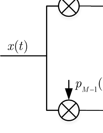
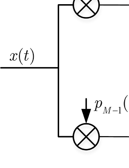
The time-domain approach reconstructs the power spectrum of a wide-sense stationary multi-band signal $x(t)$ by exploring a relationship between the autocorrelation of the Nyquist samples and the autocorrelation of the sub-Nyquist samples. Here the sub-Nyquist samples are obtained via a compressed sampling scheme such as the analog to information converter (AIC) [23] or the multicoset sampling scheme [24]. Let us take the AIC for an example. The AIC (see Fig. 1) consists of a number of sampling channels, also referred to as branches. In each branch, say branch $m$, the signal $x(t)$ is modulated by a periodic pseudo-noise (PN) sequence $p_{m}(t)$ of period $NT$, and then passes through an integrate-and-dump device with period $NT$. Here $T$ denotes the Nyquist sampling interval. $N$, a positive integer, is the downsampling factor of user’s choice, i.e. the sampling rate at each branch is equal to $1/N$ times the Nyquist rate. Assume that the PN sequence is a piecewise constant signal with constant values in every interval of length $T$, i.e.

$$p_{m}(t)=c_{m}[n]\quad nT\leq t<(n+1)T.$$ (1)

The output of the $m$th branch at the $l$th sampling instant can be expressed as

$$y_{m}[l]=\boldsymbol{c}^{T}_{m}\boldsymbol{x}[l],$$ (2)

where

$$\boldsymbol{c}_{m}\triangleq[c_{m}[0]\phantom{0}c_{m}[1]\phantom{0}\ldots\phantom{0}c_{m}[N-1]]^{T},$$ (3)

and

$$\boldsymbol{x}[l]\triangleq[x[lN]\phantom{0}x[lN+1]\phantom{0}\ldots\phantom{0}x[(l+1)N-1]]^{T},$$ (4)

in which $x[lN+n]$ is the average level of $x(t)$ at time interval $[lNT+nT,lNT+(n+1)T]$.

Let $\boldsymbol{y}[l]\triangleq[y_{1}[l]\phantom{0}\dots\phantom{0}y_{M}[l]]^{T}$ denote the data sample vector collected at the $l$th sampling time instant. We have

$$\boldsymbol{y}[l]=\boldsymbol{C}\boldsymbol{x}[l],$$ (5)

where $\boldsymbol{C}\triangleq[\boldsymbol{c}_{1}\phantom{0}\ldots\phantom{0}\boldsymbol{c}_{M}]^{T}$. Calculating the autocorrelation of $\boldsymbol{y}[l]$ yields:

$$\boldsymbol{R}_{y}\triangleq \mathbb{E}[\boldsymbol{y}[l]\boldsymbol{y}^{H}[l]]=\boldsymbol{C}\mathbb{E}[\boldsymbol{x}[l]\boldsymbol{x}^{H}[l]]\boldsymbol{C}^{H}$$

$$= \boldsymbol{C}\boldsymbol{R}_{x}\boldsymbol{C}^{H},$$ (6)

where $\boldsymbol{R}_{x}\triangleq\mathbb{E}[\boldsymbol{x}[l]\boldsymbol{x}^{H}[l]]$. Note that here $\boldsymbol{x}[l]$ can be considered as a vector constructed by $N$ consecutive Nyquist samples. Hence (6) establishes the relationship between the autocorrelation of the Nyquist samples and the autocorrelation of the sub-Nyquist samples. We see that $\boldsymbol{R}_{x}$ is a Toeplitz matrix, with its $(n+m,n)$th entry equal to $r_{x}[m]\triangleq E[x[n+m]x^{\ast}[n]]$. Moreover, as $x(t)$ is a real-valued signal, we have $r_{x}[m]=r_{x}[-m]$. Define

$$\boldsymbol{r}_{x}\triangleq[r_{x}[0]\phantom{0}r_{x}[1]\phantom{0}\dots\phantom{0}r_{x}[N-1]]^{T}.$$ (7)

Clearly, we can express the vectorized form of $\boldsymbol{R}_{x}$ as: $\text{vec}(\boldsymbol{R}_{x})=\boldsymbol{B}\boldsymbol{r}_{x}$, where $\text{vec}(\cdot)$ denotes the vectorization operation, $\boldsymbol{B}\in\{0,1\}^{N^{2}\times N}$ is the corresponding selection matrix. Taking the vectorization of $\boldsymbol{R}_{y}$, we obtain

$$\text{vec}(\boldsymbol{R}_{y})=(\boldsymbol{C}^{*}\otimes\boldsymbol{C})\boldsymbol{B}\boldsymbol{r}_{x}\triangleq\boldsymbol{\Phi}\boldsymbol{r}_{x},$$ (8)

where $\otimes$ denotes the Kronecker product, and $\boldsymbol{\Phi}\triangleq(\boldsymbol{C}^{*}\otimes\boldsymbol{C})\boldsymbol{B}$ is an $M^{2}\times N$ matrix. Since $\boldsymbol{B}$ is full column rank, we can let $M^{2}>N$ and carefully select the PN sequences such that $\boldsymbol{\Phi}$ is a full column rank matrix. Thus $\boldsymbol{r}_{x}$ can be easily calculated as

$$\boldsymbol{r}_{x}=\boldsymbol{\Phi}^{{\dagger}}\text{vec}(\boldsymbol{R}_{y}),$$ (9)

and the power spectrum of the original signal $x(t)$ can be reconstructed by taking the discrete Fourier transform (DFT) of $\boldsymbol{r}_{x}$.

It should be noted that the resolution of the recovered power spectrum is determined by the length of the autocorrelation sequence $\boldsymbol{r}_{x}$, i.e. $N$. On the other hand, we require $M^{2}>N$ to make $\boldsymbol{\Phi}$ invertible and $M$, the number of sampling branches, cannot be arbitrarily large due to hardware complexity and cost. As a result, $N$ cannot be chosen to be very large, which prevents us from obtaining a high-resolution power spectrum. To address this issue, one can collect multiple samples $\boldsymbol{y}[l],l=0,\ldots,L-1$ and stack them into a long vector $\boldsymbol{y}$. Specifically, define

$$\boldsymbol{x}\triangleq [\boldsymbol{x}^{T}[0]\phantom{0}\dots\phantom{0}\boldsymbol{x}^{T}[L-1]]^{T},$$

$$\boldsymbol{y}\triangleq [\boldsymbol{y}^{T}[0]\phantom{0}\dots\phantom{0}\boldsymbol{y}^{T}[L-1]]^{T}.$$

Then we have

$$\boldsymbol{y}=(\boldsymbol{I}_{L}\otimes\boldsymbol{C})\boldsymbol{x}\triangleq\boldsymbol{\bar{C}}\boldsymbol{x},$$ (10)

where $\boldsymbol{I}_{L}$ denotes an $L\times L$ identity matrix. Calculating the autocorrelation of $\boldsymbol{y}$ yields:

$$\boldsymbol{\bar{R}}_{y}=\boldsymbol{\bar{C}}\boldsymbol{\bar{R}}_{x}\boldsymbol{\bar{C}}^{H}.$$ (11)

Similarly, the autocorrelation sequence $\boldsymbol{\bar{r}}_{x}\triangleq[r_{x}[0]\phantom{0}\dots\phantom{0}r_{x}[LN-1]]^{T}$ can be estimated as

$$\boldsymbol{\bar{r}}_{x}=((\boldsymbol{\bar{C}}^{*}\otimes\boldsymbol{\bar{C}})\boldsymbol{\bar{B}})^{{\dagger}}\text{vec}(\boldsymbol{\bar{R}}_{y}),$$ (12)

where $\boldsymbol{\bar{B}}\in\{0,1\}^{(LN)^{2}\times LN}$ is the corresponding selection matrix. Note that the autocorrelation sequence $\boldsymbol{\bar{r}}_{x}$ has a dimension of $NL$, from which we can obtain a power spectrum of length $(2NL-1)$ with a spectrum resolution $1/((2NL-1)T)$. Thus a desired high-resolution power spectrum can be achieved by choosing a proper value of $L$.

In summary, the time-domain approach consists of three steps, namely, calculating the correlation matrix $\boldsymbol{\bar{R}}_{y}$, estimating $\boldsymbol{\bar{r}}_{x}$ via (12), and reconstructing the power spectrum by taking the Fourier transform of $\boldsymbol{\bar{r}}_{x}$. The correlation matrix $\boldsymbol{\bar{R}}_{y}$ can be estimated as

$$\boldsymbol{\hat{\bar{R}}}_{y}=\frac{1}{P}\sum_{p=1}^{P}\boldsymbol{y}_{p}\boldsymbol{y}^{H}_{p},$$ (13)

where

$$\boldsymbol{y}_{p}\triangleq [\boldsymbol{y}^{T}[p]\phantom{0}\dots\phantom{0}\boldsymbol{y}^{T}[L+p-1]]^{T}.$$ (14)

The matrix $((\boldsymbol{\bar{C}}^{*}\otimes\boldsymbol{\bar{C}})\boldsymbol{\bar{B}})^{{\dagger}}$ in (12) can be computed in advance. Thus we only need to perform a matrix-vector product to obtain $\bar{\boldsymbol{r}}_{x}$. We can easily verify that these three steps involve $PL^{2}M^{2}$, $L^{3}M^{2}N$, and $(2LN-1)\log(2LN-1)$ floating-point operations, respectively, which scale polynomially with the number of samples, $L$, making the time-domain approach infeasible for practical systems. To see this, suppose we would like to sense a wide frequency band up to 1GHz. Set $M=8$ and $N=25$. In order to obtain a spectrum resolution of 10kHz, we need to set $L=4000$, in which case the total number of floating-point operations is at least as large as $2.5\times 10^{13}$, and it will take a few hours to complete the computational task even with a high-performance FPGA. We note that a more efficient time-domain approach was developed in [18], which has a computational complexity similar to the frequency-domain approach analyzed below.

Figure 2: Compressed sampling architecture: modulated wideband converter (MWC)

II-B Frequency-Domain Power Spectrum Reconstruction Approach

In addition to the time-domain approach, another approach deals with the power spectrum estimation problem from a frequency viewpoint. The frequency-domain approach was originally proposed in [20], in which the sub-Nyquist data samples are obtained via a compressed sampling scheme termed as modulated wideband converter (MWC) [25]. The MWC has an architecture similar to the AIC, but replaces the integrate devices with low-pass filters. Different from the time-domain approach, the frequency-domain approach aims to establish the relationship between the frequency representation of the original signal and the frequency representation of the compressed samples.

Note that the PN sequence is periodic with a period $NT$. It, therefore, has a discrete spectrum consisting of an infinite number of impulses. According to the convolution properties, the spectrum of the PN sequence-modulated signal in each branch is a weighted combination of the spectrum of the original signal $x(t)$ and its frequency-shifted versions. By setting the cutoff frequency of the low-pass filters to $1/(2NT)$, the spectrum of the low-pass filtered signal at each branch is a superposition of $N$ segments. Here the $N$ segments are obtained via dividing the spectrum of the original signal $x(t)$ into $N$ segments of equal width. Mathematically, the relationship between the spectrum of the low-pass filtered signal and that of the original signal is given as [20]

$$\boldsymbol{y}(f)=\boldsymbol{A}\boldsymbol{x}(f),$$ (15)

where the $m$th entry of $\boldsymbol{y}(f)$ denotes the Fourier transform of the filtered signal at the $m$th branch, $\boldsymbol{A}$ denotes the mixture matrix determined by the spectrum of the PN sequences, and the $n$th element of $\boldsymbol{x}(f)$, denoted by $x_{n}(f)$, is the $n$th segment of the spectrum of the original signal, which is given as

$$x_{n}(f)=\begin{cases}X(f+\frac{2n-N-1}{2NT})&\text{if $N$ is odd}\\ X(f+\frac{2n-N-2}{2NT})&\text{if $N$ is even}\end{cases},$$ (16)

$\forall f\in(-\frac{1}{2NT},\frac{1}{2NT}]$, where $X(f)$ denotes the frequency spectrum of the original signal $x(t)$.

Calculating the correlation of $\boldsymbol{y}(f)$ gives

$$\boldsymbol{R}_{y}(f)= \mathbb{E}[\boldsymbol{y}(f)\boldsymbol{y}^{H}(f)]=\boldsymbol{A}\mathbb{E}[\boldsymbol{x}(f)\boldsymbol{x}^{H}(f)]\boldsymbol{A}^{H}$$

$$\triangleq \boldsymbol{A}\boldsymbol{R}_{x}(f)\boldsymbol{A}^{H}.$$ (17)

For a wide-sense stationary signal $x(t)$, its Fourier transform $X(f)$ has the following property

$$\mathbb{E}[X(f_{1})X^{*}(f_{2})]=\begin{cases}0,&f_{1}\neq f_{2}\\ P(f_{1}),&f_{1}=f_{2}\end{cases},$$ (18)

where $P(f)$ is the power spectrum of $x(t)$. Thus $\boldsymbol{R}_{x}(f)$ is a diagonal matrix and (17) can be rewritten as

$$\text{vec}(\boldsymbol{R}_{y}(f))=(\boldsymbol{A}^{*}\odot\boldsymbol{A})\boldsymbol{r}_{x}(f),$$ (19)

where $\odot$ denotes the Khatri-Rao product, and $\boldsymbol{r}_{x}(f)$ is a vector containing the diagonal entries of $\boldsymbol{R}_{x}(f)$. It is easy to see that if $\boldsymbol{A}^{*}\odot\boldsymbol{A}$ has a full column rank, then $\boldsymbol{r}_{x}(f)$ can be estimated from $\boldsymbol{R}_{y}(f)$, i.e.

$$\boldsymbol{r}_{x}(f)=(\boldsymbol{A}^{*}\odot\boldsymbol{A})^{{\dagger}}\text{vec}(\boldsymbol{R}_{y}(f)).$$ (20)

One can carefully design the PN sequences such that if $M^{2}\geq N$, the matrix $\boldsymbol{A}^{*}\odot\boldsymbol{A}$ has a full column rank. Note that the $n$th entry of $\boldsymbol{r}_{x}(f)$ is given as $r_{x,n}(f)=\mathbb{E}[x_{n}(f)x^{*}_{n}(f)]$. We uniformly discretize the frequency range $(-1/(2NT),1/(2NT)]$ into $2L$ grid points, say $f_{1},f_{2},\ldots,f_{2L}$ and estimate $\boldsymbol{r}_{x}(f_{l}),\forall l\in\{1,\ldots,2L\}$ from (19). Accordingly, the power spectrum of the original signal can be reconstructed based on $\{\boldsymbol{r}_{x}(f_{l})\}$. Specifically, the reconstructed power spectrum vector has a dimension of $2NL$, with its $((n-1)L+1)$th entry equal to the $n$th element of $\boldsymbol{r}_{x}(f_{l})$. Clearly, the recovered power spectrum has a resolution of $1/(2NLT)$. More details about the frequency-domain approach can be found in [20].

We see that the frequency-domain method involves computing $\boldsymbol{y}(f)$, $\boldsymbol{R}_{y}(f)$, and (20). To compute $\boldsymbol{y}(f)$, we need to perform $2L$-point DFT of the time-domain signal for each channel, which needs $2LM\log(2L)$ floating-point operations. For a specific frequency $f_{l}$, $\boldsymbol{R}_{y}(f_{l})$ can be estimated as $\frac{1}{P}\sum_{p=1}^{P}\boldsymbol{y}_{p}(f_{l})\boldsymbol{y}_{p}(f_{l})^{H}$, where $\boldsymbol{y}_{p}(f_{l})\in\mathbb{C}^{M\times 1}$ is a sample vector obtained according to (15). It can be verified that calculating $\boldsymbol{R}_{y}(f_{l}),\forall l=\{1,\dots,2L\}$ needs $2M^{2}PL$ floating-point operations. Note that the pseudo-inverse of $(\boldsymbol{A}^{*}\odot\boldsymbol{A})$ can be computed off-line. Thus we only need to perform a matrix-vector product to compute $\boldsymbol{r}_{x}(f_{l})$ according to (20), which requires $M^{2}N$ floating-point operations. Consequently, calculating $\boldsymbol{r}_{x}(f_{l}),\forall l=\{1,\dots,2L\}$ needs $2M^{2}NL$ floating-point operations. Overall, to obtain a spectrum resolution of $1/(2NLT)$, the frequency-domain approach involves $2MLP\log(2L)+2M^{2}(N+P)L$ floating-point operations in total. Since we usually have $M\ll L$, the frequency-domain approach has a much lower computational complexity compared with the time-domain method. Note that we need $M^{2}\geq N$ to ensure that (19) is invertible. Hence we have $2M^{2}(N+P)L>2N^{2}L$, which implies that the computational complexity of the frequency-domain approach scales polynomially with the downsampling factor $N$. This makes it unsuitable for the high compression ratio scenario.

Figure 3: Compressed sampling architecture: multicoset sampling scheme

III Proposed Fast Compressed Power Spectrum Estimation Method

As discussed in our previous section, current compressed power spectrum estimation methods, particularly the time-domain approach, have a computational complexity that might be too excessive for real-time spectrum sensing systems. To address this issue, in this section, we develop a computationally efficient compressed power spectrum estimation method. In our proposed method, a multicoset sampling scheme is employed to collect sub-Nyquist data samples.

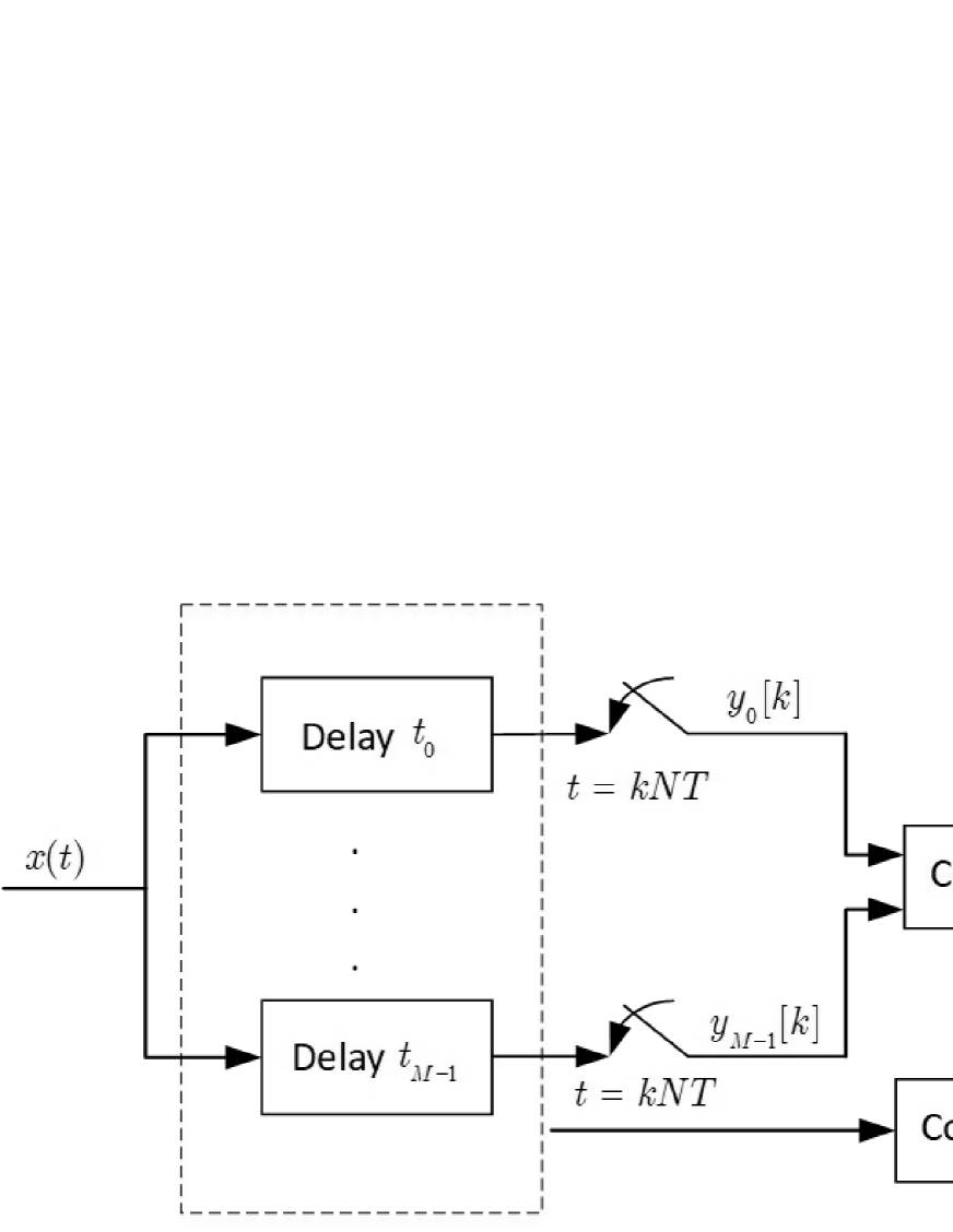
Before proceeding, we first introduce the multicoset sampling scheme. Similar to the AIC and the MWC, the multicoset sampling architecture consists of a number of sampling channels, also referred to as branches (see Fig. 3). In the $m$th branch, the analog signal $x(t)$ is delayed by an amount of time, $\Delta_{m}T$, and then sampled by a synchronized low-rate ADC whose sampling interval is set to $NT$, where $T$ is the Nyquist sampling interval, and $\Delta_{m}$ is set to be an integer smaller than the downsampling factor $N$. Clearly, for the multicoset sampling scheme, the output of the $m$th branch at the $l$th sampling instant can be written as

$$y_{m}[l]=x(lNT+\Delta_{m}T)=x[lN+\Delta_{m}],$$ (21)

where $x[n]=x(nT)$ denotes the Nyquist sample of $x(t)$. Define $\boldsymbol{x}[l]\triangleq[x[lN]\phantom{0}\dots\phantom{0}x[(l+1)N-1]]^{T}$, and $\boldsymbol{y}[l]\triangleq[y_{1}[l]\phantom{0}\dots\phantom{0}y_{M}[l]]^{T}$. Then the data sample collected at the $l$th sampling time instant is given by

$$\boldsymbol{y}[l]=\boldsymbol{C}\boldsymbol{x}[l],$$ (22)

where $\boldsymbol{C}\in\{0,1\}^{M\times N}$ is a selection matrix with only one nonzero entry in each row. We see that (22) is similar to (5), except that $\boldsymbol{C}$ is defined in a different way. We can follow the approach discussed in Section II to reconstruct the power spectrum of the analog signal $x(t)$. But such an approach has a prohibitively high computational complexity. Notice that the data samples obtained via the multicoset sampling scheme are a subset of the Nyquist samples. As will be shown later, this property allows us to establish an amiable relationship between the autocorrelation sequence and the sub-Nyquist samples, based on which a fast compressed power spectrum estimation method can be developed. This is the reason why we use the multicoset sampler to collect sub-Nyquist samples for our proposed method.

We see that the data samples $\{y_{m}[l]\}_{m=1,l=0}^{M,L-1}$ obtained via the multicoset sampling scheme are a subset of the Nyquist samples $\{x[n]\}_{n=0}^{LN-1}$. To establish the connection between the sub-Nyquist samples and Nyquist samples, we define a data sequence $\{h[n]\}_{n=0}^{LN-1}$ and an indicator sequence $\{I[n]\}_{n=0}^{LN-1}$, respectively, as follows

$$h[n]=\begin{cases}y_{m}[l],&n=lN+\Delta_{m}\\ 0,&\text{otherwise}\end{cases},$$ (23)

and

$$I[n]=\begin{cases}1,&n=lN+\Delta_{m}\\ 0,&\text{otherwise}\end{cases}.$$ (24)

It is easy to verify that

$$h[n]=x[n]I[n].$$ (25)

We now show how to use the sequences $\{h[n]\}$ and $\{I[n]\}$ to estimate the power spectrum of $\{x[n]\}$. A widely-used unbiased estimate of the autocorrelation $r_{x}[k]=\mathbb{E}[x[n]x^{*}[n-k]]$ is given as

$$r_{x}[k]\approx\frac{1}{|\mathbb{Q}_{k}|}\sum_{n\in\mathbb{Q}_{k}}(x[n]x^{*}[n-k])\quad k\in[-LN+1,LN-1],$$ (26)

where $\mathbb{Q}_{k}\triangleq\{n|0\leq n-k\leq LN-1,0\leq n\leq LN-1\}$, and $|\mathbb{Q}_{k}|$ denotes the size of $\mathbb{Q}_{k}$. Since we only have access to $\{h[n]\}$, we propose a new unbiased estimate of $\{r_{x}[k]\}$ which is given as

$$r_{x}[k]\approx \frac{1}{Q_{k}}\sum_{n\in\mathbb{\hat{Q}}_{k}}(x[n]x^{*}[n-k])$$

$$= \frac{1}{Q_{k}}\sum_{n\in\mathbb{Q}_{k}}(h[n]h^{*}[n-k]),$$ (27)

where $\mathbb{\hat{Q}}_{k}\triangleq\{n|I[n]I[n-k]=1\}$ and $Q_{k}\triangleq|\mathbb{\hat{Q}}_{k}|$. The proposed estimator, which directly uses the sub-Nyquist samples, is quite simple and easy to understand. Once the autocorrelation sequence $\{r_{x}[k]\}$ is obtained, its power spectrum can readily be given as the Fourier transform of the autocorrelation sequence.

III-A Recovery Condition

Note that to estimate the power spectrum via (27), we have to make sure that $Q_{k}>0,\forall k\in[-LN+1,LN-1]$, i.e. for each $k\in[-LN+1,LN-1]$, the set $\mathbb{\hat{Q}}_{k}=\{n|I[n]I[n-k]=1\}$ is a non-empty set. To ensure this condition is satisfied, the time delays of the multicoset sampling scheme have to be carefully devised. We have the following result regarding the choice of the time delays $\{\Delta_{m}\}$.

Lemma 1

For any integer $n$ satisfying $|n|\leq\lfloor\frac{N}{2}\rfloor$, where $\lfloor x\rfloor$ is the floor function that outputs the greatest integer less than or equal to $x$, if there exist $m_{1},m_{2}\in\{1,\ldots,M\}$ and $c\in\{-1,0,1\}$ such that

$$n=\Delta_{m_{1}}-\Delta_{m_{2}}+cN,$$ (28)

then we have $Q_{k}>0$ for all $k\in[-LN+1,LN-1]$.

Proof:

See Appendix A. ∎

Remarks: We note that the recovery condition (28) is slightly relaxed than the sparse ruler condition given in [18], and is equivalent to the recovery condition given in [26] which is termed as the circular sparse ruler. For the sparse ruler condition [18], it requires the set $\{0,1,\dots,\lfloor N/2\rfloor\}$ to be a subset of $\{|\Delta_{m_{1}}-\Delta_{m_{2}}|:0<m_{1}\leq M,0<m_{2}\leq M\}$. Such a condition amounts to saying that for any integer $|n|\leq\lfloor N/2\rfloor$, their exist $m_{1}$ and $m_{2}$ such that

$$n=\Delta_{m_{1}}-\Delta_{m_{2}}.$$ (29)

We see that the condition (29) is the same as (28) if we set $c=0$. This means our condition (28) is more relaxed than the condition discussed in [18]. For example, let $N=8$, $M=4$. Then we have two different delay sets $\{\Delta_{m}\}=\{0,2,3,4\}$ and $\{\Delta_{m}\}=\{0,3,5,7\}$, both of which satisfy our condition (28). Nevertheless, only the first delay set satisfies (29). Finding a smallest number of branches, $M$, such that (28) can be met is referred to as the circular sparse ruler problem and has been investigated in previous studies, e.g. [27, 28]. Specifically, in [19], it was shown that if $M\geq(N+1)/2$, then one can always find a multicoset sampling pattern satisfying (29), and consequently (28). Furthermore, [27, 28] proposed some special universal sampling patterns for the scenario where $M<(N+1)/2$. Note that the condition (28) guarantees the recovery of the power spectrum, without placing any sparsity constraint on the spectrum under monitoring. In contrast, the earlier work [29] discussed a universal sampling pattern that ensures perfect recovery of a multi-band signal with a given spectral occupancy bound.

III-B Proposed Algorithm

Note that directly calculating $\{r_{x}[k]\}_{k=-LN+1}^{LN-1}$ via (27) will need a total number of $2L^{2}N^{2}+LN$ floating-point operations. Such a computational complexity would become unacceptable when $L$ is large, which is usually the case in order to provide a fine spectrum resolution. We now show how to use FFT to reduce the computational complexity of the proposed estimator (27). Define

$$r_{h}[k]=\sum_{n\in\mathbb{Q}_{k}}(h[n]h^{*}[n-k]),$$ (30)

where $\mathbb{Q}_{k}=\{n|0\leq n-k\leq LN-1,0\leq n\leq LN-1\}$. The above equation can be rewritten as

$$r_{h}[k]=\sum_{n=0}^{LN-1}(h[n]h^{*}[n-k]),$$ (31)

by setting $h[n]=0$ for $n<0$ and $n\geq LN$. We define a new sequence $\{\bar{h}[n]\}_{n=-LN+1}^{LN-1}$ as

$$\bar{h}[n]=\begin{cases}h[n],&LN-1\geq n\geq 0\\ 0,&-LN+1\leq n<0\end{cases},$$ (32)

and let $\{\hat{h}[n]\}_{n=-LN+1}^{LN-1}$ be the reverse of $\{\bar{h}[n]\}_{n=-LN+1}^{LN-1}$, i.e

$$\hat{h}[n]=\bar{h}[-n].$$ (33)

Then we have

$$r_{h}[k] =\begin{cases}\sum_{n=-LN+1+k}^{LN-1}(\bar{h}[n]\hat{h}^{*}[k-n]),&k\geq 0\\ \sum_{n=-LN+1}^{LN-1+k}(\bar{h}[n]\hat{h}^{*}[k-n]),&k<0\\ \end{cases}$$

$$\stackrel{{\scriptstyle(a)}}{{=}}\sum_{n=-LN-1}^{LN-1}(\bar{h}[n]\hat{h}_{P}^{*}[k-n])$$

$$=(\bar{h}\star\hat{h}^{*})[k],$$ (34)

where $P\triangleq 2NL-1$, $\hat{h}_{P}[n]$ is a periodic summation of $\hat{h}[n]$ defined as

$$\hat{h}_{P}[n]\triangleq\sum_{k=-\infty}^{+\infty}\hat{h}[n-kP],$$ (35)

$(a)$ comes from the fact that $\bar{h}[n]=0$ for $-LN+1\leq n<0$ and $\hat{h}_{P}[n]=\hat{h}[n-NL]=0$ for $-2NL+1<n\leq-NL$, and the symbol $\star$ in the last equality denotes the circular convolution.

Define

$$\boldsymbol{r}_{h} \triangleq[r_{h}[-LN+1]\phantom{0}\dots\phantom{0}r_{h}[LN-1]]^{T},$$

$$\boldsymbol{\bar{h}} \triangleq[\bar{h}[-LN+1]\phantom{0}\dots\phantom{0}\bar{h}[LN-1]]^{T},$$

$$\boldsymbol{\hat{h}} \triangleq[\hat{h}[-LN+1]\phantom{0}\dots\phantom{0}\hat{h}[LN-1]]^{T}.$$

Invoking the circular convolution theorem, we have

$$\boldsymbol{F}_{2NL-1}\boldsymbol{r}_{h}=(\boldsymbol{F}_{2NL-1}\boldsymbol{\bar{h}})\circ(\boldsymbol{F}_{2NL-1}\boldsymbol{\hat{h}}),$$ (36)

where $\boldsymbol{F}_{2NL-1}$ and $\circ$ denote the $(2NL-1)$-point discrete Fourier transform (DFT) matrix and the element-wise product, respectively.

As the sequence $\{\hat{h}[n]\}$ is the time reversal of the sequence $\{\bar{h}[n]\}$, according to the time reversal and complex-conjugate properties of DFT, the DFT of the sequence $\{\hat{h}^{*}[n]\}$ is the complex conjugate of the DFT of the sequence $\{\bar{h}[n]\}$ [30]. Therefore we have

$$(\boldsymbol{F}_{2NL-1}\boldsymbol{\bar{h}})\circ(\boldsymbol{F}_{2NL-1}\boldsymbol{\hat{h}})=|\boldsymbol{F}_{2NL-1}\boldsymbol{\bar{h}}|^{2},$$ (37)

where $|\cdot|^{2}$ denotes the element-wise square modulus of a complex vector. Thus $\boldsymbol{r}_{h}$ can be computed as

$$\boldsymbol{r}_{h}=\boldsymbol{F}^{-1}_{2NL-1}|\boldsymbol{F}_{2NL-1}\boldsymbol{\bar{h}}|^{2}.$$ (38)

By resorting to the fast Fourier transform (FFT), $\boldsymbol{r}_{h}$ can be efficiently calculated.

Recalling that $Q_{k}=|\mathbb{\hat{Q}}_{k}|$ and $\mathbb{\hat{Q}}_{k}=\{n|I[n]I[n-k]=1\}$, $Q_{k}$ can be expressed as

$$Q_{k}=\sum\limits_{n\in\mathbb{Q}_{k}}I[n]I[n-k]$$ (39)

Notice that (39) has a form similar to (30). Therefore by following the same approach of calculating (30), $\{Q_{k}\}$ can also be efficiently computed via FFTs. Specifically, define

$$\boldsymbol{q} \triangleq[Q_{-LN+1}\phantom{0}\dots\phantom{0}Q_{LN-1}]^{T},$$

$$\boldsymbol{\bar{I}} \triangleq[\bar{I}[-LN+1]\phantom{0}\dots\phantom{0}\bar{I}[LN-1]]^{T},$$

where

$$\bar{I}[n]=\begin{cases}I[n],&LN-1\geq n\geq 0\\ 0,&-LN+1\leq n<0\end{cases}.$$ (40)

Then $\boldsymbol{q}$ can be computed via

$$\boldsymbol{q}=\boldsymbol{F}^{-1}_{2NL-1}|\boldsymbol{F}_{2NL-1}\boldsymbol{\bar{I}}|^{2}.$$ (41)

After obtaining the sequences $\{Q_{k}\}$ and $\{r_{h}[k]\}$, the power spectrum of the original signal $x(t)$ can be readily estimated by taking the DFT of $\{r_{x}[k]\}$, in which we have $r_{x}[k]=r_{h}[k]/Q_{k}$ according to (27). For clarity, we plot the block diagram of our proposed wideband power spectrum estimation method in Fig.4.

Figure 4: Block diagram of the proposed compressed power spectrum estimation method

III-C Computational Complexity

We see that our proposed compressed power spectrum estimation method only involves FFT/IFFT operations and some simple multiplication calculations. More precisely, to obtain the power spectrum of $x(t)$ with a spectrum resolution of $1/((2NL-1)T)$, we only need to calculate $\boldsymbol{r}_{h}$ and $\boldsymbol{q}$ via (38) and (41), respectively, and then compute the FFT of the sequence $\boldsymbol{r}_{x}=\boldsymbol{r}_{h}./\boldsymbol{q}$, where $./$ stands for the element-wise division. Note that $\boldsymbol{q}$ can be pre-calculated since it is only dependent on the sampling pattern of the multi-coset scheme. Therefore the proposed method only requires to execute the FFT of a $(2LN-1)$-point sequence three times, plus $2LN-1$ multiplication calculations. It can be easily checked that the proposed method involves $(6LN-3)\log(2LN-1)+2LN-1$ floating-point operations in total, which scales linearly with the number of samples (in time) $L$ and the downsampling factor $N$. Clearly, our proposed method has a lower computational complexity than existing methods that have a complexity either scaling polynomially with $L$ or scaling polynomially with $N$. In addition, an important advantage of our proposed method over existing methods is that our proposed method, where FFT is the computationally dominant task, can be efficiently computed in a parallel manner. Such a merit makes it possible to develop a practical system to perform real-time wideband spectrum sensing. According to [31], a high-performance FPGA such as Xilinx Virtex-6 can complete a complex $32000$-point FFT within $0.4$ millisecond (ms). Since our proposed method involves three sequential FFT operations, it can reconstruct the power spectrum of a frequency band of 1GHz with a reasonably fine spectrum resolution of $62.5$kHz within $1.2$ms, which meets most real-time sensing applications.

III-D Performance Analysis

In this subsection, we provide a theoretical analysis of the mean square error (MSE) of the proposed power spectrum method. Specifically, the MSE can be calculated as

$$\text{MSE}=\mathbb{E}[\|\boldsymbol{\hat{s}}-\boldsymbol{s}\|_{2}^{2}],$$ (42)

where $\boldsymbol{\hat{s}}$ and $\boldsymbol{s}$ denote the estimated power spectrum and the true one, respectively. The MSE can be further expressed as

$$\mathbb{E}[\|\boldsymbol{\hat{s}}-\boldsymbol{s}\|_{2}^{2}]= \mathbb{E}[\|\boldsymbol{\hat{s}}\|_{2}^{2}]-2\mathbb{E}[\boldsymbol{\hat{s}}]^{T}\boldsymbol{s}+\|\boldsymbol{s}\|_{2}^{2}$$

$$= \mathbb{E}[\|\boldsymbol{F}\boldsymbol{r}_{x}\|_{2}^{2}]-2\mathbb{E}[\boldsymbol{\hat{s}}]^{H}\boldsymbol{s}+\|\boldsymbol{s}\|_{2}^{2}$$

$$= \mathbb{E}[\|\boldsymbol{r}_{x}\|_{2}^{2}]-2\mathbb{E}[\boldsymbol{\hat{s}}]^{H}\boldsymbol{s}+\|\boldsymbol{s}\|_{2}^{2}$$

$$\stackrel{{\scriptstyle(a)}}{{=}} \|\mathbb{E}[\boldsymbol{r}_{x}]\|_{2}^{2}+\boldsymbol{1}^{T}\mathbb{D}(\boldsymbol{r}_{x})-2\mathbb{E}[\boldsymbol{\hat{s}}]^{H}\boldsymbol{s}+\|\boldsymbol{s}\|_{2}^{2}$$

$$= \|\boldsymbol{F}\mathbb{E}[\boldsymbol{r}_{x}]\|_{2}^{2}+\boldsymbol{1}^{T}\mathbb{D}(\boldsymbol{r}_{x})-2\mathbb{E}[\boldsymbol{\hat{s}}]^{H}\boldsymbol{s}+\|\boldsymbol{s}\|_{2}^{2}$$

$$= \|\mathbb{E}[\boldsymbol{\hat{s}}]\|_{2}^{2}+\boldsymbol{1}^{T}\mathbb{D}(\boldsymbol{r}_{x})-2\mathbb{E}[\boldsymbol{\hat{s}}]^{H}\boldsymbol{s}+\|\boldsymbol{s}\|_{2}^{2}$$

$$= \|\mathbb{E}[\boldsymbol{\hat{s}}]-\boldsymbol{s}\|_{2}^{2}+\boldsymbol{1}^{T}\mathbb{D}(\boldsymbol{r}_{x}),$$ (43)

where $\boldsymbol{r}_{x}$ denotes the estimated autocorrelation vector, $\boldsymbol{F}$ is the DFT matrix, and $(a)$ comes from

$$\mathbb{E}[\|\boldsymbol{r}_{x}\|_{2}^{2}]=\|\mathbb{E}[\boldsymbol{r}_{x}]\|_{2}^{2}+\boldsymbol{1}^{T}\mathbb{D}(\boldsymbol{r}_{x}),$$ (44)

in which $\mathbb{D}(\boldsymbol{r}_{x})$ denotes the operation taking the variance of each element of $\boldsymbol{r}_{x}$, and $\boldsymbol{1}$ denotes the vector with all of its entries equal to 1. Since our estimator (27) is an unbiased estimator, we have $\mathbb{E}(\boldsymbol{\hat{s}})=\boldsymbol{s}$. The MSE of our proposed estimator can therefore be given as

$$\text{MSE}=\boldsymbol{1}^{T}\mathbb{D}(\boldsymbol{r}_{x}).$$ (45)

Thus we only need to evaluate the variance of the elements of $\boldsymbol{r}_{x}$. For $r_{x}[k]$, its variance can be computed as

$$\mathbb{D}(r_{x}[k])$$

$$= \mathbb{E}[|r_{x}[k]|^{2}]-|\mathbb{E}[r_{x}[k]]|^{2}$$

$$= \mathbb{E}\bigg{[}\bigg{|}\frac{1}{Q_{k}}\sum_{n\in\mathbb{Q}_{k}}(h[n]h^{*}[n-k])\bigg{|}^{2}\bigg{]}-|\mathbb{E}[r_{x}[k]]|^{2}$$

$$= \mathbb{E}\bigg{[}\frac{1}{Q_{k}^{2}}\sum_{n\in\mathbb{Q}_{k}}\sum_{m\in\mathbb{Q}_{k}}(h[n]h^{*}[n-k]h^{*}[m]h[m-k])\bigg{]}-|\mathbb{E}[r_{x}[k]]|^{2}$$

$$= \mathbb{E}\bigg{[}\frac{1}{Q_{k}^{2}}\sum_{n\in\hat{\mathbb{Q}}_{k},m\in\hat{\mathbb{Q}}_{k}}(x[n]x^{*}[n-k]x^{*}[m]x[m-k])\bigg{]}-|\mathbb{E}[r_{x}[k]]|^{2}.$$ (46)

Observe that calculation of the variance of $r_{x}[k]$ is not trivial as it involves fourth-order moments of the multi-band signal $x[n]$, which requires the knowledge of the distribution of $x[n]$. If $x[n]$ is Gaussian distributed, the fourth-order moments can be simplified as a sum of products of second order moments [18].

In the following, we consider the special case where $x(t)$ is a temporally white signal with zero mean and variance $\sigma^{2}$. When $k\neq 0$, we have

$$\mathbb{D}(r_{x}[k])$$

$$= \mathbb{E}\bigg{[}\frac{1}{Q_{k}^{2}}\sum_{n\in\hat{\mathbb{Q}}_{k},m\in\hat{\mathbb{Q}}_{k}}(x[n]x^{*}[n-k]x^{*}[m]x[m-k])\bigg{]}-|\mathbb{E}[r_{x}[k]]|^{2}$$

$$= \frac{1}{Q_{k}^{2}}\sum_{n\in\hat{\mathbb{Q}}_{k},m\in\hat{\mathbb{Q}}_{k}}\mathbb{E}\left[x[n]x^{*}[m]x[n-k]x^{*}[m-k]\right]-|\mathbb{E}[r_{x}[k]]|^{2}$$

$$= \frac{1}{Q_{k}^{2}}\sum_{n\in\hat{\mathbb{Q}}_{k}}\mathbb{E}[x[n]x^{*}[n]]\mathbb{E}[x[n-k]x^{*}[n-k]]-|\mathbb{E}[r_{x}[k]]|^{2}$$

$$= \frac{1}{Q_{k}^{2}}\sum_{n\in\hat{\mathbb{Q}}_{k}}\sigma^{4}$$

$$= \frac{1}{Q_{k}}\sigma^{4}.$$ (47)

When $k=0$, we have

$$\mathbb{D}(r_{x}[0])= \mathbb{E}\bigg{[}\frac{1}{Q_{0}^{2}}\sum_{n\in\hat{\mathbb{Q}}_{0},m\in\hat{\mathbb{Q}}_{0}}(x[n]x^{*}[n]x^{*}[m]x[m])\bigg{]}-|\mathbb{E}[r_{x}[0]]|^{2}$$

$$= \mathbb{E}\bigg{[}\frac{1}{Q_{0}^{2}}\sum_{n\in\hat{\mathbb{Q}}_{0}}(x[n]x^{*}[n]x^{*}[n]x[n])\bigg{]}$$

$$+\mathbb{E}\bigg{[}\frac{1}{Q_{0}^{2}}\sum_{n\in\hat{\mathbb{Q}}_{0},m\in\hat{\mathbb{Q}}_{0},m\neq n}(x[n]x^{*}[n]x^{*}[m]x[m])\bigg{]}-\sigma^{4}$$

$$= \frac{1}{Q_{0}^{2}}\sum_{n\in\hat{\mathbb{Q}}_{0}}\mathbb{E}\left[x[n]x^{*}[n]x^{*}[n]x[n]\right]$$

$$+\frac{1}{Q_{0}^{2}}\sum_{n\in\hat{\mathbb{Q}}_{0},m\in\hat{\mathbb{Q}}_{0},m\neq n}\mathbb{E}[x[n]x^{*}[n]]\mathbb{E}[x^{*}[m]x[m]]-\sigma^{4}$$

$$= \frac{2\sigma^{4}}{Q_{0}}+\frac{1}{Q_{0}^{2}}(\sigma^{4}(Q_{0}^{2}-Q_{0}))-\sigma^{4}$$

$$= \frac{\sigma^{4}}{Q_{0}}.$$ (48)

Therefore the MSE of the proposed method for this special scenario is given by

$$\text{MSE}=\boldsymbol{1}^{T}\mathbb{D}(\boldsymbol{r}_{x})=\sigma^{4}\sum_{k}1/Q_{k}.$$ (49)

We see that the MSE of the proposed method is related to the number of collected data samples as well as the sampling pattern. It is easy to see that more data samples lead to a lower MSE. Also, given a fixed downsampling factor $N$, increasing the number of branches $M$ results in larger $\{Q_{k}\}$ and thus a higher estimation accuracy.

III-E Discussions

Our proposed method is based on the assumption that the multi-band signal $x(t)$ is wide-sense stationary. Note that wide-sense stationarity is an assumption widely adopted for compressed power spectrum estimation and spectrum sensing, e.g. [18, 19, 20]. Nevertheless, in practice, the signal of interest might be nonstationary or cyclostationary. For nonstationary signals, they may have slowly time-varying statistics. In this case, they can be treated as wide-sense stationary signals within a sufficiently short period of time. Also, our proposed method is applicable to communication signals which are known to be cyclostationary. To explains this, let $r(t,\tau)=E[x(t)x(t-\tau)]$ denote the autocorrelation of a random process $x(t)$. For cyclostationary signals, $r(t,\tau)$ is cyclic in $t$ and can be expanded in Fourier series:

$$r(t,\tau)=\sum_{\alpha=-\infty}^{+\infty}r^{\alpha}(\tau)e^{j2\pi\alpha t},$$ (50)

where $r^{\alpha}(\tau)$ is called the cyclic autocorrelation function defined as

$$r^{\alpha}(\tau)=\int_{-\infty}^{+\infty}r(t,\tau)e^{-j2\pi\alpha t}dt.$$ (51)

The cyclic spectrum $S(\alpha,f)$ used to analyze the cyclostationary signal can be calculated as the Fourier transform of the cyclic autocorrelation function at cyclic frequency $\alpha$, i.e.

$$S(\alpha,f)= \int_{-\infty}^{+\infty}r^{\alpha}(\tau)e^{-j2\pi f\tau}d\tau$$

$$= \int_{-\infty}^{+\infty}\int_{-\infty}^{+\infty}r(t,\tau)e^{-j2\pi f\tau}e^{-j2\pi\alpha t}d\tau dt.$$ (52)

The cyclic spectrum at zeroth cyclic frequency ($\alpha=0$), also called average power spectral density, is therefore given as

$$S(0,f)= \int_{-\infty}^{+\infty}\int_{-\infty}^{+\infty}r(t,\tau)e^{-j2\pi f\tau}dtd\tau$$

$$= \int_{-\infty}^{+\infty}\left(\int_{-\infty}^{+\infty}r(t,\tau)dt\right)e^{-j2\pi f\tau}d\tau$$

$$= \int_{-\infty}^{+\infty}\hat{r}(\tau)e^{-j2\pi f\tau}dtd\tau,$$ (53)

where

$$\hat{r}(\tau)=\int_{-\infty}^{+\infty}r(t,\tau)dt.$$ (54)

From (53), we see that the average power spectrum of a cyclostationary signal can be calculated as the Fourier transform of $\hat{r}(\tau)$. Note that the autocorrelation $r_{x}[k]$ estimated via (26) or (27) can actually be considered as an estimate of $\hat{r}(\tau)$ for cyclostationary signals. Therefore our proposed method is applicable to cyclostationary signals and renders an estimate of its average power spectrum, i.e. its cyclic spectrum at zeroth cyclic frequency.

(a)

(b)

(c)

(d)

Figure 5: (a) Power spectrum reconstructed using noiseless Nyquist samples collected within 1ms; (b) Power spectrum reconstructed using noisy Nyquist samples collected within 1ms; (c) Power spectrum reconstructed via our proposed method with 1ms noisy sub-Nyquist samples; (d) Power spectrum reconstructed via our proposed method with 10ms noisy sub-Nyquist samples

IV Simulation Results

In this section, we carry out experiments to show the efficiency and effectiveness of the proposed compressed power spectrum estimation method. In the following, we mainly report results on wideband spectrum sensing of wide-sense stationary signals. Results on cyclostationary signals are also included in order to corroborate our claim and analysis in Section III-E.

IV-A Results on Wide-Sense Stationary Signals

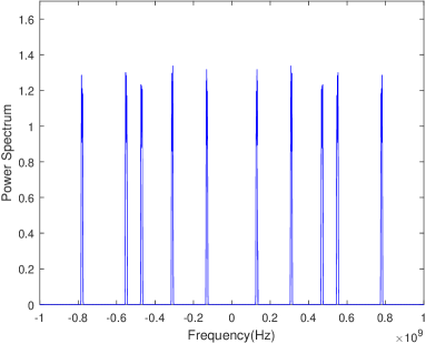
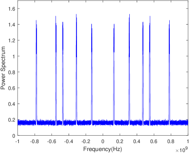
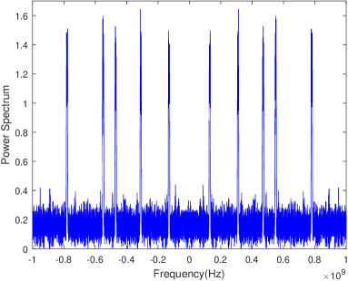
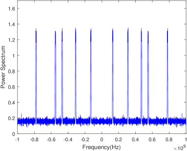
In our experiments, we generate $5$ wide-sense stationary signals within the frequency range $[0,1]$GHz by filtering the zero-mean unit-variance Gaussian white noise using band-pass FIR filters. Our objective is to identify the frequency locations of the signals that spread over the frequency band $[0,1]$GHz. Clearly, the Nyquist sampling rate is $2$GHz. The bandwidth of each signal component is set to $10$MHz and their carrier frequencies are set to $130$, $310$, $470$, $550$, and $780$MHz, respectively. For our proposed method, a multicoset sampling scheme is employed to collect sub-Nyquist data samples, in which the number of sampling channels is set to $M=8$, the sampling rate for each channel is set to $80$MHz and the time delays are set to $\{0,0.5,1,1.5,2,2.5,3,6.5\}$ nanoseconds (ns). The downsampling factor is equal to $N=f_{nyq}/(80\text{MHz})=25$. The spectrum resolution is set to $62.5$kHz, which corresponds to a power spectrum of length $32000$. Hence, we have $2NL\geq 32000$ and each sampling channel needs to collect $L\geq 32000/2N=640$ data samples. In our experiments, we collect data samples of $1$ms’ duration for each channel. We then calculate the autocorrelation sequence and truncate it to a vector of length $32000$. For our proposed method and the conventional time-domain algorithm [18], a hamming window is added to the estimated autocorrelation sequence to enhance the power spectrum estimation accuracy.

Fig. 5 plots the power spectrum reconstructed using noiseless Nyquist data samples collected within $1$ms, using noisy Nyquist data samples collected within $1$ms, the power spectrum reconstructed via our proposed method with noisy sub-Nyquist data samples collected within $1$ms, and noisy sub-Nyquist data samples collected within $10$ms, where the signal to noise ratio (SNR) is set to -5dB for the noisy scenario. The noisy signal is generated by corrupting the original signal $x(t)$ with zero mean Gaussian noise. The SNR is defined as

$$\text{SNR}=10\log_{10}\frac{\sum_{n=1}^{N_{t}}|x[n]|^{2}}{N_{t}\sigma^{2}},$$ (55)

where $\{x[n]\}$ denote the Nyquist samples of $x(t)$, $N_{t}$ is the number of the Nyquist samples, and $\sigma^{2}$ denotes the variance of the Gaussian noise. From Fig. 5, we see that our proposed method is able to accurately recover the true power spectrum. Specifically, the normalized mean square errors (NMSE), $E[\|\boldsymbol{s}-\boldsymbol{\hat{s}}\|_{2}^{2}/\|\boldsymbol{s}\|_{2}^{2}]$, for Fig. 5(b)–(d) are respectively given as $0.0057$, $0.0377$, and $0.0037$, where $\boldsymbol{s}$ and $\boldsymbol{\hat{s}}$ denotes the groundtruth and estimated power spectrum, respectively. Moreover, we observe that, with sub-Nyquist samples collected within $10$ms, our proposed method provides an accuracy slightly higher than that obtained using $1$ms Nyquist samples. This result implies that the performance loss caused by downsampling can be compensated by increasing the sampling time.

Figure 6: TPR vs. FPR for different SNRs.

Figure 7: TPR vs. FPR under different compression ratios.

Figure 8: The ROC of our proposed method and the frequency-domain method. The run times of our proposed method and the frequency-domain method are $0.17s$ and $0.35s$, respectively.

Figure 9: The ROC of our proposed method and the time-domain method. The run times of our proposed method and the time-domain method are $0.03s$ and $0.13s$, respectively.

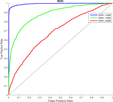
To more fully examine the performance, we plot the ROC curve for our proposed method under different SNRs in Fig. 6. The ROC curve is created by plotting the true positive rate (TPR) against the false positive rate (FPR) at various threshold settings. Specifically, given an estimated power spectrum, one can use a threshold to identify the frequency locations of the signals that spread over a wide frequency band, i.e. those grid points which have a higher energy level than the threshold are considered positive, otherwise it is considered that no signals reside on those grid points. The TPR and the FPR can be calculated by comparing the detection result and the groundtruth. The ROC curve can then be obtained by trying different thresholds. From Fig. 6, we see that our proposed method can achieve reliable detection even in the low SNR regime, say, $\text{SNR}=-10\text{dB}$. This result demonstrates the superiority of the use of statistical information for spectrum sensing. Such a merit is particularly useful for wideband spectrum sensing because, to obtain a practically meaningful receiver sensitivity (typical value for the receiver sensitivity is around $-70\sim-90$dBm), the receiver has to operate in a low SNR regime. To illustrate this, note that the receiver sensitivity can be calculated as

$$S=10\log(kT_{\text{syst}})+10\log(B)+NF_{RX}+\text{SNR},$$ (56)

where $10\log(kT_{\text{syst}})$ is equal to -174dBm/Hz for a system temperature of 17 degrees in Celsius, $B$ is the bandwidth of the signal in hertz, and $NF_{RX}$ is the noise figure of the receiver in decibels whose typical value is 6dB [32]. Thus the receiver sensitivity is given by $S=-174\text{dBm/Hz}+10\log(1\text{GHz})+6\text{dB}+\text{SNR}=-78\text{dBm}+\text{SNR}$. To achieve a receiver sensitivity of $-80$dBm, the SNR is equal to $-80-(-78)=-2\text{dB}$ for this typical scenario.

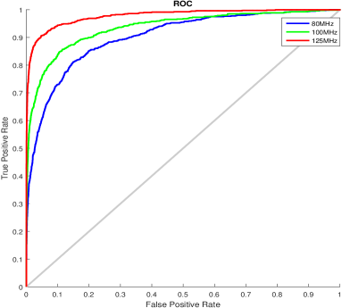
Next, we study the performance of our proposed method under different compression ratios. We consider cases where the sampling rate of the ADCs are set to 80MHz, 100MHz, and 125MHz, respectively. Accordingly, the downsampling factor $N$ is equal to $25$, $20$, and $16$, respectively, and the compression ratio equals 0.32, 0.4, and 0.5, respectively. We plot the ROC curve in Fig. 7, where the SNR is set to -20dB. From Fig. 7, we see that the performance can be considerably improved as the sampling rate increases.

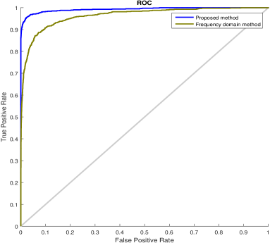
To show the computational efficiency, we report the average run times of the proposed method and the frequency-domain approach. For the frequency-domain approach, the MWC consists of 8 sampling channels. In each channel, the signal is first modulated by a periodic PN sequence with a period of $12.5$ns (i.e. $N=25$), then filtered using an ideal low-pass filter with a cutoff frequency of $40$MHz, and finally sampled by an ADC with a sampling rate of $80$MHz. We note that the MWC and the multicoset sampling scheme have the same number of channels as well as the same sampling rate per channel. Thus the comparison is fair. For both methods, we collect data samples within an interval of $1$ms. We consider two cases where the frequency resolution is set to $62.5$kHz and $125$kHz, respectively. The experiments are conducted using MATLAB R2015b under a laptop with 2.5GHz Intel i7 CPU and 16G RAM. We report the average run times as well as the ROC curve in Fig. 8. From Fig. 8, we see that our proposed method achieves better performance than the frequency-domain approach. Such a performance improvement is due to the fact that for our proposed method which explicitly estimates the autocorrelation of the original signal, a hamming window can be added to the estimated autocorrelation sequence to enhance the power spectrum estimation accuracy. Besides, from the reported run times, we see that the proposed method takes about half the time needed by the frequency-domain approach for power spectrum reconstruction. Such an advantage in terms of the computational complexity would be more significant for practical FPGA-based systems as our proposed method which involves FFT operations can be more efficiently implemented.

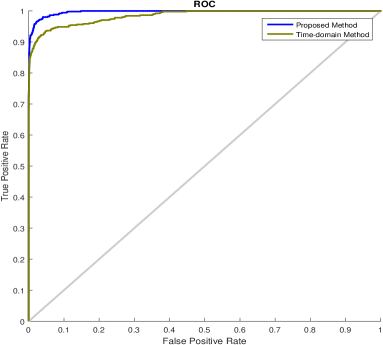
We also compare our proposed method with the conventional time-domain method [18]. For a fair comparison, we assume that the multicoset sampling scheme is used by the time-domain method to collect sub-Nyquist samples. The number of sampling channels and the time delay parameters are the same as described earlier. To relieve the large amount of memory required by the conventional time-domain method, the frequency resolution is set to 1MHz. The SNR is set to -12dB in our experiments. We collect data samples within 0.1ms. Average run times and ROC curves are reported in Fig. 9. From Fig. 9, we see that our proposed method runs faster than the conventional time-domain method. Besides, we observe that our proposed method slightly outperforms the time-domain method, which is possibly due to the fact that to calculate the correlation matrix, the conventional time-domain method needs to divide the collected data samples into a number of segments and neglects the correlation between different segments, while our proposed method deals with all the data samples in a batch and thus is able to obtain a better autocorrelation estimation.

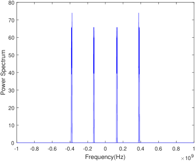
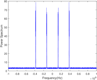
Note that our proposed method is able to reconstruct the power spectrum without placing any sparsity constraint on the spectrum under monitoring. To show this, we consider a multi-band signal which consists of 32 narrowband components within the frequency range $[0,1]$GHz. The narrowband components are generated by passing the white Gaussian noise through band-pass FIR filters. The bandwidth of each narrowband signal is set to 20MHz. The center frequencies of these narrowband signals are uniformly distributed so that no narrowband signals overlap each other. The spectral occupancy ratio can be easily calculated as $(32\times 20\text{MHz})/(1\text{GHz})=64\%$, which indicates that the power spectrum under monitoring is non-sparse. The sampling setup is the same as that used in our previous examples, in which we use $M=8$ branches and the sampling rate per channel is set to $80$MHz. Fig. 10 shows the estimated power spectrum using noiseless sub-Nyquist samples collected within 10ms. For a comparison, the power spectrum estimated using noiseless Nyquist samples collected within 1ms is also included. The NMSEs of the reconstructed power spectrum for Fig. 10(a)–(b) are respectively given as $0.0055$ and $0.0014$. From Fig. 10, we see that although the spectrum under monitoring is non-sparse, our proposed method still provides a reliable estimate of the original power spectrum.

Figure 10: From left to right: Power spectrum reconstructed using noiseless Nyquist samples collected within 1ms; Power spectrum reconstructed via our proposed method with 10ms noiseless sub-Nyquist samples.

IV-B Results on Cyclostationary Signals

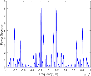
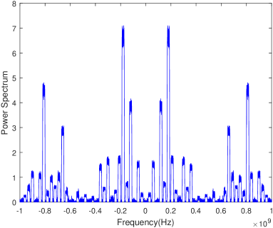
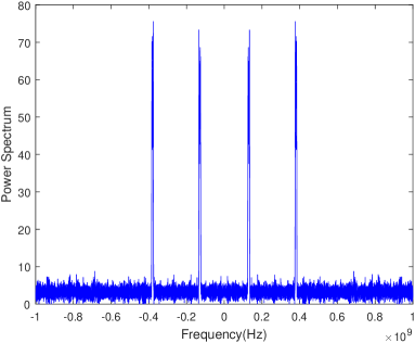
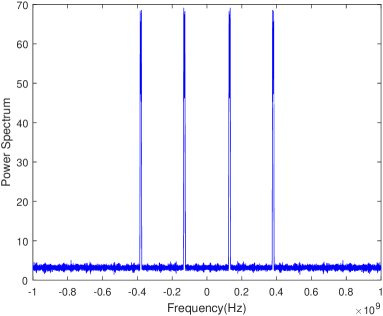
To show that the proposed method is applicable to cyclostationary signals, we generate two communication signals, namely, a BPSK signal and a QAM16 signal, which are known to be cyclostationary, within the frequency range $[0,1]$GHz. The carrier frequencies of these two signals are set to 130MHz and 380MHz, respectively, and their symbol rates are set to 10M symbols per second. The SNR is set to -5dB and the multicoset sampling architecture has the same setup as that mentioned earlier in this section. Fig. 11 shows the estimated power spectra using noisy data samples collected within 1ms and 10ms, from which we see that our proposed method can yield an accurate power spectrum estimate of cyclostationary signals.

(a)

(b)

(c)

(d)

Figure 11: (a) Power spectrum reconstructed using noiseless Nyquist samples collected within 1ms; (b) Power spectrum reconstructed using noisy Nyquist samples collected within 1ms; (c) Power spectrum reconstructed via our proposed method with 1ms noisy sub-Nyquist samples; (d) Power spectrum reconstructed via our proposed method with 10ms noisy sub-Nyquist samples.

V Conclusions

In this paper, we studied the problem of compressed power spectrum estimation which aims to reconstruct the power spectrum of a wide-sense stationary multi-band signal based on sub-Nyquist samples. By exploiting the sampling structure of the multicoset sampling scheme, we developed a fast compressed power spectrum estimation method. The proposed method has a lower computational complexity than existing methods, and can be efficiently implemented in practical systems as its primary computational task consists of FFT operations. Simulation results were provided to illustrate the computational efficiency and effectiveness of our proposed method.

Appendix A Proof of Lemma 1

We only need to show that for any $k\in[-LN+1,LN-1]$, there exists at least one $n\in[0,LN-1]$ such that $I[n]I[n-k]=1$. Note that $\{I[n]\}$ is a periodic sequence with period $N$. Hence if $I[n]I[n-k]=1$, then for any integer $a$ such that $n-k+aN\in[0,LN-1]$, we also have $I[n]I[n-k+aN]=1$. In other words, if $Q_{k}>0$, then $Q_{k+aN}>0$. Therefore we only need to examine $k$ in the range of $|k|\leq\lfloor N/2\rfloor$. Recall that for any $|k|\leq\lfloor N/2\rfloor$, there exists $m_{1},m_{2}$ and $c\in\{-1,0,1\}$ such that

$$k=\Delta_{m_{1}}-\Delta_{m_{2}}+cN.$$ (57)

Set $n=\Delta_{m_{1}}+c^{\prime}N$ and $n-k=\Delta_{m_{2}}+(c+c^{\prime})N$, where $c^{\prime}$ is an integer such that $n\in[0,LN-1]$ and $n-k\in[0,LN-1]$. According to the definition of $I[n]$, it is easy to know that $I[\Delta_{m_{1}}+c^{\prime}N]=I[\Delta_{m_{2}}+(c+c^{\prime})N]=1$. Consequently, we have $I[n]I[n-k]=1$ and thus $Q_{k}>0$.

References

- [1] M. R. Palattella, M. Dohler, A. Grieco, G. Rizzo, J. Torsner, T. Engel, and L. Ladid, “Internet of things in the 5G era: Enablers, architecture, and business models,” IEEE Journal on Selected Areas in Communications, vol. 34, no. 3, pp. 510–527, 2016.
- [2] M. Song, C. Xin, Y. Zhao, and X. Cheng, “Dynamic spectrum access: from cognitive radio to network radio,” IEEE Wireless Communications, vol. 19, no. 1, pp. 23–29, 2012.
- [3] T. Yucek and H. Arslan, “A survey of spectrum sensing algorithms for cognitive radio applications,” IEEE communications surveys & tutorials, vol. 11, no. 1, pp. 116–130, 2009.
- [4] E. Axell, G. Leus, E. G. Larsson, and H. V. Poor, “Spectrum sensing for cognitive radio: State-of-the-art and recent advances,” IEEE Signal Processing Magazine, vol. 29, no. 3, pp. 101–116, May 2012.
- [5] P. Wang, J. Fang, N. Han, and H. Li, “Multiantenna-assisted spectrum sensing for cognitive radio,” IEEE Transactions on Vehicular Technology, vol. 59, no. 4, pp. 1791–1800, May 2010.
- [6] H. Sun, A. Nallanathan, C.-X. Wang, and Y. Chen, “Wideband spectrum sensing for cognitive radio networks: a survey,” IEEE Wireless Communications, vol. 20, no. 2, pp. 74–81, Apr. 2013.
- [7] F. Wang, J. Fang, H. Duan, and H. Li, “Phased-array-based sub-nyquist sampling for joint wideband spectrum sensing and direction-of-arrival estimation,” IEEE Trans. Signal Processing, vol. 66, no. 23, pp. 6110–6123, Dec. 2018.
- [8] D. L. Donoho, “Compressive sensing,” IEEE Transactions on Information Theory, vol. 52, pp. 1289–1306, 2006.
- [9] E. Candés, J. Romberg, and T. Tao, “Robust uncertainty principles: exact signal reconstruction from highly incomplete frequency information,” IEEE Trans. Inform. Theory, vol. 52, no. 2, pp. 489–509, Feb. 2006.
- [10] M. Mishali and Y. C. Eldar, “From theory to practice: Sub-Nyquist sampling of sparse wideband analog signals,” IEEE Journal of Selected Topics in Signal Processing, vol. 4, no. 2, pp. 375–391, Apr. 2010.
- [11] Z. Zhang, Z. Han, H. Li, D. Yang, and C. Pei, “Belief propagation based cooperative compressed spectrum sensing in wideband cognitive radio networks,” IEEE Transactions on Wireless communications, vol. 10, no. 9, pp. 3020–3031, Sept. 2011.
- [12] M. Wakin, S. Becker, E. Nakamura, M. Grant, E. Sovero, D. Ching, J. Yoo, J. Romberg, A. Emami-Neyestanak, and E. Candès, “A nonuniform sampler for wideband spectrally-sparse environments,” IEEE Journal on Emerging and Selected Topics in Circuits and Systems, vol. 2, no. 3, pp. 516–529, Sept. 2012.
- [13] M. Mishali, Y. C. Eldar, and A. J. Elron, “Xampling: Signal acquisition and processing in union of subspaces,” IEEE Transactions on Signal Processing, vol. 59, no. 10, pp. 4719–4734, 2011.
- [14] H. Sun, W.-Y. Chiu, J. Jiang, A. Nallanathan, and H. V. Poor, “Wideband spectrum sensing with sub-Nyquist sampling in cognitive radios,” IEEE Trans. Signal Processing, vol. 60, no. 11, pp. 6068–6073, Nov. 2012.
- [15] Z. Qin, Y. Gao, M. D. Plumbley, and C. G. Parini, “Wideband spectrum sensing on real-time signals at sub-Nyquist sampling rates in single and cooperative multiple nodes,” IEEE Trans. Signal Processing, vol. 64, no. 12, pp. 3106–3117, June 2016.
- [16] B. Khalfi, B. Hamdaoui, M. Guizani, and N. Zorba, “Efficient spectrum availability information recovery for wideband dsa networks: A weighted compressive sampling approach,” IEEE Transactions on Wireless Communications, vol. 17, no. 4, pp. 2162–2172, Apr. 2018.
- [17] Z. Tian, Y. Tafesse, and B. M. Sadler, “Cyclic feature detection with sub-nyquist sampling for wideband spectrum sensing,” IEEE Journal of Selected Topics in Signal Processing, vol. 6, no. 1, pp. 58–69, Feb. 2012.
- [18] D. D. Ariananda and G. Leus, “Compressive wideband power spectrum estimation,” IEEE Trans. Signal Processing, vol. 60, no. 9, pp. 4775–4789, Sept. 2012.
- [19] C.-P. Yen, Y. Tsai, and X. Wang, “Wideband spectrum sensing based on sub-nyquist sampling,” IEEE Transactions on Signal Processing, vol. 61, no. 12, pp. 3028–3040, June 2013.
- [20] D. Cohen and Y. C. Eldar, “Sub-Nyquist sampling for power spectrum sensing in cognitive radios: A unified approach,” IEEE Trans. Signal Processing, vol. 62, no. 15, pp. 3897–3910, Aug. 2014.
- [21] E. Lagunas and M. Nájar, “Spectral feature detection with sub-nyquist sampling for wideband spectrum sensing,” IEEE Transactions on Wireless Communications, vol. 14, no. 7, pp. 3978–3990, July 2015.
- [22] D. Romero, D. D. Ariananda, Z. Tian, and G. Leus, “Compressive covariance sensing: Structure-based compressive sensing beyond sparsity,” IEEE Signal Processing Magazine, vol. 33, no. 1, pp. 78–93, Jan. 2016.
- [23] J. N. Laska, S. Kirolos, M. F. Duarte, T. S. Ragheb, R. G. Baraniuk, and Y. Massoud, “Theory and implementation of an analog-to-information converter using random demodulation,” in 2007 IEEE International Symposium on Circuits and Systems. IEEE, 2007, pp. 1959–1962.
- [24] R. Venkataramani and Y. Bresler, “Optimal sub-Nyquist nonuniform sampling and reconstruction for multiband signals,” IEEE Transactions on Signal Processing, vol. 49, no. 10, pp. 2301–2313, 2001.
- [25] M. Mishali and Y. C. Eldar, “Blind multi-band signal reconstruction: compressed sensing for analog signals,” IEEE Trans. Signal Processing, vol. 57, no. 3, pp. 993–1009, Mar. 2009.
- [26] D. Romero and G. Leus, “Compressive covariance sampling,” in Information Theory and Applications Workshop (ITA), San Diego, CA, USA, February 10-15 2013.
- [27] N. González-Prelcic and M. E. Domínguez-Jiménez, “Circular sparse rulers based on co-prime sampling for compressive power spectrum estimation,” in 2014 IEEE Global Communications Conference, Austin, United of States, Dec. 2014, pp. 3044–3050.
- [28] M. Domínguez-Jiménez and N. González-Prelcic, “A class of circular sparse rulers for compressive power spectrum estimation,” in 21st European Signal Processing Conference (EUSIPCO 2013), Palais des Congrés, Marrakech, Sept. 2013, pp. 1–5.
- [29] P. Feng and Y. Bresler, “Spectrum-blind minimum-rate sampling and reconstruction of multiband signals,” in IEEE International Conference on Acoustics, Speech, and Signal Processing Conference Proceedings, Atlanta, GA, USA, May 9 1996.
- [30] J. G. Proakis, Digital signal processing: principles algorithms and applications. Pearson Education India, 2001.
- [31] Xilinx, “Logicore ip fast fourier transform v8.0.” [Online]. Available: https://www.xilinx.com/support/documentation/ip˙documentation/ds808˙xfft.pdf
- [32] M. Integrated, “System noise-figure analysis for modern radio receivers.” [Online]. Available: https://pdfserv.maximintegrated.com/en/an/TUT5594.pdf