Comparison of numerical methods for the nonlinear Klein-Gordon equation in the nonrelativistic limit regime

Abstract

Different efficient and accurate numerical methods have recently been proposed and analyzed for the nonlinear Klein-Gordon equation (NKGE) with a dimensionless parameter $\varepsilon\in(0,1]$, which is inversely proportional to the speed of light. In the nonrelativestic limit regime, i.e. $0<\varepsilon\ll 1$, the solution of the NKGE propagates waves with wavelength at $O(1)$ and $O(\varepsilon^{2})$ in space and time, respectively, which brings significantly numerical burdens in designing numerical methods. We compare systematically spatial/temporal efficiency and accuracy as well as $\varepsilon$-resolution (or $\varepsilon$-scalability) of different numerical methods including finite difference time domain methods, time-splitting method, exponential wave integrator, limit integrator, multiscale time integrator, two-scale formulation method and iterative exponential integrator. Finally, we adopt the multiscale time integrator to study the convergence rates from the NKGE to its limiting models when $\varepsilon\to 0^{+}$.

1 Introduction

Consider the dimensionless nonlinear Klein-Gordon equation (NKGE) in $d$-dimensions ($d=1,2,3$) with cubic nonlinearity [10, 11, 30, 35, 49]:

$$\left\{\begin{split}&\varepsilon^{2}\partial_{tt}u(\mathbf{x},t)-\Delta u(\mathbf{x},t)+\frac{1}{\varepsilon^{2}}u(\mathbf{x},t)+\lambda\,|u(\mathbf{x},t)|^{2}u(\mathbf{x},t)=0,\quad\mathbf{x}\in\mathbb{R}^{d},\quad t>0,\\ &u(\mathbf{x},0)=\phi_{1}(\mathbf{x}),\quad\partial_{t}u(\mathbf{x},0)=\frac{1}{\varepsilon^{2}}\phi_{2}(\mathbf{x}),\quad\mathbf{x}\in\mathbb{R}^{d},\end{split}\right.$$ (1.1)

where $t$ is time, $\mathbf{x}\in\mathbb{R}^{d}$ is the spatial coordinate, $u:=u(\mathbf{x},t)$ is a complex-valued scalar field, $0<\varepsilon\leq 1$ is a dimensionless parameter inversely proportional to the speed of light, $\lambda\in\mathbb{R}$ is a given dimensionless parameter (positive and negative for defocusing and focusing self-interaction, respectively), and $\phi_{1}$ and $\phi_{2}$ are given complex-valued $\varepsilon$-independent initial data.

When $\lambda=0$, the above Klein-Gordon equation is known as the relativistic version of the Schrödinger equation for correctly describing the spinless relativistic composite particles, like the pion and the Higgs boson [35]. When $\lambda\neq 0$, the NKGE was widely adapted in plasma physics for modeling interaction between Langmuir and ion sound waves [21, 38] and in cosmology as a phonological model for dark-matter and/or black-hole evaporation [53, 75]. The NKGE (1.1) is time symmetric and conserves the energy

$$E(t) :=\int_{\mathbb{R}^{d}}\left[\varepsilon^{2}|\partial_{t}u(\mathbf{x},t)|^{2}+|\nabla u(\mathbf{x},t)|^{2}+\frac{1}{\varepsilon^{2}}|u(\mathbf{x},t)|^{2}+\frac{\lambda}{2}|u(\mathbf{x},t)|^{4}\right]d\mathbf{x}$$

$$\equiv\int_{\mathbb{R}^{d}}\left[\frac{1}{\varepsilon^{2}}|\phi_{2}(\mathbf{x})|^{2}+|\nabla\phi_{1}(\mathbf{x})|^{2}+\frac{1}{\varepsilon^{2}}|\phi_{1}(\mathbf{x})|^{2}+\frac{\lambda}{2}|\phi_{1}(\mathbf{x})|^{4}\right]d\mathbf{x}=E(0),\qquad t\geq 0.$$ (1.2)

For the derivation and nondimensionlization of (1.1), we refer to [11, 35, 61, 62] and references therein. For the well-posedness of the Cauchy problem (1.1) with a fixed $\varepsilon\in(0,1]$, e.g. $\varepsilon=1$, we refer to [35, 61, 62] and references therein. We remark here that when the initial data $\phi_{1}$ and $\phi_{2}$ are real-valued, then the solution $u$ of (1.1) is also real-valued; and this case has been widely studied analytically and numerically in the literature [1, 3, 22, 30, 36, 37, 41, 45, 46, 49, 54, 55, 56, 58, 59, 73, 72]. For simplicity of notations and without loss of generality, from now on, we assume that $\phi_{1}$ and $\phi_{2}$ are real-valued, and thus the solution $u$ of (1.1) is real-valued too. Our methods and results can be straightforwardly extended to the case when $\phi_{1}$ and $\phi_{2}$ are complex-valued and/or general nonlinearity in (1.1) [10, 11], and the conclusion will be remained the same.

When $\varepsilon\to 0^{+}$ in (1.1), due to that the energy $E(t)=O(\varepsilon^{-2})$ in (1) becomes unbounded, the analysis of the nonrelativistic limit of the solution $u$ becomes challenging and quite complicated. Fortunately, convergence from the NKGE (1.1) to a nonlinear Schrödinger equation has been extensively studied in the mathematics literature [10, 61, 62, 65]. Based on their results, the solution $u$ of the NKGE (1.1) propagates waves with wavelength at $O(\varepsilon^{2})$ and $O(1)$ in time and space, respectively, in the nonrelativistic limit regime, i.e. $0<\varepsilon\ll 1$. To illustrate this, Figure 1 shows the solution of (1.1) with $d=1$ and $\lambda=1$ and the initial data

$$\phi_{1}(x)=\frac{3\sin(x)}{e^{x^{2}/2}+e^{-x^{2}/2}},\qquad\phi_{2}(x)=\frac{2e^{-x^{2}}}{\sqrt{\pi}},\qquad x\in{\mathbb{R}}.$$ (1.3)

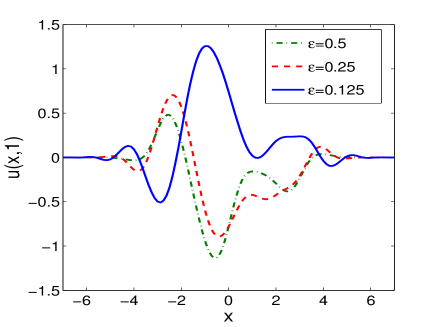
Figure 1: Solution of the NKGE (1.1) with $d=1$, $\lambda=1$ and the initial data taken as (1.3) for different $\varepsilon$.

In fact, when $0<\varepsilon\ll 1$, formally by taking the ansatz [61, 62]

$$u(\mathbf{x},t)=e^{it/\varepsilon^{2}}z(\mathbf{x},t)+e^{-it/\varepsilon^{2}}\overline{z}(\mathbf{x},t)+O(\varepsilon^{2}),\qquad\mathbf{x}\in\mathbb{R}^{d},\quad t\geq 0,$$ (1.4)

where $z:=z(\mathbf{x},t)$ is a complex-valued function and $\overline{z}$ denotes the complex conjugate of $z$, the NKGE (1.1) can be formally reduced to – semi-limiting model – the nonlinear Schrödinger equation with wave operator (NLSW) under well-prepared initial data [4, 6]

$$\left\{\begin{split}&2i\partial_{t}z(\mathbf{x},t)+\varepsilon^{2}\partial_{tt}z(\mathbf{x},t)-\Delta z(\mathbf{x},t)+3\lambda|z(\mathbf{x},t)|^{2}z(\mathbf{x},t)=0,\qquad\mathbf{x}\in\mathbb{R}^{d},\quad t>0,\\ &z(\mathbf{x},0)=\frac{1}{2}\left[\phi_{1}(\mathbf{x})-i\phi_{2}(\mathbf{x})\right]=:z_{0}(\mathbf{x}),\qquad\mathbf{x}\in\mathbb{R}^{d},\\ &\partial_{t}z(\mathbf{x},0)=\frac{i}{2}\left[-\Delta z_{0}(\mathbf{x})+3\lambda|z_{0}(\mathbf{x})|^{2}z_{0}(\mathbf{x})\right].\end{split}\right.$$ (1.5)

In addition, by dropping the small term $\varepsilon^{2}\partial_{tt}z$ in (1.5), one gets – limiting model – the nonlinear Schrödinger equation (NLSE) [4, 6, 61, 62]

$$\left\{\begin{split}&2i\partial_{t}z(\mathbf{x},t)-\Delta z(\mathbf{x},t)+3\lambda|z(\mathbf{x},t)|^{2}z(\mathbf{x},t)=0,\qquad\mathbf{x}\in\mathbb{R}^{d},\quad t>0,\\ &z(\mathbf{x},0)=\frac{1}{2}\left[\phi_{1}(\mathbf{x})-i\phi_{2}(\mathbf{x})\right]:=z_{0}(\mathbf{x}),\qquad\mathbf{x}\in\mathbb{R}^{d}.\end{split}\right.$$ (1.6)

When $\varepsilon=1$ in (1.1), i.e. $O(1)$-wave speed regime, several numerical methods have been proposed and analyzed for the Cauchy problem (1.1) in the literature, see [22, 41, 60, 55, 59, 73] and references therein. Specifically, the finite difference time domain (FDTD) methods [41, 55, 72] have been demonstrated excellent performance in terms of efficiency and accuracy for (1.1) when $\varepsilon=1$. However, when $0<\varepsilon\ll 1$, i.e. in the nonrelativistic limit regime, it becomes much more challenging in designing and analyzing efficient and accurate numerical methods for (1.1) due to the highly oscillatory nature of the solution in time (cf. Fig. 1). To address this issue, Bao and Dong [11] established rigorous error bounds of the FDTD methods for (1.1), which depends explicitly on the mesh size $h$ and time step $\tau$ as well as the small parameter $\varepsilon\in(0,1]$. Based on their results [11], in order to obtain the ‘correct’ numerical solution of (1.1), the $\varepsilon$-resolution (or $\varepsilon$-scalability or meshing strategy) of the FDTD methods is $\tau=O(\varepsilon^{3})$ and $h=O(1)$, which is under-resolution in time with respect to $\varepsilon\in(0,1]$ regarding to the Shannon’s information theory [57, 68, 69] – to resolve a wave one needs a few points per wavelength – since the wavelength in time is at $O(\varepsilon^{2})$. To overcome the temporal under-resolution of the FDTD methods, they [11] proposed to adapt the exponential wave integrator (EWI) [52] for discretizing temporal derivatives in (1.1) and showed rigorously the $\varepsilon$-resolution of EWI is $\tau=O(\varepsilon^{2})$ and $h=O(1)$, which is optimal-resolution in time with respect to $\varepsilon\in(0,1]$. Later, the time-splitting (TS) method [63] was also applied to discretize the NKGE (1.1), and the method was shown as equivalent to one type EWI and thus it retains the same $\varepsilon$-resolution as that of the EWI but with an improved error bound regarding to the small parameter $\varepsilon\in(0,1]$ [40]. In fact, FDTD, EWI and TS methods perform very well when $\tau\to 0$ under $\varepsilon=\varepsilon_{0}$ fixed and they lose accuracy when $\varepsilon\to 0$ under $\tau=\tau_{0}$ fixed. At the meantime, Faou and Schratz [42] presented a class of limit integrators (LI) for (1.1) via solving numerically the limiting model NLSE (1.6) and obtained their error bounds. On the contrary, the LI methods perform very well when $\varepsilon\to 0$ under $\tau=\tau_{0}$ fixed and they lose accuracy when $\tau\to 0$ under $\varepsilon=\varepsilon_{0}$ fixed.

It is a natural question to ask on whether one can design a numerical method for the NKGE (1.1) such that it is uniformly accurate for $\varepsilon\in(0,1]$, i.e. super-resolution in time, especially in the nonrelativistic limit regime, since we have the solution structure (1.4) of the NKGE (1.1) via the limiting model NLSW (1.5) or NLSE (1.6). Recently, different uniformly accurate (UA) numerical methods have been designed and analyzed for the NKGE (1.1) including a multiscale time integrator (MTI) via a multiscale decomposition of the solution [10] and a two-scale formulation (TSF) method [26] as well as two uniformly and optimally accurate (UOA) methods [19, 20]. The main aim of this paper is to carry out a systematical comparison of different numerical methods which have been proposed for the NKGE (1.1) in terms of temporal/spatial accuracy and efficiency as well as $\varepsilon$-resolution for $\varepsilon\in(0,1]$, especially in the nonrelativistic limit regime.

The rest of the paper is organized as follows. The FDTD, EWI and TS methods as well as the LI schemes for the NKGE (1.1) are briefly reviewed in Section 2; the uniformly accurate methods are briefly reviewed in Section 3; and the uniformly and optimally accurate methods are briefly reviewed in Section 4. In Section 5, we present detailed comparison of different numerical methods; and in Section 6, we report convergence rates of the NKGE (1.1) to its limiting models NLSW (1.5) and NLSE (1.6) and show wave interactions of NKGE in two dimensions (2D). Finally, some conclusions are drawn in Section 7. Throughout this paper, we adopt the notation $A\lesssim B$ to represent that there exists a generic constant $C>0$, which is independent of $\tau$ (or $n$), $h$ and $\varepsilon$, such that $|A|\leq CB$.

2 Non-uniformly accurate numerical methods

In this section, we briefly review the FDTD, EWI and TS methods [11] as well as the LI methods [42] which have been proposed in the literature for discretizing the NKGE (2.1) (or (1.1)).

For simplicity of notation and without loss of generality, we only present the numerical methods in one dimension (1D). Generalization to high dimensions is straightforward by tensor product. As adapted in the literature [10, 20, 26], the NKGE (1.1) with $d=1$ is usually truncated onto a bounded interval $\Omega=(a,b)$ ($|a|$ and $b$ are usually taken large enough such that the truncation error is negligible) with periodic boundary condition

$$\left\{\begin{split}&\varepsilon^{2}\partial_{tt}u(x,t)-\partial_{xx}u(x,t)+\frac{1}{\varepsilon^{2}}u(x,t)+\lambda(u(x,t))^{3}=0,\qquad x\in\Omega,\quad t>0,\\ &u(x,0)=\phi_{1}(x),\qquad\partial_{t}u(x,0)=\frac{1}{\varepsilon^{2}}\phi_{2}(x),\qquad x\in\overline{\Omega},\\ &u(a,t)=u(b,t),\qquad\partial_{x}u(a,t)=\partial_{x}u(b,t).\end{split}\right.$$ (2.1)

Choose $\tau>0$ be the time step and $h=(b-a)/N$ be the mesh size with $N$ an even positive integer, denote the grid points as $x_{j}=a+jh$ for $j=0,1,\ldots,N$ and time steps as $t_{n}=n\tau$ for $n\geq 0$. Let $u_{j}^{n}$ be the numerical approximation of $u(x_{j},t_{n})$ for $0\leq j\leq N$ and $n\geq 0$ and $u^{n}=(u_{0}^{n},u_{1}^{n},\ldots,u_{N}^{n})^{T}$ be the solution vector at $t=t_{n}$, and define

$$\|u^{n}\|_{l^{2}}^{2}=h\sum_{j=0}^{N-1}|u_{j}^{n}|^{2},\qquad n\geq 0.$$ (2.2)

2.1 Finite difference time domain (FDTD) methods

Introduce the finite difference operators as

$$\delta_{t}^{2}u_{j}^{n}=\frac{u_{j}^{n+1}-2u_{j}^{n}+u_{j}^{n-1}}{\tau^{2}},\quad\delta_{x}^{+}u_{j}^{n}=\frac{u_{j+1}^{n}-u_{j}^{n}}{h},\quad\delta_{x}^{2}u_{j}^{n}=\frac{u_{j+1}^{n}-2u_{j}^{n}+u_{j-1}^{n}}{h^{2}}.$$

As used in [11], the Crank-Nicolson finite difference (CNFD) method for discretizing (2.1) reads

$$\varepsilon^{2}\delta_{t}^{2}u_{j}^{n}+\left[-\frac{1}{2}\delta_{x}^{2}+\frac{1}{2\varepsilon^{2}}+\frac{\lambda}{4}[(u_{j}^{n+1})^{2}+(u_{j}^{n-1})^{2}]\right](u_{j}^{n+1}+u_{j}^{n-1})=0,\quad 0\leq j\leq N-1,\quad n\geq 0.$$ (2.3)

Similarly, the semi-implicit finite difference (SIFD) method is [11]

$$\varepsilon^{2}\delta_{t}^{2}u_{j}^{n}-\frac{1}{2}\delta_{x}^{2}(u_{j}^{n+1}+u_{j}^{n-1})+\frac{1}{2\varepsilon^{2}}(u_{j}^{n+1}+u_{j}^{n-1})+\lambda(u_{j}^{n})^{3}=0,\quad 0\leq j\leq N-1,\quad n\geq 0;$$ (2.4)

and the leap-frog finite difference (LFFD) method is [11]

$$\varepsilon^{2}\delta_{t}^{2}u_{j}^{n}-\delta_{x}^{2}u_{j}^{n}+\frac{1}{\varepsilon^{2}}u_{j}^{n}+\lambda(u_{j}^{n})^{3}=0,\quad 0\leq j\leq N-1,\quad n\geq 0.$$ (2.5)

The initial and boundary conditions in (2.1) are discretized as [11, 13]

$$\begin{split}&u_{0}^{n}=u_{N}^{n},\quad u_{-1}^{n}=u_{N-1}^{n},\quad n\geq 0;\qquad u_{j}^{0}=\phi_{1}(x_{j}),\quad j=0,\ldots,N,\\ &u_{j}^{1}=\phi_{1}(x_{j})+\sin\left(\frac{\tau}{\varepsilon^{2}}\right)\phi_{2}(x_{j})+\frac{\tau}{2}\sin\left(\frac{\tau}{\varepsilon^{2}}\right)\left[\delta_{x}^{2}\phi_{1}(x_{j})-\frac{1}{\tau}\sin\left(\frac{\tau}{\varepsilon^{2}}\right)\phi_{1}(x_{j})-\lambda(\phi_{1}(x_{j}))^{3}\right].\end{split}$$ (2.6)

We remark here that we adapt (2.6) to compute the approximation at $t=t_{1}$ instead of the classical method

$$u_{j}^{1}=\phi_{1}(x_{j})+\frac{\tau}{\varepsilon^{2}}\phi_{2}(x_{j})+\frac{\tau^{2}}{2\varepsilon^{2}}\left[\delta_{x}^{2}\phi_{1}(x_{j})-\frac{1}{\varepsilon^{2}}\phi_{1}(x_{j})-\lambda(\phi_{1}(x_{j}))^{3}\right],\qquad j=1,2,\ldots,N-1,$$ (2.7)

i.e. replacing $\tau/\varepsilon^{2}$ by $\sin(\tau/\varepsilon^{2})$, such that the numerical solution $u^{1}$ is uniformly bounded for $\varepsilon\in(0,1]$.

As observed and stated in [11], the above CNFD, SIFD and LFFD methods are time symmetric and their memory cost is $O(N)$. The LFFD method is explicit and its computational cost per step is $O(N)$. It is conditionally stable and there is a severe stability condition which depends on both $h$ and $\varepsilon$, especially when $0<\varepsilon\ll 1$ [11]. In fact, it is the most efficient and accurate method among all FDTD methods for the NKGE when $\varepsilon=1$. The SIFD method is implicit, but it can be solved efficiently via the fast Fourier transform (FFT) and thus its computational cost per step is $O(N\,\ln N)$. It is conditionally stable and the stability condition depends on $\varepsilon$ and is independent of $h$ [11]. The CNFD method is implicit and at every time step a fully nonlinear coupled system needs to be solved. One main advantage is that it conserves the energy (1) in the discrete level as [11]

$$E^{n} :=\varepsilon^{2}\|\delta_{t}^{+}u^{n}\|_{l^{2}}^{2}+\frac{1}{2}\left(\|\delta_{x}^{+}u^{n}\|_{l^{2}}^{2}+\|\delta_{x}^{+}u^{n+1}\|_{l^{2}}^{2}\right)+\frac{1}{2\varepsilon^{2}}\left(\|u^{n}\|_{l^{2}}^{2}+\|u^{n+1}\|_{l^{2}}^{2}\right)+\frac{h\lambda}{4}\sum_{j=0}^{N-1}\left[(u_{j}^{n})^{4}+(u_{j}^{n+1})^{4}\right]$$

$$\equiv E^{0},\qquad n\geq 0,$$ (2.8)

which immediately implies that it is unconditionally stable when $\lambda\geq 0$. In addition, under proper regularity of the solution $u$ of the NKGE (2.1) and stability conditions for the SIFD and LFFD methods, the following rigorous error bound was established for the three FDTD methods [11]

$$\|e^{n}\|_{l^{2}}+\|\delta_{x}^{+}e^{n}\|_{l^{2}}\lesssim h^{2}+\frac{\tau^{2}}{\varepsilon^{6}},\qquad 0\leq n\leq\frac{T}{\tau},$$ (2.9)

where $T>0$ is a fixed time and the error function $e^{n}$ is defined as $e_{j}^{n}=u(x_{j},t_{n})-u_{j}^{n}$ for $0\leq j\leq N$ and $n\geq 0$. This error bound suggests that the FDTD methods are second order in both space and time discretization for any fixed $\varepsilon=\varepsilon_{0}$ and the $\varepsilon$-resolution of the FDTD methods is $h=O(1)$ and $\tau=O(\varepsilon^{3})$ in the nonrelativistic limit regime, i.e. $0<\varepsilon\ll 1$, which immediately show that the temporal resolution with respect to $\varepsilon\in(0,1]$ of the FDTD methods is under-resolution in time since the wavelength in time is at $O(\varepsilon^{2})$.

2.2 Exponential wave integrator (EWI)

As it has been proposed in [11], the NKGE (2.1) is discretized in space by the Fourier (pseudo)spectral method and followed by adapting an exponential wave integrator (EWI) in time which has been widely used for discretizing second order oscillatory differential equations in the literature [31, 39, 44, 47, 48, 50, 51, 52].

Let $u_{j}^{n}$ and $\dot{u}_{j}^{n}$ be the approximations of $u(x_{j},t_{n})$ and $\partial_{t}u(x_{j},t_{n})$, respectively, for $0\leq j\leq N$ and $n\geq 0$ and take $u_{j}^{0}=\phi_{1}(x_{j}),\dot{u}_{j}^{0}=\phi_{2}(x_{j})/\varepsilon^{2}$ for $j=0,1,\ldots,N$. When the EWI is taken as the Gautschi’s quadrature [11, 44, 47, 48, 51], a Gautschi-type exponential wave integrator Fourier pseudospectral (EWI-FP) method [11] reads as:

$$u_{j}^{n+1}=\sum_{l=-N/2}^{N/2-1}\widetilde{(u^{n+1})}_{l}\;e^{i\mu_{l}(x_{j}-a)}=\sum_{l=-N/2}^{N/2-1}\widetilde{(u^{n+1})}_{l}\;e^{2ijl\pi/N},\qquad j=0,1,\ldots,N,\quad n\geq 0,$$ (2.10)

where

$$\widetilde{(u^{n+1})}_{l}=\left\{\begin{array}[]{ll}\left[\cos(\omega_{l}^{0}\tau)+\displaystyle\frac{\alpha^{0}\left(1-\cos(\omega_{l}^{0}\tau)\right)}{(\varepsilon\omega_{l}^{0})^{2}}\right]\widetilde{(u^{0})}_{l}+\displaystyle\frac{\sin(\omega_{l}^{0}\tau)}{\omega_{l}^{0}}\widetilde{(\dot{u}^{0})}_{l}+\displaystyle\frac{\cos(\omega_{l}^{0}\tau)-1}{(\varepsilon\omega_{l}^{0})^{2}}\widetilde{(f^{0})}_{l},&n=0,\\ \\ -\widetilde{(u^{n-1})}_{l}+2\left[\cos(\omega_{l}^{n}\tau)+\displaystyle\frac{\alpha^{n}\left(1-\cos(\omega_{l}^{n}\tau)\right)}{(\varepsilon\omega_{l}^{n})^{2}}\right]\widetilde{(u^{n})}_{l}+\displaystyle\frac{2\left(\cos(\omega_{l}^{n}\tau)-1\right)}{(\varepsilon\omega_{l}^{n})^{2}}\widetilde{(f^{n})}_{l},&n\geq 1,\\ \end{array}\right.$$

with $f(u)=\lambda u^{3}$, $f^{n}:=f(u^{n})=(f(u_{0}^{n}),f(u_{1}^{n}),\ldots,f(u_{N}^{n}))^{T}$, $\mu_{l}=2l\pi/(b-a)$, $\omega_{l}^{n}=\frac{1}{\varepsilon^{2}}\sqrt{1+\varepsilon^{2}(\mu_{l}^{2}+\alpha^{n})}$ ($l=-N/2,\ldots,N/2-1$) with $\alpha^{n}=\max\left\{\alpha^{n-1},\;\max_{0\leq j\leq N}\{\lambda(u_{j}^{n})^{2}\}\right\}$ for $n\geq 0$ and $\alpha^{-1}=0$ being the stabilization constants, and $\widetilde{v}_{l}$ ($-N/2\leq l\leq N/2-1$) being the discrete Fourier transform coefficients of the vector $v=(v_{0},v_{1},\ldots,v_{N})^{T}$ with $v_{0}=v_{N}$ defined as

$$\widetilde{v}_{l}=\frac{1}{N}\sum_{j=0}^{N-1}v_{j}\;e^{-i\mu_{l}(x_{j}-a)}=\frac{1}{N}\sum_{j=0}^{N-1}v_{j}\;e^{-2ijl\pi/N},\qquad l=-\frac{N}{2},-\frac{N}{2}+1,\ldots,\frac{N}{2}-1.$$ (2.11)

Of course, in practice if the approximation of the first order derivative in time is needed, then they can be obtained as [11]

$$\dot{u}_{j}^{n+1}=\sum_{l=-N/2}^{N/2-1}\widetilde{(\dot{u}^{n+1})}_{l}\ e^{i\mu_{l}(x_{j}-a)}=\sum_{l=-N/2}^{N/2-1}\widetilde{(\dot{u}^{n+1})}_{l}\;e^{2ijl\pi/N},\qquad j=0,1,\ldots,N,\quad n\geq 0,$$ (2.12)

where

$$\widetilde{(\dot{u}^{n+1})}_{l}=\left\{\begin{array}[]{ll}-\omega_{l}\sin(\omega_{l}\tau)\widetilde{(u^{0})}_{l}+\cos(\omega_{l}\tau)\widetilde{(\dot{u}^{0})}_{l}-\displaystyle\frac{\sin(\omega_{l}\tau)}{\varepsilon^{2}\omega_{l}}\widetilde{(f^{0})}_{l},&n=0,\\ \\ \widetilde{(\dot{u}^{n-1})}_{l}-2\omega_{l}\sin(\omega_{l}\tau)\widetilde{(u^{n})}_{l}-2\displaystyle\frac{\sin(\omega_{l}\tau)}{\varepsilon^{2}\omega_{l}}\widetilde{(f^{n})}_{l},&n\geq 1.\\ \end{array}\right.$$

As it can be seen, EWI-FP is explicit and time symmetric. The memory cost is $O(N)$ and computational cost per step is $O(N\,\ln N)$. In addition, the EWI-FP is unconditionally stable due to the stabilization constant $\alpha^{n}$ [11]. Under proper regularity of the solution $u$ of the NKGE (2.1) and the assumption $\tau\lesssim\varepsilon^{2}$, the following rigorous error bound was established for the EWI-FP method [11]

$$\|u(\cdot,t_{n})-I_{N}u^{n}\|_{L^{2}}\lesssim h^{m_{0}}+\frac{\tau^{2}}{\varepsilon^{4}},\quad\|\partial_{x}[u(\cdot,t_{n})-I_{N}u^{n}]\|_{L^{2}}\lesssim h^{m_{0}-1}+\frac{\tau^{2}}{\varepsilon^{4}},\quad 0\leq n\leq\frac{T}{\tau},$$ (2.13)

where $m_{0}\geq 2$ depends on the regularity of the solution $u$ of (2.1) and $I_{N}$ is the standard interpolation operator [71]. The error bounds suggest that EWI-FP is spectral order in space if the solution is smooth and is second order in time for any fixed $\varepsilon=\varepsilon_{0}$ and the $\varepsilon$-resolution is $h=O(1)$ and $\tau=O(\varepsilon^{2})$ in the nonrelativistic limit regime, i.e. $0<\varepsilon\ll 1$, which immediately show that EWI-FP is optimal-resolution in time with respect to $\varepsilon\in(0,1]$ since the wavelength in time is at $O(\varepsilon^{2})$. Recently, the EWI-FP method has been extended to arbitrary even order in time [60, 74].

2.3 Time-splitting (TS) method

The time-splitting method [63] has been widely used to solve different (partial) differential equations and it has shown great advantages in many cases, such as for the (nonlinear) Schrödinger equation [5, 63]. As proposed in [40], in order to adapt the TS method for solving the NKGE, the NKGE (2.1) is first re-formulated into a first order system by introducing $v:=v(x,t)=\partial_{t}u(x,t)$. Then the first order system is split into

$$\left\{\begin{split}&\partial_{t}u=0,\\ &\partial_{t}v+\frac{\lambda}{\varepsilon^{2}}u^{3}=0,\end{split}\right.\quad\mbox{and}\quad\left\{\begin{split}&\partial_{t}u-v=0,\\ &\partial_{t}v-\frac{1}{\varepsilon^{2}}\partial_{xx}u+\frac{1}{\varepsilon^{4}}u=0.\end{split}\right.$$

Let $u_{j}^{n}$ and $v_{j}^{n}$ be the approximations of $u(x_{j},t_{n})$ and $v(x_{j},t_{n})$, respectively, for $0\leq j\leq N$ and $n\geq 0$ and take $u_{j}^{0}=\phi_{1}(x_{j})$, $v_{j}^{0}=\phi_{2}(x_{j})/\varepsilon^{2}$ for $j=0,1,\ldots,N$. Then a second-order time splitting Fourier pseudospectral method (TS-FP) [40] reads as:

$$\begin{split}&v_{j}^{(1)}=v_{j}^{n}-\frac{\lambda\tau}{2\varepsilon^{2}}(u_{j}^{n})^{3},\\ &v_{j}^{(2)}=\sum_{l=-N/2}^{N/2-1}\left[-\omega_{l}\sin\left(\omega_{l}\tau\right)\widetilde{(u^{n})}_{l}+\cos\left(\omega_{l}\tau\right)\widetilde{(v^{(1)})}_{l}\right]e^{i\mu_{l}(x_{j}-a)},\\ &u_{j}^{n+1}=\sum_{l=-N/2}^{N/2-1}\left[\cos\left(\omega_{l}\tau\right)\widetilde{(u^{n})}_{l}+\frac{\sin\left(\omega_{l}\tau\right)}{\omega_{l}}\widetilde{(v^{(1)})}_{l}\right]e^{i\mu_{l}(x_{j}-a)},\\ &v_{j}^{n+1}=v_{j}^{(2)}-\frac{\lambda\tau}{2\varepsilon^{2}}(u_{j}^{n+1})^{3},\end{split}\qquad j=0,1,\ldots,N,\quad n\geq 0,$$ (2.14)

where $\omega_{l}=\frac{1}{\varepsilon^{2}}\sqrt{1+\varepsilon^{2}\mu_{l}^{2}}$ for $l=-N/2,\ldots,N/2-1$.

Again, the TS-FP (2.14) is explicit and time symmetric. Its memory cost is $O(N)$ and computational cost per time step is $O(N\,\ln N)$. We remark here that the TS-FP (2.14) is mathematically equivalent to an EWI via trapezoidal quadrature (or known as Deuflhard-type exponential integrator [39]) for solving the NKGE (2.1) (or (1.1)) [40, 50]. Under the condition $\tau\lesssim\varepsilon^{2}$, the following error bound was observed for the TS-FP in [40]:

$$\|u(\cdot,t_{n})-I_{N}u^{n}\|_{L^{2}}\lesssim h^{m_{0}}+\frac{\tau^{2}}{\varepsilon^{2}},\quad\|\partial_{x}[u(\cdot,t_{n})-I_{N}u^{n}]\|_{L^{2}}\lesssim h^{m_{0}-1}+\frac{\tau^{2}}{\varepsilon^{2}},\quad 0\leq n\leq\frac{T}{\tau}.$$ (2.15)

The above error bound could be rigorously obtained by the super-convergence analysis in [8, 9, 29]. It can be seen that the error bound (2.15) is an improved error bound compared to the error bound (2.13) regarding to the small parameter $\varepsilon$ when $0<\tau\lesssim\varepsilon^{2}$ and $0<\varepsilon\ll 1$ (cf. Tabs. 9&10). Of course, due to the convergence restriction $\tau\lesssim\varepsilon^{2}$, the $\varepsilon$-resolution of TS-FP is still $h=O(1)$ and $\tau=O(\varepsilon^{2})$ in the nonrelativistic limit regime. Thus the TS-FP is also optimal-resolution in time with respect to $\varepsilon\in(0,1]$.

2.4 Limit integrators (LIs)

As presented in [42], a class of limit integrators (LIs) has been designed for the NKGE (2.1) (or (1.1)) with different order of accuracy in terms of $\varepsilon$ when $0<\varepsilon\ll 1$. In the LIs, the limiting equation of the NKGE (1.1), e.g. (1.6), is solved numerically and the numerical solution of the NKGE (1.1) is constructed via the ansatz (1.4).

In practice, the NLSE (1.6) in 1D is truncated on a bounded computational domain $\Omega=(a,b)$ with periodic boundary condition and then it is discretized by the second order time-splitting Fourier pseudospectral (TSFP) method [2, 5, 14, 15]. Let $u_{j}^{n}$ and $z_{j}^{n}$ be the approximations of $u(x_{j},t_{n})$ and $z(x_{j},t_{n})$, respectively, for $0\leq j\leq N$ and $n\geq 0$ and take $u_{j}^{0}=\phi_{1}(x_{j})$, $z_{j}^{0}=z_{0}(x_{j})$ for $j=0,1,\ldots,N$. Then a first order (with respect to the small parameter $\varepsilon$) limit integrator Fourier pseudospectral (LI-FP1) method was proposed in [42] as:

$$u^{n+1}_{j}=e^{it_{n+1}/\varepsilon^{2}}\,z_{j}^{n+1}+e^{-it_{n+1}/\varepsilon^{2}}\;\overline{z_{j}^{n+1}},\qquad j=0,1,\ldots,N,\quad n\geq 0,$$ (2.16)

where $z^{n+1}$ is a numerical approximation of (1.6) by a TSFP method [2, 5, 14, 15] and is given as

$$\begin{split}&z_{j}^{(1)}=\sum_{l=-N/2}^{N/2-1}e^{i\mu_{l}^{2}\tau/4}\;\widetilde{(z^{n})}_{l}\;e^{i\mu_{l}(x_{j}-a)},\\ &z_{j}^{(2)}=e^{3i\lambda\tau|z_{j}^{(1)}|^{2}/2}\;z_{j}^{(1)},\\ &z_{j}^{n+1}=\sum_{l=-N/2}^{N/2-1}e^{i\mu_{l}^{2}\tau/4}\;\widetilde{(z^{(2)})}_{l}\;e^{i\mu_{l}(x_{j}-a)},\end{split}\qquad j=0,1,\ldots,N,\quad n\geq 0.$$ (2.17)

Again, as presented in [42], when $0<\varepsilon\ll 1$, formally by taking the following ansatz (found by the modulated Fourier expansion [31, 32, 43, 50]) which is more accurate than (1.4) for approximating the solution of NKGE (2.1),

$$u(x,t)=e^{it/\varepsilon^{2}}z(x,t)+e^{-it/\varepsilon^{2}}\overline{z}(x,t)+\varepsilon^{2}w(x,t)+O(\varepsilon^{4}),\qquad x\in\Omega,\ t\geq 0,$$ (2.18)

one can obtain $z:=z(x,t)$ still satisfies the NLSE (1.6) and $w:=w(x,t)$ is given by [42]

$$w(x,t)= -\frac{3\lambda}{4}|z(x,t)|^{2}\left[z(x,t)e^{it/\varepsilon^{2}}+\overline{z}(x,t)e^{-it/\varepsilon^{2}}\right]+\frac{\lambda}{8}\left[z(x,t)^{3}e^{3it/\varepsilon^{2}}+\overline{z}(x,t)^{3}e^{-3it/\varepsilon^{2}}\right]$$

$$+\frac{1}{2}\left[v(x,t)e^{it/\varepsilon^{2}}+\overline{v}(x,t)e^{-it/\varepsilon^{2}}\right],\qquad x\in\Omega,\ t>0,$$ (2.19)

with $v:=v(x,t)$ satisfying [42]

$$i\partial_{t}v-\frac{1}{2}\partial_{xx}v+3\lambda|z|^{2}v+\frac{3\lambda}{2}z^{2}\overline{v}=\frac{1}{4}\partial_{xxxx}z+\frac{51\lambda^{2}}{8}|z|^{4}z-\frac{3\lambda}{2}\partial_{xx}(|z|^{2}z),\qquad x\in\Omega,\ t>0;$$ (2.20)

and the initial condition [42]

$$v(x,0)=-\frac{\lambda}{2}z(x,0)^{3}+\frac{\lambda}{4}\overline{z}(x,0)^{3}+\frac{3\lambda}{2}|z(x,0)|^{2}\overline{z}(x,0)+\frac{1}{2}\partial_{xx}(z(x,0)-\overline{z}(x,0))=:v_{0}(x),\quad x\in\overline{\Omega}.$$ (2.21)

The NLSE (1.6) can be solved by the second order TSFP method [2, 5, 14, 15] (cf. (2.17) for the case of 1D) as before. In order to solve (2.20) numerically [42], it is split into a kinetic part

$$\Phi_{k}(t):\qquad i\partial_{t}v=\frac{1}{2}\partial_{xx}v,\qquad x\in\Omega,\quad t>0,$$

and a potential part

$$\Phi_{p}(t):\qquad i\partial_{t}v+3\lambda|z|^{2}v+\frac{3\lambda}{2}z^{2}\overline{v}=\frac{1}{4}\partial_{xxxx}z+\frac{51\lambda^{2}}{8}|z|^{4}z-\frac{3\lambda}{2}\partial_{xx}(|z|^{2}z),\qquad x\in\Omega,\quad t>0,$$ (2.22)

and then the flow is composed by a second order splitting scheme as $\Phi(\tau)\approx\Phi_{k}\left(\frac{\tau}{2}\right)\Phi_{p}\left(\tau\right)\Phi_{k}\left(\frac{\tau}{2}\right).$ The kinetic part can be integrated as usual, while the potential part is integrated in its vector form by an exponential trapezoidal rule in [42].

Here we present the method in 1D and truncate (2.22) on the bounded domain $\Omega=(a,b)$ with periodic boundary condition. Let $u_{j}^{n}$, $z_{j}^{n}$, $w_{j}^{n}$ and $v_{j}^{n}$ be the approximations of $u(x_{j},t_{n})$, $z(x_{j},t_{n})$, $w(x_{j},t_{n})$ and $v(x_{j},t_{n})$, respectively, for $0\leq j\leq N$ and $n\geq 0$ and take $u_{j}^{0}=\phi_{1}(x_{j})$, $z_{j}^{0}=z_{0}(x_{j})$, $v_{j}^{0}=v_{0}(x_{j})\approx-\frac{\lambda}{2}(z_{j}^{0})^{3}+\frac{\lambda}{4}(\overline{z_{j}^{0}})^{3}+\frac{3\lambda}{2}|z_{j}^{0}|^{2}\overline{z_{j}^{0}}+\frac{1}{2}\left(\partial_{xx}^{\mathcal{F}}z^{0}_{j}-\partial_{xx}^{\mathcal{F}}\overline{z^{0}_{j}}\right)$ for $j=0,1,\ldots,N$, where $\partial_{xx}^{\mathcal{F}}$ is the standard Fourier pseudospectral approximation of the operator $\partial_{xx}$ on the bounded domain $\Omega=(a,b)$, e.g. $\partial_{xx}^{\mathcal{F}}z_{j}^{0}=\partial_{xx}(I_{N}z^{0})(x_{j})$ [71]. Then a second order (with respect to the small parameter $\varepsilon\in(0,1]$) limit integrator Fourier pseudospectral (LI-FP2) method is given [42] as

$$u_{j}^{n+1}=e^{it_{n+1}/\varepsilon^{2}}z_{j}^{n+1}+e^{-it_{n+1}/\varepsilon^{2}}\overline{z_{j}^{n+1}}+\varepsilon^{2}w_{j}^{n+1},\qquad j=0,1,\ldots,N,\quad n\geq 0,$$ (2.23)

where $z_{j}^{n+1}$ ($j=0,1,\ldots,N$) are given in (2.17) and $w^{n+1}$ is an approximation of (2.4) as

$$w_{j}^{n+1}= -\frac{3\lambda}{4}|z_{j}^{n+1}|^{2}\left[z_{j}^{n+1}e^{it_{n+1}/\varepsilon^{2}}+\overline{z_{j}^{n+1}}e^{-it_{n+1}/\varepsilon^{2}}\right]+\frac{\lambda}{8}\left[(z_{j}^{n+1})^{3}e^{3it_{n+1}/\varepsilon^{2}}+(\overline{z_{j}^{n+1}})^{3}e^{-3it_{n+1}/\varepsilon^{2}}\right]$$

$$+\frac{1}{2}\left[v_{j}^{n+1}e^{it_{n+1}/\varepsilon^{2}}+\overline{v_{j}^{n+1}}e^{-it_{n+1}/\varepsilon^{2}}\right],\qquad j=0,1,\ldots,N,\quad n\geq 0.$$

Here $v^{n+1}$ is a numerical solution of (2.20) by a TSFP method [42] and is given as:

$$\begin{split}&v_{j}^{(1)}=\sum_{l=-N/2}^{N/2-1}e^{i\mu_{l}^{2}\tau/4}\;\widetilde{(v^{n})}_{l}\;e^{i\mu_{l}(x_{j}-a)},\\ &v_{j}^{(2)}=\alpha_{j}^{(2)}+i\,\beta_{j}^{(2)},\\ &v_{j}^{n+1}=\sum_{l=-N/2}^{N/2-1}e^{i\mu_{l}^{2}\tau/4}\;\widetilde{(v^{(2)})}_{l}\;e^{i\mu_{l}(x_{j}-a)},\end{split}\qquad j=0,1,\ldots,N,\quad n\geq 0,$$

where

$$\left[\begin{array}[]{cc}\alpha_{j}^{(2)}\\ \beta_{j}^{(2)}\end{array}\right]=e^{\frac{\tau}{2}\left(A(z_{R,j}^{n+1},z_{I,j}^{n+1})+A(z_{R,j}^{n},z_{I,j}^{n})\right)}\left(\left[\begin{array}[]{cc}\alpha_{j}^{(1)}\\ \beta_{j}^{(1)}\end{array}\right]+\frac{\tau}{2}\left[\begin{array}[]{cc}Im(\chi_{j}^{n})\\ -Re(\chi_{j}^{n})\end{array}\right]\right)+\frac{\tau}{2}\left[\begin{array}[]{cc}Im(\chi_{j}^{n+1})\\ -Re(\chi_{j}^{n+1})\end{array}\right],$$ (2.24)

with

$$\alpha_{j}^{(1)}=Re\left(v_{j}^{(1)}\right),\quad\beta_{j}^{(1)}=Im\left(v_{j}^{(1)}\right),\quad z_{R,j}^{n}=Re(z_{j}^{n}),\quad z_{I,j}^{n}=Im(z_{j}^{n}),$$

$$A(z_{R},z_{I})=-\frac{3\lambda}{2}\left[\begin{array}[]{cc}2z_{R}z_{I}&z_{R}^{2}+3z_{I}^{2}\\ -3z_{R}^{2}-z_{I}^{2}&-2z_{R}z_{I}\end{array}\right],$$

$$\chi_{j}^{n}=\frac{1}{4}\partial_{xxxx}^{\mathcal{F}}z^{n}_{j}+\frac{51\lambda^{2}}{8}|z^{n}_{j}|^{4}z^{n}_{j}-\frac{3\lambda}{2}\partial_{xx}^{\mathcal{F}}(|z_{j}^{n}|^{2}z_{j}^{n}).$$

Here $Re(f)$ and $Im(f)$ denote the real and imaginary parts of $f$, respectively, and $\partial_{xxxx}^{\mathcal{F}}$ is the Fourier pseudospectral approximation of $\partial_{xxxx}$ on the bounded domain $\Omega=(a,b)$ [71].

As stated and proved in [42], both LI-FP1 and LI-FP2 are explicit, unconditionally stable and time symmetric, and their memory cost is $O(N)$ and computational cost per step is $O(N\,\ln N)$. In addition, under proper regularity of the solution $u$ of the NKGE (2.1) and $z$ of the NLSE (1.6), the following rigorous error bound was established for the LI-FP1 method [42]

$$\|u(\cdot,t_{n})-I_{N}u^{n}\|_{H^{1}}\lesssim h^{m_{1}}+\tau^{2}+\varepsilon^{2},\qquad n=0,1,\ldots,\frac{T}{\tau},$$ (2.25)

where $m_{1}\geq 1$ depends on the regularity of the solution $u$ of (2.1). Similarly, the following rigorous error bound was established for the LI-FP2 method [42]

$$\|u(\cdot,t_{n})-I_{N}u^{n}\|_{H^{1}}\lesssim h^{m_{1}}+\tau^{2}+\varepsilon^{4},\qquad n=0,1,\ldots,\frac{T}{\tau}.$$ (2.26)

These error bounds suggest that both LI-FP1 and LI-FP2 methods are spectral order in space if the solution is smooth and when $\varepsilon\to 0^{+}$, and LI-FP1 and LI-FP2 are second order in time when $0<\varepsilon\lesssim\tau$ and $0<\varepsilon\lesssim\tau^{1/2}$, respectively. The $\varepsilon$-resolution of the two methods is $h=O(1)$ and $\tau=O(1)$ in the nonrelativistic limit regime, i.e. $0<\varepsilon\ll 1$, which immediately show that both LI-FP1 and LI-FP2 are super-resolution in time with respect to $0<\varepsilon\ll 1$ since the wavelength in time is at $O(\varepsilon^{2})$. On the contrary, when $\varepsilon=\varepsilon_{0}$ is fixed, e.g. $\varepsilon=1$, there is no convergence of LI-FP1 and LI-FP2 for the NKGE (2.1) (or (1.1)).

3 Uniformly accurate (UA) methods

In this section, we review the uniformly accurate MTI [13, 10] and TSF method [26] which have been proposed in the literature for discretizing the NKGE (2.1) (or (1.1)).

3.1 A multiscale time integrator (MTI)

As proposed in [10], the MTI was designed via a multiscale decomposition of the solution of the NKGE (1.1) and adapting the EWI-FP method for discretizing the decomposed sub-problems.

For any fixed $n\geq 0$, by assuming that the initial data at $t=t_{n}$ is given as

$$u(\mathbf{x},t_{n})=\phi_{1}^{n}(\mathbf{x})=O(1),\qquad\partial_{t}u(\mathbf{x},t_{n})=\frac{1}{\varepsilon^{2}}\phi_{2}^{n}(\mathbf{x})=O(\varepsilon^{-2}),\qquad\mathbf{x}\in{\mathbb{R}}^{d},$$ (3.1)

and decomposing the solution $u(\mathbf{x},t)=u(\mathbf{x},t_{n}+s)$ of the NKGE (1.1) on the time interval $t\in[t_{n},t_{n+1}]$ as [10, 61, 62]

$$u(\mathbf{x},t_{n}+s)=e^{is/\varepsilon^{2}}z^{n}(\mathbf{x},s)+e^{-is/\varepsilon^{2}}\overline{z^{n}}(\mathbf{x},s)+r^{n}(\mathbf{x},s),\qquad\mathbf{x}\in{\mathbb{R}}^{d},\quad 0\leq s\leq\tau,$$ (3.2)

then a multiscale decomposition by the $\varepsilon$-frequency (MDF) of the NKGE (1.1) can be given as [10, 12]

$$\left\{\begin{split}&2i\partial_{s}z^{n}(\mathbf{x},s)+\varepsilon^{2}\partial_{ss}z^{n}(\mathbf{x},s)-\Delta z^{n}(\mathbf{x},s)+3\lambda|z^{n}(\mathbf{x},s)|^{2}z^{n}(\mathbf{x},s)=0,\\ &\varepsilon^{2}\partial_{ss}r^{n}(\mathbf{x},s)-\Delta r^{n}(\mathbf{x},s)+\frac{1}{\varepsilon^{2}}r^{n}(\mathbf{x},s)+f_{r}\left(z^{n}(\mathbf{x},s),r^{n}(\mathbf{x},s);s\right)=0,\end{split}\right.\quad x\in{\mathbb{R}}^{d},\quad 0\leq s\leq\tau,$$ (3.3)

with the well-prepared initial data for $z^{n}$ and small initial data for $r^{n}$ as [10, 12]

$$\left\{\begin{split}&z^{n}(\mathbf{x},0)=\frac{1}{2}\left[\phi_{1}^{n}(\mathbf{x})-i\phi_{2}^{n}(\mathbf{x})\right],\quad\partial_{s}z^{n}(x,0)=\frac{i}{2}\left[-\Delta z^{n}(\mathbf{x},0)+3\lambda|z^{n}(\mathbf{x},0)|^{2}z^{n}(\mathbf{x},0)\right],\\ &r^{n}(\mathbf{x},0)=0,\qquad\partial_{s}r^{n}(\mathbf{x},0)=-\partial_{s}z^{n}(\mathbf{x},0)-\partial_{s}\overline{z^{n}}(\mathbf{x},0),\qquad\qquad\mathbf{x}\in{\mathbb{R}}^{d},\end{split}\right.$$ (3.4)

where

$$\begin{split}f_{r}\left(z,r;s\right)=&\lambda e^{3is/\varepsilon^{2}}z^{3}+\lambda e^{-3is/\varepsilon^{2}}\overline{z}^{3}+3\lambda\left(e^{2is/\varepsilon^{2}}z^{2}+e^{-2is/\varepsilon^{2}}\overline{z}^{2}\right)r+3\lambda\left(e^{is/\varepsilon^{2}}z+e^{-is/\varepsilon^{2}}\overline{z}\right)r^{2}\\ &+6\lambda|z|^{2}r+\lambda r^{3}.\end{split}$$

Figure 2: Decomposition of the solution $u(1,t)$ of (1.1) and (1.3) with $d=1$ and $\lambda=1$ via the MDF (3.3) with $\tau=0.5$ for different $\varepsilon$: $z(1,t)=z^{n}(1,s)$ and $r(1,t)=r^{n}(1,s)$ if $t=n\tau+s$.

Then the problem (3.3) with (3.4) is truncated on a bounded domain with periodic boundary condition and then discretized by the EWI-FP method [10] with details omitted here for brevity. After solving numerically the decomposed problem (3.3) with (3.4), the solution of the NKGE (1.1) at $t=t_{n+1}$ is reconstructed by the ansatz (3.2) by setting $s=\tau$ [10].

For the convenience of the reader and simplicity of notation, here we only present the method in 1D on $\Omega=(a,b)$ with the periodic boundary condition. Let $u_{j}^{n}$ and $\dot{u}_{j}^{n}$ be the approximations of $u(x_{j},t_{n})$ and $\partial_{t}u(x_{j},t_{n})$, respectively; and let $z_{j}^{n+1},$ $\dot{z}_{j}^{n+1},$ $r_{j}^{n+1}$ and $\dot{r}_{j}^{n+1}$ be the approximations of $z^{n}(x_{j},\tau),$ $\partial_{s}z^{n}(x_{j},\tau),$ $r^{n}(x_{j},\tau)$ and $\partial_{s}r^{n}(x_{j},\tau)$, respectively, for $j=0,1,\ldots,N$ and $n\geq 0$. Choosing $u_{j}^{0}=\phi_{1}(x_{j})$ and $\dot{u}_{j}^{0}=\phi_{2}(x_{j})/\varepsilon^{2}$, then a multiscale time integrator Fourier pseudospectral (MTI-FP) method for discretizing the NKGE (2.1) is given as [10]

$$\left\{\begin{split}&u^{n+1}_{j}=e^{i\tau/\varepsilon^{2}}z_{j}^{n+1}+e^{-i\tau/\varepsilon^{2}}\overline{z_{j}^{n+1}}+r^{n+1}_{j},\qquad\qquad\qquad j=0,1,\ldots,N,\quad n\geq 0,\\ &\dot{u}^{n+1}_{j}=e^{i\tau/\varepsilon^{2}}\left(\dot{z}_{j}^{n+1}+\frac{i}{\varepsilon^{2}}z_{j}^{n+1}\right)+e^{-i\tau/\varepsilon^{2}}\left(\overline{\dot{z}_{j}^{n+1}}-\frac{i}{\varepsilon^{2}}\overline{z_{j}^{n+1}}\right)+\dot{r}^{n+1}_{j},\end{split}\right.$$ (3.5)

where $z^{n+1},$ $\dot{z}^{n+1}$, $r^{n+1}$ and $\dot{r}^{n+1}$ are numerical approximations of (3.3) with (3.4) as

$$\left\{\begin{split}&z_{j}^{n+1}=\sum_{l=-N/2}^{N/2-1}\widetilde{(z^{n+1})}_{l}\,e^{i\mu_{l}(x_{j}-a)},\quad r_{j}^{n+1}=\sum_{l=-N/2}^{N/2-1}\widetilde{(r^{n+1})}_{l}\,e^{i\mu_{l}(x_{j}-a)},\\ &\dot{z}_{j}^{n+1}=\sum_{l=-N/2}^{N/2-1}\widetilde{(\dot{z}^{n+1})}_{l}\,e^{i\mu_{l}(x_{j}-a)},\quad\dot{r}_{j}^{n+1}=\sum_{l=-N/2}^{N/2-1}\widetilde{(\dot{r}^{n+1})}_{l}\,e^{i\mu_{l}(x_{j}-a)},\end{split}\right.$$ (3.6)

with

$$\left\{\begin{split}&\widetilde{(z^{n+1})}_{l}=a_{l}(\tau)\widetilde{(z^{(1)})}_{l}+\varepsilon^{2}b_{l}(\tau)\widetilde{(\dot{z}^{(1)})}_{l}-c_{l}(\tau)\widetilde{(\eta^{(1)})}_{l}-d_{l}(\tau)\widetilde{(\dot{\eta}^{(1)})}_{l},\\ &\widetilde{(\dot{z}^{n+1})}_{l}=a_{l}^{\prime}(\tau)\widetilde{(z^{(1)})}_{l}+\varepsilon^{2}b_{l}^{\prime}(\tau)\widetilde{(\dot{z}^{(1)})}_{l}-c_{l}^{\prime}(\tau)\widetilde{(\eta^{(1)})}_{l}-d_{l}^{\prime}(\tau)\widetilde{(\dot{\eta}^{(1)})}_{l},\quad l=-N/2,\ldots,N/2-1,\\ &\widetilde{(r^{n+1})}_{l}=\frac{\sin(\omega_{l}\tau)}{\omega_{l}}\widetilde{(\dot{r}^{(1)})}_{l}-p_{l}(\tau)\widetilde{(g^{(1)})}_{l}-q_{l}(\tau)\widetilde{(\dot{g}^{(1)})}_{l}-\overline{p_{l}}(\tau)\widetilde{\left(\overline{g^{(1)}}\right)}_{l}-\overline{q_{l}}(\tau)\widetilde{\left(\overline{\dot{g}^{(1)}}\right)}_{l},\\ &\widetilde{(\dot{r}^{n+1})}_{l}=\cos(\omega_{l}\tau)\widetilde{(\dot{r}^{(1)})}_{l}-p_{l}^{\prime}(\tau)\widetilde{(g^{(1)})}_{l}-q_{l}^{\prime}(\tau)\widetilde{(\dot{g}^{(1)})}_{l}-\overline{p_{l}^{\prime}}(\tau)\widetilde{\left(\overline{g^{(1)}}\right)}_{l}-\overline{q_{l}^{\prime}}(\tau)\widetilde{\left(\overline{\dot{g}^{(1)}}\right)}_{l}-\frac{\tau}{2\varepsilon^{2}}\widetilde{(w^{n+1})}_{l},\end{split}\right.$$ (3.7)

and

$$\left\{\begin{split}&z_{j}^{(1)}=\frac{1}{2}\left(u_{j}^{n}-i\varepsilon^{2}\dot{u}_{j}^{n}\right),\quad\eta_{j}^{(1)}=3\lambda\left|z_{j}^{(1)}\right|^{2}z_{j}^{(1)},\quad g_{j}^{(1)}=\lambda\left(z_{j}^{(1)}\right)^{3},\quad\dot{z}_{j}^{(1)}=\frac{i}{2}\left[-\partial_{xx}^{\mathcal{F}}z^{(1)}_{j}+\eta_{j}^{(1)}\right],\\ &\dot{r}_{j}^{(1)}=-\dot{z}_{j}^{(1)}-\overline{\dot{z}_{j}^{(1)}},\quad\dot{\eta}_{j}^{(1)}=6\lambda z_{j}^{(1)}\cdot Re\left(\overline{z_{j}^{(1)}}\dot{z}_{j}^{(1)}\right)+3\lambda\dot{z}_{j}^{(1)}|z_{j}^{(1)}|^{2},\quad\dot{g}_{j}^{(1)}=3\lambda\left(z_{j}^{(1)}\right)^{2}\dot{z}_{j}^{(1)},\\ &w_{j}^{n+1}=3\lambda r_{j}^{n+1}\left(e^{2i\tau/\varepsilon^{2}}(z_{j}^{n+1})^{2}+e^{-2i\tau/\varepsilon^{2}}(\overline{z_{j}^{n+1}})^{2}\right)+3\lambda(r_{j}^{n+1})^{2}\left(e^{i\tau/\varepsilon^{2}}z_{j}^{n+1}+e^{-i\tau/\varepsilon^{2}}\overline{z_{j}^{n+1}}\right)\\ &\qquad\quad\ +6\lambda|z_{j}^{n+1}|^{2}r_{j}^{n+1}+\lambda(r_{j}^{n+1})^{3},\quad j=0,1,\ldots,N,\quad n\geq 0.\end{split}\right.$$ (3.8)

Here we adopt the following functions [10]

$$\begin{split}&a_{l}(s):=\frac{\lambda^{+}_{l}e^{is\lambda^{-}_{l}}-\lambda^{-}_{l}e^{is\lambda^{+}_{l}}}{\lambda^{+}_{l}-\lambda^{-}_{l}},\qquad b_{l}(s):=i\frac{e^{is\lambda^{+}_{l}}-e^{is\lambda^{-}_{l}}}{\varepsilon^{2}(\lambda^{-}_{l}-\lambda^{+}_{l})},\qquad\lambda^{\pm}_{l}=-\frac{1\pm\sqrt{1+\mu_{l}^{2}\varepsilon^{2}}}{\varepsilon^{2}},\\ &c_{l}(s):=\int_{0}^{s}b_{l}(s-\theta)\,d\theta,\qquad d_{l}(s):=\int_{0}^{s}b_{l}(s-\theta)\theta\,d\theta,\qquad 0\leq s\leq\tau,\\ &p_{l}(s):=\int_{0}^{s}\frac{\sin\left(\omega_{l}(s-\theta)\right)}{\varepsilon^{2}\omega_{l}}e^{3i\theta/\varepsilon^{2}}\,d\theta,\qquad q_{l}(s):=\int_{0}^{s}\frac{\sin\left(\omega_{l}(s-\theta)\right)}{\varepsilon^{2}\omega_{l}}e^{3i\theta/\varepsilon^{2}}\theta\,d\theta.\end{split}$$

The MTI-FP is explicit, unconditionally stable, and its memory cost is $O(N)$ and computational cost per step is $O(N\,\ln N)$. As established in [10], under proper regularity of the solution $u$ of the NKGE (2.1), the following two error bounds were established by using two different techniques for the MTI-FP method [10]

$$\|u(\cdot,t_{n})-I_{N}u^{n}\|_{H^{2}}\lesssim h^{m_{2}}+\tau^{2}+\varepsilon^{2},\quad\|u(\cdot,t_{n})-I_{N}u^{n}\|_{H^{2}}\lesssim h^{m_{2}}+\frac{\tau^{2}}{\varepsilon^{2}},\qquad n=0,1,\ldots,\frac{T}{\tau},$$ (3.9)

which imply a uniform error bound for $\varepsilon\in(0,1]$ [10]

$$\|u(\cdot,t_{n})-I_{N}u^{n}\|_{H^{2}}\lesssim h^{m_{2}}+\max_{0<\varepsilon\leq 1}\min\left\{\varepsilon^{2},\frac{\tau^{2}}{\varepsilon^{2}}\right\}\lesssim h^{m_{0}}+\tau,\qquad 0\leq n\leq\frac{T}{\tau},$$ (3.10)

where $m_{2}\geq 1$ depends on the regularity of the solution $u$ of (2.1).

These error bounds suggest that the MTI-FP method is uniformly spectral order in space if the solution is smooth and is uniformly first order in time for $0<\varepsilon\leq 1$. The $\varepsilon$-resolution is $h=O(1)$ and $\tau=O(1)$ in the nonrelativistic limit regime, which immediately show that the MTI-FP is super-resolution in time with respect to $\varepsilon\in(0,1]$ since the time step can be chosen as independently of $\varepsilon$ although the solution is highly oscillatory in time at wavelength $O(\varepsilon^{2})$.

3.2 Two-scale formulation (TSF) method

As presented in [26], the TSF method was constructed by separating the slow time scale $t$ and the fast time scale $\xi=t/\varepsilon^{2}$ and re-formulating the NKGE (1.1) into a two-scale formulation. This approach offers a general strategy to design uniformly accurate schemes for highly oscillatory differential equations and PDEs which contain general nonlinearity or strong couplings [27, 33, 34].

Introducing [26]

$$v:=v(\mathbf{x},t)=u(\mathbf{x},t)-i\varepsilon^{2}(1-\varepsilon^{2}\Delta)^{-1/2}\partial_{t}u(\mathbf{x},t)\Rightarrow u(\mathbf{x},t)=\frac{1}{2}\left[v(\mathbf{x},t)+\overline{v}(\mathbf{x},t)\right],\quad\mathbf{x}\in{\mathbb{R}}^{d},\ t\geq 0,$$ (3.11)

then the NKGE (1.1) can be re-written as a first order PDE

$$\left\{\begin{split}&i\partial_{t}v(\mathbf{x},t)=-\frac{1}{\varepsilon^{2}}(1-\varepsilon^{2}\Delta)^{1/2}v(\mathbf{x},t)-\frac{\lambda}{8}(1-\varepsilon^{2}\Delta)^{-1/2}\left[v(\mathbf{x},t)+\overline{v}(\mathbf{x},t)\right]^{3},\qquad\mathbf{x}\in{\mathbb{R}}^{d},\quad t>0,\\ &v(\mathbf{x},0)=v_{0}(\mathbf{x}):=\phi_{1}(\mathbf{x})-i(1-\varepsilon^{2}\Delta)^{-1/2}\phi_{2}(\mathbf{x}),\qquad\mathbf{x}\in{\mathbb{R}}^{d}.\end{split}\right.$$ (3.12)

Let

$$w:=w(\mathbf{x},t)=e^{-it/\varepsilon^{2}\sqrt{1-\varepsilon^{2}\Delta}}v(\mathbf{x},t)\Leftrightarrow v(\mathbf{x},t)=e^{it/\varepsilon^{2}\sqrt{1-\varepsilon^{2}\Delta}}w(\mathbf{x},t),\qquad\mathbf{x}\in{\mathbb{R}}^{d},\quad t\geq 0,$$ (3.13)

so as to filter out the main oscillation in the above PDE. Then one gets [26]

$$\left\{\begin{split}&\partial_{t}w=\frac{i\lambda}{8}(1-\varepsilon^{2}\Delta)^{-1/2}e^{-it/\varepsilon^{2}\sqrt{1-\varepsilon^{2}\Delta}}\left[e^{it/\varepsilon^{2}\sqrt{1-\varepsilon^{2}\Delta}}w+e^{-it/\varepsilon^{2}\sqrt{1-\varepsilon^{2}\Delta}}\overline{w}\right]^{3},\quad\mathbf{x}\in{\mathbb{R}}^{d},\ t>0,\\ &w(\mathbf{x},0)=v_{0}(\mathbf{x}),\qquad\mathbf{x}\in{\mathbb{R}}^{d}.\end{split}\right.$$ (3.14)

Introduce $U:=U(\mathbf{x},t,\xi)$ with $\xi$ interpreted as another ‘space’ variable on torus $\mathbb{T}=\mathbb{R}/(2\pi\mathbb{Z})$ such that

$$w(\mathbf{x},t)=U\left(\mathbf{x},t,\frac{t}{\varepsilon^{2}}\right),\qquad\mathbf{x}\in{\mathbb{R}}^{d},\quad t\geq 0,$$ (3.15)

with $t$ the slow time variable and $\xi=t/\varepsilon^{2}$ the fast time variable [26]. Noticing (3.14), one needs to request $U$ satisfies the following PDE [26]

$$\left\{\begin{split}&\partial_{t}{U}(\mathbf{x},t,\xi)+\frac{1}{\varepsilon^{2}}\partial_{\xi}U(\mathbf{x},t,\xi)=F(t,\xi,U(x,t,\xi)),\qquad\mathbf{x}\in{\mathbb{R}}^{d},\quad t>0,\quad\xi\in\mathbb{T},\\ &{U}(\mathbf{x},0,\xi)=U_{0}(\mathbf{x},\xi),\qquad\mathbf{x}\in{\mathbb{R}}^{d},\quad\xi\in\mathbb{T},\\ &{U}(\mathbf{x},t,\xi)=U(\mathbf{x},t,\xi+2\pi),\qquad\mathbf{x}\in{\mathbb{R}}^{d},\quad t\geq 0,\quad\xi\in\mathbb{T},\\ \end{split}\right.$$ (3.16)

where $U_{0}(\mathbf{x},\xi)$ to be determined later satisfying $U_{0}(\mathbf{x},0)=v_{0}(\mathbf{x})$ and

$$F(t,\xi,\phi):=\frac{i\lambda}{8}(1-\varepsilon^{2}\Delta)^{-1/2}e^{-i\xi}e^{-itD_{\varepsilon}}\left[e^{i\xi}e^{itD_{\varepsilon}}\phi+e^{-i\xi}e^{-itD_{\varepsilon}}\overline{\phi}\right]^{3},\ D_{\varepsilon}=\frac{1}{\varepsilon^{2}}\left[\sqrt{1-\varepsilon^{2}\Delta}-1\right],$$ (3.17)

with $\phi:=\phi(\mathbf{x})$.

The initial data $U_{0}(\mathbf{x},\xi)$ in (3.16) is only prescribed at one point, i.e. $\xi=0$, so there is some freedom to choose the initial data in order to bound the time derivatives of $U$. By using the Chapman-Enskog expansion, the initial data $U_{0}(\mathbf{x},\xi)$ was obtained at different order of accuracy in term of $\varepsilon$ [26]. For example, the initial data at first order of accuracy was given as [26]

$$U_{0}(\mathbf{x},\xi):=U_{0}^{\rm 1st}(\mathbf{x},\xi)=v_{0}(\mathbf{x})+G_{1}(\xi,v_{0})-G_{1}(0,v_{0}),\qquad\mathbf{x}\in{\mathbb{R}}^{d},\quad 0\leq\xi\leq 2\pi,$$ (3.18)

such that $\partial_{t}^{2}U(x,t,\xi)=O(1)$ for fixed $t\geq 0$ as $\varepsilon\to 0$ [26], where

$$G_{1}(\xi,\phi)=\varepsilon^{2}{\mathcal{A}}\,F(0,\xi,\phi)\quad\hbox{with}\quad{\mathcal{A}}:={\mathcal{L}}^{-1}({\mathcal{I}}-\Pi),$$

with the operators ${\mathcal{L}}$ and $\Pi$ defined as

$${\mathcal{L}}\varphi(\xi)=\partial_{\xi}\varphi(\xi),\quad\Pi\varphi=\frac{1}{2\pi}\int_{0}^{2\pi}\varphi(\xi)\mathrm{d}\xi,\quad\mbox{and}\quad{\mathcal{L}}^{-1}\varphi=({\mathcal{I}}-\Pi)\int_{0}^{\xi}\varphi(\theta)\mathrm{d}\theta\ \ \mbox{when}\ \ \Pi\varphi=0,$$

for some periodic function $\varphi:=\varphi(\xi)$ on $\mathbb{T}$.

Let $U^{n}(\mathbf{x},\xi)$ be the numerical approximation of $U(\mathbf{x},t_{n},\xi)$ for $n\geq 0$. Then (3.16) with (3.18) can be discretized in time as

$$U^{n+1}(\mathbf{x},\xi)=U^{n}(\mathbf{x},\xi)+\tau\,F\left(t_{n},\xi,U^{n}(\mathbf{x},\xi)\right)-\frac{\tau}{\varepsilon^{2}}\partial_{\xi}U^{n+1}(\mathbf{x},\xi),\quad\mathbf{x}\in{\mathbb{R}}^{d},\quad\xi\in\mathbb{T},\quad n\geq 0,$$ (3.19)

with $U^{n}(\mathbf{x},\xi)=U_{0}^{\rm 1st}(\mathbf{x},\xi)$. In the $\xi$-direction, thanks to the periodicity, one can further discretize (3.19) by the Fourier pseudospectral method as: Let $h_{\xi}=2\pi/N_{\xi}$ with $N_{\xi}$ an even positive integer, $\xi_{m}=mh_{\xi}$ and $U^{n}_{m}(\mathbf{x})$ be the approximation of $U^{n}(\mathbf{x},\xi_{m})$ for $m=0,1,\ldots,N_{\xi}$, denote $U^{n}(\mathbf{x})=(U_{0}^{n}(\mathbf{x}),U^{n}_{1}(\mathbf{x}),\ldots,$ $U^{n}_{N_{\xi}}(\mathbf{x}))^{T}$, take $U^{0}_{m}(\mathbf{x})=U_{0}^{\rm 1st}(\mathbf{x},\xi_{m})$ for $m=0,1,\ldots,N_{\xi}$, then one can get

$$U^{n+1}_{m}(\mathbf{x})=\sum_{l=-N_{\xi}/2}^{M_{\xi}/2-1}\widetilde{U}^{n+1}_{l}(\mathbf{x})\,e^{il\xi_{m}},\quad m=0,1,\ldots,N_{\xi},\qquad n\geq 0,$$ (3.20)

with $\widetilde{U}^{n}_{l}(\mathbf{x})=\sum_{m=0}^{N_{\xi}-1}U^{n}_{m}(\mathbf{x})\,e^{-il\xi_{m}}$ and

$$\widetilde{U}^{n+1}_{l}(\mathbf{x})=\frac{\widetilde{U}^{n}_{l}(\mathbf{x})+\tau\widetilde{F}^{n}_{l}(\mathbf{x})}{1+il\tau/\varepsilon^{2}},\quad\widetilde{F}^{n}_{l}(\mathbf{x})=\sum_{m=0}^{N_{\xi}-1}F\left(t_{n},\xi_{m},U^{n}_{m}(\mathbf{x})\right)\,e^{-il\xi_{m}},\quad l=-\frac{N_{\xi}}{2},\ldots,\frac{N_{\xi}}{2}-1.$$ (3.21)

Then (3.20) with (3.21) will be first truncated (in $\mathbf{x}$) on a bounded computational domain with periodic boundary condition and then discretized by the standard Fourier pseudospectral method with details omitted here for brevity [26]. Finally, noticing (3.11), (3.13) and (3.15), one can reconstruct the approximation of the solution $u$ of the NKGE (1.1) (or (2.1)). For the simplicity of notations, here we only present a first order two-scale formulation Fourier pseudospectral (TSF-FP1) method in 1D as [26]:

$$u_{j}^{n+1}=\frac{1}{2}\left[v_{j}^{n+1}+\overline{v}_{j}^{n+1}\right],\quad v_{j}^{n+1}=e^{\frac{it_{n+1}}{\varepsilon^{2}}\sqrt{1-\varepsilon^{2}\partial_{xx}^{\mathcal{F}}}}\,\left(I_{N_{\xi}}\left.U^{n+1}(x_{j})\right)\right|_{\xi=\frac{t_{n+1}}{\varepsilon^{2}}},\quad 0\leq j\leq N,\ n\geq 0,$$ (3.22)

where $u_{j}^{0}=\phi_{1}(x_{j})$ for $j=0,1,\ldots,N$.

Similarly, by taking the initial data as

$$U_{0}(\mathbf{x},\xi)=U_{0}^{\rm 2nd}(\mathbf{x},\xi):=v_{0}(\mathbf{x})+G_{1}\left(\xi,U_{0}^{\rm 1st}(\mathbf{x})\right)-G_{1}\left(0,U_{0}^{\rm 1st}(\mathbf{x})\right)+G_{2}(\xi,v_{0}(\mathbf{x}))-G_{2}(0,v_{0}(\mathbf{x})),$$ (3.23)

such that $\partial_{t}^{3}U(x,t,\xi)=O(1)$ for fixed $t\geq 0$ as $\varepsilon\to 0$ [26], where

$$G_{2}(\xi,\phi):=-\varepsilon^{2}{\mathcal{A}}^{2}\left[\partial_{t}F(0,\xi,\phi)+\partial_{\phi}F(0,\xi,\phi)\Pi\left(F(0,\xi,\phi)\right)\right].$$

Then (3.16) with (3.23) can be discretized by a second order scheme in time as

$$\left\{\begin{split}&U^{n+1/2}(\mathbf{x},\xi)=U^{n}(\mathbf{x},\xi)+\frac{\tau}{2}\mathcal{F}\left(t_{n},\xi,U^{n}(\mathbf{x},\xi)\right)-\frac{\tau}{2\varepsilon^{2}}\partial_{\xi}U^{n+1/2}(\mathbf{x},\xi),\quad\mathbf{x}\in{\mathbb{R}}^{d},\ \xi\in\mathbb{T},\\ &U^{n+1}(\mathbf{x},\xi)=U^{n}(\mathbf{x},\xi)+\tau\mathcal{F}\left(t_{n+1/2},\xi,U^{n+1/2}(\mathbf{x},\xi)\right)-\frac{\tau}{2\varepsilon^{2}}\partial_{\xi}\left(U^{n+1}(\mathbf{x},\xi)+U^{n}(\mathbf{x},\xi)\right),\\ \end{split}\right.$$ (3.24)

with $U^{n}(\mathbf{x},\xi)=U_{0}^{\rm 2nd}(\mathbf{x},\xi)$. Similarly, (3.24) can be discretized in $\xi$-direction via the Fourier pseudospectral method, truncated in $\mathbf{x}$-direction onto a bounded computational domain with periodic boundary condition and then discretized via the Fourier pseudospecral method with details omitted here for brevity [26]. Finally one can obtain a second order two-scale formulation Fourier pseudospectral (TSF-FP2) for the NKGE (1.1) (or (2.1)) via the reconstruction (3.22).

As shown in [26], both TSF-FP1 and TSF-FP2 are explicit, unconditionally stable, and its memory cost is $O(N_{\xi}N)$ and computational cost per step is $O(N_{\xi}N\,\ln(N_{\xi}N))$. Under proper regularity of the solution $U$ of the PDE (3.16), the following error bound was established for TSF-FP1 [26]

$$\|u(\cdot,t_{n})-I_{N}u^{n}\|_{H^{1}}\lesssim h^{m_{0}}+h_{\xi}^{m_{1}}+\tau,\qquad n=0,1,\ldots,\frac{T}{\tau},$$ (3.25)

and respectively, for TSF-FP2 [26]

$$\|u(\cdot,t_{n})-I_{N}u^{n}\|_{H^{1}}\lesssim h^{m_{0}}+h_{\xi}^{m_{1}}+\tau^{2},\qquad n=0,1,\ldots,\frac{T}{\tau},$$ (3.26)

where $m_{0}$ and $m_{1}$ are two positive integers which depend on the regularity of solution $U$ of (3.16) in $\mathbf{x}$- and $\xi$-direction, respectively.

These error bounds suggest that both TSF-FP1 and TSF-FP2 methods are uniformly spectral order in space and in $\xi$-direction if the solution is smooth, and the TSF-FP1 and TSF-FP2 are uniformly first and second order, respectively, in time. Again, the $\varepsilon$-resolution is $h=O(1)$ and $\tau=O(1)$ in the nonrelativistic limit regime, which immediately show that both TSF-FP1 and TSF-FP2 are super-resolution in time with respect to $\varepsilon\in(0,1]$ since the time step can be chosen independently on $\varepsilon$ although the solution is highly oscillatory in time at wavelength $O(\varepsilon^{2})$. We remark that the finite difference integrator (3.19) or (3.24) from [26] is not the unique choice for discritizating the two-scale system (3.16). The formulation (3.16) and the well-prepared initial data (3.18) or (3.23) are essential for the TSF approach, and other numerical discretizations such as EWI-FP can also be applied to solve (3.16), see [27, 34, 76].

4 Uniformly and optimally accurate (UOA) methods

In this section, we review briefly two UA methods with optimal convergence rate in time and/or computational costs, i.e. uniformly second-order in time without solving a problem in one more spatial dimension. One is the iterative exponential-type integrator in [20], and the other is a MTI based on higher order multiscale expansion by frequency in [19].

4.1 An iterative exponential integrator (IEI)

Without using higher order approximations or extra dimensions, a second order UOA method for the NKGE (1.1) (or (2.1)) was very recently proposed in [20] by using an iterative exponential integrator. By reformulating the NKGE (1.1) into the first order PDE (3.12) and then introducing

$$v_{*}(\mathbf{x},t)=e^{-it/\varepsilon^{2}}v(\mathbf{x},t),\qquad\mathcal{A}_{\varepsilon}=(1-\varepsilon^{2}\Delta)^{-1/2},$$ (4.1)

one finds

$$i\partial_{t}v_{*}(\mathbf{x},t)=-D_{\varepsilon}v_{*}(\mathbf{x},t)-\frac{\lambda}{8}\mathcal{A}_{\varepsilon}e^{-it/\varepsilon^{2}}\left[e^{it/\varepsilon^{2}}v_{*}(\mathbf{x},t)+e^{-it/\varepsilon^{2}}\overline{v_{*}}(\mathbf{x},t)\right]^{3},\quad\mathbf{x}\in\mathbb{R}^{d},\ t>0,$$

which based on the Duhammel’s formula gives

$$v_{*}(\mathbf{x},t_{n}+s)= e^{isD_{\varepsilon}}v_{*}(\mathbf{x},t_{n})$$ (4.2)

$$+\frac{\lambda i\mathcal{A}_{\varepsilon}}{8}\int_{0}^{s}e^{i(s-\theta)D_{\varepsilon}-i(t_{n}+\theta)/\varepsilon^{2}}\left[e^{i(t_{n}+\theta)/\varepsilon^{2}}v_{*}(\mathbf{x},t_{n}+\theta)+e^{-i(t_{n}+\theta)/\varepsilon^{2}}\overline{v_{*}}(\mathbf{x},t_{n}+\theta)\right]^{3}d\theta.$$

Here $D_{\varepsilon}$ is defined the same as in (3.17). As used in [20], an exponential integrator is proposed by plugging (4.2) iteratively into the cubic terms (see this technique also in [66]). To describe the scheme, the following functions and operators are introduced.

$$\varphi_{1}(z)=\frac{e^{z}-1}{z},\quad\varphi_{2}(z)=\frac{ze^{z}-e^{z}+1}{z^{2}},\quad z\in\mathbb{C},$$

$$\mathfrak{D}_{k}^{n}=\tau e^{i(\tau D_{\varepsilon}+2t_{n}/\varepsilon^{2})}\varphi_{k}\left(i\tau\left(2\varepsilon^{-2}-\Delta/2\right)\right),\quad k=1,2,\ n\geq 0,$$

$$\mathcal{D}_{k,m}^{n}=\tau e^{i(\tau D_{\varepsilon}-mt_{n}/\varepsilon^{2})}\varphi_{k}\left(-i\tau\left(m\varepsilon^{-2}+D_{\varepsilon}\right)\right),\quad k=1,2,\ m=2,4,\ n\geq 0.$$

For simplicity of notations, here we only present the method in 1D. In this case, $\Delta=\partial_{xx}$. Let $v_{*}^{n}$ be an approximation of $v_{*}(x,t_{n})$ for $n\geq 0$ via time integration, and take $u^{0}(x)=\phi_{1}(x)$ and $v_{*}^{0}=\phi_{1}(x)-i(1-\varepsilon^{2}\partial_{xx})^{-1/2}\phi_{2}(x)$. Then an iterative exponential integrator (IEI) scheme for approximating (4.2) reads:

$$v_{*}^{n+1}= e^{i\tau D_{\varepsilon}/2}e^{3\lambda i\tau|w_{*}^{n}|^{2}/8}w_{*}^{n}+\frac{3\lambda i\tau}{8}(\mathcal{A}_{\varepsilon}-1)e^{i\tau D_{\varepsilon}/2}|w_{*}^{n}|^{2}w_{*}^{n}+\tau^{2}\lambda^{2}\kappa^{n}+\frac{\lambda i}{8}\mathcal{A}_{\varepsilon}\chi^{n}$$

$$+\frac{3i\tau\varepsilon^{2}\lambda^{2}}{128}\mathcal{A}_{\varepsilon}\left(2|v_{*}^{n}|^{2}\mathcal{A}_{\varepsilon}\zeta_{0}^{n}+(v_{*}^{n})^{2}\mathcal{A}_{\varepsilon}\overline{\zeta_{0}^{n}}\right),\quad n\geq 0,$$ (4.3)

where

$$w_{*}^{n}= e^{iD_{\varepsilon}\tau/2}v_{*}^{n},\quad\Gamma_{j,k}^{n,m}=\frac{3\lambda i}{8}\tau^{2}e^{mit_{n}/\varepsilon^{2}}(v_{*}^{n})^{j}(\overline{v_{*}^{n}})^{k}\mathcal{A}_{\varepsilon},\quad j,k=0,1,2,\ \ m=-4,-2,2,\ \ n\geq 0,$$

$$\kappa^{n}= \frac{9}{128}e^{iD_{\varepsilon}\tau/2}\left[\mathcal{A}_{\varepsilon}(w_{*}^{n})^{2}(\mathcal{A}_{\varepsilon}-1)|w_{*}^{n}|^{2}\overline{w_{*}^{n}}-(\mathcal{A}_{\varepsilon}-1)|w_{*}^{n}|^{4}w_{*}^{n}-2\mathcal{A}_{\varepsilon}|w_{*}^{n}|^{2}(\mathcal{A}_{\varepsilon}-1)|w_{*}^{n}|^{2}w_{*}^{n}\right],$$

$$\chi^{n}= \mathfrak{D}_{1}^{n}(v^{n}_{*})^{3}+i\tau\mathfrak{D}_{2}^{n}\left[(\partial_{xx}/2-D_{\varepsilon})(v^{n}_{*})^{3}+3(v^{n}_{*})^{2}D_{\varepsilon}v_{*}^{n}\right]+3\mathcal{D}_{1,2}^{n}|v^{n}_{*}|^{2}\overline{v^{n}_{*}}+\mathcal{D}_{1,4}^{n}(\overline{v^{n}_{*}})^{3}-\Gamma_{2,0}^{n,2}\mathcal{U}_{2}^{n}$$

$$+3i\tau\mathcal{D}_{2,2}^{n}\left[(\overline{v^{n}_{*}})^{2}D_{\varepsilon}v_{*}^{n}-2|v_{*}^{n}|^{2}D_{\varepsilon}\overline{v_{*}^{n}}\right]-3i\tau\mathcal{D}_{2,4}^{n}(\overline{v^{n}_{*}})^{2}D_{\varepsilon}\overline{v^{n}_{*}}-\Gamma_{0,2}^{n,-2}\mathcal{U}_{-2}^{n}+2\Gamma_{1,1}^{n,-2}\mathcal{W}_{2}^{n}+\Gamma_{0,2}^{n,-4}\mathcal{W}_{4}^{n},$$

$$\zeta_{m}^{n}= e^{2it_{n}/\varepsilon^{2}}\left(\varphi_{1}((m+2)i\tau/\varepsilon^{2})-\varphi_{1}(mi\tau/\varepsilon^{2})\right)(v_{*}^{n})^{3}-3e^{-2it_{n}/\varepsilon^{2}}\left(\varphi_{1}((m-2)i\tau/\varepsilon^{2})\right.$$

$$\left.-\varphi_{1}(mi\tau/\varepsilon^{2})\right)|v_{*}^{n}|^{2}\overline{v_{*}^{n}}-e^{-4it_{n}/\varepsilon^{2}}\frac{\varphi_{1}((m-4)i\tau/\varepsilon^{2})-\varphi_{1}(mi\tau/\varepsilon^{2})}{2}(\overline{v_{*}^{n}})^{3},\ \ m=-2,0,2,4,\ n\geq 0,$$

with

$$\mathcal{U}_{m}^{n}= 3\varphi_{2}(mi\tau/\varepsilon^{2})|v_{*}^{n}|^{2}v_{*}^{n}-\frac{i\varepsilon^{2}}{2\tau}\zeta^{n}_{m},\quad\mathcal{W}_{m}^{n}=3\varphi_{2}(mi\tau/\varepsilon^{2})|v_{*}^{n}|^{2}\overline{v_{*}^{n}}+\frac{i\varepsilon^{2}}{2\tau}\overline{\zeta^{n}_{m}},\quad m=-2,2,4,\ n\geq 0.$$

Combining (3.11) and (4.1), a semi-discretized approximation of the NKGE (2.1) is given as

$$u^{n+1}(x)=\frac{1}{2}\left[e^{it_{n+1}/\varepsilon^{2}}v_{*}^{n+1}(x)+e^{-it_{n+1}/\varepsilon^{2}}\overline{v_{*}^{n+1}}(x)\right],\quad x\in\Omega,\ n\geq 0.$$

In practice, performing all the differential operations in the above IEI method by the Fourier pseudospectral approximation with details omitted here for brevity [66], we obtain the iterative exponential integrator Fourier pseudospectral (IEI-FP) scheme.

The IEI-FP is explicit, unconditionally stable, and its memory cost is $O(N)$ and computational cost per step is $O(N\,\ln N)$. As established in [66], under proper regularity of the solution $u$ of the NKGE (2.1) [66] (which is weaker than that is needed for MTI-FP or TSF-FP), the following error bound was established for IEI-FP [66]

$$\|u(\cdot,t_{n})-I_{N}u^{n}\|_{H^{1}}\lesssim h^{m_{0}}+\tau^{2},\qquad n=0,1,\ldots,\frac{T}{\tau}.$$ (4.4)

4.2 A higher order MTI

Another uniform second-order in time UOA method for solving the NKGE (1.1) was very recently presented in [19] via a higher order multiscale expansion of the solution of the NKGE. As obtained in [19], the solution $u(\mathbf{x},t)$ of (1.1) is expanded as

$$u(\mathbf{x},t)=\left[e^{it/\varepsilon^{2}}v(\mathbf{x},t)+\frac{\varepsilon^{2}\lambda}{8}e^{3it/\varepsilon^{2}}v(\mathbf{x},t)^{3}+c.c.\right]+\varepsilon^{2}R(\mathbf{x},t),\quad\mathbf{x}\in\mathbb{R}^{d},\ t\geq 0,$$ (4.5)

where $c.c.$ represents the complex conjugate of the whole expression before it within the bracket, and $v:=v(\mathbf{x},t)$ solves the following nonlinear Schrödinger equation with wave operator (NLSW) under well-prepared initial data [6, 10, 19]

$$\left\{\begin{split}&2i\partial_{t}v+\varepsilon^{2}\partial_{tt}v-\Delta v+3\left(\lambda|v|^{2}+\frac{\varepsilon^{2}\lambda^{2}}{8}|v|^{4}\right)v=0,\quad\mathbf{x}\in\mathbb{R}^{d},\ t>0,\\ &v(\mathbf{x},0)=w_{0}(\mathbf{x})+\varepsilon^{2}r_{0}(\mathbf{x})=:v_{0}(\mathbf{x}),\quad\partial_{t}v(\mathbf{x},0)=\frac{i}{2}\left(-\Delta w_{0}(\mathbf{x})+3\lambda|w_{0}(\mathbf{x})|^{2}w_{0}(\mathbf{x})\right)=:v_{1}(\mathbf{x}),\end{split}\right.$$ (4.6)

where

$$w_{0}(\mathbf{x})=\frac{1}{2}(\phi_{1}(\mathbf{x})-i\phi_{2}(\mathbf{x})),\quad r_{0}(\mathbf{x})=\frac{\lambda}{8}\overline{w}_{0}(\mathbf{x})^{3}-\frac{\lambda}{4}w_{0}(\mathbf{x})^{3}+i\,Re(v_{1}(\mathbf{x})),$$

and $R:=R(\mathbf{x},t)$ solves the following NKGE with small initial data [19]

$$\left\{\begin{split}&\varepsilon^{2}\partial_{tt}R-\Delta R+\frac{1}{\varepsilon^{2}}R+\lambda(F_{v}+F_{R})=0,\quad\mathbf{x}\in\mathbb{R}^{d},\ t>0,\\ &R(\mathbf{x},0)=-\frac{\lambda\varepsilon^{2}}{4}Re\left(r_{1}(\mathbf{x})\right)=:R_{0}(\mathbf{x})=O(\varepsilon^{2}),\quad\mathbf{x}\in\mathbb{R}^{d},\\ &\partial_{t}R(\mathbf{x},0)=-\frac{3\lambda}{4}Re\left(v_{0}(\mathbf{x})^{2}v_{1}(\mathbf{x})\right)+\frac{3\lambda}{4}Im\left(r_{1}(\mathbf{x})\right)=:R_{1}(\mathbf{x})=O(1),\end{split}\right.$$ (4.7)

with

$$r_{1}(\mathbf{x})= r_{0}(\mathbf{x})\left[v_{0}(\mathbf{x})^{2}+v_{0}(\mathbf{x})w_{0}(\mathbf{x})+w_{0}(\mathbf{x})^{2}\right],$$

$$F_{v}(\mathbf{x},t)= \left[e^{\frac{it}{\varepsilon^{2}}}\frac{3\lambda^{2}}{32}\varepsilon^{2}|v|^{6}v+e^{\frac{3it}{\varepsilon^{2}}}\left(\frac{3\lambda}{4}|v|^{2}v^{3}+\frac{9i}{4}v^{2}\partial_{t}v-\frac{1}{8}\Delta v^{3}+\varepsilon^{2}\frac{3}{4}(\partial_{t}v)^{2}+\varepsilon^{2}\frac{3}{8}v^{2}\partial_{tt}v+\varepsilon^{4}\frac{3\lambda^{3}}{512}|v|^{6}v^{3}\right)\right.$$

$$\left.+e^{5it/\varepsilon^{2}}\left(\frac{3\lambda}{8}v^{5}+\varepsilon^{2}\frac{3\lambda^{2}}{64}|v|^{2}v^{5}\right)+e^{7it/\varepsilon^{2}}\varepsilon^{2}\frac{3\lambda^{2}}{64}v^{7}+e^{9it/\varepsilon^{2}}\varepsilon^{4}\frac{\lambda^{3}}{512}v^{9}+c.c.\right],$$

$$F_{R}(\mathbf{x},t)= \left[e^{2it/\varepsilon^{2}}\left(3v^{2}+\frac{3\lambda}{4}\varepsilon^{2}|v|^{2}v^{2}\right)R+3e^{it/\varepsilon^{2}}\varepsilon^{2}vR^{2}+\frac{3\lambda^{2}}{64}e^{6it/\varepsilon^{2}}\varepsilon^{4}v^{6}R+\frac{3\lambda}{8}e^{3it/\varepsilon^{2}}\varepsilon^{4}v^{3}R^{2}\right.$$

$$\left.+\frac{3\lambda}{4}e^{4it/\varepsilon^{2}}\varepsilon^{2}v^{4}R+c.c.\right]+6|v|^{2}R+\varepsilon^{4}R^{3}+\frac{3\lambda^{2}}{32}\varepsilon^{4}|v|^{6}R.$$

It was shown that $R(\mathbf{x},t)=O(\varepsilon^{2})$ [19] and thus the multiscale expansion (4.5) without the last term is a higher order multiscale expansion of the solution of the NKGE (1.1) at $O(\varepsilon^{4})$ [19]. Then the decomposed problems (4.6) and (4.7) are solved numerically by the EWI-FP method [19].

Again, for the convenience of the reader and simplicity of notations, here we only present the method in 1D on $\Omega=(a,b)$ with the periodic boundary condition. Let $u_{j}^{n}$ and $\dot{u}_{j}^{n}$ be the approximations of $u(x_{j},t_{n})$ and $\partial_{t}u(x_{j},t_{n})$, respectively; and let $v_{j}^{n},$ $\dot{v}_{j}^{n},$ $R_{j}^{n}$ and $\dot{R}_{j}^{n}$ be the approximations of $v(x_{j},t_{n}),$ $\partial_{t}v(x_{j},t_{n}),$ $R(x_{j},t_{n})$ and $\partial_{t}R(x_{j},t_{n})$ respectively, for $j=0,1,\ldots,N$ and $n\geq 0$. Choosing $u_{j}^{0}=\phi_{1}(x_{j})$ and $\dot{u}_{j}^{0}=\phi_{2}(x_{j})/\varepsilon^{2}$, $v^{0}_{j}=v_{0}(x_{j})$, $\dot{v}^{0}_{j}=v_{1}(x_{j})$, $R^{0}_{j}=R_{0}(x_{j})$ and $\dot{R}^{0}_{j}=R_{1}(x_{j})$ for $j=0,1\ldots,N$, then a high-order multiscale time integrator Fourier pseudospectral (MTI-FP2) method for discretizing the NKGE (2.1) is given as [19]

$$\begin{split}u_{j}^{n+1}=&\left[e^{it_{n+1}/\varepsilon^{2}}v_{j}^{n+1}+\frac{\lambda\varepsilon^{2}}{8}e^{3it_{n+1}/\varepsilon^{2}}(v_{j}^{n+1})^{3}+c.c.\right]+\varepsilon^{2}R_{j}^{n+1},\qquad\qquad j=0,1,\ldots,N,\quad n\geq 0,\\ \dot{u}_{j}^{n+1}=&\left[\frac{i}{\varepsilon^{2}}e^{\frac{it_{n+1}}{\varepsilon^{2}}}v_{j}^{n+1}+e^{\frac{it_{n+1}}{\varepsilon^{2}}}\dot{v}_{j}^{n+1}+\frac{3i\lambda}{8}e^{\frac{3it_{n+1}}{\varepsilon^{2}}}(v_{j}^{n+1})^{3}+\frac{3\lambda}{8}\varepsilon^{2}e^{\frac{3it_{n+1}}{\varepsilon^{2}}}(v_{j}^{n+1})^{2}\dot{v}_{j}^{n+1}+c.c.\right]\\ &+\varepsilon^{2}\dot{R}_{j}^{n+1}.\end{split}$$ (4.8)

Here $v^{n+1}$ and $\dot{v}^{n+1}$ are approximations of the NLSW (4.6) by an EWI-FP [6, 10, 19] as

$$v^{n+1}_{j}=\sum_{l=-N/2}^{N/2-1}\widetilde{(v^{n+1})}_{l}\;e^{i\mu_{l}(x_{j}-a)},\qquad\dot{v}^{n+1}_{j}=\sum_{l=-N/2}^{N/2-1}\widetilde{(\dot{v}^{n+1})}_{l}\;e^{i\mu_{l}(x_{j}-a)},\quad j=0,1,\ldots,N,\quad n\geq 0,$$ (4.9)

where

$$\widetilde{(v^{n+1})}_{l}=\left\{\begin{array}[]{ll}a_{l}(\tau)\widetilde{(v^{0})}_{l}+\varepsilon^{2}b_{l}(\tau)\widetilde{(\dot{v}^{0})}_{l}-c_{l}(\tau)\widetilde{(g^{0})}_{l},&n=0,\\ \\ a_{l}(\tau)\widetilde{(v^{n})}_{l}+\varepsilon^{2}b_{l}(\tau)\widetilde{(\dot{v}^{n})}_{l}-c_{l}(\tau)\widetilde{(g^{n})}_{l}-\frac{d_{l}(\tau)}{\tau}\left[\widetilde{(g^{n})}_{l}-\widetilde{(g^{n-1})}_{l}\right],&n\geq 1,\\ \end{array}\right.$$

$$\widetilde{(\dot{v}^{n+1})}_{l}=\left\{\begin{array}[]{ll}a^{\prime}_{l}(\tau)\widetilde{(v^{0})}_{l}+\varepsilon^{2}b^{\prime}_{l}(\tau)\widetilde{(\dot{v}^{0})}_{l}-c^{\prime}_{l}(\tau)\widetilde{(g^{0})}_{l},&n=0,\\ \\ a^{\prime}_{l}(\tau)\widetilde{(v^{n})}_{l}+\varepsilon^{2}b^{\prime}_{l}(\tau)\widetilde{(\dot{v}^{n})}_{l}-c^{\prime}_{l}(\tau)\widetilde{(g^{n})}_{l}-\frac{d_{l}^{\prime}(\tau)}{\tau}\left[\widetilde{(g^{n})}_{l}-\widetilde{(g^{n-1})}_{l}\right],&n\geq 1,\\ \end{array}\right.$$

with $g^{n}=(g_{0}^{n},g_{1}^{n},\ldots,g_{N}^{n})^{T}$ given as

$$g^{n}_{j}=3\left(\lambda|v^{n}_{j}|^{2}+\frac{\varepsilon^{2}\lambda^{2}}{8}|v^{n}_{j}|^{4}\right)v^{n}_{j},\qquad j=0,1,\ldots,N,\quad n\geq 0.$$

Similarly, here $R^{n+1}$ and $\dot{R}^{n+1}$ are approximations of the NKGE (4.7) by an EWI-FP [10, 11, 19] as

$$R^{n+1}_{j}=\sum_{l=-N/2}^{N/2-1}\widetilde{(R^{n+1})}_{l}\;e^{i\mu_{l}(x_{j}-a)},\quad\dot{R}^{n+1}_{j}=\sum_{l=-N/2}^{N/2-1}\widetilde{(\dot{R}^{n+1})}_{l}\;e^{i\mu_{l}(x_{j}-a)},\quad j=0,1,\ldots,N,\ n\geq 0,$$ (4.10)

where

$$\begin{split}\widetilde{(R^{n+1})}_{l}=&\cos(\omega_{l}\tau)\widetilde{(R^{n})}_{l}+\frac{\sin(\omega_{l}\tau)}{\omega_{l}}\widetilde{(\dot{R}^{n})}_{l}-p_{l,3}^{n}(\tau)\widetilde{\left(G_{3}^{n}\right)}_{l}-q_{l,3}^{n}(\tau)\widetilde{\left(\dot{G}_{3}^{n}\right)}_{l}-\overline{p_{l,3}^{n}}(\tau)\widetilde{\left(\overline{G_{3}^{n}}\right)}_{l}-\overline{q_{l,3}^{n}}(\tau)\widetilde{\left(\overline{\dot{G}_{3}^{n}}\right)}_{l}\\ &-p_{l,5}^{n}(\tau)\widetilde{(G_{5}^{n})}_{l}-q_{l,5}^{n}(\tau)\widetilde{\left(\dot{G}_{5}^{n}\right)}_{l}-\overline{p_{l,5}^{n}}(\tau)\widetilde{\left(\overline{G_{5}^{n}}\right)}_{l}-\overline{q_{l,5}^{n}}(\tau)\widetilde{\left(\overline{\dot{G}_{5}^{n}}\right)}_{l}-\frac{\tau\lambda\sin(\omega_{l}\tau)}{2\varepsilon^{2}\omega_{l}}\widetilde{(D^{n})}_{l},\\ \widetilde{(\dot{R}^{n+1})}_{l}=&-\omega_{l}\sin(\omega_{l}\tau)\widetilde{(R^{n})}_{l}+\cos(\omega_{l}\tau)\widetilde{(\dot{R}^{n})}_{l}-(p_{l,3}^{n})^{\prime}(\tau)\widetilde{\left(G_{3}^{n}\right)}_{l}-(q_{l,3}^{n})^{\prime}(\tau)\widetilde{\left(\dot{G}_{3}^{n}\right)}_{l}-\overline{(p_{l,3}^{n})^{\prime}}(\tau)\widetilde{\left(\overline{G_{3}^{n}}\right)}_{l}\\ &-\overline{(q_{l,3}^{n})^{\prime}}(\tau)\widetilde{\left(\overline{\dot{G}_{3}^{n}}\right)}_{l}-(p_{l,5}^{n})^{\prime}(\tau)\widetilde{(G_{5}^{n})}_{l}-(q_{l,5}^{n})^{\prime}(\tau)\widetilde{\left(\dot{G}_{5}^{n}\right)}_{l}-\overline{(p_{l,5}^{n})^{\prime}}(\tau)\widetilde{\left(\overline{G_{5}^{n}}\right)}_{l}-\overline{(q_{l,5}^{n})^{\prime}}(\tau)\widetilde{\left(\overline{\dot{G}_{5}^{n}}\right)}_{l}\\ &-\frac{\tau\lambda}{2\varepsilon^{2}}\left[\cos(\omega_{l}\tau)\widetilde{(D^{n})}_{l}+\widetilde{(D^{n+1})}_{l}\right],\end{split}$$

with

$$G_{3,j}^{n}= \frac{3\lambda}{4}|v_{j}^{n}|^{2}(v_{j}^{n})^{3}+\frac{9i}{4}(v_{j}^{n})^{2}\dot{v}_{j}^{n}-\frac{1}{8}\partial_{xx}^{\mathcal{F}}(v^{n}_{j})^{3},\quad G_{5,j}^{n}=\frac{3\lambda}{8}(v_{j}^{n})^{5},\quad D_{j}^{n}=F_{v,j}^{n}+F_{R,j}^{n},$$

$$\dot{G}_{3,j}^{n}= \frac{3\lambda}{4}\left[4(v^{n}_{j})^{3}\dot{v}_{j}^{n}\overline{v_{j}^{n}}+(v_{j}^{n})^{4}\overline{\dot{v}_{j}^{n}}\right]+\frac{9i}{4}\left[2v^{n}_{j}(\dot{v}_{j}^{n})^{2}+(v_{j}^{n})^{2}\ddot{v}_{j}^{n}\right]-\frac{3}{8}\partial_{xx}^{\mathcal{F}}(\dot{v}_{j}^{n}(v_{j}^{n})^{2}),$$

$$\dot{G}_{5,j}^{n}= \frac{15\lambda}{8}(v_{j}^{n})^{4}\dot{v}_{j}^{n},\quad\ddot{v}_{j}^{n}=-\frac{1}{\varepsilon^{2}}\left[2i\dot{v}_{j}^{n}-\partial_{xx}^{\mathcal{F}}v_{j}^{n}+3\left(\lambda|v_{j}^{n}|^{2}+\frac{\varepsilon^{2}\lambda^{2}}{8}|v_{j}^{n}|^{4}\right)v_{j}^{n}\right],$$

and

$$F_{v,j}^{n}= \left[e^{it_{n}/\varepsilon^{2}}\frac{3\lambda^{2}}{32}\varepsilon^{2}|v_{j}^{n}|^{6}v_{j}^{n}+e^{3it_{n}/\varepsilon^{2}}\left(\varepsilon^{2}\frac{3}{4}v_{j}^{n}(\dot{v}_{j}^{n})^{2}+\varepsilon^{2}\frac{3}{8}(v_{j}^{n})^{2}\ddot{v}_{j}^{n}+\varepsilon^{4}\frac{3\lambda^{3}}{512}|v_{j}^{n}|^{6}(v_{j}^{n})^{3}\right)\right.$$

$$+\left.e^{5it_{n}/\varepsilon^{2}}\frac{3\lambda^{2}}{64}\varepsilon^{2}|v_{j}^{n}|^{2}(v_{j}^{n})^{5}+e^{7it_{n}/\varepsilon^{2}}\frac{3\lambda^{2}}{64}\varepsilon^{2}(v_{j}^{n})^{7}+e^{9it_{n}/\varepsilon^{2}}\frac{\lambda^{3}}{512}\varepsilon^{4}(v_{j}^{n})^{9}+c.c.\right],$$

$$F_{R,j}^{n}= \left[e^{2it_{n}/\varepsilon^{2}}\left(3(v_{j}^{n})^{2}+\frac{3\lambda}{4}\varepsilon^{2}|v_{j}^{n}|^{2}(v_{j}^{n})^{2}\right)R_{j}^{n}+3e^{it_{n}/\varepsilon^{2}}\varepsilon^{2}v_{j}^{n}(R_{j}^{n})^{2}+\frac{3\lambda^{2}}{64}e^{6it_{n}/\varepsilon^{2}}\varepsilon^{4}(v_{j}^{n})^{6}R_{j}^{n}\right.$$

$$+\left.\frac{3\lambda}{8}e^{3it_{n}/\varepsilon^{2}}\varepsilon^{4}(v_{j}^{n})^{3}(R_{j}^{n})^{2}+\frac{3\lambda}{4}e^{4it_{n}/\varepsilon^{2}}\varepsilon^{2}(v_{j}^{n})^{4}R_{j}^{n}+c.c.\right]+6|v_{j}^{n}|^{2}R_{j}^{n}+\varepsilon^{4}(R_{j}^{n})^{3}+\frac{3\lambda^{2}}{32}\varepsilon^{4}|v_{j}^{n}|^{6}R_{j}^{n}.$$

Here we adopt the following functions from [19]: for $n\geq 0,\,l=-N/2,\ldots,N/2-1$ and $k=3,5$,

$$p_{l,k}^{n}(s)=\int_{0}^{s}\frac{\lambda\sin(\omega_{l}(s-\theta))}{\varepsilon^{2}\omega_{l}}e^{ki(t_{n}+\theta)/\varepsilon^{2}}d\theta,\quad q_{l,k}^{n}(s)=\int_{0}^{s}\frac{\lambda\sin(\omega_{l}(s-\theta))}{\varepsilon^{2}\omega_{l}}e^{ki(t_{n}+\theta)/\varepsilon^{2}}\theta d\theta.$$

Again, the MTI-FP2 is explicit, unconditionally stable, and its memory cost is $O(N)$ and computational cost per step is $O(N\,\ln N)$. As established in [19], under proper regularity of the solution $u$ of the NKGE (2.1), the following error bound was established for MTI-FP2 [19]

$$\|u(\cdot,t_{n})-I_{N}u^{n}\|_{H^{1}}+\varepsilon^{2}\|\partial_{t}u(\cdot,t_{n})-I_{N}\dot{u}^{n}\|_{H^{1}}\lesssim\tau^{2}+h^{m_{0}},\quad n=0,1,\ldots\frac{T}{\tau}.$$ (4.11)

We remark here that two new UOA schemes named as micro-macro method and pull-back method were proposed very recently in [28] based on the averaging theory. The accuracy of the micro-macro method is very similar to TSF-FP2 and the efficiency is very similar to MTI-FP2 and IEI-FP. The pull-back is implicit but with superior long-time behaviour over other methods [28].

5 Numerical comparisons and results

In this section, we report the performance of different numerical methods reviewed in previous sections and carry out a systematical comparison.

In order to do so, we take $d=1$ and $\lambda=1$ in (1.1) and choose the initial data as

$$\phi_{1}(x)=\frac{3\sin(x)}{e^{x^{2}/2}+e^{-x^{2}/2}},\quad\phi_{2}(x)=\frac{2e^{-x^{2}}}{\sqrt{\pi}},\quad x\in{\mathbb{R}}.$$

The problem is solved numerically on a bounded computational domain $\Omega=(-16,16)$. The ‘exact’ solution of the NKGE (2.1) is obtained numerically by TSF-FP2 with a very small step size, i.e. $\tau=10^{-6},h=1/64,h_{\xi}=\pi/64$. Define error

$$e^{\tau,h}_{\varepsilon}(t=t_{n}):=\left\|P_{N}u(\cdot,t_{n})-I_{N}u^{n}\right\|_{H^{1}},$$

where $P_{N}$ is the standard projection operator [71]. We depict the errors at $t=1$. The temporal error and spatial error of each numerical method are studied and shown separately in the following.

5.1 Spatial errors

We first test and compare the spatial discretization error of different numerical methods. For spatial error analysis, the time step $\tau$ is chosen small enough such that the discretization error in time is negligible, e.g. $\tau=10^{-6}$.

Table 1: Spatial error of ECFD for different $\varepsilon$ at time $t=1$ under $\tau=10^{-5}$.

  $e_{\varepsilon}^{\tau,h}(t=1)$ $h_{0}=0.5$ $h_{0}/2$ $h_{0}/4$ $h_{0}/8$ $h_{0}/16$ $h_{0}/32$ $\varepsilon_{0}=1.0$ 3.10E-1 8.37E-2 2.09E-2 5.31E-3 1.24E-3 3.11E-4 rate — 1.89 2.00 1.98 2.09 2.00 $\varepsilon_{0}/2$ 4.26E-1 1.19E-1 3.11E-2 7.92E-3 1.83E-3 4.58E-4 rate — 1.84 1.94 1.97 2.11 2.00 $\varepsilon_{0}/2^{2}$ 6.67E-1 2.16E-1 5.71E-2 1.41E-2 3.30E-3 8.26E-4 rate — 1.63 1.92 2.01 2.09 2.00 $\varepsilon_{0}/2^{3}$ 9.05E-1 2.77E-1 7.58E-2 1.98E-2 4.46E-3 1.11E-3 rate — 1.70 1.87 1.94 2.14 2.00 $\varepsilon_{0}/2^{4}$ 8.48E-1 3.00E-1 8.37E-2 2.21E-2 5.11E-3 1.21E-3 rate — 1.50 1.84 1.92 2.10 2.07  

Table 2: Spatial error of LI-FP1 for different $\varepsilon$ at time $t=1$ under $\tau=10^{-7}$.

  $e_{\varepsilon}^{\tau,h}(t=1)$ $h=2$ $h=1$ $h/2$ $h/4$ $h/8$ $\varepsilon_{0}=1.0$ 9.53E-1 1.49 1.44 1.44 1.44 $\varepsilon_{0}/2^{2}$ 9.42E-1 4.80E-1 5.06E-1 5.05E-1 5.05E-1 $\varepsilon_{0}/2^{4}$ 7.48E-1 3.04E-1 5.39E-2 5.38E-2 5.38E-2 $\varepsilon_{0}/2^{6}$ 1.10 4.98E-1 1.98E-2 3.29E-3 3.29E-3 $\varepsilon_{0}/2^{8}$ 1.08 4.89E-1 1.76E-2 2.07E-4 2.07E-4 $\varepsilon_{0}/2^{10}$ 9.74E-1 3.45E-1 2.57E-2 2.11E-5 1.33E-5 $\varepsilon_{0}/2^{12}$ 1.04 4.74E-1 1.54E-2 6.77E-6 8.17E-7 $\varepsilon_{0}/2^{14}$ 7.31E-1 2.52E-1 1.06E-2 1.34E-5 7.69E-8  

Table 3: Spatial error of LI-FP2 for different $\varepsilon$ at time $t=1$ under $\tau=10^{-7}$.

  $e_{\varepsilon}^{\tau,h}(t=1)$ $h=2$ $h=1$ $h/2$ $h/4$ $h/8$ $\varepsilon_{0}=1.0$ 7.41E-1 10.2 12.9 14.2 14.2 $\varepsilon_{0}/2^{2}$ 8.84E-1 6.07E-1 5.86E-1 6.50E-1 6.50E-1 $\varepsilon_{0}/2^{4}$ 7.51E-1 2.77E-1 2.54E-2 9.77E-3 9.77E-3 $\varepsilon_{0}/2^{6}$ 1.10 4.97E-1 1.90E-2 6.46E-5 6.38E-5 $\varepsilon_{0}/2^{8}$ 1.08 4.89E-1 1.76E-2 7.03E-6 2.39E-7 $\varepsilon_{0}/2^{10}$ 9.74E-1 3.46E-1 2.57E-2 1.66E-5 6.24E-9 $\varepsilon_{0}/2^{12}$ 1.04 4.74E-1 1.54E-2 6.73E-6 7.20E-9 $\varepsilon_{0}/2^{14}$ 7.31E-1 2.52E-1 1.06E-2 1.34E-5 4.41E-9  

Table 4: Spatial error of MTI-FP for different $\varepsilon$ at time $t=1$ under $\tau=10^{-7}$.

  $e_{\varepsilon}^{\tau,h}(t=1)$ $h=2$ $h=1$ $h/2$ $h/4$ $h/8$ $\varepsilon_{0}=1.0$ 5.88E-1 2.10E-1 9.61E-3 7.58E-6 1.61E-11 $\varepsilon_{0}/2$ 5.88E-1 4.52E-1 2.37E-2 1.70E-5 1.63E-11 $\varepsilon_{0}/2^{2}$ 8.99E-1 4.60E-1 3.05E-2 1.29E-5 1.61E-11 $\varepsilon_{0}/2^{3}$ 7.07E-1 1.57E-1 7.35E-3 6.05E-6 8.31E-12 $\varepsilon_{0}/2^{4}$ 7.58E-1 2.76E-1 2.60E-2 1.72E-5 7.75E-12 $\varepsilon_{0}/2^{5}$ 1.12 4.66E-1 2.43E-2 1.55E-5 9.33E-12 $\varepsilon_{0}/2^{8}$ 1.08 4.90E-1 1.64E-2 7.58E-6 6.56E-12 $\varepsilon_{0}/2^{11}$ 7.35E-1 2.32E-1 1.64E-2 1.66E-5 7.29E-12  

Table 5: Spatial Error of TSF-FP1 in $\xi$ for different $\varepsilon$ at time $t=1$ under $\tau=10^{-7},h=1/16$.

  $e_{\varepsilon}^{\tau,h}(t=1)$ $h_{\xi}=\pi$ $h_{\xi}/2$ $h_{\xi}/4$ $h_{\xi}/8$ $h_{\xi}/16$ $\varepsilon_{0}=1$ 4.51E-1 2.01E-1 1.47E-2 4.21E-5 9.05E-10 $\varepsilon_{0}/2$ 4.16E-1 1.32E-1 4.33E-3 1.92E-6 1.08E-12 $\varepsilon_{0}/2^{2}$ 6.33E-1 1.27E-1 7.46E-4 2.59E-8 1.34E-11 $\varepsilon_{0}/2^{3}$ 6.22E-1 1.10E-1 1.44E-5 2.34E-12 4.45E-13 $\varepsilon_{0}/2^{4}$ 8.14E-1 9.84E-2 3.70E-7 4.12E-13 4.12E-13 $\varepsilon_{0}/2^{5}$ 9.33E-1 1.13E-1 3.22E-8 5.14E-13 3.74E-13 $\varepsilon_{0}/2^{8}$ 1.07 9.16E-2 5.48E-12 4.56E-13 2.91E-13 $\varepsilon_{0}/2^{11}$ 7.24E-1 1.06E-1 5.18E-13 3.07E-13 2.64E-13  

The three finite difference methods share almost the same discretization error in space. Thus, we only give the spatial error of ECFD in Tab. 1 as a representative and omit the results of SIFD and LFFD. The errors of LI-FP1 and LI-FP2 are given in Tab. 2 and Tab. 3, respectively. These errors are the spatial errors mixed with the model reduction errors. The spatial error of MTI-FP is given in Tab. 4. The results of EWI-FP, TS-FP, TSF-FP2, IEI-FP and MTI-FP2 behave similarly as that of MTI-FP since they share the same Fourier discretization, so the corresponding results have been omitted for brevity as well. The error of TSF-FP1 in the extra space direction $\xi$ is given in Tab. 5, which represents the very similar corresponding results of TSF-FP2.

From Tabs. 1-5, we can draw the following observations:

(i) ECFD, SIFD and LFFD have second order accuracy in space error, while EWI-FP, TS-FP, MTI-FP, TSF-FP1 and TSF-FP2 have spectral accuracy in space. The errors are uniform in space in terms of $\varepsilon$ with spatial $\varepsilon$-scalability $h=O(1)$. Thus, when the initial data of NKGE is smooth enough, the Fourier pseudospectral discretization in space is obviously more efficient than finite difference discretization.

(ii) The spatial errors of the LI-FP1 and LI-FP2 are mixed with the residue of $O(\varepsilon^{2})$ and $O(\varepsilon^{4})$, respectively from the model reductions. Thus, for a fixed $0<\varepsilon\leq 1$, the spectral accuracy of space discretization is broken and the error is bounded from blow.

(iii) The errors of TSF-FP1 and TSF-FP2 in the extra space direction $\xi$ are of spectral accuracy. The error is uniformly bounded for all $\varepsilon\in(0,1]$ which allows the use of $h_{\xi}=O(1)$. The computational resource needed in the $\xi$-direction is not very heavy, i.e. $N_{\xi}=32$ is enough to get machine accuracy for all the $\varepsilon$ in this example. The smaller $\varepsilon$ is, the less grid points are needed in $\xi$ direction to reach the machine accuracy.

5.2 Temporal errors

For temporal error analysis, the mesh size $h$ (and so is $h_{\xi}$ for TSF-FP) is chosen small enough such that the discretization error in space is negligible. The detailed data of the used $h,h_{\xi}$ is given case by case below.

The results of ECFD, SIFD, LFFD, EWI-FP, TS-FP, LI-FP1, LI-FP2, MTI-FP, TSF-FP1, TSF-FP2, IEI-FP and MTI-FP2 are shown in Tabs. 6-17, respectively. For the LFFD method, in order to show the temporal discretization error but meanwhile to satisfy the stability condition, we choose [8, 9]

$$\delta_{j}(\varepsilon)=\left\{\begin{array}[]{ll}\varepsilon^{2},&\varepsilon_{0}/2^{j}\leq\varepsilon\leq 1,\\ \varepsilon_{0}^{2}/4^{j},&0<\varepsilon<\varepsilon_{0}/2^{j},\\ \end{array}\right.\qquad j=0,1,\ldots,$$ (5.1)

in Tab. 8 for the temporal error. To illustrate the UA property of MTI-FP, TSF-FP1 and TSF-FP2, we also define the error

$$e^{\tau,h}_{\infty}(T):=\max_{\varepsilon}\left\{e^{\tau,h}_{\varepsilon}(T)\right\}.$$

The convergence rate of each method is shown along with the error. In the tables, we highlight the error of each classical method in the table when the time step is chosen according to its $\varepsilon$-scalability. The efforts made here are to illustrate the convergence rate of each method and the $\varepsilon$-scalability in the limit regime.

Table 6: Temporal error of ECFD for different $\varepsilon$ at time $t=1$ under $h=1/1024$.

  $e_{\varepsilon}^{\tau,h}(t=1)$ $\tau_{0}=0.2$ $\tau_{0}/2^{3}$ $\tau_{0}/2^{6}$ $\tau_{0}/2^{9}$ $\tau_{0}/2^{12}$ $\varepsilon_{0}=1$ 2.90E-1 6.79E-3 1.15E-4 1.81E-6 3.57E-8 rate — 1.80 1.96 2.02 1.89 $\varepsilon_{0}/2$ 2.73 7.13E-2 1.15E-3 2.04E-5 3.47E-7 rate — 1.76 1.98 1.94 1.95 $\varepsilon_{0}/2^{2}$ 3.16 2.32 3.90E-2 6.28E-4 1.51E-5 rate — 0.15 1.97 1.97 1.93 $\varepsilon_{0}/2^{3}$ 6.22 3.23 1.73 2.71E-2 4.28E-4 rate — 0.32 0.30 1.99 2.00 $\varepsilon_{0}/2^{4}$ 4.03 7.30 7.01 1.61 2.60E-2 rate — 0.29 0.02 0.71 1.98  

Table 7: Temporal error of SIFD for different $\varepsilon$ at time $t=1$ under $h=1/1024$.

  $e_{\varepsilon}^{\tau,h}(t=1)$ $\tau_{0}=0.2$ $\tau_{0}/2^{3}$ $\tau_{0}/2^{6}$ $\tau_{0}/2^{9}$ $\tau_{0}/2^{12}$ $\varepsilon_{0}=1$ 2.42E-1 5.46E-3 9.27E-5 1.72E-6 3.50E-8 rate — 1.82 1.96 1.99 1.87 $\varepsilon_{0}/2$ 2.28 5.83E-2 9.67E-4 2.11E-5 3.51E-7 rate — 1.76 1.98 1.84 1.97 $\varepsilon_{0}/2^{2}$ 4.06 2.07 3.39E-2 5.63E-4 8.88E-6 rate — 0.32 1.96 1.97 2.00 $\varepsilon_{0}/2^{3}$ 6.05 2.67 1.67 2.66E-2 4.14E-4 rate — 0.39 0.22 1.99 2.00 $\varepsilon_{0}/2^{4}$ 4.05 6.78 7.07 1.60 2.60E-2 rate — -0.24 -0.01 0.71 1.99  

Table 8: Temporal error of LFFD for different $\varepsilon$ at time $t=1$ with rule (5.1).

  $e_{\varepsilon}^{\tau,h}(t=1)$ $\begin{array}[]{c}\tau_{0}=0.2\\ h_{0}=0.5\\ \end{array}$ $\begin{array}[]{c}\tau_{0}/8\\ h_{0}/8\delta_{1}(\varepsilon)\\ \end{array}$ $\begin{array}[]{c}\tau_{0}/8^{2}\\ h_{0}/8^{2}\delta_{2}(\varepsilon)\\ \end{array}$ $\begin{array}[]{c}\tau_{0}/8^{3}\\ h_{0}/8^{3}\delta_{3}(\varepsilon)\\ \end{array}$ $\begin{array}[]{c}\tau_{0}/8^{4}\\ h_{0}/8^{4}\delta_{4}(\varepsilon)\\ \end{array}$ $\varepsilon_{0}=1$ 2.29E-1 3.94E-3 6.22E-5 9.78E-7 3.07E-8 rate — 1.95 1.99 2.00 1.66 $\varepsilon_{0}/2$ 6.05E-1 9.05E-3 1.45E-4 2.27E-6 1.68E-8 rate — 2.02 1.99 2.00 2.36 $\varepsilon_{0}/2^{2}$ unstable 3.12E-1 4.93E-3 7.13E-5 1.24E-6 rate — - 2.00 2.03 1.95 $\varepsilon_{0}/2^{3}$ unstable unstable 2.38E-1 3.56E-3 6.22E-5 rate — - - 2.02 1.95 $\varepsilon_{0}/2^{4}$ unstable unstable 2.68 2.35E-1 3.64E-3 rate — - - 1.17 2.00  

Table 9: Temporal error of EWI-FP for different $\varepsilon$ at time $t=1$ under $h=1/8$.

  $e_{\varepsilon}^{\tau,h}(t=1)$ $\tau_{0}=0.2$ $\tau_{0}/2^{2}$ $\tau_{0}/2^{4}$ $\tau_{0}/2^{6}$ $\tau_{0}/2^{8}$ $\tau_{0}/2^{10}$ $\varepsilon_{0}=1$ 1.41E-2 8.14E-4 5.07E-5 3.09E-6 1.62E-7 1.06E-8 rate – 2.05 2.00 2.02 2.13 1.96 $\varepsilon_{0}/2$ 1.11E-1 4.40E-3 2.75E-4 1.72E-5 1.07E-6 6.79E-8 rate – 2.32 2.00 2.00 2.00 1.99 $\varepsilon_{0}/2^{2}$ 2.47 6.56E-2 3.90E-3 2.42E-4 1.51E-5 9.50E-7 rate – 2.61 2.04 2.00 2.00 2.00 $\varepsilon_{0}/2^{3}$ 6.73E-1 2.82 6.62E-2 4.00E-3 2.51E-4 1.56E-5 rate – -1.03 2.71 2.02 2.00 2.00 $\varepsilon_{0}/2^{4}$ 9.50E-1 9.28E-1 2.67 6.73E-2 4.00E-3 2.49E-4 rate – 0.02 -0.46 2.66 2.04 2.00 $\varepsilon_{0}/2^{5}$ 9.96E-1 1.05 1.11 3.87 6.34E-2 3.70E-3 rate – -0.04 -0.04 -0.90 2.97 2.04  

Table 10: Temporal error of TS-FP for different $\varepsilon$ at time $t=1$ under $h=1/8$.

  $e_{\varepsilon}^{\tau,h}(t=1)$ $\tau_{0}=0.2$ $\tau_{0}/2^{2}$ $\tau_{0}/2^{4}$ $\tau_{0}/2^{6}$ $\tau_{0}/2^{8}$ $\tau_{0}/2^{10}$ $\varepsilon_{0}=1$ 8.49E-3 5.12E-4 3.19E-5 2.00E-6 1.24E-7 7.64E-9 rate — 2.02 2.00 2.00 2.00 2.01 $\varepsilon_{0}/2$ 8.60E-2 3.20E-3 1.97E-4 1.23E-5 7.69E-7 4.73E-8 rate – 2.37 2.01 2.00 2.00 2.01 $\varepsilon_{0}/2^{2}$ 7.18E-1 2.15E-2 1.11E-3 6.90E-5 4.31E-6 2.65E-7 rate – 2.53 2.13 2.00 2.00 2.01 $\varepsilon_{0}/2^{3}$ 6.39E-1 6.39E-1 5.05E-3 2.74E-4 1.70E-5 1.05E-6 rate – 0.00 3.49 2.10 2.01 2.01 $\varepsilon_{0}/2^{4}$ 6.84E-1 2.58E-1 2.56E-1 1.32E-3 7.18E-5 4.39E-6 rate – 0.70 0.01 3.80 2.10 2.02 $\varepsilon_{0}/2^{5}$ 7.64E-1 5.03E-2 5.77E-2 5.88E-2 3.89E-4 2.94E-5 rate – 1.96 -0.10 -0.01 3.62 1.86  

Table 11: Temporal error of LI-FP1 for different $\varepsilon$ at time $t=1$ under $h=1/8$.

  $e_{\varepsilon}^{\tau,h}(t=1)$ $\tau_{0}=0.2$ $\tau_{0}/2^{2}$ $\tau_{0}/2^{4}$ $\tau_{0}/2^{6}$ $\tau_{0}/2^{8}$ $\tau_{0}/2^{10}$ $\varepsilon_{0}=1$ 1.44 1.44 1.44 1.44 1.44 1.44 rate – 0.00 0.00 0.00 0.00 0.00 $\varepsilon_{0}/2^{2}$ 5.05E-1 5.05E-1 5.05E-1 5.05E-1 5.05E-1 5.05E-1 rate – 0.40 0.00 0.00 0.00 0.00 $\varepsilon_{0}/2^{4}$ 7.11E-2 5.37E-2 5.37E-2 5.37E-2 5.37E-2 5.37E-2 rate – 1.68 0.03 0.00 0.00 0.00 $\varepsilon_{0}/2^{6}$ 4.06E-2 3.40E-3 3.29E-3 3.29E-3 3.29E-3 3.29E-3 rate – 1.79 0.02 0.00 0.00 0.00 $\varepsilon_{0}/2^{8}$ 4.00E-2 1.07E-3 2.12E-4 2.07E-4 2.07E-4 2.07E-4 rate – 2.61 1.17 0.01 0.00 0.00 $\varepsilon_{0}/2^{10}$ 4.19E-2 1.11E-3 7.03E-5 1.44E-5 1.33E-5 1.33E-5 rate – 2.61 1.99 1.14 0.06 0.00 $\varepsilon_{0}/2^{12}$ 4.00E-2 1.05E-3 6.38E-5 4.00E-6 8.33-7 8.16E-7 rate – 2.62 2.02 2.00 1.13 0.01 $\varepsilon_{0}/2^{14}$ 4.13E-2 9.43E-4 5.76E-5 3.60E-6 2.38E-7 7.82E-8 rate – 2.72 2.01 2.00 1.96 0.8  

Table 12: Temporal error of LI-FP2 for different $\varepsilon$ at time $t=1$ under $h=1/8$.

  $e_{\varepsilon}^{\tau,h}(t=1)$ $\tau_{0}=0.2$ $\tau_{0}/2^{2}$ $\tau_{0}/2^{4}$ $\tau_{0}/2^{6}$ $\tau_{0}/2^{8}$ $\tau_{0}/2^{10}$ $\varepsilon_{0}=1$ 12.4 13.3 14.1 14.1 14.1 14.1 rate – -0.05 -0.04 0.00 0.00 0.00 $\varepsilon_{0}/2^{2}$ 1.18E-1 6.40E-1 6.07E-1 6.47E-1 6.50E-1 6.50E-1 rate – -1.21 0.04 -0.04 -0.01 0.00 $\varepsilon_{0}/2^{4}$ 7.01E-2 6.52E-3 9.46E-3 9.75E-3 9.77E-3 9.77E-3 rate – 1.71 -0.02 -0.01 -0.01 0.00 $\varepsilon_{0}/2^{5}$ 4.62E-2 1.01E-3 1.01E-3 1.07E-3 1.07E-3 1.07E-3 rate – 2.75 0.00 0.00 0.00 0.00 $\varepsilon_{0}/2^{6}$ 4.11E-2 1.05E-3 4.99E-5 6.11E-5 6.36E-5 6.38E-5 rate – 2.64 2.19 -0.15 -0.01 -0.01 $\varepsilon_{0}/2^{7}$ 4.26E-2 1.08E-3 6.39E-5 3.15E-6 3.63E-6 3.80E-6 rate – 2.65 2.03 2.17 0.1 0.03 $\varepsilon_{0}/2^{8}$ 4.00E-2 1.07E-3 6.48E-5 3.89E-6 1.93E-7 2.31E-7 rate – 2.61 2.02 2.03 2.16 -0.13 $\varepsilon_{0}/2^{9}$ 4.14E-2 1.13E-3 6.90E-5 4.30E-6 2.60E-7 1.41E-8 rate – 2.59 2.01 2.00 2.02 2.10  

Table 13: Temporal error of MTI-FP for different $\varepsilon$ at time $t=1$ under $h=1/8$.

  $e_{\varepsilon}^{\tau,h}(t=1)$ $\tau_{0}=0.2$ $\tau_{0}/2^{2}$ $\tau_{0}/2^{4}$ $\tau_{0}/2^{6}$ $\tau_{0}/2^{8}$ $\tau_{0}/2^{10}$ $\varepsilon_{0}=1$ 1.90E-1 1.98E-2 1.49E-3 9.73E-5 6.16E-6 3.82E-7 rate – 1.63 1.87 1.97 1.99 2.01 $\varepsilon_{0}/2$ 1.63E-1 1.19E-2 8.26E-4 5.26E-5 3.30E-6 2.04E-7 rate – 1.85 1.92 1.99 2.00 2.01 $\varepsilon_{0}/2^{2}$ 1.63E-1 3.22E-2 2.62E-3 1.63E-4 1.01E-5 6.28E-7 rate – 1.17 1.81 2.00 2.00 2.01 $\varepsilon_{0}/2^{3}$ 1.01E-1 3.68E-2 6.22E-3 5.13E-4 3.23E-5 2.00E-6 rate – 0.73 1.27 1.80 1.99 2.01 $\varepsilon_{0}/2^{4}$ 9.67E-2 1.30E-2 9.62E-3 1.60E-3 1.32E-4 8.26E-6 rate – 1.44 0.23 1.30 1.80 2.00 $\varepsilon_{0}/2^{5}$ 9.50E-2 6.22E-3 2.77E-3 2.62E-3 5.03E-4 3.86E-5 rate – 2.00 0.58 0.04 1.19 1.85 $\varepsilon_{0}/2^{7}$ 9.56E-2 5.61E-3 4.30E-4 1.19E-4 1.62E-4 1.69E-4 rate – 2.04 1.85 0.93 -0.22 -0.03 $\varepsilon_{0}/2^{9}$ 9.44E-2 5.48E-3 3.43E-4 2.06E-5 1.19E-6 3.51E-6 rate – 2.06 2.00 2.02 2.05 -0.77 $\varepsilon_{0}/2^{11}$ 9.67E-2 5.60E-3 3.48E-4 2.19E-5 1.66E-6 1.67E-7 rate – 2.05 2.00 1.99 1.86 1.66 $\varepsilon_{0}/2^{13}$ 9.50E-2 5.48E-3 3.40E-4 2.12E-5 1.29E-6 7.35E-8 rate – 2.05 2.00 2.00 2.01 2.06 $\varepsilon_{0}/2^{15}$ 9.50E-2 5.50E-3 3.41E-4 2.13E-5 1.33E-6 8.60E-8 rate – 2.05 2.00 2.00 2.00 1.98 $e_{\infty}^{\tau,h}$ 1.90E-1 3.68E-2 9.62E-3 2.62E-3 5.03E-4 1.69E-4 rate – 1.19 0.97 0.94 1.19 0.80  

Table 14: Temporal Error of TSF-FP1 for different $\varepsilon$ at time $t=1$ under $h=1/8,h_{\xi}=\pi/32$.

  $e_{\varepsilon}^{\tau,h}(t=1)$ $\tau=0.2$ $\tau/2^{2}$ $\tau/2^{4}$ $\tau/2^{6}$ $\tau/2^{8}$ $\tau/2^{10}$ $\varepsilon_{0}=1$ 1.07E-1 3.05E-2 7.92E-3 2.01E-3 5.04E-4 1.26E-4 rate – 0.91 0.97 0.99 1.00 1.00 $\varepsilon_{0}/2$ 8.88E-2 4.18E-2 1.70E-2 5.18E-3 1.38E-3 3.53E-4 rate – 0.54 0.65 0.86 0.95 0.99 $\varepsilon_{0}/2^{2}$ 6.39E-2 1.70E-2 7.35E-3 4.76E-3 2.14E-3 6.96E-4 rate – 0.96 0.60 0.31 0.58 0.81 $\varepsilon_{0}/2^{3}$ 8.43E-2 1.98E-2 5.04E-3 1.44E-3 6.90E-4 4.75E-4 rate – 1.04 0.99 0.90 0.53 0.27 $\varepsilon_{0}/2^{4}$ 9.67E-2 2.15E-2 5.28E-3 1.32E-3 3.38E-4 9.79E-5 rate – 1.09 1.01 1.00 0.98 0.89 $\varepsilon_{0}/2^{5}$ 9.05E-2 1.98E-2 4.96E-3 1.24E-3 3.11E-4 7.81E-5 rate – 1.1 1.00 1.00 1.00 1.00 $\varepsilon_{0}/2^{8}$ 9.61E-2 2.03E-2 5.08E-3 1.27E-3 3.22E-4 8.48E-5 rate – 1.12 1.00 1.00 0.99 0.96 $\varepsilon_{0}/2^{11}$ 1.01E-1 2.20E-2 5.45E-3 1.36E-3 3.40E-4 8.48E-5 rate – 1.10 1.01 1.00 1.00 1.00 $e_{\infty}^{\tau,h}$ 1.07E-1 4.18E-2 1.70E-2 5.18E-3 2.14E-3 6.96E-4 rate – 0.68 0.65 0.86 0.64 0.81  

Table 15: Temporal error of TSF-FP2 for different $\varepsilon$ at time $t=1$ under $h=1/8,h_{\xi}=\pi/32$.

  $e_{\varepsilon}^{\tau,h}(t=1)$ $\tau=0.2$ $\tau/2^{2}$ $\tau/2^{4}$ $\tau/2^{6}$ $\tau/2^{8}$ $\tau/2^{10}$ $\varepsilon_{0}=1$ 1.86E-2 1.18E-3 7.35E-5 4.57E-6 2.84E-7 1.67E-8 rate – 1.99 2.00 2.00 2.00 2.04 $\varepsilon_{0}/2$ 3.45E-2 5.25E-3 3.44E-4 2.15E-5 1.35E-6 8.26E-8 rate – 1.36 1.97 2.00 2.00 2.01 $\varepsilon_{0}/2^{2}$ 2.94E-2 2.82E-3 9.16E-4 8.77E-5 5.47E-6 3.39E-7 rate – 1.69 0.81 1.69 2.00 2.01 $\varepsilon_{0}/2^{3}$ 2.43E-2 1.01E-3 2.00E-4 7.07E-5 1.15E-5 7.35E-7 rate – 2.29 1.17 0.75 1.31 1.98 $\varepsilon_{0}/2^{4}$ 3.34E-2 5.94E-4 7.47E-5 1.39E-5 1.28E-6 5.94E-7 rate – 2.90 1.50 1.21 1.72 0.55 $\varepsilon_{0}/2^{5}$ 3.73E-2 5.43E-4 3.54E-5 5.12E-6 1.00E-6 8.14E-8 rate – 3.05 1.97 1.40 1.18 1.81 $\varepsilon_{0}/2^{8}$ 3.85E-2 5.25E-4 3.11E-5 1.94E-6 1.21E-7 7.81E-9 rate – 3.09 2.04 2.00 2.00 1.98 $\varepsilon_{0}/2^{11}$ 3.79E-2 5.25E-4 2.82E-5 1.76E-6 1.10E-7 6.39E-9 rate – 3.15 2.04 2.00 2.00 2.04 $e_{\infty}^{\tau,h}$ 3.85E-2 5.25E-3 9.16E-4 8.77E-5 1.15E-5 7.35E-7 rate – 1.44 1.26 1.70 1.47 1.98  

Table 16: Temporal error of IEI-FP for different $\varepsilon$ at time $t=1$ under $h=1/8$.

  $e_{\varepsilon}^{\tau,h}(t=1)$ $\tau=0.2$ $\tau/2^{2}$ $\tau/2^{4}$ $\tau/2^{6}$ $\tau/2^{8}$ $\tau/2^{10}$ $\varepsilon_{0}=1$ 5.43E-2 3.58E-3 2.45E-4 1.57E-5 9.84E-7 6.11E-8 rate – 1.96 1.94 1.98 2.00 2.00 $\varepsilon_{0}/2$ 2.43E-2 2.16E-3 1.40E-4 8.77E-6 5.48E-7 3.43E-8 rate – 1.75 1.97 2.00 2.00 2.00 $\varepsilon_{0}/2^{2}$ 1.19E-1 2.36E-3 1.36E-4 8.43E-6 5.27E-7 3.26E-8 rate – 2.83 2.06 2.00 2.00 2.01 $\varepsilon_{0}/2^{3}$ 5.71E-2 1.70E-2 8.48E-5 4.75E-6 2.91E-7 1.35E-8 rate – 0.88 3.82 2.08 2.01 2.21 $\varepsilon_{0}/2^{4}$ 3.62E-2 5.31E-3 1.47E-3 4.61E-6 3.43E-7 1.67E-8 rate – 1.39 0.92 4.16 1.88 2.18 $\varepsilon_{0}/2^{5}$ 3.68E-2 6.73E-4 6.11E-5 1.51E-5 3.26E-7 2.12E-8 rate – 2.89 1.73 1.01 2.77 1.97 $\varepsilon_{0}/2^{8}$ 3.85E-2 7.07E-4 4.19E-5 2.58E-6 1.57E-7 7.81E-9 rate – 2.88 2.04 2.01 2.02 2.17 $\varepsilon_{0}/2^{11}$ 3.85E-2 6.96E-4 4.21E-5 2.62E-6 1.62E-7 7.58E-9 rate – 2.89 2.03 2.00 2.01 2.21 $e_{\infty}^{\tau,h}$ 1.19E-1 1.70E-2 1.47E-3 1.57E-5 9.84E-7 6.11E-8 rate – 1.41 1.76 3.27 2.00 2.00  

Table 17: Temporal error of MTI-FP2 for different $\varepsilon$ at time $t=1$ under $h=1/8$.

  $e_{\varepsilon}^{\tau,h}(t=1)$ $\tau=0.2$ $\tau/2^{2}$ $\tau/2^{4}$ $\tau/2^{6}$ $\tau/2^{8}$ $\tau/2^{10}$ $\varepsilon_{0}=1$ 5.65E-2 3.91E-3 2.47E-4 1.54E-5 9.60E-7 5.44E-8 rate – 1.93 1.99 2.00 2.00 2.07 $\varepsilon_{0}/2$ 9.35E-2 8.88E-3 5.40E-4 3.34E-5 2.08E-6 1.31E-7 rate – 1.70 2.02 2.00 2.00 1.99 $\varepsilon_{0}/2^{2}$ 1.33E-1 2.13E-2 1.15E-3 7.02E-5 4.34E-6 2.68E-7 rate – 1.32 2.11 2.02 2.01 2.01 $\varepsilon_{0}/2^{3}$ 2.10E-1 1.35E-2 2.00E-3 9.72E-5 5.83E-6 3.59E-7 rate – 1.98 1.38 2.18 2.03 2.01 $\varepsilon_{0}/2^{4}$ 2.45E-1 1.55E-2 9.77E-4 1.38E-4 6.66E-6 3.97E-7 rate – 2.03 1.99 1.41 2.18 2.04 $\varepsilon_{0}/2^{5}$ 2.62E-1 1.59E-2 9.97E-4 6.23E-5 8.88E-6 4.31E-7 rate – 2.02 1.99 1.98 1.41 2.18 $\varepsilon_{0}/2^{8}$ 2.64E-1 1.62E-2 1.00E-3 6.28E-5 3.94E-6 2.48E-7 rate – 2.00 2.01 2.00 2.00 2.00 $\varepsilon_{0}/2^{11}$ 2.58E-1 1.64E-2 1.01E-3 6.33E-5 3.94E-6 2.45E-7 rate – 1.99 2.01 2.00 2.00 2.00 $e_{\infty}^{\tau,h}$ 2.64E-1 2.13E-2 2.00E-3 1.38E-4 8.88E-6 4.31E-7 rate – 1.82 1.71 1.92 1.98 2.18  

As a summary, a detailed table on the comparison of computational complexity of each method has been given in Tab. 18. The comparison of the temporal error of each method in the classical regime, i.e. $\varepsilon=O(1)$, has been given in Tab. 19 together with the computational time. The comparisons of the temporal error in the limit regime are given in Tab. 20. Tab. 21 shows the temporal error of different methods under the natural mesh strategy, i.e. $\tau=O(\varepsilon^{2})$ which fully resolves the temporal wavelength of the oscillation. All methods are programmed with Matlab and run on an Intel i3-3120M 2.5GHz CPU laptop.

5.3 Comparison of different methods

Table 18: Comparison of properties of different numerical methods. Here $N$ denotes the number of grid points in $x$-direction and $N_{\xi}$ denotes the number of grid point in $\xi$-direction.

  Method LFFD SIFD ECFD EWI-FP TS-FP $\begin{array}[]{c}\hbox{LI-FP1}\\ \hbox{(or\ LI-FP2)}\\ \end{array}$ Time symmetric Yes Yes Yes Yes Yes Yes Energy conservation No No Yes No No No Unconditionally stable No No No Yes Yes Yes Explicit Yes No No Yes Yes Yes Temporal accuracy 2nd 2nd 2nd 2nd 2nd 2nd Spatial accuracy 2nd 2nd 2nd spectral spectral spectral Memory cost $O(N)$ $O(N)$ $O(N)$ $O(N)$ $O(N)$ $O(N)$ Computational cost $O(N)$ $O(N)$ $\gg O(N)$ $O(N\ln N)$ $O(N\ln N)$ $O(N\ln N)$ Resolution $h$=O(1) $h$=O(1) $h$=O(1) $h$=O(1) $h$=O(1) $h$=O(1) when $0<\varepsilon\ll 1$ $\tau=O(\varepsilon^{3})$ $\tau=O(\varepsilon^{3})$ $\tau=O(\varepsilon^{3})$ $\tau=O(\varepsilon^{2})$ $\tau=O(1)$ $\tau=O(1)$ Uniformly accurate No No No No No No  

Table 18: (con’t)

  Method MTI-FP TSF-FP1 TSF-FP2 IEI-FP MTI-FP2 Time symmetric No No No No No Energy conservation No No No No No Unconditionally stable Yes Yes Yes Yes Yes Explicit Yes Yes Yes Yes Yes Temporal accuracy 2nd 1st 2nd 2nd 2nd Spatial accuracy spectral spectral spectral spectral spectral Memory cost $O(N)$ $O(N_{\xi}N)$ $O(N_{\xi}N)$ $O(N)$ $O(N)$ Computational cost $O(N\ln N)$ $O(N_{\xi}N\ lnN)$ $O(N_{\xi}N\ lnN)$ $O(N\ln N)$ $O(N\ln N)$ Resolution $h$=O(1) $h,h_{\xi}$=O(1) $h,h_{\xi}$=O(1) $h$=O(1) $h$=O(1) when $0<\varepsilon\ll 1$ $\tau=O(1)$ $\tau=O(1)$ $\tau=O(1)$ $\tau=O(1)$ $\tau=O(1)$ Uniformly accurate Yes Yes Yes Yes Yes Optimally accurate No No No Yes Yes  

Table 19: Comparison of temporal errors and their corresponding computational time (seconds) of different methods for the NKGE (1.1) with $\varepsilon=1$, $h=1/8$ and $h_{\xi}=\pi/16$.

  $e_{\varepsilon}^{\tau,h}(t=1)$ $\tau_{0}=0.2$ $\tau_{0}/2^{2}$ $\tau_{0}/2^{4}$ $\tau_{0}/2^{6}$ $\tau_{0}/2^{8}$ $\tau_{0}/2^{10}$ EWI-FP 1.41E-2 8.14E-4 5.07E-5 3.09E-6 1.62E-7 1.06E-8 time (cpu) 4.5E-4 1.7E-3 6.6E-3 2.6E-2 1E-1 4.2E-1 TS-FP 8.49E-3 5.12E-4 3.19E-5 2.00E-6 1.24E-7 7.64E-9 time (cpu) 7E-4 2.6E-3 1E-2 3.7E-2 1.5E-1 5.9E-1 LI-FP2 12.4 13.3 14.1 14.1 14.1 14.1 time (cpu) 2.1E-3 8.3E-3 3.3E-2 1.3E-1 5E-1 2.1 MTI-FP 1.90E-1 1.98E-2 1.49E-3 9.73E-5 6.16E-6 3.82E-7 time (cpu) 2.5E-3 8.5E-3 3.4E-2 1.4E-1 5.5E-1 2.2 TSF-FP2 1.86E-2 1.18E-3 7.35E-5 4.57E-6 2.84E-7 1.67E-8 time (cpu) 4E-2 1.6E-1 6.3E-1 2.5 9.9 39.1 IEI-FP 5.43E-2 3.58E-3 2.45E-4 1.57E-5 9.84E-7 6.11E-8 time (cpu) 5.6E-3 1.6E-2 9.4E-2 3.4E-1 1.4 5.6 MTI-FP2 5.65E-2 3.91E-3 2.47E-4 1.54E-5 9.60E-7 5.44E-8 time (cpu) 1.6E-2 4.7E-2 1.9E-1 7.3E-1 3.0 11.6  

Table 20: Comparison of temporal errors and their corresponding computational time (seconds) of different methods for the NKGE (1.1) with $\varepsilon=2^{-11}$, $h=1/8$ and $h_{\xi}=\pi/4$.

  $e_{\varepsilon}^{\tau,h}(t=1)$ $\tau_{0}=0.2$ $\tau_{0}/2^{2}$ $\tau_{0}/2^{4}$ $\tau_{0}/2^{6}$ $\tau_{0}/2^{8}$ $\tau_{0}/2^{10}$ EWI-FP 9.97E-1 1.12 1.18 1.20 1.22 1.21 time (cpu) 4.5E-4 1.7E-3 6.6E-3 2.6E-2 1E-1 4.2E-1 TS-FP 6.39E-1 3.07E-1 8.48E-3 5.65E-3 6.22E-3 2.03E-4 time (cpu) 7E-4 2.6E-3 1E-2 3.7E-2 1.5E-1 5.9E-1 LI-FP2 4.15E-2 9.45E-4 5.77E-5 3.60E-6 2.27E-7 1.63E-8 time (cpu) 2.1E-3 8.3E-3 3.3E-2 1.3E-1 5E-1 2.1 MTI-FP 9.67E-2 5.60E-3 3.48E-4 2.19E-5 1.66E-6 1.67E-7 time (cpu) 2.5E-3 8.5E-2 3.4E-2 1.4E-1 5.5E-1 2.2 TSF-FP2 3.79E-2 5.25E-4 2.82E-5 1.76E-6 1.10E-7 6.39E-9 time (cpu) 9E-3 3E-2 1.2E-1 4.8E-1 1.8 7.4 IEI-FP 3.85E-2 6.96E-4 4.21E-5 2.62E-6 1.62E-7 7.58E-9 time (cpu) 5.6E-3 1.6E-2 9.4E-2 3.4E-1 1.4 5.6 MTI-FP2 2.58E-1 1.64E-2 1.01E-3 6.33E-5 3.94E-6 2.45E-7 time (cpu) 1.6E-2 4.7E-2 1.9E-1 7.3E-1 3.0 11.6  

Table 21: Comparison of temporal errors and their corresponding computational time (seconds) of different methods for the NKGE (1.1) with $\tau=O(\varepsilon^{2})$, $h=1/8$ and $h_{\xi}=\pi/16$.

  $e_{\varepsilon}^{\tau,h}(t=1)$ $\begin{array}[]{l}\varepsilon_{0}=1.0\\ \tau_{0}=0.2\\ \end{array}$ $\begin{array}[]{l}\varepsilon_{0}/2\\ \tau_{0}/2^{2}\\ \end{array}$ $\begin{array}[]{l}\varepsilon_{0}/2^{2}\\ \tau_{0}/2^{4}\\ \end{array}$ $\begin{array}[]{l}\varepsilon_{0}/2^{3}\\ \tau_{0}/2^{6}\\ \end{array}$ $\begin{array}[]{l}\varepsilon_{0}/2^{4}\\ \tau_{0}/2^{8}\\ \end{array}$ $\begin{array}[]{l}\varepsilon_{0}/2^{5}\\ \tau_{0}/2^{10}\\ \end{array}$ EWI-FP 1.41E-2 4.42E-3 3.88E-3 4.01E-3 3.99E-3 3.74E-3 time (cpu) 4.5E-4 1.7E-3 6.6E-3 2.6E-2 1E-1 4.2E-1 TS-FP 8.48E-3 3.20E-3 1.11E-3 2.74E-4 7.18E-5 2.94E-5 time (cpu) 7E-4 2.6E-3 1E-2 3.7E-2 1.5E-1 5.9E-1 LI-FP2 12.4 3.16 6.47E-1 1.18E-1 9.77E-3 1.07E-3 time (cpu) 2.1E-3 8.3E-3 3.3E-2 1.3E-1 5E-1 2.1 MTI-FP 1.90E-1 1.19E-2 2.62E-3 5.12E-4 1.32E-4 3.86E-5 time (cpu) 2.5E-3 8.5E-2 3.4E-2 1.4E-1 5.5E-1 2.2 TSF-FP2 1.87E-2 5.25E-3 9.16E-4 7.07E-5 1.28E-6 8.14E-8 time (cpu) 4E-2 1.6E-1 6.3E-1 2.5 9.9 39.1 IEI-FP 5.41E-2 2.16E-3 1.36E-4 4.75E-6 3.44E-7 2.14E-8 time (cpu) 5.6E-3 2.2E-2 9.5E-2 3.6E-1 1.4 5.5 MTI-FP2 5.64E-2 8.87E-3 1.15E-3 9.72E-5 6.66E-6 4.31E-7 time (cpu) 1.5E-2 4.7E-2 1.9E-1 7.2E-1 3 11.5  

From Tabs. 6-21, we can draw the following conclusions:

(i) All FDTD methods have temporal $\varepsilon$-scalability $\tau=O(\varepsilon^{3})$ (cf. Tabs. 6-8). In the classical regime, LFFD is the most accurate and efficient method among the three. However, all FDTD methods become inefficient when $\varepsilon$ becomes small.

(ii) Both EWI-FP and TS-FP have temporal $\varepsilon$-scalability $\tau=O(\varepsilon^{2})$ (cf. Tabs. 9&10). While when $\tau\lesssim\varepsilon^{2}$, TS-FP has an improved error bound at $\tau^{2}/\varepsilon^{2}$ with respect to the small parameter $\varepsilon\in(0,1]$. Both methods perform very well in the classical regime (cf. Tab. 19), but they are unsatisfactory in the limit regime. They have very similar efficiency but TS-FP is more accurate when $\varepsilon$ is small.

(iii) The two LI methods are accurate in the limit regime, but both of them do not have convergence in the classical or the intermediate regime (cf. Tabs. 11&12). LI-FP2 is more accurate than LI-FP1 due to the correction, but LI-FP2 is much less efficient.

(iv) MTI-FP, TSF-FP1, TSF-FP2, IEI-FP and MTI-FP2 have temporal $\varepsilon$-scalability $\tau=O(1)$ and they offer uniformly correct results for all $\varepsilon\in(0,1]$ (cf. Tabs. 13-15). All the five UA methods have some temporal convergence order reductions in the resonance regime. Between the two first order UA schemes, MTI-FP is more accurate than TSF-FP1 (cf. Tabs. 13&14). TSF-FP2 is the most accurate method among the five (cf. Tabs. 19&20), while from the computational cost point of view, TSF-FP2 is more expensive than the UOA methods due to the extra dimension (cf. Tabs. 18&19), especially the memory cost in high dimensions (cf. Tab. 18), and IEI-FP is found to be most efficient (cf. Tabs. 19&20&21).

(v) Among all the methods, in the $\varepsilon=O(1)$ regime, the EWI-FP method and TS-FP are the most accurate and efficient methods (cf. Tab. 19). While in the intermediate regime and the limit regime, the two UOA methods, i.e. IEI-FP and MTI-FP2 are significantly more powerful than the others (cf. Tabs. 20&21).

Remark 5.1.

The second order uniform accuracy of TSF-FP2 has been shown in [26] under condition $\tau\leq C$ with $C>0$ independent of $\varepsilon$. Here in our test (cf. Tab. 15), we are interested in performance of the scheme with a wide range of time step. Hence the order reduction here does not conflict with the theoretical results.

6 Applications

In this section, we apply the UOA MTI-FP2 method to study numerically the convergence rates from the NKGE (1.1) to its limiting models (1.5) and (1.6), and to simulate wave interaction in two dimensions (2D).

6.1 Convergence rates of NKGE to its limiting models

We take $d=1$ and $\lambda=1$ in the NKGE (1.1). Let $u$ be the solution of NKGE (1.1), $z_{\rm sw}$ be the solution of the NLSW (1.5) and $z_{\rm s}$ be the solution of the NLSE (1.6). Take the initial data as

$$\phi_{1}(x)=\frac{e^{-x^{2}}}{\sqrt{\pi}},\quad\phi_{2}(x)=\frac{1}{2}\mathrm{sech}(x^{2})\sin(x),\qquad x\in{\mathbb{R}},$$ (6.1)

or

$$\phi_{1}(x)=\frac{x^{m}|x|e^{-x^{2}}}{\sqrt{\pi}},\quad\phi_{2}(x)=\frac{1}{2}\mathrm{sech}(x^{2})\sin(x),\qquad x\in{\mathbb{R}},$$ (6.2)

where $m=1,2$. The solutions are obtained numerically with very fine mesh on a bounded interval $\Omega=(-128,128)$ with periodic boundary conditions. Define

$$u_{\rm sw}(x,t):=e^{it/\varepsilon^{2}}z_{\rm sw}(x,t)+e^{-it/\varepsilon^{2}}\overline{z_{\rm sw}}(x,t),\qquad u_{\rm s}(x,t):=e^{it/\varepsilon^{2}}z_{\rm s}(x,t)+e^{-it/\varepsilon^{2}}\overline{z_{\rm s}}(x,t),$$

and define the error functions as

$$\begin{split}&\eta_{\rm sw}(t):=\|u(\cdot,t)-u_{\rm sw}(\cdot,t)\|_{H^{1}},\qquad\eta_{\rm s}(t):=\|u(\cdot,t)-u_{\rm s}(\cdot,t)\|_{H^{1}}.\end{split}$$ (6.3)

Fig. 3 shows the errors defined in (6.3) as functions of time with the smooth initial data (6.1). Fig. 4 and Fig. 5 show the results from the nonsmooth initial data (6.2) with $m=2$ and $m=1$, respectively.

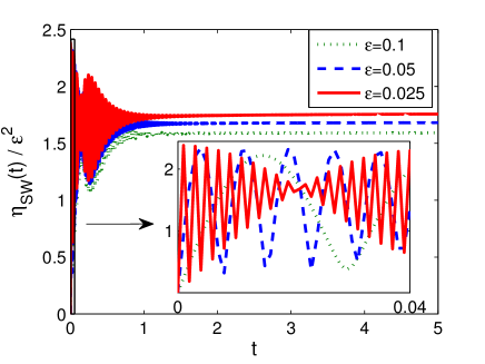
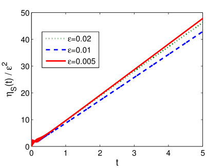
Figure 3: Time evolution of $\eta_{\rm sw}(t)$ and $\eta_{\rm s}(t)$ for the smooth initial data (6.1) under different $\varepsilon$.

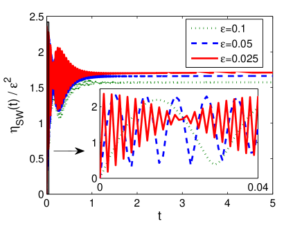
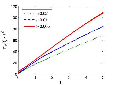
Figure 4: Time evolution of $\eta_{\rm sw}(t)$ and $\eta_{\rm s}(t)$ with nonsmooth data (6.2) for $m=2$ under different $\varepsilon$.

Figure 5: Time evolution of $\eta_{\rm sw}(t)$ and $\eta_{\rm s}(t)$ with nonsmooth data (6.2) for $m=1$ under different $\varepsilon$.

From Figs. 3-5, we can draw the following conclusions:

(i) The solution of the NKGE (1.1) converges to that of the NLSW (1.5) quadratically in $\varepsilon$ (and uniformly in time) provided that the initial data in (1.1) is smooth or at least satisfies $\phi_{1}$ and $\phi_{2}\in H^{2}(\Omega)$, i.e.

$$\|u(\cdot,t)-u_{\rm sw}(\cdot,t)\|_{H^{1}}\leq C_{0}\varepsilon^{2},\qquad t\geq 0,$$

where the constant $C_{0}>0$ is independent of $\varepsilon$ and time $t\geq 0$.

(ii) The solution of the NKGE (1.1) converges to that of the NLSE (1.6) quadratically in $\varepsilon$ (in general, not uniformly in time) provided that the initial data in (1.1) is smooth or at least satisfies $\phi_{1}$ and $\phi_{2}\in H^{3}(\Omega)$, i.e.

$$\|u(\cdot,t)-u_{\rm s}(\cdot,t)\|_{H^{1}}\leq(C_{1}+C_{2}T)\varepsilon^{2},\quad 0\leq t\leq T,$$

where $C_{1}$ and $C_{2}$ are two positive constants which are independent of $\varepsilon$ and $T$. On the contrary, if the regularity of the initial data is weaker, e.g. $\phi_{1}$ and/or $\phi_{2}\in H^{2}(\Omega)$, then the convergence rate collapses to linear rate, i.e.

$$\|u(\cdot,t)-u_{\rm s}(\cdot,t)\|_{H^{1}}\leq(C_{3}+C_{4}T)\varepsilon,\ \ 0\leq t\leq T,$$

where $C_{3}$ and $C_{4}$ are two positive constants which are independent of $\varepsilon$ and $T$. Rigorous mathematical justification for these numerical observations is on-going.

(iii) Under the same $\varepsilon$ and at the same time $t$, the error $\eta_{\rm sw}(t)$ is much small than $\eta_{\rm w}(t)$. It indicates that the NLSW (1.5) would be a better choice to design the LI scheme than the limit model (1.6), especially considering the long time behavior of the approximation.

6.2 Wave interactions in 2D

We take $d=2$ and $\lambda=1$ in the NKGE (1.1) and choose the initial data as

$$\begin{split}&\phi_{1}(x,y)=\exp{(-(x+2)^{2}-y^{2})}+\exp{(-(x-2)^{2}-y^{2})},\\ &\phi_{2}(x,y)=\exp{(-x^{2}-y^{2})},\qquad(x,y)\in{\mathbb{R}}^{2}.\end{split}$$ (6.4)

The problem is solved numerically on a bounded computational domain $\Omega=(-16,16)\times(-16,16)$ with the periodic boundary condition. Fig. 6 shows contour plots of the solutions of the NKGE (1.1) in 2D under different $\varepsilon$.

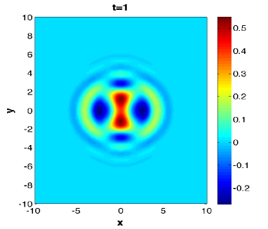
Figure 6: Contour plots of the solutions of the NKGE (1.1) in 2D at different time $t$ under $\varepsilon=0.05$ (first row) and $\varepsilon=0.005$ (second row).

7 Conclusions

We systematically studied and compared different numerical methods to solve the nonlinear Klein-Gordon equation (NKGE) in the nonrelativistic limit regime, while the solution is highly oscillatory in time in the limit regime. The numerical methods considered here include the classical finite difference time domain methods, the exponential wave integrator (EWI) spectral method, the time-splitting (TS) spectral method, the limit integrators, and the recently proposed uniformly accurate (UA) methods namely the multiscale time integrator (MTI) spectral method, the two-scale formulation (TSF) method and the iterative exponential integrator (IEI). We emphasized the finite time error bound of each method and the resolution capacity in terms of the oscillation wavelength in the limit regime. Systematical comparisons between the methods in the accuracy, computational complexity and other mathematical properties were carried out. Numerical experiments were done to show and compare the performance of each method from the classical regime to the limit regime. Our results show the EWI and TS methods are most efficient in the classical regime, while the UA methods are more powerful in the intermediate and limit regimes. Among the UA methods, the uniformly and optimally accurate methods are the most efficient and accurate for $\varepsilon\in(0,1]$ . Finally, the UA numerical methods were applied to study numerically the convergence rates of the NKGE (1.1) to its limiting models and to simulate wave interaction in two dimensions.

References

- [1] G. Adomian, Nonlinear Klein-Gordon equation, Appl. Math. Lett. 9 (1996) pp. 9-10.
- [2] X. Antoine, W. Bao and C. Besse Computational methods for the dynamics of the nonlinear Schrödinger/Gross-Pitaevskii equations, Comput. Phys. Commun. 184 (2013) pp. 2621-2633
- [3] D.D. Baǐnov and E. Minchev, Nonexistence of global solutions of the initial-boundary value problem for the nonlinear Klein-Gordon equation, J. Math. Phys. 36 (1995) pp. 756-762.
- [4] W. Bao and Y. Cai, Uniform error estimates of finite difference methods for the nonlinear Schrödinger equation with wave operator, SIAM J. Numer. Anal. 50 (2012) pp. 492-521.
- [5] W. Bao and Y. Cai, Mathematical theory and numerical methods for Bose-Einstein condensation, Kinet. Relat. Mod. 6 (2013) pp. 1-135
- [6] W. Bao and Y. Cai, Uniform and optimal error estimates of an exponential wave integrator sine pseudospectral method for the nonlinear Schrödinger equation with wave operator, SIAM J. Numer. Anal. 52 (2014) pp. 1103-1127.
- [7] W. Bao, Y. Cai, X. Jia and Q. Tang, A uniformly accurate multiscale time integrator pseudospectral method for the Dirac equation in the nonrelativistic limit regime, SIAM J. Numer. Anal. 54 (2016) pp. 1785-1812.
- [8] W. Bao, Y. Cai, X. Jia and Q. Tang, Numerical methods and comparison for the Dirac equation in the nonrelativistic limit regime, J. Sci. Comput. 71 (2017) pp. 1094-1134.
- [9] W. Bao, Y. Cai, X. Jia and J. Yin, Error estimates of numerical methods for the nonlinear Dirac equation in the nonrelativistic limit regime, Sci. China Math. 59 (2016) pp. 1461-1494.
- [10] W. Bao, Y. Cai and X. Zhao, A uniformly accurate multiscale time integrator pseudospectral method for the Klein-Gordon equation in the nonrelativistic limit regime, SIAM J. Numer. Anal. 52 (2014) pp. 2488-2511.
- [11] W. Bao and X. Dong, Analysis and comparison of numerical methods for the Klein-Gordon equation in the nonrelativistic limit regime, Numer. Math. 120 (2012) pp. 189-229.
- [12] W. Bao, X. Dong and X. Zhao, An exponential wave integrator pseudospectral method for the Klein-Gordon-Zakharov system, SIAM J. Sci. Comput. 35 (2013) pp. A2903-A2927.
- [13] W. Bao, X. Dong and X. Zhao, Uniformly accurate multiscale time integrators for highly oscillatory second order differential equations, J. Math. Study 47 (2014) pp. 111-150.
- [14] W. Bao, D. Jaksch and P.A. Markowich, Numerical solution of the Gross-Pitaevskii equation for Bose-Einstein condensation, J. Comput. Phys. 187 (2003) pp. 318-342.
- [15] W. Bao, S. Jin and P.A. Markowich, Numerical study of time-splitting spectral discretizations of nonlinear Schrödinger equations in the semi-classical regimes, SIAM J. Sci. Comput. 25 (2003) pp. 27-64.
- [16] W. Bao and L. Yang, Efficient and accurate numerical methods for the Klein-Gordon-Schrödinger equations, J. Comput. Phys. 225 (2007) pp. 1863-1893.
- [17] W. Bao and X. Zhao, A uniformly accurate multiscale time integrator pseudospectral method for the Klein-Gordon-Zakharov system in the high-plasma-frequency limit regime, J. Comput. Phys. 327 (2016) pp. 270-293.
- [18] W. Bao and X. Zhao, A uniformly accurate (UA) multiscale time integrator Fourier pseoduspectral method for the Klein-Gordon-Schrödinger equations in the nonrelativistic limit regime, Numer. Math. 135 (2017), pp. 833-873.
- [19] W. Bao and X. Zhao, A uniform second-order in time multiscale time integrator for the nonlinear Klein-Gordon equation in the nonrelativistic limit regime, preprint.
- [20] S. Baumstark, E. Faou and K. Schratz Uniformly accurate exponential-type integrators for Klein-Gordon equations with asymptotic convergence to classical splitting schemes in the NLS splitting, Math. Comp. 87 (2018) pp. 1227-1254.
- [21] P.M. Bellan, Fundamentals of Plasma Physics, Cambridge University Press, 2014.
- [22] A.G. Bratsos, On the numerical solution of the Klein-Gordon equation, Numer. Methods Partial Differ. Equ. 25 (2009) pp. 939-951.
- [23] P. Brenner and W. van Wahl, Global classical solutions of nonlinear wave equations, Math. Z. 176 (1981) pp. 87-121.
- [24] F.E. Browder, On nonlinear wave equations, Math. Z. 80 (1962) pp. 249-264.
- [25] W. Cao and B. Guo, Fourier collocation method for solving nonlinear Klein-Gordon equation, J. Comput. Phys. 108 (1993) pp. 296-305.
- [26] Ph. Chartier, N. Crouseilles, M. Lemou and F. Méhats, Uniformly accurate numerical schemes for highly oscillatory Klein-Gordon and nonlinear Schrödinger equations, Numer. Math. 129 (2015) pp. 211-250.
- [27] Ph. Chartier, N. Crouseilles, M. Lemou, F. Méhats and X. Zhao, Uniformly accurate methods for Vlasov equations with non-homogeneous strong magnetic field, Math. Comp. to appear.
- [28] Ph. Chartier, M. Lemou, F. Méhats and G. Vilmart, A new class of uniformly accurate methods for highly oscillatory evolution equations, Found. Comput. Math. to appear.
- [29] Ph. Chartier, F. Méhats, M. Thalhammer and Y. Zhang, Improved error estimates for splitting methods applied to highly-oscillatory nonlinear Schrödinger equations, Math. Comp. 85 (2016), pp. 2863-2885.
- [30] P.A. Clarkson, J.B. McLeod, P.J. Olver and R. Ramani, Integrability of Klein-Gordon equations, SIAM J. Math. Anal. 17 (1986) pp. 798-802.
- [31] D. Cohen, E. Hairer and Ch. Lubich, Conservation of energy, momentum and actions in numerical discretizations of nonlinear wave equations, Numer. Math. 110 (2008) pp. 113-143.
- [32] D. Cohen, E. Hairer and Ch. Lubich, Modulated Fourier expansions of highly oscillatory differential equations, Found. Comput. Math. 3 (2003) pp. 327-345.
- [33] N. Crouseilles, M. Lemou, F. Méhats and X. Zhao, Uniformly accurate forward semi-Lagrangian methods for highly oscillatory Vlasov-Poisson equations, SIAM J. Multiscale Model. Simul. 15 (2017) pp. 723-744.
- [34] N. Crouseilles, M. Lemou, F. Méhats and X. Zhao, Uniformly accurate Particle-in-Cell method for the long time two-dimensional Vlasov-Poisson equation with uniform strong magnetic field, J. Comput. Phys. 346 (2017) pp. 172-190.
- [35] A.S. Davydov, Quantum Mechanics, 2nd edn. Pergamon, Oxford (1976).
- [36] E.Y. Deeba and S.A. Khuri, A decomposition method for solving the nonlinear Klein-Gordon equation, J. Comput. Phys. 124 (1996) pp. 442-448.
- [37] M. Dehghan and A. Shokri, Numerical solution of the nonlinear Klein-Gordon equation using radial basis functions, J. Comput. Appl. Math. 230 (2009) pp. 400-410.
- [38] R.O. Dendy, Plasma Dynamics, Oxford University Press, 1990.
- [39] P. Deuflhard, A study of extrapolation methods based on multistep schemes without parasitic solutions, ZAMP. 30 (1979) pp. 177-189.
- [40] X. Dong, Z. Xu and X. Zhao, On time-splitting pseudospectral discretization for nonlinear Klein-Gordon equation in nonrelativistic limit regime, Commun. Comput. Phys. 16 (2014) pp. 440-66.
- [41] D.B. Duncan, Symplectic finite difference approximations of the nonlinear Klein-Gordon equation, SIAM J. Numer. Anal. 34 (1997) pp.1742-1760.
- [42] E. Faou and K. Schratz, Asympotic preserving schemes for the Klein-Gordon equation in the non-relativistic limit regime, Numer. Math. 126 (2014) pp. 441-469.
- [43] L. Gauckler, E. Hairer and Ch. Lubich, Dynamics, numerical analysis, and some geometry, Proc. Int. Cong. Math. 1 (2018) pp. 453-486.
- [44] W. Gautschi, Numerical integration of ordinary differential equations based on trigonometric polynomials, Numer. Math. 3 (1961) pp. 381-397.
- [45] J. Ginibre and G. Velo, The global Cauchy problem for the nonlinear Klein-Gordon equation, Math. Z. 189 (1985) pp. 487-505.
- [46] J. Ginibre and G. Velo, The global Cauchy problem for the nonlinear Klein-Gordon equation–II, Ann. Inst. H. Poincaré Anal. Non Linéaire 6 (1989) pp. 15-35.
- [47] V. Grimm, On error bounds for the Gautschi-type exponential integrator applied to oscillatory second-order differential equations, Numer. Math. 100 (2005) pp. 71-89.
- [48] V. Grimm, A note on the Gautschi-type method for oscillatory second-order differential equations, Numer. Math. 102 (2005) pp. 61-66.
- [49] A.M. Grundland and E. Infeld, A family of nonlinear Klein-Gordon equations and their solutions, J. Math. Phys. 33 (1992) pp. 2498-2503.
- [50] E. Hairer, Ch. Lubich and G. Wanner, Geometric Numerical Integration: Structure-Preserving Algorithms for Ordinary Differential Equations, Springer, Berlin, 2006.
- [51] M. Hochbruck and Ch. Lubich, A Gautschi-type method for oscillatory second-order differential equations, Numer. Math. 83 (1999) pp. 402-426.
- [52] M. Hochbruck and A. Ostermann, Exponential integrators, Acta Numer. 19 (2010) pp. 209-286.
- [53] K. Huang, C. Xiong and X. Zhao, Scalar-field theory of dark matter, Inter. J. Modern Physics A 29 (2014) article 1450074.
- [54] S. Ibrahim, M. Majdoub and N. Masmoudi, Global solutions for a semilinear, two-dimensional Klein-Gordon equation with exponential-type nonlinearity, Comm. Pure Appl. Math. 59 (2006) pp. 1639-1658.
- [55] S. Jiménez and L. Vázquez, Analysis of four numerical schemes for a nonlinear Klein-Gordon equation, Appl. Math. Comput. 35 (1990) pp. 61-94.
- [56] M.E. Khalifa and M. Elgamal, A numerical solution to Klein-Gordon equation with Dirichlet boundary condition, Appl. Math. Comput. 160 (2005), pp. 451-475.
- [57] H.J. Landau, Necessary density conditions for sampling and interpolation of certain entire functions, Acta Math. 117 (1967) pp. 37–52.
- [58] X. Li and B. Guo, A Legendre spectral method for solving the nonlinear Klein-Gordon equation, J. Comput. Math. 15 (1997) pp. 105–126.
- [59] S. Li and L. Vu-Quoc, Finite difference calculus invariant structure of a class of algorithms for the nonlinear Klein-Gordon equation, SIAM J. Numer. Anal. 32 (1995) pp. 1839-1875.
- [60] C. Liu, A. Iserles and X. Wu, Symmetric and arbitrarily high-order Birkhoff-Hermite time integrators and their long-time behaviour for solving nonlinear Klein-Gordon equations, J. Comp. Phys. 356 (2018), pp. 1-30.
- [61] S. Machihara, K. Nakanishi and T. Ozawa, Nonrelativistic limit in the energy space for nonlinear Klein-Gordon equations, Math. Ann. 322 (2002) pp. 603-621.
- [62] N. Masmoudi and K. Nakanishi, From nonlinear Klein-Gordon equation to a system of coupled nonlinear Schrödinger equations, Math. Ann. 324 (2002) pp. 359-389.
- [63] R.I. McLachlan and G.R.W. Quispel, Splitting methods, Acta Numer. 11 (2002) pp. 341-434.
- [64] C. Morawetz and W. Strauss, Decay and scattering of solutions of a nonlinear relativistic wave equation, Comm. Pure Appl. Math. 25 (1972) pp. 1-31.
- [65] B. Najman, The nonrelativistic limit of the nonlinear Klein-Gordon equation, Nonlinear Anal. 15 (1990) pp. 217-228.
- [66] A. Ostermann and K. Schratz, Low regularity exponential-type integrators for semilinear Schrödinger equations in the energy space, Found. Comput. Math. 18 (2018) pp. 731-755.
- [67] K. Schratz and X. Zhao, On the comparison of asymptotic expansion techniques for the nonlinear Klein-Gordon equation in the nonrelativistic limit regime, preprint (2019).
- [68] C.E. Shannon, A mathematical theory of communication, Bell System Technical Journal, 27 (1948) pp. 379-423.
- [69] C.E. Shannon, A mathematical theory of communication, Bell System Technical Journal, 27 (1948) pp. 623-666.
- [70] C. E. Shannon, Communication in the presence of noise, Proceedings of the Institute of Radio Engineers, 37 (1949) 10–21.
- [71] J. Shen, T. Tang and L. Wang, Spectral Methods: Algorithms, Analysis and Applications, Springer, 2011.
- [72] W. Strauss and L. Vázquez, Numerical solution of a nonlinear Klein-Gordon equation, J. Comput. Phys. 28 (1978) pp. 271-278.
- [73] Y. Tourigny, Product approximation for nonlinear Klein-Gordon equations, IMA J. Numer. Anal. 9 (1990) pp. 449-462.
- [74] Y. Wang and X. Zhao, Symmetric high order Gautschi-type exponential wave integrators pseudospectral method for the nonlinear Klein-Gordon equation in the nonrelativistic limit regime, Int. J. Numer. Anal. Model. 15 (2018) pp. 405-427.
- [75] C. Xiong, M.R.R. Good, Y. Guo, X. Liu and K. Huang, Relativistic superfluidity and vorticity from the nonlinear Klein-Gordon equation, Phys. Rev. D 90 (2014) article 125019.
- [76] X. Zhao, A combination of multiscale time integrator and two-scale formulation for the nonlinear Schrödinger equation with wave operator, J. Comput. Appl. Math. 326 (2017) pp. 320-336.