Detecting the Presence of ENF Signal in Digital Videos: a Superpixel based Approach

Abstract

ENF (Electrical Network Frequency) instantaneously fluctuates around its nominal value (50/60 Hz) due to a continuous disparity between generated power and consumed power. Consequently, luminous intensity of a mains-powered light source varies depending on ENF fluctuations in the grid network. Variations in the luminance over time can be captured from video recordings and ENF can be estimated through content analysis of these recordings. In ENF based video forensics, it is critical to check whether a given video file is appropriate for this type of analysis. That is, if ENF signal is not present in a given video, it would be useless to apply ENF based forensic analysis. In this work, an ENF signal presence detection method is introduced for videos. The proposed method is based on multiple ENF signal estimations from steady superpixels, i.e. pixels that are most likely uniform in color, brightness, and texture, and intra-class similarity of the estimated signals. Subsequently, consistency among these estimates is then used to determine the presence or absence of an ENF signal in a given video. The proposed technique can operate on video clips as short as 2 minutes and is independent of the camera sensor type, i.e. CCD or CMOS.

I Introduction

ENF (Electrical Network Frequency) is a time varying signal fluctuating continuously around its nominal value (50/60 Hz) due to the instantaneous imbalance between power consumption and power generation [1]. For each time instance, ENF fluctuation is almost the same across the entire interconnected power grid network [2]. Accordingly, electric frequency measured at any location connected to a particular mains power can be used as a reference ENF signal for the whole area covered by that power network for the relevant time period [3]. This property of electric frequency, as well as the ability to extract it from multimedia files, has led to the exploitation of ENF in digital media forensics in recent years. It can be used for a variety of forensic and anti-forensic applications including audio/video authentication [4, 5], [6], time stamp verification [7, 8, 9], and power grid identification [10].

An ENF signal is embedded in audio recordings made in settings where the electromagnetic field or acoustic mains hum exists and it can be estimated from these recordings with time-domain or frequency-domain approaches [2], [7], [11], [12], [13]. Recently, it was found that ENF can also be estimated from video captured under illumination of a light source powered by mains grid [3]. The intensity of illumination from any light source connected to the mains power varies depending on ENF variations in the grid network. Although the human eye cannot perceive, ENF can be estimated by analysis of subtle illumination variations in steady content along subsequent video frames.

Two different ENF estimation methods for ENF based forensic analysis of digital video have been proposed in the literature: a method tailored to videos recorded by CCD sensor [3] and a technique for videos captured by CMOS sensor [3, 9, 14]. While the former is based on averaging all the steady pixels in each frame along the video, the latter processes steady pixels based on a rolling shutter sampling mechanism [14], [15], [16], [17].

In ENF based video forensics, it is important to test whether a video contains any traces of ENF before moving on to further analysis. For instance, if a video does not contain any ENF signal it would be useless to search in existing ENF databases for video time-stamp or region-of-recording verification. More importantly, a substantial amount of computational load and time can be saved if a quick test can establish the absence of an ENF signal. To the best of our knowledge, none of the work in the literature presents an approach that can automatically detect the presence of an ENF signal in a video regardless of the imaging sensor type, e.g. CCD or CMOS.

In this letter, a superpixel based ENF signal presence detection technique is proposed. The proposed method performs multiple “so-called ENF” signal estimations from different steady object regions having very close reflectance properties, i.e. superpixels [18]. Our motivation to use superpixels is that each pixel in a superpixel region is almost uniform in brightness, color and texture, and hence has uniform reflectance characteristics. Working on such a region provides the possibility of estimating ENF from videos taken by not only CCD camera but also by CMOS camera, which uses rolling shutter mechanism. In the proposed algorithm, a “so-called ENF signal” is estimated from each steady superpixel separately. The reason we use the term “so-called ENF” is because the estimated signal is initially unknown to be actually an ENF signal. Depending on the similarity of the estimated signals from each steady superpixel, it can be decided whether any ENF signal is present in the test video or not. It should be noted that the proposed method does not require any verification against a reference ENF database.

II ENF Power Model

Instantaneous power grid voltage can be modeled as follows:

$$\begin{split}V(t)&={\color[rgb]{0,0,0}\sqrt{2}V_{0}\cos(\phi(t))}\\ &=\sqrt{2}V_{0}\cos(2\pi f_{n}t+\theta(t)+{\color[rgb]{0,0,0}\alpha})\\ &=\sqrt{2}V_{0}\cos(2\pi f_{n}t+2\pi\int_{0}^{t}{f_{e}(\tau)\mathrm{d}\tau}+{\color[rgb]{0,0,0}\alpha})\\ \end{split}$$ (1)

where $f_{n}$ is nominal frequency (50/60Hz), $V_{0}$ is effective mains voltage and $\alpha$ is initial phase offset [1]. $f_{e}(t)$ represents instantaneous fluctuations from nominal frequency and $\theta(t)$ denotes instantaneous phase which varies depending on supply-demand power imbalance. From the above equations, the instantaneous mains power frequency at time $t$ can be expressed as

$$\begin{split}f(t)&=\frac{1}{2\pi}\frac{d{\color[rgb]{0,0,0}\phi(t)}}{dt}=f_{n}+f_{e}(t)\\ \end{split}$$ (2)

As $f_{n}$ is constant, electric network frequency alters depending on $f_{e}(t)$ variations. By benefiting from the model in [1], $f_{e}(t)$ can be written as

$$f_{e}(t)=\frac{f_{n}}{2H}(P_{s}(t)-P_{d}(t))$$ (3)

where $P_{s}(t)$ denotes supplied power, $P_{d}(t)$ is total demanded power with losses and $H$ represents an inertia constant. Accordingly, for each time instance, $f_{e}(t)$ and $f(t)$ change depending on the instantaneous difference between generated and consumed power.

III ENF Estimation from Video

III-A Light Source Flicker and ENF

Intensity of illumination from any light source connected to the mains power varies depending on ENF variations in grid network. As light source flickers at both the positive and negative cycles of AC current, the illumination frequency becomes double the mains power frequency. Accordingly, the illumination signal can be treated as the absolute form of the cosine function in $(\ref{Eq_PowerGridVoltage})$. For example in Europe, nominal ENF in any region is 50 Hz, thus frequency of illumination varies around 100 Hz. According to the Nyquist Sampling Theorem, a sampling rate of at least 200 Hz is needed in order to extract illumination frequency accurately from sampled data. Although most consumer cameras are unable to provide such high frame sampling rates, it is still possible to estimate illumination frequency from its alias frequency. Let $f_{s}$ be the camcorder sampling frequency and $f_{l}$ be the frequency of light source illumination. Then $f_{a}$ the aliased frequency of illumination is obtained as follows [19]:

$$f_{a}=\mathinner{\!\left\lvert f_{l}-k\cdot f_{s}\right\rvert}<\frac{f_{s}}{2},\quad\exists k\in\mathbb{{\color[rgb]{0,0,0}N}}$$ (4)

Accordingly, when a light source illumination signal in 100 Hz is sampled with 29.97 fps camera, the base alias frequency of ENF is obtained as 10.09 Hz.

III-B Superpixel based ENF Estimation

Figure 1: A sample image with superpixels.

In this section, a superpixel based ENF estimation method for video is proposed. Unlike available methods in the literature [3], [9], we propose to estimate ENF from only steady superpixels, rather than all steady pixels along video frames. The SLIC (Simple Linear Iterative Clustering) segmentation algorithm [18] is used to compute superpixel regions in the experiments. A sample image segmented with the SLIC algorithm and its superpixels is given in Fig. 1. The underlying idea of the proposed ENF estimation is that each pixel in a superpixel region/set is assumed to have uniform reflectance characteristics.

The amount of illumination at any pair of pixel coordinates $x,y$, received by a camera at any moment $n$ can be written as [20]:

$$I(x,y,n)=i_{s}(x,y,n)\cdot r(x,y)$$ (5)

where $r(x,y)$ denotes the amount of reflected illumination and $i_{s}(x,y,n)$ is instantaneous light source illumination. For a point light source, $i_{s}(x,y,n)$ can be expressed in terms of mains electricity voltage approximately as:

$${\color[rgb]{0,0,0}i_{s}(x,y,n)\approx\frac{\beta}{d_{s}(x,y)^{2}}\cdot\mathinner{\!\left\lvert V(n)\right\rvert}}$$ (6)

where $\beta$ is a transform factor for voltage to luminance conversion and $d_{s}(x,y)$ is the distance between the spatial position $(x,y)$ and the light source. The reason $V(n)$ is in absolute form is that light source produces illumination in both positive and negative cycles of electrical power grid voltage. In a superpixel region, the reflectance factor $r(x,y)$ can be assumed to be constant. Similarly, the distance of any pixel in a superpixel $S$ to the light source $d_{s}(x,y)$ can be considered constant as well. Thus, for $k$th steady superpixel $S_{k}$, $(\ref{eqI_1})$ can be rewritten in the following form:

$${\color[rgb]{0,0,0}I_{k}(x,y,n)\approx\beta\cdot\frac{r_{k}}{d_{k}^{2}}\cdot\mathinner{\!\left\lvert V(n)\right\rvert}\text{ , }(x,y)\in{S_{k}}}$$ (7)

where $r_{k}$ denotes a constant reflectance factor for pixels belonging to $k$th steady superpixel region ($S_{k}$), $k\in\{1,...,L\}$. $L$ is the number of steady superpixels, $d_{k}$ is the approximate distance of superpixel $S_{k}$ to the light source. As it can be seen from $(\ref{eqI_2})$, $I_{k}(x,y,n)$ is directly proportional to $V(n)$, which means that the frequency of power grid voltage $V(n)$ can be directly estimated from $I_{k}(x,y,n)$. Illumination variations at any superpixel region $S$ can be estimated by averaging the steady pixels in $S$, resulting in $L$ illumination vectors. From each of the illumination vectors, ENF variations can be estimated using any of the frequency or time domain approaches discussed in [9], [11]. In this paper, ENF is estimated from local intensity variations using STFT (Short Time Fourier Transform) and quadratic interpolation. In order to compute STFT we have used 20 sec. time windows with 19 sec. overlapping resulting 1-second temporal ENF resolution [21]. It is important to note the content of the superpixel region should be unchanged all along the consecutive video frames, in order to estimate ENF successfully. This will be addressed in the next section.

IV Detection of ENF Signal Presence

In this section, a superpixel based ENF presence detector for digital video files is presented based on multiple ENF signal estimations from steady superpixel regions. The main steps of the proposed technique are illustrated in Table I. According to the table, one frame, e.g. the middle frame $\mathbb{F}_{r}$, in a selected video shot $C$ is segmented into regions having similar pixel characteristics, i.e. superpixels. Then, within each superpixel region, the points that are steady throughout all frames, i.e. non-moving pixels are located. Superpixels having a low number of steady pixels ($m_{l}<\tau$) are not used in ENF estimation. In this study, the value of $\tau$ has been determined empirically as 30$\times$30 pixels. For each steady superpixel $S_{k}$ and each video frame $\mathbb{F}_{n}$, the average intensity $Y_{k}(n)$ is computed from steady pixels of region $S_{k}$. From each intensity variation vector $\mathbb{Y}_{k}$, a “so-called” ENF vector $\mathbb{E}_{k}$ is estimated along all the subsequent video frames of the given shot. As stated in introduction, the reason we use the prefix “so-called’ is that it is initially unknown to be actually ENF or not.

Next, the similarity of estimated ENF vectors is analyzed to decide whether ENF signal is present or not in the test video. For this purpose, a representative ENF vector $\mathbb{E}_{r}$ is computed by means of element-wise mean or median operation of all the estimated ENF vectors. Next, Pearson correlation coefficients between each estimated $\mathbb{E}_{k}$ and the representative vector $\mathbb{E}_{r}$ are calculated as follows:

$$\begin{split}\rho(k)&=\textrm{corr}(\mathbb{E}_{k},\,\mathbb{E}_{r})=\frac{<\mathbb{E}_{k}-\bar{\mathbb{E}}_{k},\,\mathbb{E}_{r}-\bar{\mathbb{E}}_{r}>}{\parallel\mathbb{E}_{k}-\bar{\mathbb{E}}_{k}\parallel\,\parallel\mathbb{E}_{r}-\bar{\mathbb{E}}_{r}\parallel}\\ \end{split}$$ (8)

where $\parallel\cdot\parallel$ denotes $L_{2}$ (Euclidean) norm and $<\cdot>$ is the dot product. The sample mean is denoted with overline. Afterwards, a decision metric is computed based on the following operations: $f_{1}=\textrm{max}({\boldsymbol{\rho}})$,   $f_{2}=\textrm{mean}(\boldsymbol{\rho})$,   $f_{3}=\textrm{median}(\boldsymbol{\rho})$,   $f_{4}=\textrm{corr}(\mathbb{E}_{i},\,\mathbb{E}_{j})$, where $\mathbb{E}_{i}$ and $\mathbb{E}_{j}$ are the vectors yielding the greatest $\rho$ values (top two closest vectors to $\mathbb{E_{r}}$). If the decision metric is greater than a predefined decision threshold value, the video is labeled as having an ENF signal.

TABLE I: Algorithm: Detection of ENF Signal Presence

Step	Description
1	Pick any video shot $C$. Let $\mathbb{F}_{n}$ be the $n$th frame in $C$, where $n\in\{1,...,N\}$.
2	Let the middle frame $\mathbb{F}_{r}$ be the representative frame in $C$, where $r=\lfloor N/2\rfloor$.
3	Compute superpixel regions for the representative frame. Let $\Omega_{l}$ be the $l$th superpixel in $\mathbb{F}_{r}$, $l\in\{1,...,{\color[rgb]{0,0,0}P}\}$. ${\color[rgb]{0,0,0}P}$ is the total number of the superpixels.
4	Let $\Phi$ be the set of all steady pixels in which the video content do not change with time in $\mathbb{F}_{r}$.
5	Compute the number of steady pixels $m_{l}$ in each $\Omega_{l}$ using the steady pixel set $\Phi$.
6	Compute steady superpixel set $S$ from $\{\Omega_{l}\}$: $S=\{\Omega_{l}\mid m_{l}>\tau\}$, where $\tau$ is a pre-defined threshold for the minimum number of non-changing pixels in a superpixel region.
7	For each steady superpixel $S_{k}$ and each frame $\mathbb{F}_{n}$, compute the average intensity $Y_{k}(n)$, only from steady pixels of region $S_{k}$. $k\in\{1,...,L\}$, and $L$ is the total number of steady superpixels.
8	Estimate ENF variation signal $\mathbb{E}_{k}$ from local intensity variations $\mathbb{Y}_{k}$ for each superpixel $S_{k}$.
9	Place all $E_{k}(i)$ into a matrix $\mathbb{M}$ such that $M(k,i)=E_{k}(i)$, where $i\in\{1,...,t\}$ and $t$ is the ENF vector length. Let $\mathbb{E}_{r}$ be the representative ENF vector computed by means of element-wise median or mean operation of all $\mathbb{E}_{k}$ vectors, where $n$th sample of $\mathbb{E}_{r}$ is computed as:
	$E_{r}(i|\text{mean})=\underset{k}{\mathrm{mean}}\{M(k,i)\}$
	$E_{r}(i|\text{median})=\underset{k}{\mathrm{median}}\{M(k,i)\}$
10	Compute similarity of each $\mathbb{E}_{k}$ with $\mathbb{E}_{r}$ by Pearson correlation, $\rho(k)$.
11	Compute mean, median, maximum, and similar statistics of $\boldsymbol{\rho}$ vector as decision metrics.
12	If the computed metric is greater than a predefined decision threshold, the presence of ENF signal in the video is confirmed.

V Experiments and Results

V-A Experimental Setup

In this section, the performance of the proposed method is evaluated by conducting experiments on partially-moving-content videos captured in various indoor and outdoor settings in Turkey, where nominal ENF frequency is 50 Hz. ENF signal presence was searched in a total of 160 videos, one half of which were recorded by PowerShot SX230HS (CMOS sensor) and the other half were recorded by Canon PowerShot SX210IS (CCD sensor). For CMOS, the Canon PowerShot SX230HS model camcorder was intentionally picked as it has been used in most ENF related works [9], [14], [15] and [17]. The CCD equivalent of the same camera brand and model was picked so as to do a fair comparison of the algorithm according to the sensor type. Out of 80 videos for each sensor-camera type, one-quarter was captured at night under illumination of various mains-powered light sources such as LED, fluorescent tube, CFL, tungsten halogen, sodium-vapor lamp, street light. A second quarter were recorded under illumination of mains-powered light sources but in daylight settings such as in a room with an opened window or next to a lamp on the balcony in the sunset afternoon. The third quarter were taken under illumination of non-mains-powered light sources in daylight settings and the last quarter were captured at night under illumination of non-mains-powered light sources such as moonlight, vehicle headlight, candle, projector torch, smart-phone torch and laptop screen. Hence, each video is initially known to contain an ENF signal or not. All the videos were created in 640$\times$480 resolution with a sampling frequency of 29.97 fps. The camera was fixed during recording and it was ensured that each video has some steady content in addition to moving content. When sampled with 29.97 fps, the peak alias of 100 Hz can be computed as 10.09 as discussed in section III-A. Therefore, 10.09 Hz frequency band was utilized for ENF signal estimation from the relevant video files. Although the videos were in a variety of lengths between 2 minutes and 15 minutes, a 2-minute clip of each video was used for ENF detection experiment. It is also notable that the representative frame for each video was segmented into about 48 superpixel regions, which corresponds to about 6400 ($80\times 80$) pixels per superpixel for a frame of 640$\times$480 pixels resolution.

Figure 2: ROC curves of ENF presence detection for videos recorded by both CCD and CMOS sensors, 160 videos. $\mathbb{E}_{r}$ computed with $\mathbb{mean}$ operation.

Figure 3: ROC curves of ENF presence detection for videos recorded by both CCD and CMOS sensors, 160 videos. $\mathbb{E}_{r}$ computed with the $\mathbb{median}$ operation.

V-B Experimental Results

TABLE II: ENF Detection Performance (AUC) based on Mean based Representative ENF

Sensor Type	# Videos	$f1$	$f2$	$f3$	$f4$
CCD	80	0.836	$\mathbb{\color[rgb]{1,0,0}0.896}$	0.895	0.813
CMOS	80	0.760	$\mathbb{\color[rgb]{1,0,0}0.883}$	0.866	0.700
Any (Mixed)	160	0.798	$\mathbb{\color[rgb]{1,0,0}0.886}$	0.881	0.761

TABLE III: ENF Detection Performance (AUC) based on Median based Representative ENF

Sensor Type	# Videos	$f1$	$f2$	$f3$	$f4$
CCD	80	$\mathbb{\color[rgb]{1,0,0}0.985}$	0.947	0.931	0.960
CMOS	80	$\mathbb{\color[rgb]{1,0,0}0.959}$	0.942	0.941	0.944
Any (Mixed)	160	$\mathbb{\color[rgb]{1,0,0}0.973}$	0.939	0.931	0.952

In this section, the accuracy of the proposed ENF detection algorithm is tested on the video dataset described in Section V-A by computation of a Receiver Operating Characteristics (ROC) curve and area under the curve (AUC). For this purpose, the following binary hypotheses are defined:
$H_{0}\mathrel{\mathop{\ordinarycolon}}$ The video does not contain ENF signal
$H_{1}\mathrel{\mathop{\ordinarycolon}}$ The video contains ENF signal
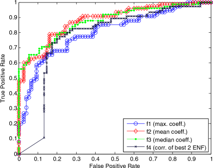
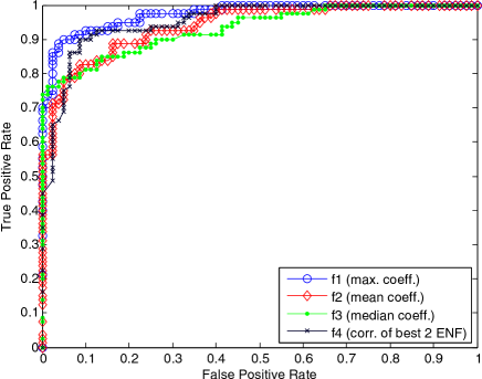
Under these hypotheses, $f_{1}$, $f_{2}$, $f_{3}$ and $f_{4}$ decision metrics, introduced in Section IV, were computed for each video. Each decision metric was computed with the use of both mean-based representative ENF and median-based representative ENF, respectively and was assigned to the corresponding hypothesis, $H_{0}$ or $H_{1}$. Fig. 2 provides ROC curves obtained for decision metrics which are formed via mean based representative ENF computation. Whereas Fig. 3 illustrates ROC curves obtained for decision metrics that are calculated based on the utilization of median based representative ENF. From the ROC curves in Fig. 2 and Fig. 3, a significant enhancement in the detection performance can explicitly be observed for all metrics when the decision metrics are formed with the use of median-based representative ENF. Table II and III provides the area under the ROC curves (AUC) in Fig. 2 and Fig. 3, respectively as well as AUC values for each sensor type, separately. The computed AUC values in Table III are considerably higher not only for mixture of sensor types but also for each sensor type independently. According to the Fig. 3, the detection metric $f_{1}$ outperforms other metrics when testing a mixture video dataset whose source sensor type is unknown.

VI Discussion and Conclusion

In this paper, a superpixel based ENF detection algorithm for video is presented. The proposed method is able to work on short video clips of about 2 minutes-length and can be used to detect and differentiate the videos that are appropriate for ENF based forensic analysis from ENF free videos on a disk under investigation or in social media. By doing this, ENF free videos are not exposed unnecessarily to the execution of entire ENF based analysis; hence a substantial amount of time and computational load can be saved. The algorithm is able to operate independently of the source camera sensor type, CCD or CMOS and achieves a very high ENF signal presence detection accuracy for videos captured by both sensor types.

References

- [1] M. Bollen and I. Gu, Signal processing of power quality disturbances. Wiley-Interscience, 2006.
- [2] C. Grigoras, “Digital audio recording analysis–the electric network frequency criterion,” International Journal of Speech Language and the Law, vol. 12, no. 1, pp. 63–76, 2005.
- [3] R. Garg, A. Varna, and M. Wu, “Seeing ENF: natural time stamp for digital video via optical sensing and signal processing,” Proceedings of the 19th ACM international conference on Multimedia, pp. 23–32, 2011.
- [4] G. Hua, Y. Zhang, J. Goh, and V. L. L. Thing, “Audio authentication by exploring the absolute-error-map of ENF signals,” IEEE Transactions on Information Forensics and Security, vol. 11, no. 5, pp. 1003–1016, 2016.
- [5] M. Savari, A. W. Abdul Wahab, and N. B. Anuar, “High-performance combination method of electric network frequency and phase for audio forgery detection in battery-powered devices,” Forensic Science International, vol. 266, pp. 427–439, 2016.
- [6] W. H. Chuang, R. Garg, and M. Wu, “Anti-forensics and countermeasures of electrical network frequency analysis,” IEEE Transactions on Information Forensics and Security, vol. 8, no. 12, pp. 2073–2088, Dec 2013.
- [7] N. Fechner and M. Kirchner, “The humming hum: Background noise as a carrier of ENF artifacts in mobile device audio recordings,” Proceedings - 8th International Conference on IT Security Incident Management and IT Forensics, IMF 2014, pp. 3–13, 2014.
- [8] D. Bykhovsky and A. Cohen, “Electrical network frequency (ENF) maximum-likelihood estimation via a multitone harmonic model,” IEEE Transactions on Information Forensics and Security, vol. 8, no. 5, pp. 744–753, 2013.
- [9] R. Garg, A. L. Varna, A. Hajj-Ahmad, and M. Wu, “Seeing ENF: Power-signature-based timestamp for digital multimedia via optical sensing and signal processing,” IEEE Transactions on Information Forensics and Security, vol. 8, no. 9, pp. 1417–1432, 2013.
- [10] A. Hajj-Ahmad, R. Garg, and M. Wu, “ENF-based region-of-recording identification for media signals,” IEEE Transactions on Information Forensics and Security, vol. 6013, no. c, p. 1, 2015.
- [11] C. Grigoras, “Applications of ENF criterion in forensic audio, video, computer and telecommunication analysis,” Forensic Science International, vol. 167, no. 2-3, pp. 136–145, 2007.
- [12] C. Grigoras, A. Cooper, and M. Michalek, “Best practice guidelines for ENF analysis in forensic authentication of digital evidence,” Forensic Speech and Audio Analysis Working Group, no. 001, pp. 1–10, 2009.
- [13] J. Chai, F. Liu, Z. Yuan, R. Conners, and Y. Liu, “Source of ENF in battery-powered digital recordings,” Audio Engineering Society Convention 135, 2013.
- [14] A. Hajj-Ahmad, A. Berkovich, and M. Wu, “Exploiting power signatures for camera forensics,” IEEE Signal Processing Letters, vol. 23, no. 5, pp. 713–717, 2016.
- [15] H. Su, A. Hajj-Ahmad, C.-W. Wong, R. Garg, and M. Wu, “ENF signal induced by power grid: a new modality for video synchronization,” in Proceedings of the 2Nd ACM International Workshop on Immersive Media Experiences, 2014, pp. 13–18.
- [16] H. Su, A. Hajj-Ahmad, M. Wu, and D. W. Oard, “Exploring the use of ENF for multimedia synchronization,” ICASSP, IEEE International Conference on Acoustics, Speech and Signal Processing - Proceedings, pp. 4613–4617, 2014.
- [17] H. Su, A. Hajj-Ahmad, R. Garg, and M. Wu, “Exploiting rolling shutter for ENF signal extraction from video,” in 2014 IEEE International Conference on Image Processing (ICIP), 2014, pp. 5367–5371.
- [18] R. Achanta, A. Shaji, K. Smith, A. Lucchi, P. Fua, and S. Susstrunk, “SLIC superpixels,” EPFL Technical Report 149300, no. June, p. 15, 2010.
- [19] A. Hajj-Ahmad, S. Baudry, B. Chupeau, and G. Doërr, “Flicker forensics for pirate device identification,” Proceedings of the 3rd ACM Workshop on Information Hiding and Multimedia Security - IH&MMSec ’15, no. August, pp. 75–84, 2015.
- [20] R. C. Gonzalez and R. E. Woods, Digital Image Processing. Pearson Education, 2011.
- [21] A. Cooper, “The electric network frequency (ENF) as an aid to authenticating forensic digital audio recordings–an automated approach,” AES 33rd International Conference, pp. 1–10, 2008.