Data Poisoning against Differentially-Private Learners:
Attacks and Defenses

Abstract

Data poisoning attacks aim to manipulate the model produced by a learning algorithm by adversarially modifying the training set. We consider differential privacy as a defensive measure against this type of attack. We show that such learners are resistant to data poisoning attacks when the adversary is only able to poison a small number of items. However, this protection degrades as the adversary poisons more data. To illustrate, we design attack algorithms targeting objective and output perturbation learners, two standard approaches to differentially-private machine learning. Experiments show that our methods are effective when the attacker is allowed to poison sufficiently many training items.

1 Introduction

As machine learning is increasingly used for consequential decisions in the real world, the security concerns have received more and more scrutiny. Most machine learning systems were originally designed without much thought to security, but researchers have since identified several kinds of attacks under the umbrella of adversarial machine learning. The most well-known example is adversarial examples [19], where inputs are crafted to fool classifiers. More subtle methods aim to recover training examples [8], or even extract the model itself [20].

In data poisoning attacks [2, 11, 14, 1, 13, 21, 15, 9, 23, 22], the adversary corrupts examples at training time to manipulate the learned model. As is generally the case in adversarial machine learning, the rise of data poisoning attacks has outpaced the development of robust defenses. While attacks are often evaluated against specific target learning procedures, effective defenses should provide protection—ideally guaranteed—against a broad class of attacks. In this paper, we study differential privacy [7, 6] as a general defensive technique against data poisoning. While differential privacy was originally designed to formalize privacy—the output should not depend too much on any single individual’s private data—it also provides a defense against data poisoning. Concretely, we establish quantitative bounds on how much an adversary can change the distribution over learned models by manipulating a fixed number of training items. We are not the first to design defenses to data poisoning [18, 17], but our proposal has several notable strengths compared to previous work. First, our defense provides provable protection against a worst-case adversary. Second, our defense is general. Differentially-private learning procedures are known for a wide variety of tasks, and new algorithms are continually being proposed. These learners are all resilient against data poisoning.

We complement our theoretical bounds with an empirical evaluation of data poisoning attacks on differentially private learners. Concretely, we design an attack based on stochastic gradient descent to search for effective training examples to corrupt against specific learning algorithms. We evaluate attack on two private learners: objective perturbation [10] and output perturbation [4]. Our evaluation confirms the theoretical prediction that private learners are vulnerable to data poisoning attacks when the adversary can poison sufficiently many examples. A gap remains between performance of attack and theoretical limit of data poisoning attacks—it seems like differential privacy provides a stronger defense than predicted by theory. We discuss possible causes and leave further investigation to future work.

2 Preliminaries

Differential Privacy.

Let the data space be $\mathcal{Z}=\mathcal{X}\times\mathcal{Y}$, where $\mathcal{X}$ is the feature space and $\mathcal{Y}$ is the label space. We write $\mathcal{D}=\cup_{n=0}^{\infty}\mathcal{Z}^{n}$ for the space of all training sets, and write $D\in\mathcal{D}$ for a particular training set. A randomized learner $\mathcal{M}:\mathcal{D}\times\mathbb{R}^{d}\mapsto\Theta$ maps a training set $D$ and noise $b\in\mathbb{R}^{d}$ drawn from a distribution $\nu$ to a model in the model space $\Theta$.

Definition 1.

(Differential Privacy) $\mathcal{M}$ is $(\epsilon,\delta)$-differentially-private if $\forall D,\tilde{D}\in\mathcal{D}$ that differ by one item, and $\forall\mathcal{S}\subset\Theta$,

$$\mathbf{P}\left(\mathcal{M}(D,b)\in\mathcal{S}\right)\leq e^{\epsilon}\mathbf{P}\left(\mathcal{M}(\tilde{D},b)\in\mathcal{S}\right)+\delta,$$ (1)

where the probability is taken over $b\sim\nu$. When $\delta=0$, we say that $\mathcal{M}$ is $\epsilon$-differentially private.

Many standard machine learning tasks can be phrased as optimization problems modeling empirical risk minimization (ERM). Broadly speaking, there are two families of techniques in the privacy literature for solving these problems. Objective perturbation injects noise into the objective function of a vanilla machine learner to train a randomized model [4, 10, 16]. In contrast, output perturbation runs the vanilla learner but after training, it randomly perturbs the output model [4]. We will consider data poisoning attacks against both kinds of learners.

Threat Model.

We first fix the adversarial attack setting.

Knowledge of the attacker: The attacker has full knowledge of the full training set $D$ and the differentially-private machine learner $\mathcal{M}$, including the noise distribution $\nu$. However, the attacker does not know the realization of $b$.

Ability of the attacker: The attacker is able to modify the clean training set $D$ by changing the features or labels, adding additional items, or deleting existing items. Nevertheless, we limit the attacker to modify at most $k$ items. Formally, the poisoned training set $\tilde{D}$ must lie in the ball $\mathcal{B}(D,k)\subset\mathcal{D}$, where the center is the clean data $D$ and the radius $k$ is the maximum number of item changes.

Goal of the attacker: the attacker aims to force the (stochastic) model learned from the poisoned data $\tilde{\theta}=\mathcal{M}(\tilde{D},b)$ to achieve certain nefarious target. Formally, we define a cost function $C:\Theta\mapsto\mathbb{R}$ that measures how much the poisoned model $\tilde{\theta}$ deviates from the attack target. Then the attack problem can be formulated as minimizing an objective function $J$:

$$\min_{\tilde{D}\in\mathcal{B}(D,k)}\quad J(\tilde{D}):=\mathbf{E}_{b}\left[C(\mathcal{M}(\tilde{D},b))\right].$$ (2)

This formulation differs from previous works (e.g. [2, 14, 21]) because the differentially-private learner produces a stochastic model, so the objective takes the expected value of $C$. We now show a few attack problem instances formulated as (2).

Example 1.

(Parameter-Targeting Attack) If the attacker wants the output model to be close to a target model $\theta^{\prime}$, the attacker can define $C(\tilde{\theta})=\frac{1}{2}\|\tilde{\theta}-\theta^{\prime}\|^{2}$, a non-negative cost. Minimizing $J(\tilde{D})$ pushes the poisoned model close to $\theta^{\prime}$ in expectation.

Example 2.

(Label-Targeting Attack) If the attacker wants small prediction error on an evaluation set $\{z_{i}^{*}\}_{i\in[m]}$, the attacker can define $C(\tilde{\theta})=\frac{1}{m}\sum_{i=1}^{m}{\ell(\tilde{\theta},z_{i}^{*})}$ where $\ell(\tilde{\theta},z_{i}^{*})$ is the loss on item $z_{i}^{*}=(x_{i}^{*},y_{i}^{*})$. Minimizing $J(\tilde{D})$ pushes the prediction on $x_{i}^{*}$ towards the target label $y_{i}^{*}$.

Example 3.

(Label-Aversion Attack) If the attacker wants to induce large prediction error on an evaluation set $\{z_{i}^{*}\}_{i\in[m]}$, the attacker can define $C(\tilde{\theta})=-\frac{1}{m}\sum_{i=1}^{m}\ell(\tilde{\theta},z_{i}^{*})$, a non-positive cost. Minimizing $J(\tilde{D})$ pushes the prediction on $x_{i}^{*}$ away from the true label $y_{i}^{*}$.

Now, we turn to our two main contributions. $i)$ We show that differentially-private learners have some natural immunity against data poisoning attacks. Specifically, in section 3 we present a lower bound on how much the attacker can reduce $J(\tilde{D})$ under a fixed $k$ (the number of changes). $ii)$ When $k$ increases, the attacker’s power grows and it becomes possible to attack differentially-private learners. In section 4 we propose a stochastic gradient descent algorithm to solve the attack optimization problem (2). To our knowledge, ours is the first data poisoning attack targeting differentially-private learners.

3 Differential Privacy Resists Data Poisoning

Fixing the number of poisoned items $k$ and a differentially private learner, can a powerful attacker achieve arbitrarily low attack cost $J(\tilde{D})$? We show that the answer is no: differential privacy implies a lower bound on how far $J(\tilde{D})$ can be reduced, so private learners are inherently resistant to data poisoning attacks. Previous work [12] proposed defenses based on differential privacy, but for test-time attacks. While effective, these defenses require the classifier to make randomized predictions. In contrast, our defense against data poisoning only requires the learning algorithm, not the classification process, to be randomized.

Our first result is for $\epsilon$-differentially private learners: if an attacker can manipulate at most $k$ items in the clean data, then the attack cost is lower bounded.

Theorem 1.

Let $\mathcal{M}$ be an $\epsilon$-differentially-private learner. Let $J(\tilde{D})$ be the attack cost, where $\tilde{D}\in\mathcal{B}(D,k)$, then

$$J(\tilde{D})\geq e^{-k\epsilon}J(D) (C\geq 0),$$ (3)

$$J(\tilde{D})\geq e^{k\epsilon}J(D) (C\leq 0).$$

Proof.

For any poisoned data $\tilde{D}\in\mathcal{B}(D,k)$, one can view it as being produced by manipulating the clean data $D$ $k$ times, where each time one item is changed. Thus one can apply Lemma 2 $k$ times to obtain (3). ∎

Lemma 2.

Let $\mathcal{M}$ be an $\epsilon$-differentially-private learner. Let $J(\tilde{D})$ be the attack cost, where $\tilde{D}\in\mathcal{B}(D,1)$, then

$$J(\tilde{D})\geq e^{-\epsilon}J(D), (C\geq 0),$$ (4)

$$J(\tilde{D})\geq e^{\epsilon}J(D), (C\leq 0).$$

Proof.

We first consider $C\geq 0$. Define $\Theta(a)=\{\theta:C(\theta)>a\}$, $\forall a\geq 0$. Since $\tilde{D}\in\mathcal{B}(D,1)$, $\tilde{D}$ and $D$ differ by at most one item, thus differential privacy guarantees that $\forall a\geq 0$,

$$\mathbf{P}\left(\mathcal{M}(D,b)\in\Theta(a)\right)\leq e^{\epsilon}\mathbf{P}\left(\mathcal{M}(\tilde{D},b)\in\Theta(a)\right).$$ (5)

Since $J(D)$ is non-negative, by the integral identity, we have

$$J(D) =\mathbf{E}_{b}\left[C(\mathcal{M}(D,b))\right]=\int_{0}^{\infty}\mathbf{P}\left(C(\mathcal{M}(D,b))>a\right)da=\int_{0}^{\infty}\mathbf{P}\left(\mathcal{M}(D,b)\in\Theta(a)\right)da$$ (6)

$$\leq\int_{0}^{\infty}e^{\epsilon}\mathbf{P}\left(\mathcal{M}(\tilde{D},b)\in\Theta(a)\right)da=e^{\epsilon}\int_{0}^{\infty}\mathbf{P}\left(C(\mathcal{M}(\tilde{D},b))>a\right)da=e^{\epsilon}J(\tilde{D}).$$

Thus $J(\tilde{D})\geq e^{-\epsilon}J(D)$. Next we consider $C\leq 0$. Define $\Theta(a)=\{\theta:C(\theta)<a\}$, $\forall a\leq 0$. Again due to $\mathcal{M}$ being differentially private,

$$\mathbf{P}\left(\mathcal{M}(\tilde{D},b)\in\Theta(a)\right)\leq e^{\epsilon}\mathbf{P}\left(\mathcal{M}(D,b)\in\Theta(a)\right).$$ (7)

Since $J(\tilde{D})$ is non-positive, by the integral identity, we have

$$J(\tilde{D}) =\mathbf{E}_{b}\left[C(\mathcal{M}(\tilde{D},b))\right]=-\int_{-\infty}^{0}\mathbf{P}\left(C(\mathcal{M}(\tilde{D},b))<a\right)da=-\int_{-\infty}^{0}\mathbf{P}\left(\mathcal{M}(\tilde{D},b)\in\Theta(a)\right)da$$ (8)

$$\geq-\int_{-\infty}^{0}e^{\epsilon}\mathbf{P}\left(\mathcal{M}(D,b)\in\Theta(a)\right)da=-\int_{-\infty}^{0}e^{\epsilon}\mathbf{P}\left(C(\mathcal{M}(D,b))<a\right)da=e^{\epsilon}J(D).$$

∎

Note that for $C\geq 0$, Theorem 1 shows that no attacker can achieve the trivial lower bound $J(\tilde{D})=0$. For $C\leq 0$, although $J(\tilde{D})$ could be unbounded from below, Theorem 1 shows that no attacker can reduce $J(\tilde{D})$ arbitrarily. These results crucially rely on the differential privacy property of $\mathcal{M}$. Corollary 3 re-states the theorem in terms of the minimum number of items an attacker has to modify in order to sufficiently reduce the attack cost $J(\tilde{D})$.

Corollary 3.

Let $\mathcal{M}$ be an $\epsilon$-differentially-private learner. Assume $J(D)\neq 0$. Let $\tau\geq 1$. Then the attacker has to modify at least $k\geq\lceil\frac{1}{\epsilon}\log\tau\rceil$ items in $D$ in order to achieve

1. $J(\tilde{D})\leq{1\over\tau}J(D)\quad(C\geq 0)$.

2. $J(\tilde{D})\leq\tau J(D)\quad(C\leq 0)$.

Proof.

For $C\geq 0$, by Theorem 1, if $\tilde{D}\in\mathcal{B}(D,k)$ then $J(\tilde{D})\geq e^{-k\epsilon}J(D)$. Since we require $J(\tilde{D})\leq{1\over\tau}J(D)$, we have $e^{-k\epsilon}J(D)\leq{1\over\tau}J(D)$, thus $k\geq\lceil\frac{1}{\epsilon}\log{\tau}\rceil$. Similarly, one can prove the case for $C\leq 0$. ∎

To generalize Theorem 1 to $(\epsilon,\delta)$-private learners, we need an additional assumption that $C$ is bounded.

Theorem 4.

Let $\mathcal{M}$ be $(\epsilon,\delta)$-differentially-private and $J(\tilde{D})$ be the attack cost, where $|C|\leq\bar{C}$ and $\tilde{D}\in\mathcal{B}(D,k)$. Then,

$$J(\tilde{D})\geq\max\{e^{-k\epsilon}(J(D)+\frac{\bar{C}\delta}{e^{\epsilon}-1})-\frac{\bar{C}\delta}{e^{\epsilon}-1},0\}\quad(C\geq 0),$$ (9)

$$J(\tilde{D})\geq\max\{e^{k\epsilon}(J(D)-\frac{\bar{C}\delta}{e^{\epsilon}-1})+\frac{\bar{C}\delta}{e^{\epsilon}-1},-\bar{C}\}\quad(C\leq 0).$$

Proof.

We first consider $0\leq C\leq\bar{C}$. For any poisoned data $\tilde{D}\in\mathcal{B}(D,k)$, one can view it as being produced by manipulating the clean data $D$ $k$ times, where each time one item is changed. Thus we have a sequence of intermediate $\tilde{D}_{i}$ $(0\leq i\leq k)$, the data set where $i$ items are poisoned. We define $\tilde{D}_{0}=D$ and $\tilde{D}_{k}=\tilde{D}$. Let $J_{i}=J(\tilde{D}_{i})$, then by Lemma 5

$$J_{i}\geq e^{-\epsilon}(J_{i-1}-\bar{C}\delta),\forall 1\leq i\leq k.$$ (10)

Adding $\frac{\bar{C}\delta}{e^{\epsilon}-1}$ to both sides, we have

$$J_{i}+\frac{\bar{C}\delta}{e^{\epsilon}-1}\geq e^{-\epsilon}(J_{i-1}-\bar{C}\delta)+\frac{\bar{C}\delta}{e^{\epsilon}-1}=e^{-\epsilon}(J_{i-1}+\frac{\bar{C}\delta}{e^{\epsilon}-1}).$$ (11)

We then recursively apply (11) $k$ times to obtain

$$J_{k}+\frac{\bar{C}\delta}{e^{\epsilon}-1}\geq e^{-k\epsilon}(J_{0}+\frac{\bar{C}\delta}{e^{\epsilon}-1})=e^{-k\epsilon}(J(D)+\frac{\bar{C}\delta}{e^{\epsilon}-1}).$$ (12)

Note $J_{k}=J(\tilde{D}_{k})=J(\tilde{D})$, thus we have

$$J(\tilde{D})\geq e^{-k\epsilon}(J(D)+\frac{\bar{C}\delta}{e^{\epsilon}-1})-\frac{\bar{C}\delta}{e^{\epsilon}-1}.$$ (13)

Also note that $J(\tilde{D})\geq 0$ trivially holds due to $C\geq 0$, thus

$$J(\tilde{D})\geq\max\{e^{-k\epsilon}(J(D)+\frac{\bar{C}\delta}{e^{\epsilon}-1})-\frac{\bar{C}\delta}{e^{\epsilon}-1},0\}.$$ (14)

Next, we consider $-\bar{C}\leq C\leq 0$. Define $J_{i}$ as before, then by Lemma 5

$$J_{i}\geq e^{\epsilon}J_{i-1}-\bar{C}\delta,\forall 1\leq i\leq k.$$ (15)

Subtracting both sides by $\frac{\bar{C}\delta}{e^{\epsilon}-1}$ we have

$$J_{i}-\frac{\bar{C}\delta}{e^{\epsilon}-1}\geq e^{-\epsilon}(J_{i-1}-\frac{\bar{C}\delta}{e^{\epsilon}-1}),\forall 1\leq i\leq k.$$ (16)

Thus we have

$$J(\tilde{D})-\frac{\bar{C}\delta}{e^{\epsilon}-1}\geq e^{-k\epsilon}(J(D)-\frac{\bar{C}\delta}{e^{\epsilon}-1}).$$ (17)

Combined with the trivial lower bound $-\bar{C}$, we have

$$J(\tilde{D})\geq\max\{e^{-k\epsilon}(J(D)-\frac{\bar{C}\delta}{e^{\epsilon}-1})+\frac{\bar{C}\delta}{e^{\epsilon}-1},-\bar{C}\}.$$ (18)

∎

Lemma 5.

Let $\mathcal{M}$ be an $(\epsilon,\delta)$-differentially-private learner. Let $J(\tilde{D})$ be the attack cost, where $|C|\leq\bar{C}$ and $\tilde{D}\in\mathcal{B}(D,1)$, then

$$J(\tilde{D})\geq e^{-\epsilon}(J(D)-\bar{C}\delta), (C\geq 0),$$ (19)

$$J(\tilde{D})\geq e^{\epsilon}J(D)-\bar{C}\delta, (C\leq 0).$$

Proof.

We first consider $0\leq C\leq\bar{C}$. Define $\Theta(a)=\{\theta:C(\theta)>a\}$, $\forall a\geq 0$. Since $\tilde{D}\in\mathcal{B}(D,1)$, $\tilde{D}$ and $D$ differ by at most one item, thus the differential privacy guarantees that $\forall a\geq 0$,

$$\mathbf{P}\left(\mathcal{M}(D,b)\in\Theta(a)\right)\leq e^{\epsilon}\mathbf{P}\left(\mathcal{M}(\tilde{D},b)\in\Theta(a)\right)+\delta.$$ (20)

Note that $J(D)$ is non-negative, thus by the integral identity, we have

$$J(D) =\mathbf{E}_{b}\left[C(\mathcal{M}(D,b))\right]=\int_{0}^{\bar{C}}\mathbf{P}\left(C(\mathcal{M}(D,b))>a\right)da=\int_{0}^{\bar{C}}\mathbf{P}\left(\mathcal{M}(D,b)\in\Theta(a)\right)da$$ (21)

$$\leq\int_{0}^{\bar{C}}\left(e^{\epsilon}\mathbf{P}\left(\mathcal{M}(\tilde{D},b)\in\Theta(a)\right)+\delta\right)da=e^{\epsilon}\int_{0}^{\bar{C}}\mathbf{P}\left(C(\mathcal{M}(\tilde{D},b))>a\right)da+\bar{C}\delta=e^{\epsilon}J(\tilde{D})+\bar{C}\delta.$$

Rearranging we have $J(\tilde{D})\geq e^{-\epsilon}(J(D)-\bar{C}\delta)$.

Next we consider $-\bar{C}\leq C\leq 0$. Define $\Theta(a)=\{\theta:C(\theta)<a\}$, $\forall a\leq 0$ Again, due to $\mathcal{M}$ being differentially private, we have

$$\mathbf{P}\left(\mathcal{M}(\tilde{D},b)\in\Theta(a)\right)\leq e^{\epsilon}\mathbf{P}\left(\mathcal{M}(D,b)\in\Theta(a)\right)+\delta.$$ (22)

Since $J(\tilde{D})$ is non-positive, by the integral identity, we have

$$J(\tilde{D}) =\mathbf{E}_{b}\left[C(\mathcal{M}(\tilde{D},b))\right]=-\int_{-\bar{C}}^{0}\mathbf{P}\left(C(\mathcal{M}(\tilde{D},b))<a\right)da$$ (23)

$$=-\int_{-\bar{C}}^{0}\mathbf{P}\left(\mathcal{M}(\tilde{D},b)\in\Theta(a)\right)da\geq-\int_{-\bar{C}}^{0}\left(e^{\epsilon}\mathbf{P}\left(\mathcal{M}(D,b)\in\Theta(a)\right)+\delta\right)da$$

$$=-e^{\epsilon}\int_{-\bar{C}}^{0}\mathbf{P}\left(C(\mathcal{M}(D,b))<a\right)da-\bar{C}\delta=e^{\epsilon}J(D)-\bar{C}\delta.$$

∎

As a corollary, we can lower-bound the minimum number of modifications needed to sufficiently reduce attack cost.

Corollary 6.

Let $\mathcal{M}$ be an $(\epsilon,\delta)$-differentially-private learner. Assume $J(D)\neq 0$. Then

1. $(0\leq C\leq\bar{C})$: in order to achieve $J(\tilde{D})\leq{1\over\tau}J(D)$ for $\tau\geq 1$, the attacker has to modify at least the following number of items in $D$.

   $$k\geq\lceil\frac{1}{\epsilon}\log\frac{(e^{\epsilon}-1)J(D)\tau+\bar{C}\delta\tau}{(e^{\epsilon}-1)J(D)+\bar{C}\delta\tau}\rceil.$$ (24)

2. $(-\bar{C}\leq C\leq 0)$: in order to achieve $J(\tilde{D})\leq\tau J(D)$ for $\tau\in[1,-\frac{\bar{C}}{J(D)}]$, the attacker has to modify at least the following number of items in $D$.

   $$k\geq\lceil\frac{1}{\epsilon}\log\frac{(e^{\epsilon}-1)J(D)\tau-\bar{C}\delta}{(e^{\epsilon}-1)J(D)-\bar{C}\delta}\rceil.$$ (25)

Proof.

For $0\leq C\leq\bar{C}$, by Theorem 4, if $\tilde{D}\in\mathcal{B}(D,k)$, then $J(\tilde{D})\geq\max\{e^{-k\epsilon}(J(D)+\frac{\bar{C}\delta}{e^{\epsilon}-1})-\frac{\bar{C}\delta}{e^{\epsilon}-1},0\}$. Since we require $J(\tilde{D})\leq\frac{1}{\tau}J(D)$, we have $e^{-k\epsilon}(J(D)+\frac{\bar{C}\delta}{e^{\epsilon}-1})-\frac{\bar{C}\delta}{e^{\epsilon}-1}\leq\frac{1}{\tau}J(D)$. Rearranging gives the result. The proof for $-\bar{C}\leq C\leq 0$ is similar. ∎

Note that in (24), the lower bound on $k$ is always finite even if $\tau=\infty$, which means an attacker might be able to reduce the attack cost $J(\tilde{D})$ to 0. This is in contrast to $\epsilon$-differentially-private learner, where $J(\tilde{D})=0$ can never be achieved. The weaker $(\epsilon,\delta)$-differential privacy guarantee gives weaker protection against attacks.

4 Data Poisoning Attacks on Private Learners

The results in the previous section provide a theoretical bound on how effective a data poisoning attack can be against a private learner. To evaluate how strong the protection is in practice, we propose a range of attacks targeting general differentially-private learners. Our adversary will modify (not add or delete) any continuous features (for classification or regression) and the continuous labels (for regression) on at most $k$ items in the training set. Restating the attack problem (2):

$$\min_{\tilde{D}\subset\mathcal{B}(D,k)} J(\tilde{D})=\mathbf{E}_{b}\left[C(\mathcal{M}(\tilde{D},b))\right]$$ (26)

This is a combinatorial problem—the attacker must pick $k$ items to modify. We propose a two-step attack procedure.

1. use heuristic methods to select $k$ items to poison.

2. apply stochastic gradient descent to reduce $J(\tilde{D})$.

In step II), performing stochastic gradient descent could lead to poisoned data taking arbitrary features or labels. However, differentially-private learners typically assume training examples are bounded. To avoid trivially-detectable poisoned examples, we project poisoned features and labels back to a bounded space after each iteration of SGD. We now detail step II), assuming that the attacker has fixed $k$ items to poison. We’ll return to step I) later.

4.1 SGD on Differentially-Private Victims (DPV)

Our attacker uses stochastic gradient descent to minimize the attack cost $J(\tilde{D})$. We first show how to compute a stochastic gradient with respect to a training item.

Proposition 7.

Assume $\mathcal{M}(\tilde{D},b)$ is a differentiable function of $\tilde{D}$, then a stochastic gradient of $J(\tilde{D})$ w.r.t. a particular item $\tilde{z}_{i}$ is $\frac{\partial C(\mathcal{M}(\tilde{D},b))}{\partial\tilde{z}_{i}}$, where $b\sim\nu(b)$.

Proof.

Note that

$$\mathbf{E}_{b}\left[\frac{\partial C(\mathcal{M}(\tilde{D},b))}{\partial\tilde{z}_{i}}\right]=\int\frac{\partial C(\mathcal{M}(\tilde{D},b))}{\partial\tilde{z}_{i}}\nu(b)db.$$ (27)

Under certain conditions (see appendix for the details), one can exchange the order of integration and differentiation, and we have

$$\mathbf{E}_{b}\left[\frac{\partial C(\mathcal{M}(\tilde{D},b))}{\partial\tilde{z}_{i}}\right]=\frac{d\int C(\mathcal{M}(\tilde{D},b))\nu(b)db}{d\tilde{z}_{i}}=\frac{dJ(\tilde{D})}{d\tilde{z}_{i}}.$$ (28)

Thus $\frac{\partial C(\mathcal{M}(\tilde{D},b))}{\partial\tilde{z}_{i}}$ is a stochastic gradient. ∎

The concrete form of the stochastic gradient depends on the target private learner $\mathcal{M}$. In the following, we derive the stochastic gradient for objective perturbation and output perturbation in the context of parameter-targeting attack with cost function $C(\tilde{\theta})=\frac{1}{2}\|\tilde{\theta}-\theta^{\prime}\|^{2}$, where $\theta^{\prime}$ is the target model.

4.1.1 Instantiating Attack on Objective Perturbation

We first consider objective-perturbed private learners:

$$\mathcal{M}(\tilde{D},b)=\underset{\theta\in\Theta}{\mbox{argmin}}\sum_{i=1}^{n}\ell(\theta,\tilde{z}_{i})+\lambda\Omega(\theta)+b^{\top}\theta,$$ (29)

where $\ell$ is some convex learning loss, $\Omega$ is a regularization, and $\Theta$ is the model space. Note that the noise $b$ enters the objective via linear product with the model $\theta$. By Proposition 7, the stochastic gradient is $\frac{\partial C(\mathcal{M}(\tilde{D},b))}{\partial\tilde{z}_{i}}=\frac{\partial C(\tilde{\theta})}{\partial\tilde{z}_{i}}$, where $\tilde{\theta}=\mathcal{M}(\tilde{D},b)$ is the poisoned model. By the chain rule, we have

$$\frac{\partial C(\tilde{\theta})}{\partial\tilde{z}_{i}}=\left(\frac{\partial\tilde{\theta}}{\partial\tilde{z}_{i}}\right)^{\top}\frac{dC(\tilde{\theta})}{d\tilde{\theta}}.$$ (30)

Note that $\frac{dC(\tilde{\theta})}{d\tilde{\theta}}=\tilde{\theta}-\theta^{\prime}$. Next we focus on deriving $\frac{\partial\tilde{\theta}}{\partial\tilde{z}_{i}}$. Since (29) is a convex optimization problem, the learned model $\tilde{\theta}$ must satisfy the following Karush-Kuhn-Tucker (KKT) condition:

$$f(\tilde{\theta},\tilde{z}_{i}):=\sum_{j=1}^{n}\frac{\partial\ell(\tilde{\theta},\tilde{z}_{j})}{\partial\tilde{\theta}}+\lambda\frac{d\Omega(\tilde{\theta})}{d\tilde{\theta}}+b=0.$$ (31)

By using the derivative of implicit function, we have $\frac{\partial\tilde{\theta}}{\partial\tilde{z}_{i}}=-(\frac{\partial f}{\partial\tilde{\theta}})^{-1}\frac{\partial f}{\partial\tilde{z}_{i}}$. We now give two examples where the base learner is logistic regression and ridge regression, respectively.

Attacking Objective-Perturbed Logistic Regression.

In the case $\ell(\theta,\tilde{z})=\log(1+\exp(-\tilde{y}\theta^{\top}\tilde{x}))$ and $\Omega(\theta)=\frac{1}{2}\|\theta\|^{2}$, learner (29) is objective-perturbed logistic regression:

$$\mathcal{M}(\tilde{D},b)=\underset{\theta\in\Theta}{\mbox{argmin}}\sum_{i=1}^{n}\log(1+\exp(-\tilde{y}_{i}\theta^{\top}\tilde{x}_{i}))+\frac{\lambda}{2}\|\theta\|^{2}+b^{\top}\theta,$$ (32)

where $\Theta=\mathbb{R}^{d}$. Our attacker will only modify the features, thus $\tilde{y}_{i}=y_{i}$. We now derive stochastic gradient for $\tilde{x}_{i}$, which is

$$\frac{\partial C(\tilde{\theta})}{\partial\tilde{x}_{i}}=(\frac{\partial\tilde{\theta}}{\partial\tilde{x}_{i}})^{\top}\frac{dC(\tilde{\theta})}{d\tilde{\theta}}.$$ (33)

To compute $\frac{\partial\tilde{\theta}}{\partial\tilde{x}_{i}}$, we use the KKT condition of (32):

$$\lambda\tilde{\theta}-\sum_{j=1}^{n}\frac{y_{j}\tilde{x}_{j}}{1+\exp(y_{j}\tilde{\theta}^{\top}\tilde{x}_{j})}+b=0.$$ (34)

Let $f(\tilde{\theta},\tilde{x}_{i})=\lambda\tilde{\theta}-\sum_{j=1}^{n}\frac{y_{j}\tilde{x}_{j}}{1+\exp(y_{j}\tilde{\theta}^{\top}\tilde{x}_{j})}+b$ and define $s_{j}=\exp(y_{j}\tilde{\theta}^{\top}\tilde{x}_{j})$, then one can verify that

$$\frac{\partial f}{\partial\tilde{\theta}}=\lambda I+\sum_{j=1}^{n}\frac{s_{j}\tilde{x}_{j}\tilde{x}_{j}^{\top}}{(1+s_{j})^{2}}.$$ (35)

and

$$\frac{\partial f}{\partial\tilde{x}_{i}}=\frac{s_{i}\tilde{x}_{i}\tilde{\theta}^{\top}}{(1+s_{i})^{2}}-\frac{y_{i}}{1+s_{i}}I.$$ (36)

Note that $\frac{\partial\tilde{\theta}}{\partial\tilde{x}_{i}}=-(\frac{\partial f}{\partial\tilde{\theta}})^{-1}\frac{\partial f}{\partial\tilde{x}_{i}}$ and $\frac{dC(\tilde{\theta})}{d\tilde{\theta}}=\tilde{\theta}-\theta^{\prime}$, therefore the stochastic gradient of $\tilde{x}_{i}$ is

$$\frac{\partial C(\tilde{\theta})}{\partial\tilde{x}_{i}}=(\frac{\partial\tilde{\theta}}{\partial\tilde{x}_{i}})^{\top}\frac{dC(\tilde{\theta})}{d\tilde{\theta}}=\left(\frac{y_{i}}{1+s_{i}}I-\frac{s_{i}\tilde{\theta}\tilde{x}_{i}^{\top}}{(1+s_{i})^{2}}\right)\left(\lambda I+\sum_{j=1}^{n}\frac{s_{j}\tilde{x}_{j}\tilde{x}_{j}^{\top}}{(1+s_{j})^{2}}\right)^{-1}(\tilde{\theta}-\theta^{\prime}).$$ (37)

Note that the noise $b$ enters into stochastic gradient through $\tilde{\theta}=\mathcal{M}(\tilde{D},b)$.

Attacking Objective-Perturbed Ridge Regression.

In the case $\ell(\theta,\tilde{z})=\frac{1}{2}(\tilde{y}-\tilde{x}^{\top}\theta)^{2}$ and $\Omega(\theta)=\frac{1}{2}\|\theta\|^{2}$, learner (29) is the objective-perturbed ridge regression:

$$\mathcal{M}(\tilde{D},b)=\underset{\theta\in\Theta}{\mbox{argmin}}\frac{1}{2}\|\tilde{X}\theta-\tilde{y}\|^{2}+\frac{\lambda}{2}\|\theta\|^{2}+b^{\top}\theta,\\$$ (38)

where $\Theta=\{\theta\in\mathbb{R}^{d}:\|\theta\|_{2}\leq\rho\}$, $\tilde{X}\in\mathbb{R}^{n\times d}$ is the feature matrix, and $\tilde{y}\in\mathbb{R}^{n}$ is the label vector. Unlike logistic regression, the objective-perturbed ridge regression requires the model space to be bounded (see e.g. [10]). The attacker can modify both the features and the labels. We first compute stochastic gradient for $\tilde{x}_{i}$, which is

$$\frac{\partial C(\tilde{\theta})}{\partial\tilde{x}_{i}}=(\frac{\partial\tilde{\theta}}{\partial\tilde{x}_{i}})^{\top}\frac{dC(\tilde{\theta})}{d\tilde{\theta}}.$$ (39)

Since $\frac{dC(\tilde{\theta})}{d\tilde{\theta}}=\tilde{\theta}-\theta^{\prime}$, it suffices to compute $\frac{\partial\tilde{\theta}}{\partial\tilde{x}_{i}}$, for which we use the KKT condition of (38):

$$\left\{\begin{aligned} &(\tilde{X}^{\top}\tilde{X}+\lambda I)\tilde{\theta}-\tilde{X}^{\top}\tilde{y}+b+\mu\tilde{\theta}=0\\ &\frac{1}{2}\|\tilde{\theta}\|^{2}\leq\frac{1}{2}\rho^{2}\\ &\mu\geq 0\\ &\mu(\|\tilde{\theta}\|^{2}-\rho^{2})=0,\end{aligned}\right.$$ (40)

where $\mu$ is the Lagrange dual variable for constraint $\frac{1}{2}\|\tilde{\theta}\|^{2}\leq\frac{1}{2}\rho^{2}$. Let $f(\tilde{\theta},\tilde{x}_{i},\mu)=(\tilde{X}^{\top}\tilde{X}+\lambda I)\tilde{\theta}-\tilde{X}^{\top}\tilde{y}+b+\mu\tilde{\theta}$. One can rewrite $f(\tilde{\theta},\tilde{x}_{i},\mu)$ as

$$f(\tilde{\theta},\tilde{x}_{i},\mu) =(\tilde{x}_{i}\tilde{x}_{i}^{\top}+\sum_{j\neq i}\tilde{x}_{j}\tilde{x}_{j}^{\top}+\lambda I)\tilde{\theta}-\tilde{x}_{i}\tilde{y}_{i}-\sum_{j\neq i}\tilde{x}_{j}\tilde{y}_{j}+b+\mu\tilde{\theta}.$$ (41)

Then one can verify that

$$\frac{\partial f}{\partial\tilde{x}_{i}}=\tilde{x}_{i}\tilde{\theta}^{\top}+(\tilde{x}_{i}^{\top}\tilde{\theta}-\tilde{y}_{i})I.$$ (42)

and

$$\frac{\partial f}{\partial\tilde{\theta}}=\tilde{X}^{\top}\tilde{X}+(\lambda+\mu)I.$$ (43)

Thus the stochastic gradient of $\tilde{x}_{i}$ is

$$\frac{\partial C(\tilde{\theta})}{\partial\tilde{x}_{i}}=\left(\tilde{\theta}\tilde{x}_{i}^{\top}+(\tilde{x}_{i}^{\top}\tilde{\theta}-\tilde{y}_{i})I\right)\left(\tilde{X}^{\top}\tilde{X}+(\lambda+\mu)I\right)^{-1}(\theta^{\prime}-\tilde{\theta}).$$ (44)

Next we derive the stochastic gradient of $\tilde{y}_{i}$. Now view $f$ in (41) as a function of $\tilde{\theta}$, $\tilde{y}_{i}$ and $\mu$, then one can verify that

$$\frac{\partial f}{\partial\tilde{y}_{i}}=-\tilde{x}_{i}.$$ (45)

and

$$\frac{\partial f}{\partial\tilde{\theta}}=\tilde{X}^{\top}\tilde{X}+(\lambda+\mu)I.$$ (46)

Thus the stochastic gradient of $\tilde{y}_{i}$ is

$$\frac{\partial C(\tilde{\theta})}{\partial\tilde{y}_{i}}=\tilde{x}_{i}^{\top}\left(\tilde{X}^{\top}\tilde{X}+(\lambda+\mu)I\right)^{-1}(\tilde{\theta}-\theta^{\prime}).$$ (47)

Note that the noise $b$ enters into the stochastic gradient through $\tilde{\theta}=\mathcal{M}(\tilde{D},b)$.

4.1.2 Instantiating Attack on Output Perturbation

We now consider the output perturbation mechanism:

$$\mathcal{M}(\tilde{D},b)=b+\underset{\theta\in\Theta}{\mbox{argmin}}\left\{\sum_{i=1}^{n}\ell(\theta,\tilde{z}_{i})+\lambda\Omega(\theta)\right\}.$$ (48)

The derivations of stochastic gradient are similar to objective perturbation, thus we skip the details. Again, we instantiate on two examples where the base learner is logistic regression and ridge regression, respectively.

Attacking Output-Perturbed Logistic Regression.

The output-perturbed logistic regression takes the following form:

$$\mathcal{M}(\tilde{D},b)=b+\underset{\theta\in\mathbb{R}^{d}}{\mbox{argmin}}\left\{\sum_{i=1}^{n}\log(1+\exp(-\tilde{y}_{i}\theta^{\top}\tilde{x}_{i}))+\frac{\lambda}{2}\|\theta\|^{2}\right\},$$ (49)

Let $s_{j}=\exp(y_{j}(\tilde{\theta}-b)^{\top}\tilde{x}_{j})$, then the stochastic gradient of $\tilde{x}_{i}$ is

$$\frac{\partial C(\tilde{\theta})}{\partial\tilde{x}_{i}}=\left(\frac{y_{i}}{1+s_{i}}I-\frac{s_{i}(\tilde{\theta}-b)\tilde{x}_{i}^{\top}}{(1+s_{i})^{2}}\right)\left(\lambda I+\sum_{j=1}^{n}\frac{s_{j}\tilde{x}_{j}\tilde{x}_{j}^{\top}}{(1+s_{j})^{2}}\right)^{-1}(\tilde{\theta}-\theta^{\prime}).$$ (50)

Attacking Output-Perturbed Ridge Regression.

The output-perturbed ridge regression takes the following form

$$\mathcal{M}(\tilde{D},b)=b+\underset{\theta\in\Theta}{\mbox{argmin}}\left\{\frac{1}{2}\|\tilde{X}\theta-\tilde{y}\|^{2}+\frac{\lambda}{2}\|\theta\|^{2}\right\},$$ (51)

where $\Theta=\{\theta:\|\theta\|_{2}\leq\rho\}$. The KKT condition of (51) is

$$\left\{\begin{aligned} &(\tilde{X}^{\top}\tilde{X}+\lambda I)(\tilde{\theta}-b)-\tilde{X}^{\top}\tilde{y}+\mu(\tilde{\theta}-b)=0\\ &\frac{1}{2}\|\tilde{\theta}-b\|^{2}\leq\frac{1}{2}\rho^{2}\\ &\mu\geq 0\\ &\mu(\|\tilde{\theta}-b\|^{2}-\rho^{2})=0.\end{aligned}\right.$$ (52)

Then one can verify that the stochastic gradients of $\tilde{x}_{i}$ and $\tilde{y}_{i}$ are

$$\frac{\partial C(\tilde{\theta})}{\partial\tilde{x}_{i}}= \left((\tilde{\theta}-b)\tilde{x}_{i}^{\top}+\tilde{x}_{i}^{\top}(\tilde{\theta}-b)I-\tilde{y}_{i}I\right)\left(\tilde{X}^{\top}\tilde{X}+(\lambda+\mu)I)\right)^{-1}(\theta^{\prime}-\tilde{\theta}).$$ (53)

$$\frac{\partial C(\tilde{\theta})}{\partial\tilde{y}_{i}}=\tilde{x}_{i}^{\top}\left(\tilde{X}^{\top}\tilde{X}+(\lambda+\mu)I\right)^{-1}(\tilde{\theta}-\theta^{\prime}).$$ (54)

4.2 SGD on Surrogate Victims (SV)

We also consider an alternative, simpler way to perform step II). When $b=\mathbf{0}$, the differentially-private learning algorithms revert to the base learner which returns a deterministic model $\mathcal{M}(\tilde{D},\mathbf{0})$. The adversary can simply attack the base learner (without $b$) as a surrogate for the differentially-private learner $\mathcal{M}$ (with $b$) by solving the following problem:

$$\min_{\tilde{D}}C(\mathcal{M}(\tilde{D},\mathbf{0})).$$ (55)

Since the objective is deterministic, we can work with its gradient rather than its stochastic gradient, plugging in $b=\mathbf{0}$ into all derivations in section 4.1. Note that the attack found by (55) will still be evaluated w.r.t. differentially-private learners in our experiments.

4.3 Selecting Items to Poison

Now, we return to step I) of our attack: how can we select the $k$ items for poisoning? We give two heuristic methods: shallow and deep selection.

Shallow selection selects top-$k$ items with the largest initial gradient norm $\|\frac{\partial J(\tilde{D})}{\partial\tilde{z}_{i}}\mid_{\tilde{D}=D}\|$. Intuitively, modifying these items will reduce the attack cost the most, at least initially. The precise gradients to use during selection depend on the attack in step II). When targeting differentially-private learners directly, computing the gradient of $J(\tilde{D})$ is difficult. We use Monte-Carlo sampling to approximate the gradient $g_{i}$ of item $z_{i}$: $g_{i}\approx\frac{1}{m}\sum_{s=1}^{m}\frac{\partial}{\partial\tilde{z}_{i}}C(\mathcal{M}(\tilde{D},b_{s}))\mid_{\tilde{D}=D}$, where $b_{s}$ are random samples of privacy parameters. Then, the attacker picks the $k$ items with the largest $\|g_{i}\|$ to poison. When targeting surrogate victim, the objective is $C(\mathcal{M}(\tilde{D},\mathbf{0}))$, thus the attacker computes the gradient of $C(\mathcal{M}(\tilde{D},\mathbf{0}))$ of each clean item $z_{i}$: $g_{i}=\frac{d}{d\tilde{z}_{i}}C(\mathcal{M}(\tilde{D},\mathbf{0}))\mid_{\tilde{D}=D}$, and then picks those $k$ items with the largest $\|g_{i}\|$.

Deep selection selects items by estimating the influence of an item on the final attack cost. When targeting a differentially-private victim directly, the attacker first solves the following relaxed attack problem: $\min_{\tilde{D}}J(\tilde{D})+\alpha R(\tilde{D}).$ Importantly, here $\tilde{D}$ allows changes to all training items, not just $k$ of them. $R(\tilde{D})$ is a regularizor penalizing data modification with weight $\alpha>0$. We take $R(\tilde{D})=\sum_{i=1}^{n}r(\tilde{z}_{i})$, where $r(\tilde{z}_{i})$ is the distance between the poisoned item $\tilde{z}_{i}$ and the clean item $z_{i}$. We define $r(\tilde{z}_{i})=\frac{1}{2}\|\tilde{x}_{i}-x_{i}\|^{2}$ for logistic regression and $r(\tilde{z}_{i})=\frac{1}{2}\|\tilde{x}_{i}-x_{i}\|^{2}+\frac{1}{2}(\tilde{y}_{i}-y_{i})^{2}$ for ridge regression. After solving the relaxed attack problem with SGD, the attacker evaluates the amount of change $r(\tilde{z}_{i})$ for all training items and pick the top $k$ to poison. When targeting a surrogate victim, the attacker can instead solve the following relaxed attack first: $\min_{\tilde{D}}C(\mathcal{M}(\tilde{D},\mathbf{0}))+\alpha R(\tilde{D}),$ and then select $k$ top items.

In summary, we have four attack algorithms based on combinations of methods used in step I) and step II): shallow-SV, shallow-DPV, deep-SV and deep-DPV. In the following, we evaluate the performance of these four algorithms.

5 Experiments

We now evaluate our attack with experiments, taking objective-perturbed learners [10] and output-perturbed learners [4] as our victims. Through the experiment, we fix a constant step size $\eta=1$ for (stochastic) gradient descent. After each iteration of SGD, we project poisoned items to ensure feature norm is at most 1, and label stays in $[-1,1]$. To perform shallow selection when targeting DPV, we draw $10^{3}$ samples of parameter $b$ to evaluate the gradient of each clean item. To perform deep selection, we use $\alpha=10^{-4}$ to solve the corresponding relaxed attack problem.

5.1 Attacks Intelligently Modify Data

As a first example, we use label-aversion attack to illustrate that our attack modifies data intelligently. The victim is an objective-perturbed learner for $\epsilon$-differentially private logistic regression, with $\epsilon=0.1$ and regularizer $\lambda=10$. The training set contains $n=21$ items uniformly sampled in the interval $[-1,1]$ with labels $y_{i}=\mathds{1}\left[x_{i}\geq 0\right]$, see Figure 1(1(a)). To generate the evaluation set, we construct $m=21$ evenly-spaced items in the interval $[-1,1]$, i.e., $x_{i}^{*}=0.1i,-10\leq i\leq 10$ and labeled as $y_{i}^{*}=\mathds{1}\left[x_{i}^{*}\geq 0\right]$. The cost function is defined as $C(\tilde{\theta})=-\frac{1}{m}\sum_{i=1}^{m}\log(1+\exp(-y_{i}^{*}{x_{i}^{*}}^{\top}\tilde{\theta}))$. To achieve small attack cost $J$, a negative model $\tilde{\theta}<0$ is desired. We run deep-DPV with $k=n$ (attacker can modify all items) for $T=300$ iterations. In Figure 1(1(a)), we show the position of the poisoned items on the vertical axis as the SGD iteration, $t$, grows. As expected, the attacker flips the positions of positive (blue) items and negative (red) items. As a result, our attack causes the learner to find a model with $\tilde{\theta}<0$.

5.2 Attacks Can Achieve Different Goals

We now study a 2D example to show that our attack is effective for different attack goals. The victim is the same as in section 5.1. The clean training set in Figure 1(1(b)) contains $n=317$ items uniformly sampled in a unit sphere with labels $y_{i}=\mathds{1}\left[x_{i}^{\top}\theta^{*}\geq 0\right]$ where $\theta^{*}=(1,1)$. We now describe the attack settings for different attack goals.

Label-aversion attack.

We generate an evaluation set containing $m=317$ grid points $(x_{i}^{*},y_{i}^{*})$ lying in a unit sphere and labeled by a vertical decision boundary, see Figure 1(1(c)). The cost function is defined as $C(\tilde{\theta})=-\frac{1}{m}\sum_{i=1}^{m}\log(1+\exp(-y_{i}^{*}{x_{i}^{*}}^{\top}\tilde{\theta}))$.

Label-targeting attack.

The evaluation set remains the same as in the label-aversion attack. The cost function is defined as $C(\tilde{\theta})=\frac{1}{m}\sum_{i=1}^{m}\log(1+\exp(-y_{i}^{*}{x_{i}^{*}}^{\top}\tilde{\theta}))$.

Parameter-targeting attack.

We first train vanilla logistic regression on the evaluation set to obtain the target model $\theta^{\prime}=(2.6,0)$, then define cost function as $C(\tilde{\theta})=\frac{1}{2}\|\tilde{\theta}-\theta^{\prime}\|^{2}$.

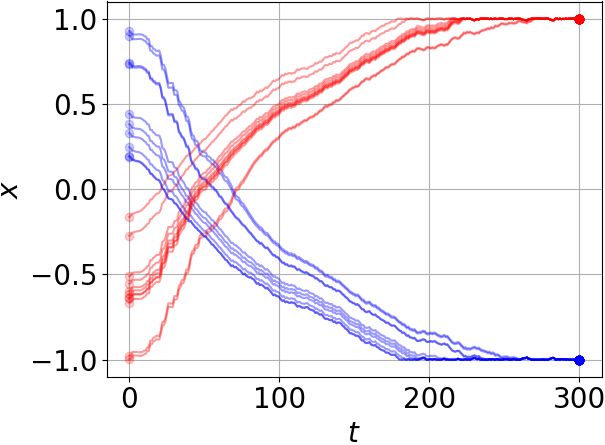
(a) poisoning trajectory

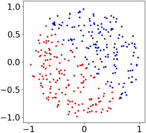
(b) training set

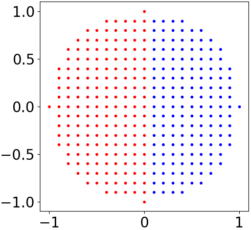
(c) evaluation set

Figure 1: (a) 1D example (b, c) 2D example

We run deep-DPV with $k=n$ for $T=5\times 10^{3}$ iterations. In Figure 2(2(a))-(2(c)), we show the poisoning trajectories for the three attack goals respectively. Each translucent point is an original training point, and the connected solid point is its final position after attack. The curve connecting them shows the trajectory as the attack algorithm gradually poisons the data.

In label-aversion attack the attacker aims to maximize the logistic loss on the evaluation set. It ends up moving positive (negative) items to the left (right), so that the poisoned data deviates from the evaluation set.

In contrast, the label-targeting attack tries to minimize the logistic loss, thus items are moved to produce a poisoned data aligned with the evaluation set. However, the attack does not reproduce exactly the evaluation set. To understand it, we compute the model learnt by vanilla logistic regression on the evaluation set and the poisoned data, which are (2.60,0) and (2.94,0.01). Note that both models can predict the right label on the evaluation set, but the latter has larger norm, which leads to smaller attack cost, thus our result is a better attack.

In parameter-targeting attack, we compute the model learnt by vanilla logistic regression on the clean data and the poisoned data, which are (1.86,1.85) and $(2.21,0.04)$. Note that the attack pushes the model closer to the target model (2.6,0). Again, the attack does not reproduce exactly the evaluation set, which is because the goal is to minimize the attack cost $J=\mathbf{E}_{b}\left[C(\tilde{\theta})\right]$ rather than $C(\tilde{\theta})$. To see that, we evaluate the attack cost $J$ (as explained below) on the evaluation set and the poisoned data, and the values are 2.12 and 1.08 respectively, thus our result is a better attack.

To quantify the attack performance, we evaluate the attack cost $J(\tilde{D})$ via Monte-Carlo sampling. We run private learners $T_{e}=10^{3}$ times, each time with a random $b_{s}$ to produce a cost $C_{s}=C(\mathcal{M}(\tilde{D},b_{s}))$. Then we average to obtain an estimate of the cost $J(\tilde{D})\approx\frac{1}{T_{e}}\sum_{s=1}^{T_{e}}C_{s}$. In Figure 2(2(d))-(2(f)), we show the attack cost $J(\tilde{D})$ and its 95% confidence interval (green, $\pm 2*$stderr) up to $t=10^{3}$ iterations. $J(\tilde{D})$ decreases in all plots, showing that our attack is effective for all attack goals.

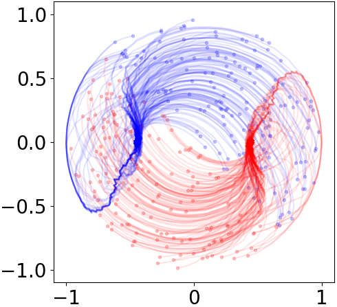
(a) label-aversion

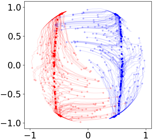
(b) label-targeting

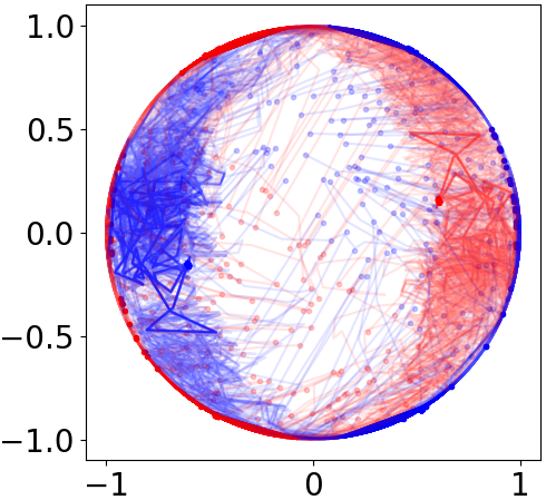
(c) parameter-targeting

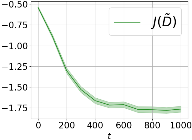
(d) label-aversion

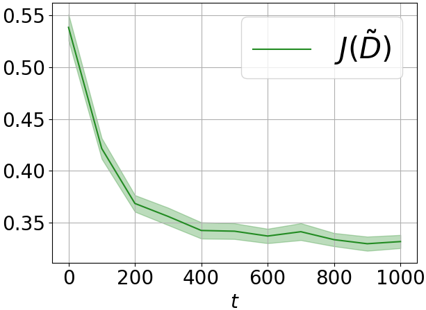
(e) label-targeting

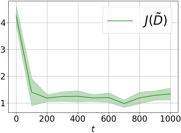
(f) parameter-targeting

Figure 2: poisoning trajectories in 2D.

5.3 Attacks Become More Effective as $k$ Increases

The theoretical protection provided by differential privacy weakens as the adversary is allowed to poison more training items. In this section, we show that our attacks indeed become more effective as the number of poisoned items $k$ increases. The data set is the same as in section 5.2. We run our four attack algorithms with $k$ from 20 to 100 in steps of 20. For each $k$, we first select $k$ items by using shallow or deep selection, and then poison the selected items by running (stochastic) gradient descent for $T=5\times 10^{3}$ iterations. After attack, we estimate the attack cost $J(\tilde{D})$ on $T_{e}=2\times 10^{3}$ samples. Figure 3(3(a))-(3(c)) show that the attack cost $J(\tilde{D})$ decreases as $k$ grows, indicating better attack performance. We also show the poisoning trajectory produced by deep-DPV with $k=10$ in Figure 3(3(d))-(3(f)). The corresponding attack costs $J(\tilde{D})$ are $-0.60,0.49$ and $3.43$ respectively. Compared to that of $k=n$, $-1.79$, $0.32$ and $1.20$, we see that poisoning only 10 items is not enough to reduce the attack cost $J(\tilde{D})$ significantly, although the attacker is making effective modification.

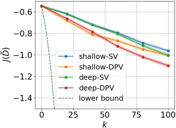
(a) label-aversion

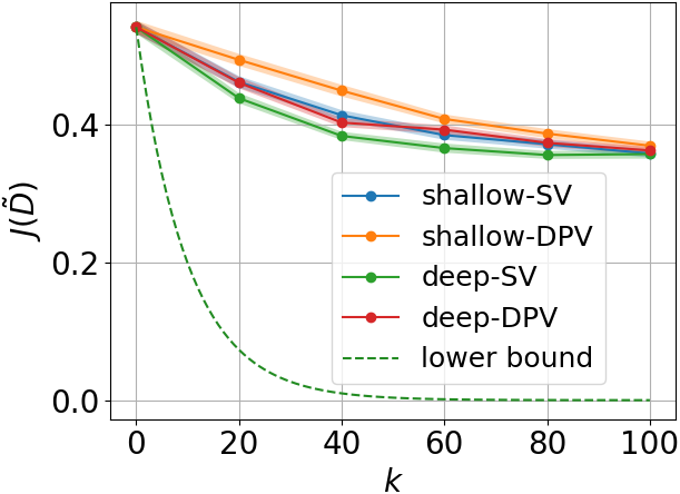
(b) label-targeting

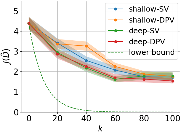
(c) parameter-targeting

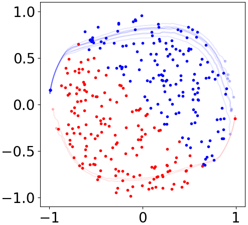
(d) label-aversion

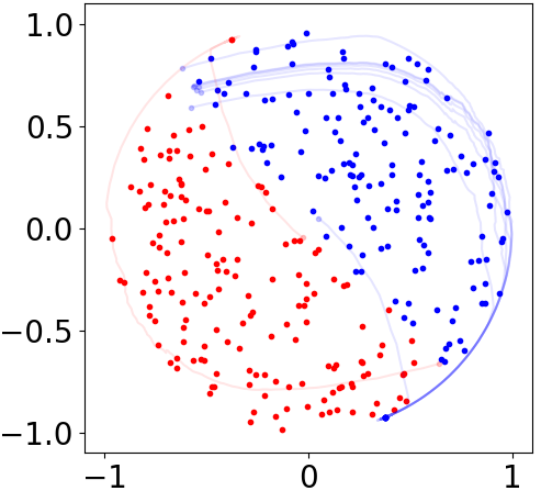
(e) label-targeting

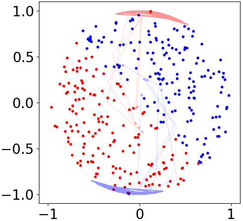
(f) parameter-targeting

Figure 3: (a-c) the attack cost $J(\tilde{D})$ decreases as $k$ grows. (d-f) the sparse attack trajectories for $k=10$

5.4 Attacks Effective on Both Privacy Mechanisms

We now show experiments on real data to illustrate that our attacks are effective on both objective and output perturbation mechanisms. We focus on label-targeting attack in this section.

The first real data set is vertebral column from the UCI Machine Learning Repository [5]. This data set contains 6 features of 310 orthopaedic patients, and the task is to predict if the vertebra of any patient is abnormal (positive class) or not (negative class). We normalize the features so that the norm of any item is at most 1. Since this is a classification task, we use private logistic regression with $\epsilon=0.1$ and $\lambda=10$ as the victim. To generate the evaluation set, we randomly pick one positive item and find its $10$ nearest neighbours within the positive class, and set $y_{i}^{*}=-1$ for all 10. Intuitively, this attack targets a small cluster of abnormal patients and the goal is to mislead the learner to classify these patients as normal. The other experimental parameters remain the same as in section 5.3. Note that in order to push the prediction on $x_{i}^{*}$ toward $y_{i}^{*}$, the attacker requires $y_{i}^{*}{x_{i}^{*}}^{\top}\tilde{\theta}>0$, which indicates $C(\tilde{\theta})=\log(1+\exp(-y_{i}^{*}{x_{i}^{*}}^{\top}\tilde{\theta}))<\log 2\approx 0.69$, so should $J(\tilde{D})$. As shown in Figure 4, the attacker indeed reduces the attack cost $J(\tilde{D})$ below 0.69 for both privacy mechanisms, thus our attack is successful.

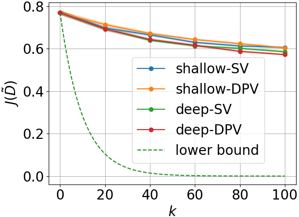
(a) objective perturbation

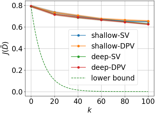
(b) output perturbation

Figure 4: attack on objective and output-perturbed logistic regression.

The second data set is red wine quality from UCI. The data set contains 11 features of 1598 wine samples, and the task is predict the wine quality, a number between 0 and 10. We normalize the features so that the norm of any item is at most 1. Labels are also normalized to ensure the value is in $[-1,1]$. The victim is private ridge regression with $\epsilon=1$, $\lambda=10$, and bound on model space $\rho=2$. To generate the evaluation set, we pick one item $x_{i}^{*}$ with the smallest quality value, and then set the target label to be $y_{i}^{*}=1$. The cost function is defined as $C(\theta)=\frac{1}{2}({x_{i}^{*}}^{\top}\theta-y_{i}^{*})^{2}$. The other parameters of attack remain the same as in section 5.3. This attack aims to force the learner to predict a low-quality wine as having a high quality. Figure 5 shows the results on objective perturbation and output perturbation respectively. Note that the attack cost can be effectively reduced even if the attacker only poisons $100/1598\approx 6.3\%$ of the whole data set.

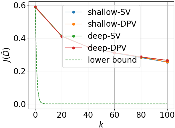
(a) objective perturbation

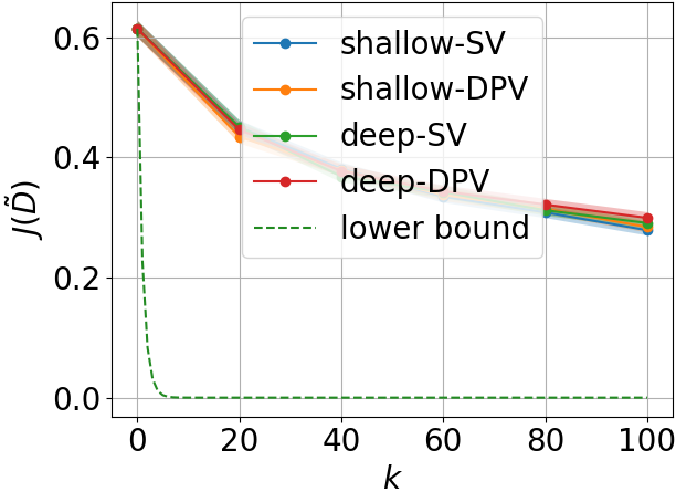
(b) output perturbation

Figure 5: attack on objective and output-perturbed ridge regression.

Given experimental results above, we make another two observations here. First, deep-DPV is in general the most effective method among four attack algorithms, see e.g. Figure 3(3(a)), (3(c)). Second, although deep-DPV is effective, there remains a gap between the attack performance and the theoretical lower bound, as is shown in all previous plots. One potential reason is that the lower bound is derived purely based on the differential privacy property, thus does not take into account the learning procedure of the victim. Analysis oriented toward specific victim learners may result in a tighter lower bound. Another potential reason is that our attack might not be effective enough. How to close the gap is left as future work.

5.5 Attack Is Easier with Weaker Privacy

Finally, we show that the attack is more effective as the privacy guarantee becomes weaker, i.e., as we increase $\epsilon$. To illustrate, we run experiments on the data set in section 5.2, where we fix $k=100$ and vary $\epsilon$ from $0.1$ to $0.5$. In Figure 6, we show the attack cost $J(\tilde{D})$ against $\epsilon$. Note that the attack cost $J(\tilde{D})$ approaches the lower bound as $\epsilon$ grows. This means weaker privacy guarantee (smaller $\epsilon$) leads to easier attacks.

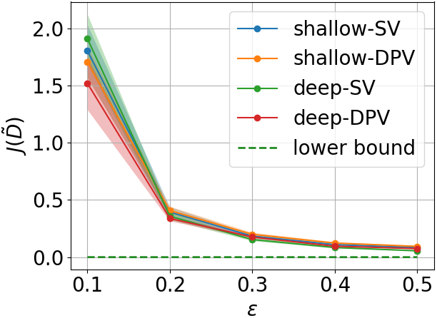
Figure 6: Attacker can reduce cost $J(\tilde{D})$ more as $\epsilon$ grows.

6 Conclusion and Future Work

We showed that differentially private learners are provably resistant to data poisoning attacks, with the protection degrading exponentially as the attacker poisons more items. Then, we proposed attacks that can effectively poison differentially-private learners, and demonstrated the attack performance on a variety of privacy mechanisms and learners with both synthetic and real data. While the attacks are effective, there remains a gap between the theoretical lower bound and the empirical performance of our attacks. This could be because the lower bound is loose, or our attack is not effective enough; closing the gap remains future work. Taken together, our study is a first step towards understanding the strengths and weaknesses of differential privacy as a defensive measure against data poisoning.

Acknowledgements

We thank Steve Wright for helpful discussions. This work is supported in part by NSF 1545481, 1561512, 1623605, 1704117, 1836978, the MADLab AF Center of Excellence FA9550-18-1-0166, a Facebook TAV grant, and the University of Wisconsin.

Appendix: Regularity Condition for Differentiation-Integration Exchange

The following theorem characterizes a sufficient condition when the order of differentiation and integration can be exchanged (restated from Theorem 2.4.3 in [3]), which is called the regularity condition.

Theorem 8.

Suppose $h(z,b)$ is a differentiable function of $z$. If for each $z$, and there exist a function $g(z,b)$ and a constant $d>0$ that satisfy

1. $\|\frac{\partial}{\partial z}h(z,b)\mid_{z=z^{\prime}}\|\leq g(z,b)$, for all $b$ and all $z^{\prime}$ such that $\|z^{\prime}-z\|\leq d$.

2. $\int g(z,b)db<\infty$.

Then for any $z$, we have

$$\frac{d}{dz}\int h(z,b)db=\int\frac{\partial}{\partial z}h(z,b)db.$$ (56)

Note that in condition $i)$, the constant $d$ could depend on $z$ implicitly. Proposition 7 is then a straight-forward corollary of the above theorem by taking function $h$ as $h(\tilde{z}_{i},b)=C(\mathcal{M}(\tilde{D},b))\nu(b)$. The $\nu(b)$ is usually chosen as the Laplace distribution $\nu(b)=\psi e^{-\|b\|}$ for some constant $\psi$, thus from now on we consider $h(\tilde{z}_{i},b)=C(\mathcal{M}(\tilde{D},b))\psi e^{-\|b\|}$. We also require that the poisoned features and labels satisfy $\|\tilde{x}_{i}\|\leq 1$ and $|\tilde{y}_{i}|\leq 1$, to conform with the standard assumption that data must be bounded in differentially private machine learning. Next we use parameter-targeting attack as an example to illustrate that the regularity condition always holds in our attack problem.

1. Attacking objective-perturbed logistic regression.

   In our case, the attacker only modifies the feature, thus we denote $h(\tilde{x}_{i},b)=C(\mathcal{M}(\tilde{D},b))\psi e^{-\|b\|}$. By (37),

   $$\frac{\partial C(\tilde{\theta})}{\partial\tilde{x}_{i}}=\left(\frac{y_{i}}{1+s_{i}}I-\frac{s_{i}\tilde{\theta}\tilde{x}_{i}^{\top}}{(1+s_{i})^{2}}\right)\left(\lambda I+\sum_{j=1}^{n}\frac{s_{j}\tilde{x}_{j}\tilde{x}_{j}^{\top}}{(1+s_{j})^{2}}\right)^{-1}(\tilde{\theta}-\theta^{\prime}),$$ (57)

   where $s_{j}=\exp(y_{j}\tilde{\theta}^{\top}\tilde{x}_{j})$ and $\tilde{\theta}=\mathcal{M}(\tilde{D},b)$. We let $d=1$ in condition $i)$. Note that $\|\tilde{x}_{i}\|\leq 1$, thus for any $\tilde{x}_{i}^{\prime}$ such that $\|\tilde{x}_{i}^{\prime}-\tilde{x}_{i}\|\leq d$, by triangle inequality we have $\|\tilde{x}_{i}^{\prime}\|\leq\|\tilde{x}_{i}\|+d=2$. Let $s_{i}^{\prime}=\exp(y_{i}\tilde{\theta}^{\top}\tilde{x}_{i}^{\prime})$. By (57), we have

   $$\|\frac{\partial C(\tilde{\theta})}{\partial\tilde{x}_{i}}\mid_{\tilde{x}_{i}=\tilde{x}_{i}^{\prime}}\| \leq\|\frac{y_{i}}{1+s_{i}^{\prime}}I-\frac{s_{i}^{\prime}\tilde{\theta}\tilde{x}_{i}^{\prime^{\top}}}{(1+s_{i}^{\prime})^{2}}\|\cdot\|\left(\lambda I+\sum_{\begin{subarray}{c}1\leq j\leq n\\ j\neq i\end{subarray}}\frac{s_{j}\tilde{x}_{j}\tilde{x}_{j}^{\top}}{(1+s_{j})^{2}}+\frac{s_{i}^{\prime}\tilde{x}_{i}^{\prime}\tilde{x}_{i}^{\prime^{\top}}}{(1+s_{i}^{\prime})^{2}}\right)^{-1}\|\cdot\|\tilde{\theta}-\theta^{\prime}\|$$ (58)

   $$\leq\left(\|\frac{y_{i}}{1+s_{i}^{\prime}}I\|+\|\frac{s_{i}^{\prime}\tilde{\theta}\tilde{x}_{i}^{\prime^{\top}}}{(1+s_{i}^{\prime})^{2}}\|\right)\frac{1}{\lambda}(\|\tilde{\theta}\|+\|\theta^{\prime}\|)$$

   $$=\frac{1}{\lambda}\left(\frac{1}{1+s_{i}^{\prime}}+\frac{s_{i}^{\prime}}{(1+s_{i}^{\prime})^{2}}\|\tilde{\theta}\|\|\tilde{x}_{i}^{\prime}\|\right)(\|\tilde{\theta}\|+\|\theta^{\prime}\|)$$

   $$\leq\frac{1}{\lambda}(1+\frac{1}{2}\|\tilde{\theta}\|)(\|\tilde{\theta}\|+\|\theta^{\prime}\|)\quad(\text{since }1+s_{i}^{\prime}\geq 2\sqrt{s_{i}^{\prime}}\text{ and }\|\tilde{x}_{i}^{\prime}\|\leq 2).$$

   Now we upper bound $\|\tilde{\theta}\|$. By (34),

   $$\|\tilde{\theta}\| =\frac{1}{\lambda}\|\sum_{\begin{subarray}{c}1\leq j\leq n\\ j\neq i\end{subarray}}\frac{y_{j}\tilde{x}_{j}}{1+s_{j}}+\frac{y_{i}\tilde{x}_{i}^{\prime}}{1+s_{i}^{\prime}}-b\|\leq\frac{1}{\lambda}(\sum_{\begin{subarray}{c}1\leq j\leq n\\ j\neq i\end{subarray}}\|\frac{y_{j}\tilde{x}_{j}}{1+s_{j}}\|+\|\frac{y_{i}\tilde{x}_{i}^{\prime}}{1+s_{i}^{\prime}}\|+\|b\|)$$ (59)

   $$\leq\frac{1}{\lambda}(n-1+2+\|b\|)=\frac{1}{\lambda}(n+1+\|b\|).$$

   Plugging (59) back to (58), for all $\tilde{x}_{i}^{\prime}$ such that $\|\tilde{x}_{i}^{\prime}-\tilde{x}_{i}\|\leq 1$, we have

   $$\|\frac{\partial C(\tilde{\theta})}{\partial\tilde{x}_{i}}\mid_{\tilde{x}_{i}=\tilde{x}_{i}^{\prime}}\|\leq\frac{1}{\lambda}(1+\frac{n+1+\|b\|}{2\lambda})(\frac{n+1+\|b\|}{\lambda}+\|\theta^{\prime}\|)\leq C_{1}\|b\|^{2},$$ (60)

   for some constant $C_{1}>0$. Therefore

   $$\|\frac{\partial h(\tilde{x}_{i},b)}{\partial\tilde{x}_{i}}\mid_{\tilde{x}_{i}=\tilde{x}_{i}^{\prime}}\|=\|\frac{\partial C(\tilde{\theta})}{\partial\tilde{x}_{i}}\mid_{\tilde{x}_{i}=\tilde{x}_{i}^{\prime}}\|\psi e^{-\|b\|}\leq C_{1}\psi\|b\|^{2}e^{-\|b\|}.$$ (61)

   One can define $g(\tilde{x}_{i},b)=C_{1}\psi\|b\|^{2}e^{-\|b\|}$, which is in fact a function of only $b$, to satisfy condition $i)$ in Theorem 8. Moreover, one can show that $\int g(\tilde{x}_{i},b)db<\infty$, thus condition $ii)$ is also satisfied. Therefore we can exchange the order of differentiation and integration.

2. Attacking objective-perturbed ridge regression.

   We separately show that $h(\tilde{x}_{i},b)$ and $h(\tilde{y}_{i},b)$ satisfy the conditions in Theorem 8.

   First we consider $h(\tilde{x}_{i},b)$. By (44),

   $$\frac{\partial C(\tilde{\theta})}{\partial\tilde{x}_{i}}=\left(\tilde{\theta}\tilde{x}_{i}^{\top}+(\tilde{x}_{i}^{\top}\tilde{\theta}-\tilde{y}_{i})I\right)\left(\tilde{X}^{\top}\tilde{X}+(\lambda+\mu)I\right)^{-1}(\theta^{\prime}-\tilde{\theta}).$$ (62)

   We let $d=1$ in condition $i)$. Note that $\|\tilde{x}_{i}\|\leq 1$, thus $\|\tilde{x}_{i}^{\prime}\|\leq\|\tilde{x}_{i}\|+1\leq 2$. Since $|\tilde{y}_{i}|\leq 1$, $\|\tilde{\theta}\|\leq\rho$, and $\mu\geq 0$, one can easily show that

   $$\|\frac{\partial C(\tilde{\theta})}{\partial\tilde{x}_{i}}\mid_{\tilde{x}_{i}=\tilde{x}_{i}^{\prime}}\|\leq\frac{1}{\lambda}(4\rho+1)(\rho+\|\theta^{\prime}\|).$$ (63)

   Define $g(\tilde{x}_{i},b)=\frac{1}{\lambda}(4\rho+1)(\rho+\|\theta^{\prime}\|)\psi e^{-\|b\|}$. Note that $\int g(\tilde{x}_{i},b)db=\frac{1}{\lambda}(4\rho+1)(\rho+\|\theta^{\prime}\|)<\infty$, thus both condition $i)$ and $ii)$ are satisfied and we can exchange the order of differentiation and integration.

   Next we consider $h(\tilde{y}_{i},b)$. According to (47),

   $$\frac{\partial C(\tilde{\theta})}{\partial\tilde{y}_{i}}=\tilde{x}_{i}^{\top}\left(\tilde{X}^{\top}\tilde{X}+(\lambda+\mu)I\right)^{-1}(\tilde{\theta}-\theta^{\prime}).$$ (64)

   Since $\|\tilde{x}_{i}\|\leq 1$, $\|\tilde{\theta}\|\leq\rho$ and $\mu\geq 0$, one can easily show that for all $\tilde{y}_{i}^{\prime}$,

   $$\|\frac{\partial C(\tilde{\theta})}{\partial\tilde{y}_{i}}\mid_{\tilde{y}_{i}=\tilde{y}_{i}^{\prime}}\|\leq\frac{1}{\lambda}(\rho+\|\theta^{\prime}\|).$$ (65)

   Define $g(\tilde{y}_{i},b)=\frac{1}{\lambda}(\rho+\|\theta^{\prime}\|)\psi e^{-\|b\|}$. Note that $\int g(\tilde{y}_{i},b)db=\frac{1}{\lambda}(\rho+\|\theta^{\prime}\|)<\infty$, thus both condition $i)$ and $ii)$ are satisfied and we can exchange the order of differentiation and integration.

3. Attacking output-perturbed logistic/ridge regression.

   The proof for output-perturbed logistic regression and ridge regression are similar to the objective-perturbed learners, thus we omit them here.

For other attack goals such as label-aversion attack and label-targeting attack, the regularity condition also holds and the proof is similar.

References

- Alfeld et al. [2016] Scott Alfeld, Xiaojin Zhu, and Paul Barford. Data poisoning attacks against autoregressive models. In Thirtieth AAAI Conference on Artificial Intelligence, 2016.
- Biggio et al. [2012] Battista Biggio, Blaine Nelson, and Pavel Laskov. Poisoning attacks against support vector machines. arXiv preprint arXiv:1206.6389, 2012.
- Casella and Berger [2002] George Casella and Roger L Berger. Statistical inference, volume 2. Duxbury Pacific Grove, CA, 2002.
- Chaudhuri et al. [2011] Kamalika Chaudhuri, Claire Monteleoni, and Anand D Sarwate. Differentially private empirical risk minimization. Journal of Machine Learning Research, 12(Mar):1069–1109, 2011.
- Dua and Karra Taniskidou [2017] Dheeru Dua and Efi Karra Taniskidou. UCI machine learning repository, 2017. URL http://archive.ics.uci.edu/ml.
- Dwork [2011] Cynthia Dwork. Differential privacy. Encyclopedia of Cryptography and Security, pages 338–340, 2011.
- Dwork et al. [2006] Cynthia Dwork, Frank McSherry, Kobbi Nissim, and Adam Smith. Calibrating noise to sensitivity in private data analysis. In Theory of cryptography conference, pages 265–284. Springer, 2006.
- Fredrikson et al. [2015] Matt Fredrikson, Somesh Jha, and Thomas Ristenpart. Model inversion attacks that exploit confidence information and basic countermeasures. In Proceedings of the 22nd ACM SIGSAC Conference on Computer and Communications Security, pages 1322–1333. ACM, 2015.
- Jun et al. [2018] Kwang-Sung Jun, Lihong Li, Yuzhe Ma, and Jerry Zhu. Adversarial attacks on stochastic bandits. In Advances in Neural Information Processing Systems, pages 3644–3653, 2018.
- Kifer et al. [2012] Daniel Kifer, Adam Smith, and Abhradeep Thakurta. Private convex empirical risk minimization and high-dimensional regression. In Conference on Learning Theory, pages 25–1, 2012.
- Koh et al. [2018] Pang Wei Koh, Jacob Steinhardt, and Percy Liang. Stronger data poisoning attacks break data sanitization defenses. arXiv preprint arXiv:1811.00741, 2018.
- Lecuyer et al. [2018] Mathias Lecuyer, Vaggelis Atlidakis, Roxana Geambasu, Daniel Hsu, and Suman Jana. Certified robustness to adversarial examples with differential privacy. In Certified Robustness to Adversarial Examples with Differential Privacy. IEEE, 2018.
- Li et al. [2016] Bo Li, Yining Wang, Aarti Singh, and Yevgeniy Vorobeychik. Data poisoning attacks on factorization-based collaborative filtering. In Advances in Neural Information Processing Systems (NIPS), pages 1885–1893, 2016.
- Mei and Zhu [2015] Shike Mei and Xiaojin Zhu. Using machine teaching to identify optimal training-set attacks on machine learners. In The 29th AAAI Conference on Artificial Intelligence, 2015.
- Muñoz-González et al. [2017] Luis Muñoz-González, Battista Biggio, Ambra Demontis, Andrea Paudice, Vasin Wongrassamee, Emil C Lupu, and Fabio Roli. Towards poisoning of deep learning algorithms with back-gradient optimization. In Proceedings of the 10th ACM Workshop on Artificial Intelligence and Security, pages 27–38. ACM, 2017.
- Nozari et al. [2016] Erfan Nozari, Pavankumar Tallapragada, and Jorge Cortés. Differentially private distributed convex optimization via objective perturbation. In 2016 American Control Conference (ACC), pages 2061–2066. IEEE, 2016.
- Raghunathan et al. [2018] Aditi Raghunathan, Jacob Steinhardt, and Percy Liang. Certified defenses against adversarial examples. arXiv preprint arXiv:1801.09344, 2018.
- Steinhardt et al. [2017] Jacob Steinhardt, Pang Wei W Koh, and Percy S Liang. Certified defenses for data poisoning attacks. In Advances in Neural Information Processing Systems (NIPS), pages 3517–3529, 2017.
- Szegedy et al. [2013] Christian Szegedy, Wojciech Zaremba, Ilya Sutskever, Joan Bruna, Dumitru Erhan, Ian Goodfellow, and Rob Fergus. Intriguing properties of neural networks. arXiv preprint arXiv:1312.6199, 2013.
- Tramèr et al. [2016] Florian Tramèr, Fan Zhang, Ari Juels, Michael K Reiter, and Thomas Ristenpart. Stealing machine learning models via prediction apis. In 25th USENIX Security Symposium, pages 601–618, 2016.
- Xiao et al. [2015] Huang Xiao, Battista Biggio, Gavin Brown, Giorgio Fumera, Claudia Eckert, and Fabio Roli. Is feature selection secure against training data poisoning? In International Conference on Machine Learning, pages 1689–1698, 2015.
- Zhang and Zhu [2019] Xuezhou Zhang and Xiaojin Zhu. Online data poisoning attack. arXiv preprint arXiv:1903.01666, 2019.
- Zhao et al. [2017] Mengchen Zhao, Bo An, Wei Gao, and Teng Zhang. Efficient label contamination attacks against black-box learning models. In IJCAI, pages 3945–3951, 2017.