Asymptotic confidence sets for the jump curve
in bivariate regression problems

Abstract

We construct uniform and point-wise asymptotic confidence sets for the single edge in an otherwise smooth image function which are based on rotated differences of two one-sided kernel estimators. Using methods from M-estimation, we show consistency of the estimators of location, slope and height of the edge function and develop a uniform linearization of the contrast process. The uniform confidence bands then rely on a Gaussian approximation of the score process together with anti-concentration results for suprema of Gaussian processes, while point-wise bands are based on asymptotic normality. The finite-sample performance of the point-wise proposed methods is investigated in a simulation study. An illustration to real-world image processing is also given.

1 Introduction

Statistical methodology, in particular nonparametric regression, plays an important role nowadays in image reconstruction and denoising. In two-dimensional image functions, interest often focuses on the location of edges, i.e., discontinuity curves of the intensity function of the image. Edge estimation has been studied in the statistics literature from a minimax point-of-view in the monograph by Korostelev and Tsybakov [11]. Qiu [24] gives an overview of more practical reconstruction methods, which are partially motivated from the literature on computer vision.

Apart from mere estimation, statistical modeling allows for the construction of confidence regions, in which the object of interest is located with high probability. In this paper, we construct asymptotic confidence sets for the single edge in an otherwise smooth image function based on the rotational difference kernel method by Qiu [22] and Müller and Song [15], which is related to the Sobel edge detector from the image processing literature [23].

Confidence sets are by now well-developed for various problems in nonparametric statistics, e.g., for nonparametric density estimation [2, 9, 4], smooth regression functions [6, 18], and deconvolution and errors-in-variables problems [3, 20, 5]. Mammen and Polonik [13] and Qiao and Polonik [21] focus on more geometrical features, and construct confidence regions for density level sets and the density ridge, respectively.

When studying nonparametric regression problems with discontinuities, the focus may either be on the detection of potential jumps, or, assuming the existence of jumps, on estimation and the construction of confidence sets. In the univariate setting with a regression curve having a single jump, the latter problem was studied under various design assumptions by Müller [14], Loader [12], Gijbels et al. [8] and Seijo and Sen [26], among others. The problem of jump detection was additionally addressed, e.g., in [16, 30, 28, 19].

In bivariate problems, Korostelev and Tsybakov [11], Müller and Song [15], Qiu and Yandell [25], Qiu [23], and Garlipp and Müller [7] focus on the estimation of a given discontinuity curve, while Wang [29], Qiu and Yandell [25], Kang and Qiu [10] and Qiu [23] also investigate edge detection. In the latter three papers, the set of jump-location curves is estimated as a point-set, where a certain criterion function exceeds a threshold value.

However, currently there seem to be no methods available to construct a confidence set for the edge in the bivariate case. Our approach to this problem uses the criterion function of the rotational difference kernel method [22, 15], for which we obtain necessary additional kernel conditions for asymptotic normality. The uniform confidence bands then rely on a Gaussian approximation of the score process together with anti-concentration results for suprema of Gaussian processes from Chernozhukov et al. [4], while point-wise bands are based on asymptotic normality. A technical difficulty in the problem are the distinct rates of the estimators of location and slope. As a byproduct of our analysis, we obtain uniform rates of convergence for the estimators of the jump-location-curve, the slope-curve as well as the height-curve which are optimal up to a logarithmic factor.

The paper is structured as follows. In Section 2 we introduce the model as well as the estimators for location and slope of the edge. The main theoretical results can be found in Section 3. Outlines of the proofs for these results are provided in Section 6. Section 4 contains a simulation study and an illustrative application of the proposed method to a real-world image, while Section 5 concludes. Detailed proofs are provided in the Online Supplement [1].

We shall use the following notation. If a sequence of random variables $X_{1},X_{2},\ldots$ converges in probability to a random variable $X$, we write $X_{n}\stackrel{{\scriptstyle\text{P}}}{{\to}}X$ or $X_{n}=X+o_{P}(1)$. If the convergence is in distribution, we write $X_{n}\rightsquigarrow X$. Let $\lambda_{d}$ denote the $d$-dimensional Lebesgue measure. For $d\in\mathbb{N},$ $\mu\in\mathbb{R}^{d},\Sigma\in\mathbb{R}^{d\times d}$ symmetric and positive definite, let $\mathcal{N}_{d}(\mu,\Sigma)$ be the normal distribution with expectation $\mu$ and covariance matrix $\Sigma.$ For a vector $\mathbf{a}\in\mathbb{R}^{d}$, we denote by ${\rm diag}(\mathbf{a})$ the $d\times d$ diagonal matrix with diagonal entries $\mathbf{a}$. Given $\alpha\in(0,1)$, we denote by $q_{\alpha}(X)$ the $\alpha$-quantile of a random variable $X$ resp.  by $q_{\alpha}(Q)$ the $\alpha$-quantile of a distribution $Q$. Let $\langle\,\cdot,\cdot\,\rangle$ denote the Euclidean scalar product on $\mathbb{R}^{d}$.

2 Model and notation

We consider a boundary fragment of a noisy gray scale image, in which real-valued random variables $Y_{i_{1},i_{2}}$ are observed according to the model defined, for all $(i_{1},i_{2})\in\{1,\ldots,n\}\times\{1,\ldots,n\}$, by

$$Y_{i_{1},i_{2}}=m_{\phi}(\mathbf{x_{i_{1},i_{2}}})+\boldsymbol{{\varepsilon}}_{i_{1},i_{2}},$$ (1)

where $\mathbf{x_{i_{1},i_{2}}}=(x_{i_{1}},x_{i_{2}})^{\top}$ form a deterministic, regular rectangular grid in $[0,1]^{2},$ and $m_{\phi}$ is an unknown square-integrable function on $[0,1]^{2},$ which is sufficiently smooth besides a discontinuity curve $\phi$. Specifically, we assume that $m_{\phi}$ is of the form

$$\begin{split}m_{\phi}(x,y)&=m(x,y)+j_{\tau,\phi}(x,y),\\ j_{\tau,\phi}(x,y)&=j_{\tau}(x,y)=\tau(x)\mathbf{1}_{[0,\phi(x)]}(y),\end{split}$$ (2)

where $m:[0,1]^{2}\to\mathbb{R}$ is the smooth part of the image, $\tau:[0,1]\to\mathbb{R}_{+}$ the jump-height curve and $\phi:[0,1]\to(0,1)$ the jump-location curve.

To estimate $\phi(x)$, define the rotation matrix

$$\boldsymbol{\mathscr{R}}_{\psi}=\left(\begin{array}[]{cc}\cos(\psi)&\sin(-\psi)\\ \sin(\psi)&\cos(\psi)\end{array}\right),$$ (5)

where $\psi\in\mathbb{R}$. Further, for a bandwidth $h>0$ and $\mathbf{z}=(z_{1},z_{2})^{\top}\in\mathbb{R}^{2}$, consider the rotated difference kernel

$$K(\mathbf{z};\psi,h)=K(h^{-1}\boldsymbol{\mathscr{R}}_{-\psi}\mathbf{z})/h^{2},$$

where $K(\mathbf{z})=K(z_{1},z_{2})=K_{1}(z_{1})K_{2}(z_{2})$ is a product kernel of univariate kernel functions $K_{1}$ and $K_{2}$, and $K_{1}$ is even while $K_{2}$ is odd and hence corresponds to the difference of two one-sided kernels.

Define for $\mathbf{z}\in[0,1]^{2}$ and $\psi\in[-\pi/2,\pi/2]$ the contrast process with Priestley–Chao-type weights as

$$\hat{\text{M}}_{n}(\mathbf{z};\psi,h)=n^{-2}\sum\limits_{i_{1},i_{2}=1}^{n}Y_{i_{1},i_{2}}K(\mathbf{z}-\mathbf{x_{i_{1},i_{2}}};\psi,h).$$ (6)

For an $x\in(0,1)$ denote by $\psi(x)=\arctan\{\phi^{\prime}(x)\}$ the slope of the tangent at $\phi(x)$. An estimator for the bivariate parameter $(\phi(x),\psi(x))$ is then given by

$$(\hat{\phi}_{n}(x),\hat{\psi}_{n}(x))\in\underset{y\in[h,1-h],\psi\in[-\pi/2,\pi/2]}{\operatorname{arg}\,\operatorname{max}}\;\hat{\text{M}}_{n}((x,y)^{\top};\psi,h).$$ (7)

Our estimator for the jump-height at $x$ is given by

$$\hat{\tau}_{n}(x)=\hat{\text{M}}_{n}((x,\hat{\phi}_{n}(x))^{\top};\hat{\psi}_{n}(x),h).$$

An illustration of the mechanism in (7) is given in Figure 1. The line within the kernel window indicates that the odd kernel $K_{2}$ corresponds to the difference of two one-sided kernels. In order to maximize the contrast $\hat{\text{M}}_{n}(\mathbf{z};\psi,h)$, that is the difference of two one-sided estimators, for fixed $x\in(0,1)$ the kernel window is rotated so that the red line is tangential to the edge.

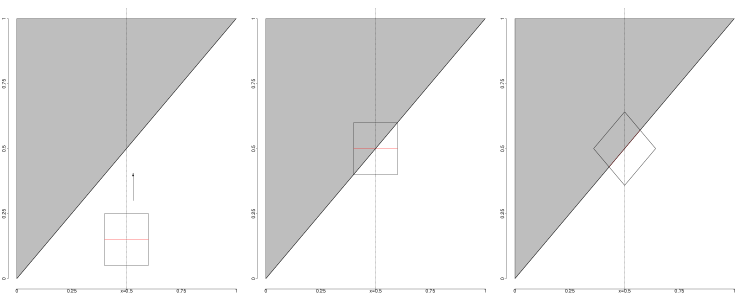
Figure 1: Illustration of rotated difference kernel estimation for a linear jump-location-curve.

Remark 1.

The general idea of this estimator was stated in [22], and in [7] the estimator was made precise by changing the order of scaling and rotating. As initially proposed by [22] one could also use a Gasser–Müller type version of the rotational difference kernel estimator defined by

$$\hat{\text{M}}_{n}(\mathbf{z};\psi,h)=\sum\limits_{i_{1},i_{2}=1}^{n}Y_{i_{1},i_{2}}\int_{\triangle_{i_{1},i_{2}}}K(\mathbf{z}-\mathbf{u};\psi,h)\mathrm{d}\mathbf{u},$$

where $\triangle_{i_{1},i_{2}}=[(i_{1}-1)/n,i_{1}/n)\times[(i_{2}-1)/n,i_{2}/n)$ denotes a design square. However, due to the rectangular fixed design it is easier to analyze the contrast function in (6) instead.

Remark 2 (Several jump curves).

Also of interest for applications is an extension to several jump-location-curves, viz.

$$m_{\phi}(x,y)=m(x,y)+\sum_{k=1}^{J}j_{\tau_{k},\phi_{k}}(x,y),\\$$

and, for all $k\in\{1,\ldots,J\}$,

$$j_{\tau_{k},\phi_{k}}(x,y)=\tau_{k}(x)\mathbf{1}_{[0,\phi_{k}(x)]}(y),$$

where $J\in\mathbb{N}$, $m:[0,1]^{2}\to\mathbb{R}$ is the smooth part of the image, $\tau_{k}:[0,1]\to\mathbb{R}_{+}$ are the jump-height curves and $\phi_{k}:[0,1]\to(0,1)$ are the jump-location-curves. In order to guarantee identification, one has to assume that the images of the jump curves are well separated, i.e., that $B_{\rho}(\phi_{i}[0,1])\cap B_{\rho}(\phi_{j}[0,1])=\emptyset$ for $i,j\in\{1,\ldots,J\}$ with $i\neq j$ and some $\rho>0$, where $B_{\rho}(A)$ denotes the $\rho$-neighborhood of a set $A\subseteq\mathbb{R}$. The theoretical concepts below should be transferable with additional notational effort (see, e.g., Remark 2.6 in [22]) and confidence bands could be constructed based on a Bonferroni-correction. Section 4 illustrates this idea by means of a simulated data example.

Remark 3 (Closed jump curves).

The rotated difference kernel method can also be applied to closed curves as follows. Let $G\subseteq\{x\in\mathbb{R}^{2}:\ \|x\|_{2}\leq 1\}$ be a nonempty, compact, convex set with $0\in\text{int}(G)$ and assume that the image function is given by

$$m_{G}\{x_{\gamma}(t)\}=m\{x_{\gamma}(t)\}+\tau(\gamma)\mathbf{1}_{G}\{x_{\gamma}(t)\},$$

where $m:[-1,1]^{2}\to\mathbb{R}$ is the smooth part, $\tau:[0,2\pi)\to\mathbb{R}_{+}$ is the jump height and the location $x_{\gamma}$ is given by $x_{\gamma}:[0,1]\to[-1,1]^{2}:t\mapsto t(\cos(\gamma),\sin(\gamma))^{\top}$ with $\gamma\in[0,2\pi)$. Now for $\gamma\in[0,2\pi),\psi\in[-\pi/2,\pi/2]$, consider the estimator

$$(\hat{\phi}_{n}(\gamma),\hat{\psi}_{n}(\gamma))\in\underset{t\in[h,1-h],\psi\in[-\pi/2,\pi/2]}{\operatorname{arg}\,\operatorname{max}}\;\sum\limits_{i_{1},i_{2}=1}^{n}Y_{i_{1},i_{2}}K(x_{\gamma}(t)-\mathbf{x_{i_{1},i_{2}}};\psi,h).$$

While details need to be worked out, our asymptotic analysis below should be transferable to this model.        

3 Asymptotic theory

For our asymptotic analysis, we require the following set of assumptions.

Assumption 1 (Errors).

The errors $\boldsymbol{{\varepsilon}}_{i_{1},i_{2}}$ are square-integrable, centered, independent and identically distributed random variables with common variance $\sigma^{2}.$ Moreover, ${\rm E}|\epsilon_{1,1}|^{5}<\infty.$ ∎

Assumption 2 (Smoothness).

We have that $\phi\in C^{2}[0,1],\tau\in C^{2}[0,1]$ and $m\in C^{2}[0,1]^{2}.$ ∎

Assumption 3 (Bandwidth).

The bandwidth $h=h_{n}$ lies in the range $[{C_{1}\ln(n)^{\eta}}/{n^{1/2}},{C_{2}}/{n^{1/3}}]$ for some finite constants $C_{1},C_{2}>0$ and some fixed $\eta>1.$ ∎

Assumption 4 (Kernel).

The kernel functions $K_{1}$ and $K_{2}$ are three-times continuously differentiable with support in $[-1,1]$ and satisfy the following conditions.

1. $K_{1}$ is symmetric, i.e., $K_{1}(x)=K_{1}(-x)$, and $K_{1}(x)>0$ for $x\in(-1,1)$. Further, $K_{1}$ satisfies, for all $j\in\{0,1,2\}$,

   $$\int_{[-1,1]}K_{1}(x)\mathrm{d}x=1\quad\text{and}\quad K_{1}^{(j)}(-1)=K_{1}^{(j)}(1)=0.$$

2. $K_{2}$ is an odd function, i.e., $K_{2}(x)=-K_{2}(-x)$, in particular $K_{2}(0)=0$, and satisfies, for all $j\in\{0,1,2\}$,

   $$\int_{0}^{1}K_{2}(x)\mathrm{d}x =-\int_{-1}^{0}K_{2}(x)\mathrm{d}x=1,\ K_{2}^{(1)}(0)>0\quad\text{and}\quad K_{2}^{(j)}(-1)=K_{2}^{(j)}(1)=0.$$

∎

Assumption 5 (Kernel moment).

$K_{2}$ satisfies $\int_{0}^{1}xK_{2}(x)\mathrm{d}x=0.$ ∎

Remark 4 (Assumptions).

• Assumption 1 could be relaxed to ${\rm E}|\varepsilon_{1,1}|^{k}<\infty$ for some $k>4/(2-\delta)$ and $\delta\in(2/3,1],$ as can be seen from the Gaussian approximation provided in the Online Supplement; see (LABEL:eq_approx_rio) therein. However, this would introduce a new parameter $\delta,$ which in turn has to be taken into account for the range of admissible bandwidths and thus for sake of convenience we require the slightly stronger assumptions of existing fifth moments which is sufficient for the bandwidth range in Assumption 3.

• Assumptions 2–4 are required for the asymptotic distribution of the jump-location estimate $\hat{\phi}_{n}$ in (7), whereas Assumption 5 is only needed for the faster rates of convergence of the estimates $\hat{\psi}_{n}$ and $\hat{\tau}_{n}.$ Under Assumption 2 the moment properties of $K_{1}$ resp. $K_{2}$ in Assumption 4 (resp. 5) eliminate lower order terms in Taylor expansions, similarly as for higher order kernels in standard kernel smoothing. We also point out that Assumption 3 corresponds to an undersmoothing for the continuous part of the image function. In particular, we require $nh_{n}^{2}\to\infty$ and $nh_{n}^{3}\to\text{const.},$ a standard assumption in bivariate nonparametric estimation for Lipschitz functions. Finally, note that $\ln(n)$ and $\ln(h^{-1})$ are of the same order.

• Our new conditions in Assumption 4 are necessary for asymptotic normality of the estimates based on the rotated difference kernel method.

In the following, we fix some compact subinterval $I\subset(0,1)$. Let us start with uniform consistency of the estimators on $I$.

Theorem 1.

In model (1), under Assumptions 1–4 we have that

$$\sup_{x\in I}\ \big{|}\hat{\phi}_{n}(x)-\phi(x)\big{|}=O_{P}\{{\ln(n)^{1/2}}/{n}\}.$$

If in addition Assumption 5 holds, then

$$\sup_{x\in I}\ \big{|}\hat{\psi}_{n}(x)-\psi(x)\big{|}=O_{P}\{{\ln(n)^{1/2}}/{(nh)}\},\quad \sup_{x\in I}\ \big{|}\hat{\tau}_{n}(x)-\tau(x)\big{|}=O_{P}\{{\ln(n)^{1/2}}/{(nh)}\}.$$

Remark 5 (Rates of convergence and optimality).

Theorem 1 shows that with our kernel assumptions, i.e., Assumption 3, the estimator for the jump location achieves the optimal rate of convergence up to a logarithmic factor, see Theorem 3.3.1 in [11] for the corresponding lower bound. Note that this is faster than the rates in Remark 2.4 in [22], who lacks the kernel conditions in his asymptotic analysis.

Although there seem to be no rigorous results on lower bounds available, it is reasonable to believe that the rates for the jump-slope curve and the jump-height curve are optimal up to a logarithmic term as well, since these correspond to the uniform rate for estimating Lipschitz continuous functions.

Now we turn to asymptotic normality of $\hat{\phi}_{n}(x)$ for fixed $x$. To state a version which does not involve a bias correction, we require the maximizer of the deterministic version of the contrast function

$$\phi_{n}(x)\in\underset{y\in[h,1-h]}{\operatorname{arg}\,\operatorname{max}}\;\max_{\psi\in[-\pi/2,\pi/2]}{\rm E}\{\hat{\text{M}}_{n}((x,y)^{\top};\psi,h)\}.$$

Theorem 2.

In model (1), under Assumptions 1–4 we have, for any $x\in I$, that as $n\to\infty$,

$$n\{\hat{\phi}_{n}(x)-\phi_{n}(x)\}\rightsquigarrow\mathcal{N}[0,\sigma^{2}\ V_{\phi}^{S}(x)/\{V_{\phi}^{H}(x)\}^{2}],$$

where

$$\begin{split}V_{\phi}^{H}(x)&=\tau(x)\cos^{2}\{\psi(x)\}K_{2}^{(1)}(0),\\ V_{\phi}^{S}(x)&=\sin^{2}\{\psi(x)\}\int_{[-1,1]^{2}}\{K_{1}^{(1)}(z_{1})K_{2}(z_{2})\}^{2}\mathrm{d}z_{1}\mathrm{d}z_{2}+\cos^{2}\{\psi(x)\}\int_{[-1,1]^{2}}\{K_{1}(z_{1})K_{2}^{(1)}(z_{2})\}^{2}\,\mathrm{d}z_{1}\mathrm{d}z_{2}.\end{split}$$ (8)

We even obtain joint asymptotic normality and asymptotic independence of $(\hat{\phi}_{n},\hat{\psi}_{n},\hat{\tau}_{n})$; see the proofs section, Theorem 4. In (8), $V_{\phi}^{H}(x)$ arises as a limit of the Hessian matrices, while $V_{\phi}^{S}(x)$ comes from the asymptotic variance of the score.

Remark 6 (Confidence intervals).

In order to construct asymptotic confidence intervals, we choose a consistent estimate $\hat{\sigma}^{2}_{n}$ of the error variance $\sigma^{2}$; see, e.g., Munk et al. [17] and the simulations in Section 4. Given $\alpha\in(0,1)$, we obtain an asymptotic level $1-\alpha$ confidence interval for $\phi_{n}(x)$ by computing

$$\left[\hat{\phi}_{n}(x)-\frac{\hat{\sigma}_{n}\sqrt{V_{\widehat{\phi}}^{S}(x)}q_{1-\alpha/2}}{nV_{\widehat{\phi}}^{H}(x)},\ \hat{\phi}_{n}(x)+\frac{\hat{\sigma}_{n}\sqrt{V_{\widehat{\phi}}^{S}(x)}q_{1-\alpha/2}}{nV_{\widehat{\phi}}^{H}(x)}\right],$$ (9)

where $q_{\beta}=q_{\beta}(\mathcal{N}_{1}(0,1))$ is the $\beta$-quantile of $\mathcal{N}(0,1)$ and where we substitute estimators for the unknown parameters in (8),

$$V_{\widehat{\phi}}^{H}(x) =\hat{\tau}_{n}(x)\cos^{2}\{\hat{\psi}_{n}(x)\}K_{2}^{(1)}(0),$$ (10)

$$\quad V_{\widehat{\phi}}^{S}(x) =\sin\big{(}\hat{\psi}_{n}(x)\big{)}^{2}\int_{[-1,1]^{2}}\{K_{1}^{(1)}(z_{1})K_{2}(z_{2})\}^{2}\mathrm{d}z_{1}\mathrm{d}z_{2}+\ \cos\{\hat{\psi}_{n}(x)\}^{2}\int_{[-1,1]^{2}}\{K_{1}(z_{1})K_{2}^{(1)}(z_{2})\}^{2}\mathrm{d}z_{1}\mathrm{d}z_{2}.$$

Remark 7 (Bias correction).

The proofs show that there exists a bounded sequence $b_{n}$ such that, as $n\to\infty$,

$$n\{\hat{\phi}_{n}(x)-\phi(x)\}-b_{n}\rightsquigarrow\mathcal{N}[0,\sigma^{2}\ V_{\phi}^{S}(x)/\{V_{\phi}^{H}(x)\}^{2}].$$

An explicit bound on $b_{n}$ based on the Lipschitz constants of $K,m,\phi$ and $\psi$ as well as on $||\,\tau\,||_{\infty}$ would be available by an explicit estimation of the second-order term and the Riemann-sum error term, see Lemma 3 and the expansion (26), and hence bias-corrected conservative confidence intervals could be constructed in a similar fashion as in Eubank and Speckman [6]. Indeed, from Korostelev and Tsybakov [11] it is known that the discretization bias for jump-curve estimation in a deterministic design is not negligible theoretically. However, our simulations show that the confidence intervals in (9) can typically be used for the actual parameter, and a bias correction is not necessary, indeed, it makes the intervals quite conservative.

Now let us turn to the construction of uniform confidence sets. For independent standard normal random variables $\xi_{1,1},\ldots,\xi_{n,n},$ independent of $Y_{i_{1},i_{2}},$ consider the process

$$\begin{split}Z^{\xi}_{n,\widehat{\phi}}(x)&=\frac{1}{nh\{V_{\widehat{\phi}}^{S}(x)\}^{1/2}}\\ &\quad\times\sum\limits_{i_{1},i_{2}=1}^{n}\xi_{i_{1},i_{2}}\langle\,(\nabla K)(h^{-1}\boldsymbol{\mathscr{R}}_{-\hat{\psi}_{n}(x)}\{(x,\hat{\phi}_{n}(x))^{\top}-\mathbf{x_{i_{1},i_{2}}}\}),(\sin\hat{\psi}_{n}(x),\cos\hat{\psi}_{n}(x))^{\top}\,\rangle,\end{split}$$ (11)

where $\nabla K(z_{1},z_{2})=(K_{1}^{(1)}(z_{1})K_{2}(z_{2}),K_{1}(z_{1})K_{2}^{(1)}(z_{2}))^{\top}$ and by definition of the rotation matrix in (5),

$$\boldsymbol{\mathscr{R}}_{-\hat{\psi}_{n}(x)}\{(x,\hat{\phi}_{n}(x))^{\top}-\mathbf{x_{i_{1},i_{2}}}\}=\left(\begin{array}[]{c}\cos\{\hat{\psi}_{n}(x)\}(x-x_{i_{1}})+\sin\{\hat{\psi}_{n}(x)\}\{\hat{\phi}_{n}(x)-x_{i_{2}}\}\\ \cos\{\hat{\psi}_{n}(x)\}\{\hat{\phi}_{n}(x)-x_{i_{2}}\}-\sin\{\hat{\psi}_{n}(x)\}(x-x_{i_{1}})\end{array}\right).$$

This process corresponds to the normalized score process evaluated at the estimates $(\hat{\phi}_{n},\hat{\psi}_{n})$ with independent noise-variables $\xi_{i_{1},i_{2}}$. Furthermore, consider the maximum

$$\mathscr{Z}^{\xi}_{n,\widehat{\phi}}=\sup_{x\in I}\big{|}Z^{\xi}_{n,\widehat{\phi}}(x)\big{|}.$$ (12)

The quantiles of this process can be determined by bootstrap simulations. The following result is the basis for constructing uniform confidence sets.

Theorem 3.

Consider model (1) under Assumptions 1–4, and assume that $\hat{\sigma}_{n}$ is an estimator for $\sigma$ which satisfies $\Pr(|{\hat{\sigma}_{n}}/{\sigma}-1|\geq s_{n})=o(1)$ for some sequence $s_{n}=o\{1/\ln(n)\}$. Then for $\alpha\in(0,1)$, one has $q_{1-\alpha}(\mathscr{Z}^{\xi}_{n,\widehat{\phi}})=O_{P}\{(\ln n)^{1/2}\}$ and for any sequence $t_{n}=o(1)$ such that $t_{n}\sqrt{\ln(n)}\to\infty$, we have that

$$\liminf_{n}\ \Pr\left[\sup_{x\in I}\Big{|}{V_{\widehat{\phi}}^{H}(x)\{\hat{\phi}_{n}(x)-\phi(x)\}}/{\sqrt{V_{\widehat{\phi}}^{S}(x)}}\Big{|}\leq{(1+t_{n})\hat{\sigma}_{n}q_{1-\alpha}(\mathscr{Z}^{\xi}_{n,\widehat{\phi}})}/{n}\right]\geq 1-\alpha.$$ (13)

Remark 8 (Asymptotic confidence bands).

Given $\alpha\in(0,1)$ a confidence band for $\phi$ which is asymptotically conservative at level $1-\alpha$ is given by

$$\{[c_{\phi,u}^{-}(x),c_{\phi,u}^{+}(x)]:\ x\in I\},\quad c_{\phi,u}^{\pm}(x)=\hat{\phi}_{n}(x)\pm{(1+t_{n})\hat{\sigma}_{n}\sqrt{V_{\widehat{\phi}}^{S}(x)}q_{1-\alpha}(\mathscr{Z}^{\xi}_{n,\widehat{\phi}})}/\{nV_{\widehat{\phi}}^{H}(x)\}.$$ (14)

Note that this is a version of the asymptotic point-wise confidence interval in (9), corrected by the logarithmic factor $q_{1-\alpha}(\mathscr{Z}^{\xi}_{n,\widehat{\phi}})$ for uniform coverage. Further, the uniform confidence bands also directly apply to the actual parameter $\phi$, the price to pay being that they are asymptotically conservative. Similarly as in Theorem 3, one can construct uniform confidence bands for $\psi$ and $\tau$. We sketch this in Section 6.9.

Remark 9 (Choice of $t_{n}$).

The factors $t_{n}$ can be interpreted as a bias correction, and are essential for the validity of (13), even though they do not affect the rate of convergence. We will conduct a sensitivity analysis for the choice of $t_{n}$ in Section 4. $t_{n}$ ensures that the confidence bands are asymptotically valid, i.e., the significance level $1-\alpha$ is kept asymptotically, the assumption on $t_{n}$ in Theorem 3 prevents a straightforward analysis of asymptotically correct coverage of the confidence bands as in Corollary 3.1 of [4].

4 Simulations

In this section we investigate the finite sample properties of the proposed asymptotic confidence sets for the location $\phi(x)$ of the edge as well as of the estimator

$$\{\hat{\sigma}_{n}^{2}\times V_{\widehat{\phi}}^{S}(x)/V_{\widehat{\phi}}^{H}(x)^{2}\}^{1/2}$$ (15)

for the asymptotic standard deviation of $n\hat{\phi}_{n}(x)$ in Theorem 2 using (10). Further, we also investigate the bias in the estimation of the edge when using a deterministic rectangular grid.

4.1 Simulation setup

We choose

$$m(x,y)=\sin(y^{2})\cos\{(x-1/2)^{2}\},\quad\tau(x)=3\sin^{2}(10x)/10+1/2,$$

as background image and jump height, and consider the following two edge functions

$$\phi_{1}(x)=1/4+x/2,\quad\phi_{2}(x)=-\left(x-1/2\right)^{2}+3/5,$$

from which we form the regression functions $m_{\phi_{1}}$, $m_{\phi_{2}}$, according to model (2). Further, we choose $\epsilon\sim t_{10}(0,\tilde{\sigma})$, i.e., a Student $t$ distribution with location parameter zero, scale parameter $\tilde{\sigma}$ and $10$ degrees of freedom. Thus, the noise-level is given by $\sigma=\tilde{\sigma}\sqrt{10/8}$. For illustration purposes, we display observations from the two models in Figure 2 for grid size $n^{2}=128^{2}$. We use the kernels

$$K_{1}(x)=C_{1}\exp\{-(1-x^{2})^{-1}\}\mathbf{1}_{[-1,1]}(x),\quad K_{2}(x)=C_{2}\exp\{-(1-x^{2})^{-1}\}(x^{3}-x)\mathbf{1}_{[-1,1]}(x),$$

where $C_{1}$ and $C_{2}$ are normalizing constants such that $\int K_{1}=1$ and $\int_{0}^{1}K_{2}=1$, which satisfy Assumption 4.

For the asymptotic results the bandwidth $h$ need not be chosen according to unknown smoothness parameters, and hence bandwidth selection is not a serious issue from a theoretical point of view. One could choose the bandwidth according to a selection rule like cross-validation or Lepski’s rule to optimally estimate the background image $m$. Qiu [24] discusses simpler, more heuristic alternatives, one of which is to choose the window so that it contains approximately 100 design points. Although this is certainly not a universal rule which works for any $n$, we achieve reasonably good results with this approach for our grid sizes of $n^{2}\in\{128^{2},196^{2},256^{2}\}$. In repeated simulations we use $500$ repetitions.

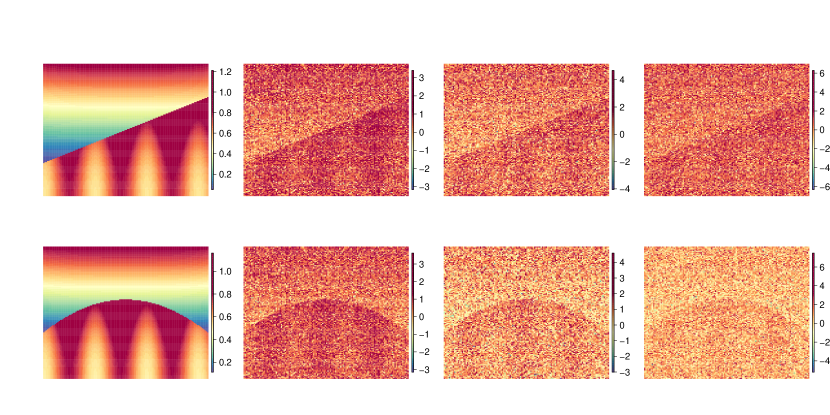
Figure 2: Upper panel: Image function $m_{\phi_{1}}$ with $\tilde{\sigma}=0$, $0.5$, $0.7$, $0.9$ (from left to right) and $n=128$, respectively. Lower panel: Image function $m_{\phi_{2}}$ with $\tilde{\sigma}=0$, $0.5$, $0.7$, $0.9$ (from left to right) and $n=128$, respectively.

4.2 Estimating the asymptotic standard deviation

We start by investigating the numerical performance of the estimator (15) of the asymptotic standard deviation. To this end, we need to specify $\hat{\sigma}_{n}$, for which we choose squares of differences of all neighboring observation pairs properly normalized. The theory in [17] does not immediately apply when estimating on the full image. One possibility is to restrict estimation to a smooth part of the image. We also simulated the estimator $\hat{\sigma}_{n}$ of the standard deviation $\sigma$ separately, the results (not displayed) were also satisfactory.

Figure 3: Asymptotic standard deviation for $n\hat{\phi}_{n}$ (solid lines), and its estimates (dotted-dashed lines). Three leftmost pictures: Standard deviation estimation for the image-function $m_{\phi_{1}}$ for $\tilde{\sigma}=0.5$ and $n=128$, $196$, $256$ (from left to right). Three rightmost pictures: Standard deviation estimation for the image-function $m_{\phi_{2}}$ for $\tilde{\sigma}=0.5$ and $n=128$, $196$, $256$ (from left to right).

Table 1: Root of the MSE of the standard deviation estimate in scenario $\phi_{1}$ for some points $x$ if $\tilde{\sigma}=0.5$ or $\tilde{\sigma}=0.9$. The last row indicates the mean of the RMSE for 64 points in the corresponding setting.

$\phi_{1}$	$\tilde{\sigma}=0.5$				$\tilde{\sigma}=0.9$
$x$	$n=128$	$n=196$	$n=256$	asymp. sd	$n=128$	$n=196$	$n=256$	asymp. sd
0.040	0.104	0.110	0.112	0.888	0.232	0.183	0.201	1.599
0.142	0.101	0.080	0.071	0.611	0.209	0.154	0.119	1.100
0.347	0.144	0.128	0.122	0.913	0.272	0.208	0.200	1.644
0.449	0.107	0.084	0.075	0.617	0.183	0.163	0.136	1.111
0.653	0.186	0.160	0.136	0.935	0.325	0.222	0.244	1.683
0.858	0.160	0.132	0.123	0.725	0.275	0.206	0.204	1.305
	0.148	0.124	0.111		0.264	0.195	0.176

Table 2: Root of the MSE of the standard deviation estimation for some points $x$ if $\tilde{\sigma}=0.5$ resp.  $\tilde{\sigma}=0.9$ and scenario $\phi_{2}$. The last row indicates the mean of the RMSE for 64 points in the corresponding setting.

$\phi_{2}$	$\tilde{\sigma}=0.5$				$\tilde{\sigma}=0.9$
$x$	$n=128$	$n=196$	$n=256$	asymp. sd	$n=128$	$n=196$	$n=256$	asymp. sd
0.040	0.137	0.148	0.153	1.149	0.274	0.244	0.243	2.069
0.142	0.130	0.087	0.087	0.691	0.226	0.170	0.158	1.244
0.347	0.142	0.124	0.132	0.840	0.257	0.196	0.202	1.511
0.449	0.101	0.078	0.067	0.540	0.191	0.133	0.123	0.972
0.653	0.193	0.156	0.143	0.859	0.317	0.238	0.182	1.547
0.858	0.107	0.101	0.100	0.820	0.207	0.168	0.171	1.477
	0.143	0.119	0.111		0.263	0.200	0.182

Next we present the results for (15). Figure 3 shows smoothed estimates for specific samples for grid sizes $n^{2}\in\{128^{2},196^{2},256^{2}\}$ for the two edge functions $\phi_{i}$. Further, in Tables 1 and 2 we plot the square roots of the Mean-Squared-Error (RMSE) of the standard deviation estimates for the three sample sizes and two edge curves at various observation points $x$ based on repetitions. For comparison purposes, the actual asymptotic standard deviation is given as well. One observes that the RMSE in most settings decreases as the number of grid points increases. Further, the magnitude of the RMSE as compared to the actual value of the asymptotic standard deviation is quite small for all cases.

4.3 Confidence intervals and confidence bands

We investigate the coverage behavior and average width of (9) as well as of (14) for the true jump-location curves $\phi_{i}$ in both settings $i\in\{1,2\}$. The results are summarized in Tables 4 and 5 for the noise-levels $\tilde{\sigma}=0.5$ and $\tilde{\sigma}=0.9$. The values in the tables of the point-wise confidence intervals correspond to the average of the respective quantity over 64 design points $x$. The quantile $q_{\beta}(\mathscr{Z}^{\xi}_{n,\widehat{\phi}})$ for $\beta\in(0,1)$ was simulated based on a multiplier bootstrap sample of size $40{,}000$. Furthermore, as there is no explicit representation of the $t_{n}$-term we have chosen it as given in Table 3 for the different scenarios. The $t_{n}$ decrease for increasing sample size $n$ and are of the same magnitude for both scenarios, i.e., for $\phi_{1}$ and $\phi_{2}$. By way of comparison, we give the values of $1/\sqrt{\ln(n)}$ for the different sample sizes $n$ as well. Especially, in the high-noise case the magnitude of our choice for $t_{n}$ is much smaller as this benchmark.

Table 3: Choice of $t_{n}$ in (14).

	$\tilde{\sigma}=0.5$			$\tilde{\sigma}=0.9$
	$n=128$	$n=196$	$n=256$	$n=128$	$n=196$	$n=256$
$\phi_{1}$	0.37	0.34	0.335	0.07	0.001	0
$\phi_{2}$	0.4	0.37	0.25	0.14	0.1	0.06
$1/{\sqrt{\ln(n)}}$	0.45	0.44	0.42	0.45	0.44	0.42

Overall, the simulated coverage probabilities for the point-wise confidence intervals are reasonably close to their nominal values in all scenarios, and the intervals become narrower with increasing numbers of grid points. As expected from the theoretical developments, the uniform confidence bands are somewhat conservative particularly in the high noise-level case.

Table 4: Average coverage and width of the point-wise confidence intervals for the jump-location in (9) for $\tilde{\sigma}=0.5$ and $\tilde{\sigma}=0.9$ over 64 design points.

$\tilde{\sigma}=0.5$					$\tilde{\sigma}=0.9$
	95% nominal coverage		99% nominal coverage		95% nominal coverage		99% nominal coverage
	coverage	width	coverage	width	coverage	width	coverage	width
$n=128$
$\phi_{1}$	0.960	0.025	0.991	0.033	0.943	0.043	0.985	0.056
$\phi_{2}$	0.958	0.025	0.991	0.033	0.946	0.042	0.983	0.056
$n=196$
$\phi_{1}$	0.958	0.016	0.992	0.021	0.944	0.028	0.990	0.037
$\phi_{2}$	0.951	0.016	0.988	0.022	0.943	0.028	0.988	0.037
$n=256$
$\phi_{1}$	0.958	0.012	0.992	0.016	0.941	0.021	0.997	0.028
$\phi_{2}$	0.949	0.013	0.988	0.017	0.949	0.021	0.993	0.029

Table 5: Average coverage and width of the uniform confidence bands for the jump-location in (14) for $\tilde{\sigma}=0.5$ and $\tilde{\sigma}=0.9$.

$\tilde{\sigma}=0.5$					$\tilde{\sigma}=0.9$
	95% nominal coverage		99% nominal coverage		95% nominal coverage		99% nominal coverage
	coverage	width	coverage	width	coverage	width	coverage	width
$n=128$
$\phi_{1}$	0.943	0.051	0.986	0.059	0.955	0.062	0.999	0.071
$\phi_{2}$	0.959	0.049	0.984	0.059	0.945	0.065	0.999	0.075
$n=196$
$\phi_{1}$	0.945	0.032	0.988	0.038	0.954	0.039	0.999	0.045
$\phi_{2}$	0.957	0.032	0.986	0.039	0.948	0.042	1.000	0.050
$n=256$
$\phi_{1}$	0.949	0.025	0.987	0.028	0.951	0.030	0.993	0.032
$\phi_{2}$	0.953	0.025	0.994	0.033	0.955	0.032	0.999	0.039

Figure 4 illustrates the estimated curve as well as the confidence intervals and bands for $\phi_{1}$ and $\phi_{2}$ in the low noise-level for increasing numbers of grid points for $\alpha=0.05$, that is, asymptotic $95\%$ coverage probability. Apparently, the variability of the jump-location estimator decreases and the confidence intervals or bands become narrower. Besides, the confidence bands adapt to the shape of the point-wise confidence intervals as the width-terms only differ in the choice of the quantile.

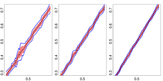
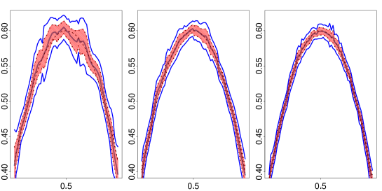
Figure 4: Top panel: 95% Confidence intervals and estimate of the jump-location curve (shaded area and solid line within), uniform confidence bands (solid lines) and true jump-location curve $\phi_{1}$ (dashed lines inside shaded area) for $n=128,$ $196,$ $256$ and $\tilde{\sigma}=0.5$. Lower panel: 95% Confidence intervals and estimate of the jump-location curve (shaded area and solid line within), uniform confidence bands (solid lines) and true jump-location curve $\phi_{2}$ (dashed lines inside shaded area) for $n=128,$ $196,$ $256$ and $\tilde{\sigma}=0.5$.

4.4 Sensitivity analysis of $t_{n}$

In order to get some insight on the role of the sequence $t_{n},$ we display in Figure 5 the empirical quantiles of

$$\sup_{x\in I}\ n\times\Big{|}\frac{V_{\widehat{\phi}}^{H}(x)\{\hat{\phi}_{n}(x)-\phi(x)\}}{\hat{\sigma}_{n}\sqrt{V_{\widehat{\phi}}^{S}(x)}}\Big{|}$$ (16)

together with the simulated quantile curve $\{q_{1-\alpha}(\mathscr{Z}^{\xi}_{n,\widehat{\phi}}):\alpha\in(0,1)\}$ for $\phi_{1}$ (the results for $\phi_{2}$ were similar). The simulated quantile curve is below the empirical quantile curve in particular for the low-noise level, while in the high noise-level the bootstrapped quantile curve is below the empirical quantile curve only for values smaller than a unique intersection point at approximately $0.95,$ and from then on above the empirical quantile curve. Thus, to guarantee an appropriate coverage of the confidence bands the bias correction term $t_{n}$ sequence must be of a higher magnitude in the low-noise level than in the high-noise level. Heuristically this is reasonable as the presence of the bias is much more noticeable in the low-noise case than in the high-noise case. The asymptotic choice $1/\sqrt{\ln(n)}$ would lead to valid but conservative confidence bands.

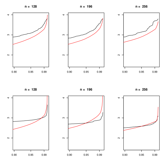
Figure 5: Empirical quantiles of (16) for $\phi_{1}$ (black solid lines) and the corresponding bootstrapped quantiles (red solid line) for sample sizes $n\in\{128,196,256\}.$ Top panel: low-noise case $\tilde{\sigma}=0.5.$ Bottom panel: high-noise case $\tilde{\sigma}=0.9.$

4.5 Comparing bias and standard deviation

Next, we investigate the order of the bias numerically and compare it to the standard deviation. Tables 6 and 7 contain the results for the ratio of the bias and the standard deviation for different design points $x$ in the low noise-level and the high noise-level case. The ratios are quite small, showing that the bias indeed is often of smaller magnitude than the standard deviation.

Table 6: Ratio between computed bias and estimated standard deviation for different points $x$ in scenario $\phi_{1}$. The last line contains the average ratio over 64 design points for $\tilde{\sigma}=0.5$ and $\tilde{\sigma}=0.9.$

$\phi_{1}$	$\tilde{\sigma}=0.5$			$\tilde{\sigma}=0.9$
$x$	$n=128$	$n=196$	$n=256$	$n=128$	$n=196$	$n=256$
0.040	0.077	0.036	0.009	0.026	0.004	0.048
0.142	0.001	0.037	0.013	0.032	0.035	0.010
0.347	0.064	0.037	0.041	0.029	0.035	0.086
0.449	0.043	0.005	0.013	0.014	0.093	0.085
0.653	0.048	0.072	0.032	0.063	0.033	0.002
0.858	0.018	0.004	0.022	0.003	0.046	0.075
	0.033	0.034	0.028	0.029	0.050	0.049

Table 7: Ratio between empirical bias and estimated standard deviation for different points $x$ in scenario $\phi_{1}$. The last line contains the average ratio over 64 design points for $\tilde{\sigma}=0.5$ and $\tilde{\sigma}=0.9.$

$\phi_{2}$	$\tilde{\sigma}=0.5$			$\tilde{\sigma}=0.9$
$x$	$n=128$	$n=196$	$n=256$	$n=128$	$n=196$	$n=256$
0.040	0.091	0.121	0.051	0.037	0.021	0.042
0.142	0.227	0.267	0.172	0.059	0.116	0.096
0.347	0.181	0.216	0.030	0.041	0.144	0.073
0.449	0.091	0.337	0.189	0.061	0.305	0.063
0.653	0.120	0.095	0.079	0.020	0.081	0.117
0.858	0.218	0.223	0.161	0.093	0.149	0.116
	0.160	0.217	0.138	0.075	0.130	0.101

4.6 Several jump curves

We briefly investigate numerically the extension indicated in Remark 2 to two jump curves. The data are generated from

$$m_{\phi}(x,y) =m(x,y)+j_{\tau_{1},\phi_{1}}(x,y)+j_{\tau_{2},\phi_{2}}(x,y),\quad\tau_{1}=\tau_{2}\equiv 3/2,$$

$$\phi_{1}(x) =-\left(x-1/2\right)^{2}+21/50,\quad\phi_{2}(x)=\phi_{1}(x)+21/50,$$

and $m$ is as before, while $\sigma=0.1,$ $n=64,$ and $h=0.15.$

In each strip $\{x\}\times[0,1],$ in a first step we choose as estimates the points with maximal contrast and having at least $h$-distance, see the left picture in Figure 6. In the second step, we compute the maximizers in some $\delta$-neighborhood of the $y$-coordinate of the candidate points and construct the simultaneous confidence bands by a Bonferroni-correction. The results are displayed in the right picture of Figure 6. Both edges are within the 95% confidence bands and are of satisfactory width.

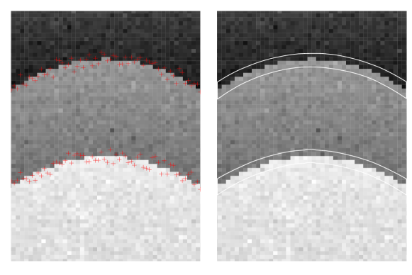
Figure 6: Left picture: Noisy regression function and red crosses indicate the thinned out candidate set of change points. Right picture: Resulting Bonferroni-corrected 95% confidence bands.

4.7 Real data illustration

Finally we apply our method to two $300\times 128$ Gray-scale real-data images, taken by camera by one of the authors. They contain the outline of a rock in front of a gray background. Once, an appropriate ISO–configuration and focus on the rock and once inappropriate ISO–configuration of the camera and no focus at all are employed. In both cases we apply our method to estimate the boundary of the rock and construct 0.95-level uniform confidence sets using $t_{n}=0$ and a naive estimator for the noise-level. Figure 7 contains the results.

The jump-location curve lies mostly inside the constructed confidence band and the width is quite satisfying, although the noise-level of the picture is rather low. This illustration might be representative for more serious applications. For instance, a polar explorer might intend to monitor the height of a glacier in order to analyze the effect of global warming. Due to external effects such as bad weather conditions the pictures of the glacier could be noisy, so that its ridge needs to be estimated. The confidence bands are useful to assess whether the height of the glacier actually decreased.

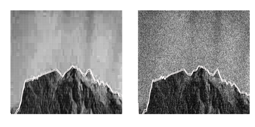
Figure 7: Left: $300\times 128$ Gray-scale picture of a rock taken from a camera with reasonable ISO-configuration and with focus on the rock. Solid lines correspond to the 95%-level confidence band for the noisy picture on the right. Right: $300\times 128$ Gray-scale picture of a rock taken from a camera with inappropriate ISO-configuration and with no focus. Solid lines correspond to the 95%-level confidence band for this noisy picture.

5 Discussion

In this paper we developed methods to construct asymptotic confidence sets for the jump curve in an otherwise smooth two-dimensional regression function, for which to the best of our knowledge no methods were previously available. As a further step, a combination of our results with the issue of edge detection would be desirable. A direct thresholding of the contrast function (6) without prior localization as in (17) seems not to result in confidence sets which decrease at a near optimal rate, so that further methods would be required. An extension of our results to the multivariate setting, especially to three dimensions would also be relevant. Further, images are often observed with blurring, that is, after convolution with a point-spread function. Thus, extensions to a deconvolution setting would also be of practical importance.

6 Outline of proofs

For future reference we collect additional notation that is used in the following.

6.1 Notation

We shall use the following notation. For a vector $\mathbf{z}=(z_{1},z_{2})^{\top}\in\mathbb{R}^{2}$ we denote the coordinate projection onto the $i$th coordinate as $(\mathbf{z})_{i}=z_{i}$ for $i\in\{1,2\}$. Furthermore, we write $\mathbf{z}^{\alpha}=z_{1}^{\alpha_{1}}z_{2}^{\alpha_{2}}$ for $\alpha=(\alpha_{1},\alpha_{2})^{\top}\in\mathbb{N}^{2}$ and

$$f^{(\alpha)}(\mathbf{z})=\frac{\partial^{\alpha_{1}+\alpha_{2}}}{\partial z_{1}^{\alpha_{1}}\partial z_{2}^{\alpha_{2}}}f(\mathbf{z})$$

for a function $f:\mathbb{R}^{2}\to\mathbb{R}$. In particular, $\nabla f(\mathbf{z})=(f^{(1,0)},f^{(0,1)})^{\top}(\mathbf{z})$ and

$$\nabla\nabla^{\top}f(\mathbf{z})=\Big{(}\begin{array}[]{cc}f^{(2,0)}&f^{(1,1)}\\ f^{(1,1)}&f^{(0,2)}\end{array}\Big{)}(\mathbf{z}).$$

We also write $\partial_{z_{i}}f(\mathbf{z})$ for $f^{\mathbf{e_{i}}^{\top}}(\mathbf{z}),$ where $\mathbf{e_{i}}$ is the $i$th canonical unit vector. If $g:X\to Y$ for $X,Y\subset\mathbb{R},$ then we let $\text{epi}(g)=\{(x,y)^{\top}\in X\times Y:g(x)\leq y\}$ be the epigraph of $g$. Let $A\triangle B$ denote the symmetric difference between two sets $A$ and $B$, i.e., for any $A,B\subset\mathbb{R}^{2}$,

$$A\ \triangle\ B=(A\backslash B)\cup(B\backslash A)=(A\cup B)\backslash(A\cap B).$$

Write $\mathbf{z}+A=\{\mathbf{z}+\mathbf{y}:\mathbf{y}\in A\}$ for $\mathbf{z}\in\mathbb{R}^{2}$ and a set $A\subset\mathbb{R}^{2}$. For sequences $a_{n}$ and $b_{n}$ we write $a_{n}\cong b_{n}$ if there exist constants $0<C_{1}<C_{2}$ and $n_{0}\in\mathbb{N}$ such that $C_{1}\leq|a_{n}/b_{n}|\leq C_{2}$ for any $n\geq n_{0}$. Denote by $\|\cdot\|$ a norm on $\mathbb{R}^{2}$ as well as on $\mathbb{R}^{2\times 2}$, where the dimension should be clear from the context. We only assume that the matrix-norm is compatible with the vector-norm, that is $\|\mathbf{A}\mathbf{z}\|\leq\|\mathbf{A}\|\times\|\mathbf{z}\|$ for a matrix $\mathbf{A}$ and a vector $\mathbf{z}$ and that the matrix-norm is submultiplicative, i.e., $\|\mathbf{A}\mathbf{B}\|\leq\|\mathbf{A}\|\times\|\mathbf{B}\|$ for matrices $\mathbf{A},\mathbf{B}$. For a function $f:I\to\mathbb{R}^{i\times j}$ for $i,j\in\{1,2\}$ with $i\geq j$ and $I$ is a compact subinterval of $(0,1)$ we define the uniform-norm as

$$||\,f\,||_{\infty}=\begin{cases}\sup_{x\in I}\ \ |\,f(x)\,|&\mbox{if }i=j=1,\\ \sup_{x\in I}\|f(x)\|&\text{otherwise.}\end{cases}$$

6.2 Rescaling of the contrast function

From now on, we shall always assume that $h$ is so small ($n$ is sufficiently large) that $I\subset[h,1-h]$. Define, for $x\in I$, the set of the rescaled parameters as

$$\begin{split}\tilde{\Theta}_{n,x}=\{w\in\mathbb{R}:\phi(x)+wh\in[h,1-h]\}\times[-\pi/2,\pi/2],\end{split}$$

and for $(x,\psi,w)^{\top}\in I\times\mathbb{R}^{2}$ the rescaled contrast function

$$\hat{\mathbb{M}}_{n}(w,\psi;x)=\hat{\text{M}}_{n}((x,\phi(x)+hw)^{\top};\psi,h)=\hat{\text{M}}_{n}(\mathbf{p}(x)+wh\mathbf{e_{2}};\psi,h),$$ (17)

where $\hat{\text{M}}_{n}$ is given in (6) and $\mathbf{p}(x)=(x,\phi(x))^{\top}$ as well as $\mathbf{e_{2}}=(0,1)^{\top}$. With this, we have for the maximizers

$$\left(\hat{w}_{n}(x),\hat{\psi}_{n}(x)\right)\in\underset{(w,\psi)\in\tilde{\Theta}_{n,x}}{\operatorname{arg}\,\operatorname{max}}\;\hat{\mathbb{M}}_{n}(w,\psi;x)$$ (18)

that $\hat{w}_{n}(x)=\{\hat{\phi}_{n}(x)-\phi(x)\}/h$. The parameter set is denoted by $\Theta_{n}=\bigcup_{x\in I}\{x\}\times\tilde{\Theta}_{n,x}$. We also introduce the deterministic contrast function

$$\mathbb{M}_{n}(w,\psi;x)={\rm E}\{\hat{\mathbb{M}}_{n}(w,\psi;x)\}.$$

6.3 Uniform consistency

In this section we show uniform consistency over $I$ for the maximizers in (18).

Proposition 1.

Under Assumptions 1–4 we have, as $n\to\infty$,

$$||\,\big{(}\hat{w}_{n}(\cdot),(\hat{\psi}_{n}-\psi)(\cdot)\big{)}^{\top}\,||_{\infty}\stackrel{{\scriptstyle\text{P}}}{{\to}}0.$$

For the proof, we make use of the following adaptation of Theorem 5.7 in [27], which is proved in Section LABEL:sec:stochunifconv of the Online Supplement.

Proposition 2.

Assume that $\tilde{\Theta}_{n,x}\subset\mathbb{R}^{d}$ are compact sets and set $\Theta=\cup_{n}\Theta_{n},$ where $\Theta_{n}=\cup_{x\in I}\{x\}\times\tilde{\Theta}_{n,x}$. Let $\hat{f}_{n}:\mathbb{R}^{d}\times I\to\mathbb{R}$ be random functions and let $f:\mathbb{R}^{d}\times I\to\mathbb{R}$ be a deterministic function. Suppose that

$$\sup_{(x,\theta)\in\Theta_{n}}|\hat{f}_{n}(\theta,x)-f(\theta,x)|\stackrel{{\scriptstyle\text{P}}}{{\to}}0,$$ (19)

and that there exists a map $\theta_{0}:I\to\Theta$ such that, for any $\epsilon>0$,

$$\inf_{x\in I}\left[f\{\theta_{0}(x),x\}-\sup_{\theta\in\mathbb{R}^{d}:|\theta-\theta_{0}(x)|\geq\epsilon}f(\theta,x)\right]>0.$$ (20)

Then for any estimator $\hat{\theta}_{n}(x)\in\tilde{\Theta}_{n,x},$ where $x\in I,$ which satisfies

$$\inf_{x\in I}\big{[}\hat{f}_{n}\{\hat{\theta}_{n}(x),x\}-\hat{f}_{n}\{\theta_{0}(x),x\}\big{]}\geq-o_{P}(1)$$

one has $||\,\hat{\theta}_{n}-\theta_{0}\,||_{\infty}\stackrel{{\scriptstyle\text{P}}}{{\to}}0$ as $n\to\infty$.

In order to obtain Proposition 1, in the next two lemmas we check the requirements of Proposition 2. The next lemma determines the limit function for $\hat{\mathbb{M}}_{n}(w,\psi;x)$ and shows that they fulfill the assumption (19).

Lemma 1.

Under Assumptions 1–4, we have that

$$\sup_{(x,w,\psi)^{\top}\in\Theta_{n}}|\hat{\mathbb{M}}_{n}(w,\psi;x)-\mathbb{M}\left(w,\psi;x\right)|=O_{P}(h)+O_{P}\{\ln(n)^{1/2}(nh)^{-1}\},$$

where

$$\mathbb{M}(w,\psi;x)=\tau(x)\int_{\mathbb{H}\{\psi(x)-\psi\}+w(\sin\psi,\cos\psi)^{\top}}K(\mathbf{z})\mathrm{d}\mathbf{z},$$ (21)

and, for any $\psi\in[-\pi,\pi]$, $\mathbb{H}(\psi)=\boldsymbol{\mathscr{R}}_{\psi}\{\mathbb{R}\times[0,\infty)\}$.

Proof of Lemma 1.

Split $\hat{\mathbb{M}}_{n}(w,\psi;x)$ into a smooth-image-related part, a jump-related part and an error-related part as follows

$$\mathbb{M}_{n}(w,\psi;x) =\left(nh\right)^{-2}\sum\limits_{i_{1},i_{2}=1}^{n}m(\mathbf{x_{i_{1},i_{2}}})K[h^{-1}\boldsymbol{\mathscr{R}}_{-\psi}\{\mathbf{p}(x)+hw\mathbf{e_{2}}-\mathbf{x_{i_{1},i_{2}}}\}]$$

$$\quad+\left(nh\right)^{-2}\sum\limits_{i_{1},i_{2}=1}^{n}j_{\tau}\left(\mathbf{x_{i_{1},i_{2}}}\right)K[h^{-1}\boldsymbol{\mathscr{R}}_{-\psi}\{\mathbf{p}(x)+hw\mathbf{e_{2}}-\mathbf{x_{i_{1},i_{2}}}\}]$$

$$\quad+\left(nh\right)^{-2}\sum\limits_{i_{1},i_{2}=1}^{n}\boldsymbol{{\varepsilon}}_{i_{1},i_{2}}K[h^{-1}\boldsymbol{\mathscr{R}}_{-\psi}\{\mathbf{p}(x)+hw\mathbf{e_{2}}-\mathbf{x_{i_{1},i_{2}}}\}]$$

$$=S_{n}(w,\psi;x)+J_{n}(w,\psi;x)+E_{n}(w,\psi;x).$$

Take

$$g_{1}(\mathbf{z})=m(\mathbf{z}),\quad f(\mathbf{z})=4^{-1}\left(\begin{array}[]{cc}K(\mathbf{z})&K(\mathbf{z})\\ K(\mathbf{z})&K(\mathbf{z})\end{array}\right),\quad g_{2}(\mathbf{z})=g_{3}(\mathbf{z})=(1,1)^{\top}.$$

Lemma LABEL:lemma:S_n_term in the Online Supplement with $r_{1}=k=2$, $r_{2}=r_{3}=0$ and $j=1$ states that

$$S_{n}(w,\psi;x)=m\{\mathbf{p}(x)+hw\mathbf{e}_{2}\}\int_{[-1,1]^{2}}K\left(\mathbf{z}\right)\mathrm{d}\mathbf{z}+O(h)+O\{(nh)^{-1}\}=O(h)+O\{(nh)^{-1}\}$$

uniformly over $\Theta_{n}.$ With the same functions $f,g_{2},g_{3}$ as above, one deduces from Lemma LABEL:lemma:J_n_term that

$$J_{n}(w,\psi;x)= \tau(x)\int_{\mathbb{H}\{\psi(x)-\psi\}+w\left(\sin\left(\psi\right),\cos\left(\psi\right)\right)^{\top}}K\left(\mathbf{z}\right)\mathrm{d}\mathbf{z}+O\left(h\right)+O\{(nh)^{-1}\}$$

$$= \mathbb{M}\left(w,\psi;x\right)+O\left(h\right)+O\{(nh)^{-1}\},$$

uniformly over $\Theta_{n}.$ Finally, Lemma LABEL:lemma:E_n_term with the same $f,g_{2},g_{3}$ implies $E_{n}(w,\psi;x)=O_{p}\{\ln(n)^{1/2}(nh)^{-1}\}$ uniform over $\Theta_{n}.$ This concludes the proof of the lemma. ∎

In the next lemma, we rewrite the asymptotic form of the contrast and show that it has a unique well-separated maximum, that is the requirement (20).

Lemma 2.

Under Assumptions 2 and 4, one has that if $\psi(x)-\psi=\pm\pi/2$ then $\mathbb{M}\left(w,\psi;x\right)=0$ for all $w$, while otherwise

$$\mathbb{M}\left(w,\psi;x\right)=-\tau(x)\int_{-1}^{1}K_{1}\left(y\right)\bar{K}_{2}\{a_{x}(\psi)y+b_{x}(w,\psi)\}\mathrm{d}y,$$ (22)

where

$$\bar{K}_{2}\left(y\right)=\int_{-1}^{y}K_{2}\left(t\right)\mathrm{d}t,\quad a_{x}\left(\psi\right)=\tan\{\psi(x)-\psi\},\quad b_{x}\left(w,\psi\right)=w\,\frac{\cos\{\psi(x)\}}{\cos\{\psi(x)-\psi\}}.$$

This implies that for any $\epsilon>0$,

$$\inf_{x\in[0,1]}\Big{\{}\mathbb{M}(0,\psi(x);x)-\sup_{(w,\psi)\in\mathbb{R}^{2}:\ \epsilon\leq\max(|w|,|\psi(x)-\psi|)}\mathbb{M}(w,\psi;x)\Big{\}}>0.$$ (23)

Moreover, $\mathbb{M}(0,\psi(x);x)=\tau(x)$.

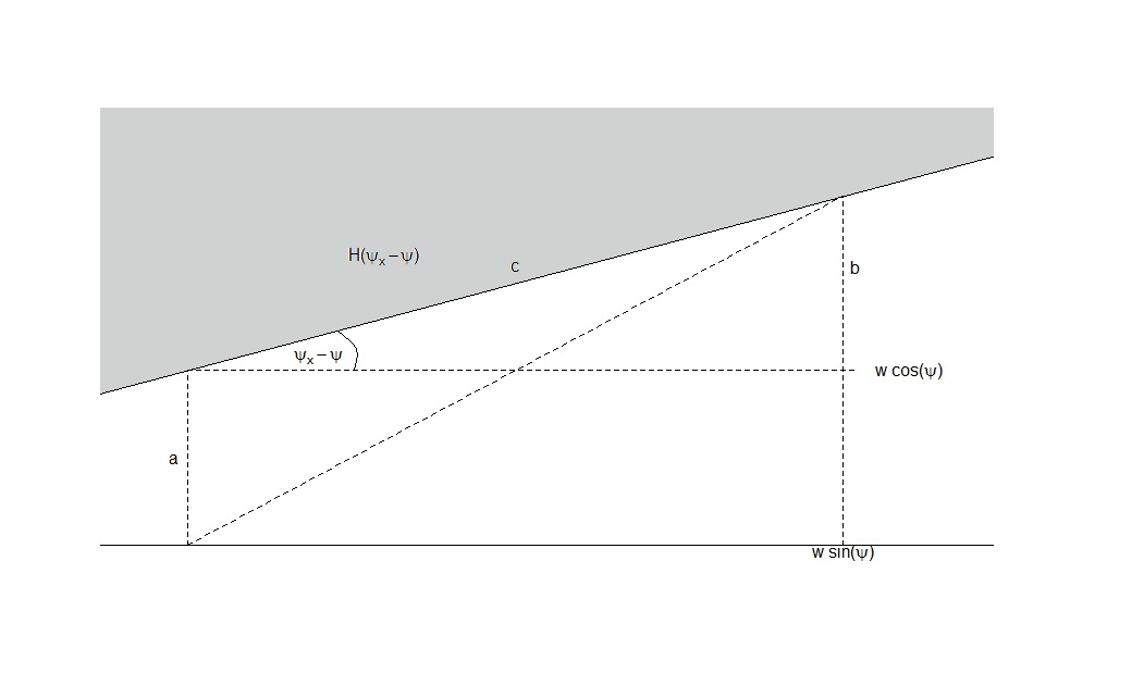
Figure 8: Gray area corresponds to $\mathbb{H}\{\psi(x)-\psi\}$.

Proof of Lemma 2.

If $\psi(x)-\psi=\pi/2$ then $\mathbb{H}\{\psi(x)-\psi\}=(-\infty,0]\times\mathbb{R}$. Since $\int_{\mathbb{R}}K_{2}=\int_{-1}^{1}K_{2}=0$, the statement $\mathbb{M}\left(w,\psi;x\right)=0$ follows from (21), and similarly for $\psi(x)-\psi=-\pi/2$. If $\psi(x)-\psi\not=\pm\pi/2$, we start by showing that

$$\mathbb{H}\{\psi(x)-\psi\}+w\left(\sin\psi,\cos\psi\right)^{\top}=\mathbb{H}\{\psi(x)-\psi\}+w\frac{\cos\{\psi(x)\}}{\cos\{\psi(x)-\psi\}}\,\mathbf{e_{2}},$$

for an illustration see Figure 8. If $w=0$ the assertion is trivial. If $w\not=0$, we need to determine $a$ such that the vector $a\,\mathbf{e_{2}}$ is on the boundary of the set $\mathbb{H}\{\psi(x)-\psi\}+w\left(\sin\psi,\cos\psi\right)^{\top}$; see Figure 8. Setting $c=w\sin\left(\psi\right)/\cos\{\psi(x)-\psi\}$ and $b=c\sin\{\psi(x)-\psi\}$ we get that (see Figure 8)

$$a=w\cos\left(\psi\right)-b=\frac{\cos\left(\psi\right)\cos\{\psi(x)-\psi\}-\sin\left(\psi\right)\sin\{\psi(x)-\psi\}}{\cos\left(\psi(x)-\psi\right)}=\frac{\cos\{\psi(x)\}}{\cos\{\psi(x)-\psi\}}.$$

From (21) we obtain that

$$\mathbb{M}\left(w,\psi;x\right) =\tau(x)\int_{\mathbb{H}\{\psi(x)-\psi\}+w\left(\sin\psi,\cos\psi\right)^{\top}}K\left(\mathbf{z}\right)\mathrm{d}\mathbf{z}$$

$$=\tau(x)\int_{\mathbb{H}\{\psi(x)-\psi\}+b_{x}\left(w,\psi\right)\mathbf{e}_{2}}K_{1}\left(z_{1}\right)K_{2}\left(z_{2}\right)\mathrm{d}z_{1}\mathrm{d}z_{2}$$

$$=\tau(x)\int_{-1}^{1}K_{1}\left(z_{1}\right)\int_{a_{x}(\psi)z_{1}+b_{x}(w,\psi)}^{1}K_{2}\left(z_{2}\right)\mathrm{d}z_{2}\mathrm{d}z_{1}$$

$$=\tau(x)\int_{-1}^{1}K_{1}\left(z_{1}\right)\left[\bar{K}_{2}(1)-\bar{K}_{2}\{a_{x}(\psi)z_{1}+b_{x}(w,\psi)\}\right]\mathrm{d}z_{1}$$

$$=-\tau(x)\int_{-1}^{1}K_{1}\left(z_{1}\right)\bar{K}_{2}\{a_{x}(\psi)z_{1}+b_{x}(w,\psi)\}\mathrm{d}z_{1}.$$

Since $|a_{x}(\psi)y+b_{x}(w,\psi)|\geq 1$ if $|w|\geq 1/{|\cos\{\psi(x)\}|}+1$ for all $y\in[-1,1]$ and $\psi\in[-\pi/2,\pi/2]$, $\mathbb{M}\left(w,\psi;x\right)$ vanishes outside a compact set of values of $w$ and $x$.

Turning to (23), if we show that it holds for individual $x$, then since the supremum in (23) can be taken over a single compact set, we have that the left-hand side of (23) is a continuous function in $x$ which is positive for any $x\in[0,1]$. Hence, the infimum over $x\in[0,1]$ is still positive.

To show that (23) holds for individual $x$, we observe that $-\bar{K}_{2}(0)=1$, $-\bar{K}_{2}(y)<1$ if $y\not=0$, and $\bar{K}_{2}(y)=0$ if $|y|\geq 1$ by Assumption 4. Since $\mathbb{M}\left(w,\psi;x\right)$ is continuous in $w$ and $\psi$, as can also be seen from (21), it is enough to show that $(0,\psi(x))$ is the unique maximizer of $\mathbb{M}(w,\psi;x)$. But this is immediate from (22) and the above properties of $\bar{K}_{2}$ and the positivity of $K_{1}$, since if $(w,\psi)\not=(0,\psi(x))$, there is at most a single value of $z_{1}$ for which $a_{x}(\psi)z_{1}+b_{x}(w,\psi)=0$ and hence $-\bar{K}_{2}\{a_{x}(\psi)z_{1}+b_{x}(w,\psi)\}=1$. ∎

Proof of Proposition 1.

The uniform consistency of the estimates $\hat{w}_{n}$ and $\hat{\psi}_{n}$ is immediate from Proposition 2, as Lemma 1 and Lemma 2 provide the necessary assumptions. ∎

6.4 Rate of convergence: Proof of Theorem 1

To prove the theorems in the main part we start with a simple linearization. By the Mean Value Theorem, we have that

$$\nabla\hat{\mathbb{M}}_{n}\left(0,\psi(x);x\right) =\nabla\hat{\mathbb{M}}_{n}\left(0,\psi(x);x\right)-\nabla\hat{\mathbb{M}}_{n}\big{(}\hat{w}_{n}(x),\hat{\psi}_{n}(x);x\big{)}$$

$$=-\int_{0}^{1}\nabla\nabla^{\top}\hat{\mathbb{M}}_{n}\big{(}t\hat{w}_{n}(x),\psi(x)+t\{\hat{\psi}_{n}(x)-\psi(x)\};x\big{)}\mathrm{d}t\ (\hat{w}_{n}(x),\hat{\psi}_{n}(x)-\psi(x))^{\top},$$

since $\nabla\hat{\mathbb{M}}_{n}\left(\hat{w}_{n}(x),\hat{\psi}_{n}(x);x\right)=0$. This implies

$$\left(\hat{w}_{n}(x),\hat{\psi}_{n}(x)-\psi(x)\right)^{\top}=-\hat{\mathbf{H}}^{-1}_{n}(x)\ \nabla\hat{\mathbb{M}}_{n}\left(0,\psi(x);x\right),$$ (24)

where

$$\hat{\mathbf{H}}_{n}(x)=\int_{0}^{1}\nabla\nabla^{\top}\hat{\mathbb{M}}_{n}\left(t\hat{w}_{n}(x),\psi(x)+t\{\hat{\psi}_{n}(x)-\psi(x)\};x\right)\mathrm{d}t,$$

and the existence of the inverse of the Hessian matrix $\hat{\mathbf{H}}_{n}(x)$ uniformly in $x\in I$ for large $n$ and with high probability follows from Lemma 4 below.

Similarly as in (24), for the rescaled maximizers of the deterministic contrast function, i.e.,

$$(w_{n}(x),\psi_{n}(x))\in\underset{(w,\psi)^{\top}\in\tilde{\Theta}_{n,x}}{\operatorname{arg}\,\operatorname{max}}\;\mathbb{M}_{n}(w,\psi,x),$$

we have that

$$\left(w_{n}(x),\psi_{n}(x)-\psi(x)\right)^{\top}=-{\mathbf{H}}^{-1}_{n}(x)\ \nabla\mathbb{M}_{n}\left(0,\psi(x);x\right),$$ (25)

where $w_{n}(x)=\{\phi_{n}(x)-\phi(x)\}/h$ and the deterministic Hessian matrix is given by

$${\mathbf{H}}_{n}(x)=\int_{0}^{1}\nabla\nabla^{\top}\mathbb{M}_{n}\left(t\,w_{n}(x),\psi(x)+t\{\psi_{n}(x)-\psi(x)\};x\right)\mathrm{d}t.$$

By means of (25), we can decompose the representation in (24) into a stochastic part (or score part), a bias part and a remainder term as follows:

$$\left(\hat{w}_{n}(x),\hat{\psi}_{n}(x)-\psi(x)\right)^{\top} =\hat{\mathbf{H}}^{-1}_{n}(x)\boldsymbol{\mathscr{S}}_{n}^{\phi,\psi}(0,\psi(x);x)-{\mathbf{H}}^{-1}_{n}(x)\ \boldsymbol{\mathscr{B}}_{n}^{\phi,\psi}(x)+R_{n}^{\phi,\psi}(x),$$ (26)

where

$$\begin{split}\boldsymbol{\mathscr{S}}_{n}^{\phi,\psi}(w,\psi;x)&=(\boldsymbol{\mathscr{S}}_{n}^{\phi}(w,\psi;x),\boldsymbol{\mathscr{S}}_{n}^{\psi}(w,\psi;x))^{\top}=-\{\nabla\hat{\mathbb{M}}_{n}\left(w,\psi;x\right)-\nabla\mathbb{M}_{n}\left(w,\psi;x\right)\},\\ \boldsymbol{\mathscr{B}}_{n}^{\phi,\psi}(x)&=(\boldsymbol{\mathscr{B}}_{n}^{\phi}(x),\boldsymbol{\mathscr{B}}_{n}^{\psi}(x))^{\top}=\nabla\mathbb{M}_{n}(0,\psi(x);x),\\ R_{n}^{\phi,\psi}(x)&=\{\mathbf{H}^{-1}_{n}(x)-\hat{\mathbf{H}}^{-1}_{n}(x)\}\boldsymbol{\mathscr{B}}_{n}^{\phi,\psi}(x).\end{split}$$

Note that by (22) we have $\tau(x)=\mathbb{M}(0,\psi(x);x)$ and $\hat{\tau}_{n}(x)=\hat{\mathbb{M}}_{n}(\hat{w}_{n}(x),\hat{\psi}_{n}(x);x)$ such that by the Mean Value Theorem as well as adding and subtracting $\mathbb{M}_{n}(0,\psi(x);x)$, one has

$$\begin{split}\hat{\tau}_{n}(x)-\tau(x)&=\hat{\mathbb{M}}_{n}(0,\psi(x);x)-\mathbb{M}(0,\psi(x);x)\\ &\quad+(\hat{w}_{n}(x),\hat{\psi}_{n}(x)-\psi(x))\int_{0}^{1}\nabla\hat{\mathbb{M}}_{n}\left(t\hat{w}_{n}(x),\psi(x)+t\{\hat{\psi}_{n}(x)-\psi(x)\};x\right)\mathrm{d}t\\ &=\boldsymbol{\mathscr{S}}_{n}^{\tau}(0,\psi(x);x)+\boldsymbol{\mathscr{B}}_{n}^{\tau}(x)+R_{n}^{\tau}(x),\end{split}$$ (27)

where

$$\begin{split}\boldsymbol{\mathscr{S}}_{n}^{\tau}(w,\psi;x)&=\hat{\mathbb{M}}_{n}(w,\psi;x)-\mathbb{M}_{n}(w,\psi;x),\\ \boldsymbol{\mathscr{B}}_{n}^{\tau}(x)&=\mathbb{M}_{n}(0,\psi(x);x)-\mathbb{M}(0,\psi(x);x),\\ R_{n}^{\tau}(x)&=(\hat{w}_{n}(x),\hat{\psi}_{n}(x)-\psi(x))\int_{0}^{1}\nabla\hat{\mathbb{M}}_{n}\left(t\hat{w}_{n}(x),\psi(x)+t\{\hat{\psi}_{n}(x)-\psi(x)\};x\right)\mathrm{d}t.\end{split}$$

6.5 Asymptotic bias

Lemma 3.

One has $\nabla\mathbb{M}_{n}(w,\psi;x)={\rm E}\{\nabla\hat{\mathbb{M}}_{n}(w,\psi;x)\}$ for any $(x,w,\psi)\in\Theta_{n}$. Moreover, under Assumptions 2 and 4 we have that

$$\sup_{x\in I}\|\boldsymbol{\mathscr{B}}_{n}^{\phi}\|=O(h^{2})+O\{(nh)^{-1}\}.$$

If in addition Assumption 5 is fulfilled, then

$$\sup_{x\in I}\|\boldsymbol{\mathscr{B}}_{n}^{\psi}\|=O(h^{2})+O\{(nh)^{-1}\},\quad\sup_{x\in I}\|\boldsymbol{\mathscr{B}}_{n}^{\tau}\|=O(h^{2})+O\{(nh)^{-1}\}.$$

The constants in the remainder terms depend only on the Lipschitz constants of $K,m,\phi$ and $\psi$ as well as on $||\,\tau\,||_{\infty}$. In particular, if Assumption 3 is satisfied, then

$$\sup_{x\in I}\ \max\{\|\boldsymbol{\mathscr{B}}_{n}^{\phi}(x)\|,\|\boldsymbol{\mathscr{B}}_{n}^{\psi}(x)\|,\|\boldsymbol{\mathscr{B}}_{n}^{\tau}(x)\|\}=O\{(nh)^{-1}\}.$$

The proof of this lemma is provided in Section LABEL:sec:asymbias of the Online Supplement. The bias consists of a smoothing bias of order $O(h^{2}),$ and a discretization bias of order $O\{(nh)^{-1}\}$, which dominates the order of the bias in case of undersmoothing, that is under Assumption 3.

6.6 Convergence of the Hessian matrix

Lemma 4.

Under Assumptions 1–4, we have, as $n\to\infty$,

$$||\,\hat{\mathbf{H}}_{n}-\mathbf{H}\,||_{\infty}\stackrel{{\scriptstyle\text{P}}}{{\to}}0\quad\text{and}\quad||\,\mathbf{H}_{n}-\mathbf{H}\,||_{\infty}\to 0,$$

where $\mathbf{H}(x)={\rm diag}\{V_{\phi}^{H}(x),V_{\psi}^{H}(x)\}$ and $V_{\phi}^{H}(x)$ as in Theorem 2, while

$$V_{\psi}^{H}(x)=\tau(x)K_{2}^{(1)}(0)\int_{-1}^{1}y^{2}K_{1}(y)\mathrm{d}y.$$

The proof of Lemma 4 is provided in Section LABEL:sec:convhessian of the Online Supplement. Note that the limit matrix $\mathbf{H}$ corresponds to the Hessian matrix of the asymptotic criterion function $\mathbb{M}$ at the parameters $w=0$ and $\psi=\psi(x)$. Furthermore, we only need the uniform consistency in Lemma 4 to derive the proof of Theorem 1 and 2. However, for the proof of Theorem 3 we need the uniform convergence even with an explicit rate of convergence.

Proposition 3.

Under Assumptions 1–4, we have that

$$\sup_{x\in I}\|\boldsymbol{\mathscr{S}}_{n}^{\phi,\psi}(0,\psi(x);x)\| =O_{P}\{(\ln n)^{1/2}/(nh)\},$$

$$\sup_{x\in I}\|\boldsymbol{\mathscr{S}}_{n}^{\tau}(0,\psi(x);x)\| =O_{P}\{(\ln n)^{1/2}/(nh)\}.$$

The proof of this proposition is provided in Section LABEL:sec:asympscore of the Online Supplement. $\Box$

Proof of Theorem 1.

Lemma 4 implies that $\hat{\mathbf{H}}^{-1}_{n}$ is almost surely a stochastically bounded matrix-valued sequence uniformly in $x$. Hence, in combination with Lemma 3 deduce

$$\sup_{x\in I}\|\hat{\mathbf{H}}^{-1}_{n}(x)\ \boldsymbol{\mathscr{B}}_{n}^{\phi,\psi}(x)\|=O_{P}(h^{2})+O_{P}\{(nh)^{-1}\}$$ (28)

as well as

$$\sup_{x\in I}\|R_{n}^{\phi,\psi}(x)\|=o_{P}(h^{2})+o_{P}\{(nh)^{-1}\}.$$ (29)

Next, Slutzky’s Lemma and Proposition 3 imply

$$\sup_{x\in I}\|\hat{\mathbf{H}}^{-1}_{n}(x)\ \boldsymbol{\mathscr{S}}_{n}^{\phi,\psi}(0,\psi(x);x)\|=O_{P}\{(\ln n)^{1/2}/(nh)\}.$$

From (26) it immediately follows by combining the three latter displays that

$$||\,(\hat{w}_{n},\hat{\psi}_{n}-\psi)^{\top}\,||_{\infty}=O_{P}\{(\ln n)^{1/2}/{(nh)}\}+O_{P}(h^{2})=O_{P}\{(\ln n)^{1/2}/(nh)\},$$

where the last equation is due to Assumption 3. Note that Assumption 5 is only needed for the bias of the slope in (28).

The uniform rate of convergence for $\hat{\tau}_{n}$ now follows with a similar argument. Indeed, due to representation (27) and Lemma 3 and Proposition 3 it suffices to show that

$$||\,R_{n}^{\tau}\,||_{\infty}=o_{P}\{(nh)^{-1}\}.$$ (30)

Since we verified above that $||\,\hat{w}_{n},(\hat{\psi}_{n}-\psi)\,||_{\infty}=O_{P}\{(\ln n)^{1/2}/(nh)\}$ holds, we only need to show that

$$\sup_{x\in I}\|f(\hat{w}_{n}(x),\hat{\psi}_{n}(x);x)\|=o_{P}\{(\ln n)^{-1/2}\},$$

where we abbreviate

$$f(w,\psi;x)=\int_{0}^{1}\nabla\hat{\mathbb{M}}_{n}\left(tw,\psi(x)+t\{\psi-\psi(x)\};x\right)\mathrm{d}t.$$

By the Mean Value Theorem (differentiating under the integral), Lemma 4 and since $\hat{\mathbf{H}}_{n}$ is uniformly bounded,

$$\begin{split}\sup_{x\in I}\|f(\hat{w}_{n}(x),\hat{\psi}_{n}(x);x)-f(0,\psi(x);x)\|&\leq\|\hat{\mathbf{H}}_{n}\|\sup_{x\in I}|\big{(}\hat{w}_{n}(x),\hat{\psi}_{n}(x)-\psi(x)\big{)}^{\top}|\\ &=O_{P}\{(\ln n)^{1/2}/(nh)\}=o_{P}\{(\ln n)^{-1/2}\},\end{split}$$ (31)

where the last equation is justified by Assumption 3. Note that

$$f(0,\psi(x);x)=\nabla\hat{\mathbb{M}}_{n}(0,\psi(x);x)=\boldsymbol{\mathscr{S}}_{n}^{\phi,\psi}(0,\psi(x);x)-\boldsymbol{\mathscr{B}}_{n}^{\phi,\psi}(x).$$

Hence, due to Lemma 3, Proposition 3 and the triangle inequality

$$\sup_{x\in I}\|f(0,\psi(x);x)\|=O_{P}\{(\ln n)^{1/2}/(nh)\}=o_{P}\{(\ln n)^{-1/2}\},$$ (32)

so that $\sup_{x\in I}\|f(\hat{w}_{n}(x),\hat{\psi}_{n}(x);x)\|=o_{P}\{(\ln n)^{-1/2}\}$ follows by (31) and (32) by using the triangle inequality. ∎

6.7 Asymptotic normality: Proof of Theorem 2

We first establish the asymptotic normality of the score.

Lemma 5.

Under Assumptions 1, 3 and 4 we have that, for any $x\in I$, as $n\to\infty$,

$$nh\left(\begin{array}[]{c}\boldsymbol{\mathscr{S}}_{n}^{\phi}(0,\psi(x);x)\\ \boldsymbol{\mathscr{S}}_{n}^{\psi}(0,\psi(x);x)\\ \boldsymbol{\mathscr{S}}_{n}^{\tau}\ \ (0,\psi(x);x)\end{array}\right)\rightsquigarrow\mathcal{N}_{3}[\mathbf{0},\sigma^{2}{\rm diag}(V_{\phi}^{S}(x),V_{\psi}^{S},V_{\tau}^{S})],$$

where $V_{\phi}^{S}$ is as in Theorem 2 and

$$V_{\psi}^{S} =\int_{-1}^{1}\Big{[}\int_{-1}^{1}\{K_{1}(z_{1})K_{2}^{(1)}(z_{2})z_{1}-K_{1}^{(1)}(z_{1})K_{2}(z_{2})z_{2}\}^{2}\mathrm{d}z_{1}\Big{]}\mathrm{d}z_{2},\quad V_{\tau}^{S}=\int_{[-1,1]^{2}}\{K(\mathbf{z})\}^{2}\mathrm{d}\mathbf{z}.$$

Section LABEL:sec:asympscore of the Online Supplement contains the proof of this lemma. Theorem 2 now follows immediately from the following more general theorem, since $\hat{w}_{n}(x)=\{\hat{\phi}_{n}(x)-\phi(x)\}/h$ as well as $w_{n}(x)=\{\phi_{n}(x)-\phi(x)\}/h$.

Theorem 4.

Under Assumptions 1–4, one has, as $n\to\infty$,

$$nh\,\left(\begin{array}[]{c}\hat{w}_{n}(x)-w_{n}(x)\\ \hat{\psi}_{n}(x)-\psi_{n}(x)\\ \hat{\tau}_{n}(x)-\tau_{n}(x)\end{array}\right)\rightsquigarrow\mathcal{N}_{3}[\mathbf{0},\sigma^{2}\,\Sigma(x)],$$

where $\Sigma(x)={\rm diag}[V_{\phi}^{S}(x)/\{V_{\phi}^{H}(x)\}^{2},V_{\psi}^{S}/\{V_{\psi}^{H}(x)\}^{2},V_{\tau}^{S}]$.

Proof of Theorem 4.

From (24) and (25), we obtain that

$$nh\,\left(\hat{w}_{n}(x)-w_{n}(x),\hat{\psi}_{n}(x)-\psi_{n}(x)\right)^{\top}=\hat{\mathbf{H}}^{-1}_{n}(x)\ nh\boldsymbol{\mathscr{S}}_{n}^{\phi,\psi}(0,\psi(x);x)+nhR_{n}^{\phi,\psi}(x).$$

Now, by the Mean Value Theorem one has that

$$\tau_{n}(x)-\tau(x) =\mathbb{M}_{n}(w_{n}(x),\psi_{n}(x);x)-\mathbb{M}(0,\psi(x);x)$$

$$=\boldsymbol{\mathscr{B}}_{n}^{\tau}(x)+(w_{n}(x),\psi_{n}(x)-\psi(x))\int_{0}^{1}\nabla\mathbb{M}_{n}\left(tw,\psi(x)+t\{\psi-\psi(x)\};x\right)\mathrm{d}t$$

$$=\boldsymbol{\mathscr{B}}_{n}^{\tau}(x)+R_{n,2}^{\tau}(x).$$

With this, (27) and the first display of this proof, we have

$$nh\,\left(\begin{array}[]{c}\hat{w}_{n}(x)-w_{n}(x)\\ \hat{\psi}_{n}(x)-\psi_{n}(x)\\ \hat{\tau}_{n}(x)-\tau_{n}(x)\end{array}\right)= nh\left(\begin{array}[]{c}\hat{\mathbf{H}}^{-1}_{n}(x)\ \boldsymbol{\mathscr{S}}_{n}^{\phi,\psi}(0,\psi(x);x)\\ \boldsymbol{\mathscr{S}}_{n}^{\tau}(0,\psi(x);x)\end{array}\right)+nh\left(\begin{array}[]{c}R_{n}^{\phi,\psi}(x)\\ R_{n}^{\tau}(x)-R_{n,2}^{\tau}(x)\end{array}\right).$$ (40)

On the one hand, the first term is asymptotically normally distributed with covariance matrix $\Sigma$ as in the assumption, since by Lemmas 4 and 5 and Slutzky’s Lemma one has, for all $x\in(0,1)$,

$$\big{(}\Sigma(x)\big{)}_{1:2,1:2}=\sigma^{2}\,\hat{\mathbf{H}}^{-2}(x){\rm diag}\{V_{\phi}^{S}(x),V_{\psi}^{S}\},$$

where $(\Sigma(x))_{1:2,1:2}$ is the matrix given consisting of the first two columns or first two rows of $\Sigma(x)$. On the other hand, the second term on the right-hand side (40) is $o_{P}(1)$ by (29) and (30), whereas one can show $R_{n,2}^{\tau}(x)=o_{p}\{(nh)^{-1}\}$ similar as (30). This concludes the proof of Theorem 4. ∎

6.8 Uniform confidence bands: Proof of Theorem 3

For the proof of Theorem 3 we require rates of convergence of the normalized estimators of the Hessian matrix.

Lemma 6.

Under Assumptions 1–4 we have that

$$||\,V_{\widehat{\phi}}^{H}-V_{\phi}^{H}\,||_{\infty}=O_{P}(h)+O_{P}\{\sqrt{\ln(n)}/{(nh)}\},\quad||\,V_{\widehat{\phi}}^{S}-V_{\phi}^{S}\,||_{\infty}=O_{P}\{\sqrt{\ln(n)}/{(nh)}\},$$

$$||\,V_{\widehat{\psi}}^{H}-V_{\psi}^{H}\,||_{\infty}=O_{P}(h)+O_{P}\{\sqrt{\ln(n)}/{(nh)}\},\quad||\,\mathbf{\hat{H}}_{n}^{-1}-\mathbf{H}^{-1}\,||_{\infty}=O_{P}(h)+O_{P}\{\sqrt{\ln(n)}/{(nh)}\}.$$

Here, $V_{\widehat{\psi}}^{H}=\hat{\tau}_{n}(x)K_{2}^{(1)}(0)\int_{-1}^{1}y^{2}K_{1}(y)\mathrm{d}y.$

The proof is provided in Section LABEL:sec:rate_of_conhessian of the Online Supplement.

Next we extend our notation by incorporating the following definition. The Lévy-concentration function of a random variable $X$ is given, for all $\zeta\geq 0$, by

$$\mathbb{L}(X,\zeta)=\sup_{x\in\mathbb{R}}\Pr(|X-x|\leq\zeta).$$

We introduce the normalized score process

$$\begin{split}Z^{\varepsilon}_{n,\phi}(x)&=\sigma^{-1}\{V_{\phi}^{S}(x)\}^{-1/2}\ nh\boldsymbol{\mathscr{S}}_{n}^{\phi}(0,\psi(x);x).\\ \end{split}$$ (41)

It easily follows from Lemma LABEL:lemma:first_deriv_empcrit in the Online Supplement that

$$\boldsymbol{\mathscr{S}}_{n}^{\phi}(0,\psi(x);x) =\partial_{w}\{\hat{\mathbb{M}}_{n}(0,\psi(x);x)-\mathbb{M}_{n}(0,\psi(x);x)\}$$

$$=(n^{2}h^{2})^{-1}\sum\limits_{i_{1},i_{2}=1}^{n}\boldsymbol{{\varepsilon}}_{i_{1},i_{2}}\langle\,(\nabla K)\{h^{-1}\boldsymbol{\mathscr{R}}_{-\psi(x)}(\mathbf{p}(x)-\mathbf{x_{i_{1},i_{2}}})\},(\sin\psi(x),\cos\psi(x))^{\top}\,\rangle,$$

such that

$$Z^{\varepsilon}_{n,\phi}(x) =\frac{1}{nh\sqrt{V_{\phi}^{S}(x)}\sigma}\sum\limits_{i_{1},i_{2}=1}^{n}\boldsymbol{{\varepsilon}}_{i_{1},i_{2}}\langle\,(\nabla K)\{h^{-1}\boldsymbol{\mathscr{R}}_{-\psi(x)}(x,\phi(x))^{\top}-\mathbf{x_{i_{1},i_{2}}})\},(\sin\psi(x),\cos\psi(x))^{\top}\,\rangle.$$

The score process in (11) can be obtained from the latter display by replacing the actual parameters $(\phi,\psi)$ by their estimates $(\hat{\phi}_{n},\hat{\psi}_{n})$ and the noise of the observations $\boldsymbol{{\varepsilon}}_{i_{1},i_{2}}/\sigma$ by the sequence $\xi_{i_{1},i_{2}}$. Similarly to (12) we set

$${\mathscr{Z}}_{n,\phi}^{\varepsilon}=||\,Z^{\varepsilon}_{n,\phi}\,||_{\infty}.$$

Lemma 7.

Under Assumptions 1–4 the following statements are valid.

• By possibly enriching the probability space, one has

  $$|{\mathscr{Z}}_{n,\phi}^{\varepsilon}-\mathscr{Z}^{\xi}_{n,\widehat{\phi}}|=O_{P}\Big{\{}\frac{(\ln n)^{1/2}}{n^{1/2}h}\Big{\}}.$$

• One has $\mathscr{Z}^{\xi}_{n,\widehat{\phi}}=O_{P}\{(\ln n)^{1/2}\}$ and for any sequence $\delta_{n}=o\{(\ln n)^{-1/2}\}$, one has $\mathbb{L}(\mathscr{Z}^{\xi}_{n,\widehat{\phi}},\delta_{n})=o(1)$.

• Moreover, $q_{1-\alpha}(\mathscr{Z}^{\xi}_{n,\widehat{\phi}})\cong(\ln\,n)^{1/2}.$

The proof is given in Section LABEL:sec:gauss_approx_phi_psi of the Online Supplement.

Proof of Theorem 3.

Set $\hat{d}_{n}=\hat{\sigma}_{n}q_{1-\alpha}(\mathscr{Z}^{\xi}_{n,\widehat{\phi}})$. Recall that for $\mathbf{z}=(z_{1},z_{2})^{\top}\in\mathbb{R}^{2}$ we write $(\mathbf{z})_{i}=z_{i}$ for $i\in\{1,2\}$. From (26) we obtain that

$$\Pr\Big{[}\sup_{x\in I}\Big{|}\frac{V_{\widehat{\phi}}^{H}(x)\{\hat{\phi}_{n}(x)-\phi(x)\}}{\{V_{\widehat{\phi}}^{S}(x)\}^{1/2}} \Big{|}\geq{\hat{d}_{n}(1+t_{n})}/{n}\Big{]}$$

$$=\Pr\Big{[}\sup_{x\in I}\Big{|}\frac{V_{\widehat{\phi}}^{H}(x)}{\{V_{\widehat{\phi}}^{S}(x)\}^{1/2}}\,nh\Big{[}\hat{\mathbf{H}}^{-1}_{n}(x)\{\boldsymbol{\mathscr{S}}_{n}^{\phi,\psi}(0,\psi(x);x)+\boldsymbol{\mathscr{B}}_{n}^{\phi,\psi}(x)\}\Big{]}_{1}\Big{|}\geq\hat{d}_{n}(1+t_{n})\Big{]}$$

$$\leq\Pr\Big{[}\sup_{x\in I}\Big{|}\frac{V_{\widehat{\phi}}^{H}(x)}{\{V_{\widehat{\phi}}^{S}(x)\}^{1/2}}\,nh\Big{[}\hat{\mathbf{H}}^{-1}_{n}(x)\,\boldsymbol{\mathscr{S}}_{n}^{\phi,\psi}(0,\psi(x);x)\Big{]}_{1}\Big{|}\geq\hat{d}_{n}\Big{]}$$

$$\quad+\Pr\Big{[}\sup_{x\in I}\Big{|}\frac{V_{\widehat{\phi}}^{H}(x)}{\{V_{\widehat{\phi}}^{S}(x)\}^{1/2}}\Big{[}\hat{\mathbf{H}}^{-1}_{n}(x)\ nh\boldsymbol{\mathscr{B}}_{n}^{\phi,\psi}(x)\Big{]}_{1}\Big{|}\geq t_{n}\hat{d}_{n}\Big{]}.$$

From the last statement of Lemma 7 and the assumption on $t_{n}$ we deduce that $t_{n}\hat{d}_{n}\to\infty$ as $n\to\infty$. Hence, by using Lemmas 3 and 6 the second term in the preceding display can be bounded by

$$\Pr\Big{[}\sup_{x\in I}\Big{|}\frac{V_{\widehat{\phi}}^{H}(x)}{\{V_{\widehat{\phi}}^{S}(x)\}^{1/2}}\Big{[}\hat{\mathbf{H}}^{-1}_{n}(x)\ nh\boldsymbol{\mathscr{B}}_{n}^{\phi,\psi}(x)\Big{]}_{1}\Big{|}\geq t_{n}\hat{d}_{n}\Big{]}=o(1).$$

Recalling the notation in (41), the first term can be estimated by

$$\begin{split}\Pr\Big{[}\sup_{x\in I}&\Big{|}\frac{V_{\widehat{\phi}}^{H}(x)}{\{V_{\widehat{\phi}}^{S}(x)\}^{1/2}}nh\Big{[}\hat{\mathbf{H}}^{-1}_{n}(x)\boldsymbol{\mathscr{S}}_{n}^{\phi,\psi}(0,\psi(x);x)\Big{]}_{1}\Big{|}\geq\hat{d}_{n}\Big{]}\\ &\leq\Pr\Big{[}\sup_{x\in I}|\,\Big{[}\Big{[}\frac{V_{\widehat{\phi}}^{H}(x)}{\{V_{\widehat{\phi}}^{S}(x)\}^{1/2}}\hat{\mathbf{H}}^{-1}_{n}(x)-\frac{V_{\phi}^{H}(x)}{\{V_{\phi}^{S}(x)\}^{1/2}}\mathbf{H}^{-1}(x)\Big{]}\ nh\,\boldsymbol{\mathscr{S}}_{n}^{\phi,\psi}(0,\psi(x);x)\Big{]}_{1}\,|\geq\ln(n)^{-1}\ \Big{]}\\ &\quad+\Pr\Big{[}{\mathscr{Z}}_{n,\phi}^{\varepsilon}\geq\{\hat{d}_{n}-\ln(n)^{-1}\}/\sigma\Big{]}.\end{split}$$ (42)

Lemma 6 implies that

$$||\,({V_{\widehat{\phi}}^{H}}/{\sqrt{V_{\widehat{\phi}}^{S}}})\hat{\mathbf{H}}^{-1}_{n}-(V_{\phi}^{H}/\sqrt{V_{\phi}^{S}})\mathbf{H}^{-1}\,||_{\infty}=O_{P}(h)+O_{P}\{(\ln n)^{1/2}/{(nh)}\},$$

and together with Proposition 3 the first term in (42) can be bounded by

$$O_{P}\{(\ln n)^{3/2}h\}+O_{P}\{(\ln n)^{2}/nh\}=o_{P}(1),$$

due to Assumption 3. As for the second term, plugging in $\hat{d}_{n}=\hat{\sigma}_{n}q_{1-\alpha}(\mathscr{Z}^{\xi}_{n,\widehat{\phi}})$ gives

$$\Pr\Big{[}{\mathscr{Z}}_{n,\phi}^{\varepsilon}\geq \{\hat{\sigma}_{n}q_{1-\alpha}(\mathscr{Z}^{\xi}_{n,\widehat{\phi}})-\ln(n)^{-1}\}/\sigma\Big{]}$$

$$\leq\Pr\{{\mathscr{Z}}_{n,\phi}^{\varepsilon}-\mathscr{Z}^{\xi}_{n,\widehat{\phi}}\geq\ln(n)^{-1}/\sigma\}+\Pr[\mathscr{Z}^{\xi}_{n,\widehat{\phi}}\geq\{\hat{\sigma}_{n}q_{1-\alpha}(\mathscr{Z}^{\xi}_{n,\widehat{\phi}})-2\,\ln(n)^{-1}\}/\sigma]$$

$$\leq \,o(1)+\Pr\Big{\{}\mathscr{Z}^{\xi}_{n,\widehat{\phi}}\geq q_{1-\alpha}(\mathscr{Z}^{\xi}_{n,\widehat{\phi}})\hat{\sigma}_{n}/\sigma\Big{\}}+\mathbb{L}\big{(}\mathscr{Z}^{\xi}_{n,\widehat{\phi}},2\,\ln(n)^{-1}/\sigma\big{)}$$

by using the first part of Lemma 7 together with the choice of $h$, and the definition of the Lévy-concentration function. The last term in this display is $o(1)$ by using the second part of Lemma 7. Finally, observe that

$$\Pr\Big{\{}\mathscr{Z}^{\xi}_{n,\widehat{\phi}}\geq q_{1-\alpha}(\mathscr{Z}^{\xi}_{n,\widehat{\phi}})\hat{\sigma}_{n}/\sigma\Big{\}} \leq\Pr\Big{\{}\mathscr{Z}^{\xi}_{n,\widehat{\phi}}\geq q_{1-\alpha}(\mathscr{Z}^{\xi}_{n,\widehat{\phi}})\Big{\}}+\Pr\Big{\{}\big{|}\mathscr{Z}^{\xi}_{n,\widehat{\phi}}-q_{1-\alpha}(\mathscr{Z}^{\xi}_{n,\widehat{\phi}})\big{|}\leq\big{|}\hat{\sigma}_{n}/\sigma-1\big{|}q_{1-\alpha}(\mathscr{Z}^{\xi}_{n,\widehat{\phi}})\Big{\}}$$

$$\leq\Pr\big{\{}\mathscr{Z}^{\xi}_{n,\widehat{\phi}}\geq q_{1-\alpha}(\mathscr{Z}^{\xi}_{n,\widehat{\phi}})\big{\}}+\mathbb{L}\big{(}\mathscr{Z}^{\xi}_{n,\widehat{\phi}},s_{n}q_{1-\alpha}(\mathscr{Z}^{\xi}_{n,\widehat{\phi}})\,\big{)}+\Pr(|\hat{\sigma}_{n}/\sigma-1|\geq s_{n})$$

$$=\Pr\Big{\{}\mathscr{Z}^{\xi}_{n,\widehat{\phi}}\geq q_{1-\alpha}(\mathscr{Z}^{\xi}_{n,\widehat{\phi}})\Big{\}}+o(1),$$

where $s_{n}$ is as in the assumption of the theorem and where we used the second statement of Lemma 7 together with the third statement of Lemma 7 to obtain $s_{n}q_{1-\alpha}(\mathscr{Z}^{\xi}_{n,\widehat{\phi}})=o\{(\ln n)^{-1/2}\}$.

Summarizing, we obtain that

$$\Pr\Bigg{[}\sup_{x\in I}\Big{|}\frac{V_{\widehat{\phi}}^{H}(x)\{\hat{\phi}_{n}(x)-\phi(x)\}}{\{V_{\widehat{\phi}}^{S}(x)\}^{1/2}}\Big{|}\geq{\hat{d}_{n}(1+t_{n})}/{n}\Bigg{]}\leq\Pr\big{\{}\mathscr{Z}^{\xi}_{n,\widehat{\phi}}\geq q_{1-\alpha}(\mathscr{Z}^{\xi}_{n,\widehat{\phi}})\big{\}}+o(1)=\alpha+o(1),$$

which corresponds to (13). Eventually, the third statement of Lemma 7 concludes the proof. ∎

6.9 Uniform confidence bands for jump-slope and jump-height curve

For independent standard normally distributed random variables $\xi_{1,1},\ldots,\xi_{n,n},$ independent of $Y_{i_{1},i_{2}},$ consider in the spirit of (11) the processes

$$Z^{\xi}_{n,\widehat{\psi}}(x) =\frac{1}{nh^{2}\big{(}V_{\psi}^{S}\big{)}^{1/2}}$$

$$\quad\times\sum\limits_{i_{1},i_{2}=1}^{n}\xi_{i_{1},i_{2}}\langle\,(\nabla K)[h^{-1}\boldsymbol{\mathscr{R}}_{-\hat{\psi}_{n}(x)}\{(x,\hat{\phi}_{n}(x))^{\top}-\mathbf{x_{i_{1},i_{2}}}\}],[\boldsymbol{\mathscr{R}}_{3\pi/2-\hat{\psi}_{n}(x)}\{(x,\hat{\phi}_{n}(x))-\mathbf{x_{i_{1},i_{2}}}\}]^{\top}\,\rangle,$$

$$Z^{\xi}_{n,\widehat{\tau}}(x) =\frac{1}{nh\big{(}V_{\tau}^{S}\big{)}^{1/2}}\sum\limits_{i_{1},i_{2}=1}^{n}\xi_{i_{1},i_{2}}K[h^{-1}\boldsymbol{\mathscr{R}}_{-\hat{\psi}_{n}(x)}\{(x,\hat{\phi}_{n}(x))^{\top}-\mathbf{x_{i_{1},i_{2}}}\}],$$

where $V_{\psi}^{S}$ and $V_{\tau}^{S}$ are given in Lemma 5, as well as the maxima of the processes

$$\mathscr{Z}^{\xi}_{n,\widehat{\psi}}=\sup_{x\in I}\big{|}Z^{\xi}_{n,\widehat{\psi}}(x)\big{|}\quad\mbox{and}\quad\mathscr{Z}^{\xi}_{n,\widehat{\tau}}=\sup_{x\in I}\big{|}Z^{\xi}_{n,\widehat{\tau}}(x)\big{|}.$$

The following theorem can be used to construct uniform confidence bands for $\psi$ or $\tau$.

Theorem 5.

Consider model (1) under Assumptions 1–5, and assume that $\hat{\sigma}_{n}$ is an estimator for $\sigma$ which satisfies $\Pr(|{\hat{\sigma}_{n}}/{\sigma}-1|\geq s_{n})=o(1)$ for some sequence $s_{n}=o\{\ln(n)^{-1}\}$. Then for $\alpha\in(0,1)$, one has $q_{1-\alpha}(\mathscr{Z}^{\xi}_{n,\widehat{\psi}})=O\{(\ln n)^{1/2}\}$ and for any sequence $t_{n}=o(1)$ such that $t_{n}\sqrt{\ln(n)}\to\infty$, one also has

$$\liminf_{n}\Pr\left[\sup_{x\in I}\Big{|}{V_{\widehat{\psi}}^{H}(x)\{\hat{\psi}_{n}(x)-\psi(x)\}}/{\sqrt{V_{\psi}^{S}}}\Big{|}\leq{(1+t_{n})\hat{\sigma}_{n}q_{1-\alpha}(\mathscr{Z}^{\xi}_{n,\widehat{\psi}})}/{(nh)}\right]\geq 1-\alpha,$$

as well as $q_{1-\alpha}(\mathscr{Z}^{\xi}_{n,\widehat{\tau}})=O\{(\ln n)^{1/2}\}$ and

$$\liminf_{n}\Pr\left(\sup_{x\in I}\Big{|}{\{\hat{\tau}_{n}(x)-\tau(x)\}}/{\sqrt{V_{\tau}^{S}}}\Big{|}\leq{(1+t_{n})\hat{\sigma}_{n}q_{1-\alpha}(\mathscr{Z}^{\xi}_{n,\widehat{\tau}})}/{(nh)}\right]\geq 1-\alpha.$$

Sketch of proof of Theorem 5.

For the jump-slope and the jump-height, we introduce in the spirit of (41) the following processes

$$\begin{split}Z^{\varepsilon}_{n,\psi}(x)&=\sigma^{-1}(V_{\psi}^{S})^{-1/2}\ nh\boldsymbol{\mathscr{S}}_{n}^{\psi}(0,\psi(x);x)\quad\mbox{and}\quad Z^{\varepsilon}_{n,\tau}(x)=\sigma^{-1}(V_{\tau}^{S})^{-1/2}\ nh\boldsymbol{\mathscr{S}}_{n}^{\tau}(0,\psi(x);x),\end{split}$$

and their suprema ${\mathscr{Z}}_{n,\psi}^{\varepsilon}=||\,Z^{\varepsilon}_{n,\psi}\,||_{\infty}$ and ${\mathscr{Z}}_{n,\tau}^{\varepsilon}=||\,Z^{\varepsilon}_{n,\tau}\,||_{\infty}$. Following the lines of proof of Lemma 7, one derives the following result.

Lemma 8.

Under Assumptions 1–4, and by possibly enriching the probability space, one has

$$||\,Z^{\varepsilon}_{n,\psi}-Z^{\xi}_{n,\widehat{\psi}}\,||_{\infty}=O_{P}\Big{\{}\frac{(\ln n)^{1/2}}{n^{1/2}h}\Big{\}}\quad\mbox{and}\quad||\,Z^{\varepsilon}_{n,\tau}-Z^{\xi}_{n,\widehat{\tau}}\,||_{\infty}=O_{P}\Big{\{}\frac{(\ln n)^{1/2}}{n^{1/2}h}\Big{\}}.$$

Moreover, $\mathscr{Z}^{\xi}_{n,\widehat{\psi}}=O_{P}\{(\ln n)^{1/2}\}$ resp. $\mathscr{Z}^{\xi}_{n,\widehat{\tau}}=O_{P}\{(\ln n)^{1/2}\}$ and for any sequence $\delta_{n}=o\{(\ln n)^{-1/2}\}$, we have that

$$\mathbb{L}(\mathscr{Z}^{\xi}_{n,\widehat{\psi}},\delta_{n})=o(1),\quad\mathbb{L}(\mathscr{Z}^{\xi}_{n,\widehat{\tau}},\delta_{n})=o(1).$$

Eventually, one has $q_{1-\alpha}(\mathscr{Z}^{\xi}_{n,\widehat{\psi}})\cong(\ln\,n)^{1/2}$ resp. $q_{1-\alpha}(\mathscr{Z}^{\xi}_{n,\widehat{\tau}})\cong(\ln\,n)^{1/2}.$

With this, it is straightforward to obtain the proof following the lines of the proof of Theorem 3. ∎

See pages - of supplement.pdf

References

- Bengs et al. [2018] V. Bengs, M. Eulert, H. Holzmann, Supplement to: Asymptotic confidence sets for the jump curve in bivariate regression problems, Technical Report, 2019.
- Bickel and Rosenblatt [1973] P.J. Bickel, M. Rosenblatt, On some global measures of the deviations of density function estimates, Ann. Statist. 1 (1973) 1071–1095.
- Bissantz et al. [2007] N. Bissantz, L. Dümbgen, H. Holzmann, A. Munk, Nonparametric confidence bands in deconvolution density estimation, J. R. Stat. Soc. Ser. B (Stat. Methodol.) 69 (2007) 483–506.
- Chernozhukov et al. [2014] V. Chernozhukov, D. Chetverikov, K. Kato, Anti-concentration and honest, adaptive confidence bands, Ann. Statist. 42 (2014) 1787–1818.
- Delaigle et al. [2015] A. Delaigle, P.G. Hall, F. Jamshidi, Confidence bands in non-parametric errors-in-variables regression, J. R. Stat. Soc. Ser. B (Stat. Methodol.) 77 (2015) 149–169.
- Eubank and Speckman [1993] R. Eubank, P. Speckman, Confidence bands in nonparametric regression, J. Amer. Statist. Assoc. 88 (1993) 1287–1301.
- Garlipp and Müller [2007] T. Garlipp, C. Müller, Robust jump detection in regression surface, Sankhyā 69 (2007) 55–86.
- Gijbels et al. [2004] I. Gijbels, P.G. Hall, A. Kneip (2004). Interval and band estimation for curves with jumps, J. Appl. Probab. 41 (2004) 65–79.
- Giné and Nickl [2010] E. Giné, R. Nickl, Confidence bands in density estimation, Ann. Statist. 38 (2010) 1122–1170.
- Kang and Qiu [2014] Y. Kang, P. Qiu, Jump detection in blurred regression surfaces, Technometrics 56 (2014) 539–550.
- Korostelev and Tsybakov [1993] A. Korostelev, A. Tsybakov Minimax Methods for Image Reconstruction, Springer, New York, 1993.
- Loader [1996] C. Loader, Change point estimation using nonparametric regression, Ann. Statist. 24 (1996) 1667–1678.
- Mammen and Polonik [2013] Mammen, E. and W. Polonik (2013). Confidence regions for level sets. Journal of Multivariate Analysis 122(C), 202–214.
- Müller [1992] H.-G. Müller, Change-points in nonparametric regression analysis, Ann. Statist. 20 (1992) 737–761.
- Müller and Song [1994] H.-G. Müller, K. Song, Maximin estimation of multidimensional boundaries, J. Multivariate Anal. 50 (1994) , 265–281.
- Müller and Stadtmüller [1999] H.-G. Müller, U. Stadtmüller, Discontinuous versus smooth regression, Ann. Statist. 27 (1999) 299–337.
- Munk et al. [2005] A. Munk, N. Bissantz, T. Wagner, G. Freitag, On difference-based variance estimation in nonparametric regression when the covariate is high dimensional, J. R. Stat. Soc. Ser. B (Stat. Methodol.) 67 (2005) 19–41.
- Neumann and Polzehl [1998] M.H. Neumann, J. Polzehl, Simultaneous bootstrap confidence bands in nonparametric regression, J. Nonparamet. Statist. 9 (1998) 307–333.
- Porter and Yu [2015] J. Porter, P. Yu, Regression discontinuity designs with unknown discontinuity points: Testing and estimation, J. Econometrics 189 (2015)132–147.
- Proksch et al. [2015] K. Proksch, N. Bissantz, H. Dette, Confidence bands for multivariate and time dependent inverse regression models, Bernoulli 21 (2015) 144–175.
- Qiao and Polonik [2016] W. Qiao, W. Polonik, Theoretical analysis of nonparametric filament estimation, Ann. Statist. 44 (2016) 1269–1297.
- Qiu [1997] P. Qiu, Nonparametric estimation of jump surface, Sankhyā 59 (1997) 268–294.
- Qiu [2002] P. Qiu, A nonparametric procedure to detect jumps in regression surfaces, J. Comput. Graph. Statist. 11 (2002) 799–822.
- Qiu [2005] P. Qiu, Image Processing and Jump Regression Analysis, Wiley, New York, 2005.
- Qiu and Yandell [1997] P. Qiu, B. Yandell, Jump detection in regression surfaces, J. Comput. Graph. Stat. 6 (1997) 332–354.
- Seijo and Sen [2011] E. Seijo, B. Sen, Change-point in stochastic design regression and the bootstrap, Ann. Statist. 39 (2011) 1580–1607.
- van der Vaart [2000] A.W. van der Vaart, Asymptotic Statistics, Cambridge University Press, Cambridge, 2000.
- Wang [1995] Y. Wang, Jump and sharp cusp detection by wavelets, Biometrika 82 (1995) 385–397.
- Wang [1998] Y. Wang, Change curve estimation via wavelets, J. Amer. Statist. Assoc. 93 (1998) 163–172.
- Wu and Chu [1993] J. Wu, C. Chu, Kernel-type estimators of jump points and values of a regression function, Ann. Statist. 21 (1993) 1545–1566.