Modified exchange interaction between magnetic impurities in spin-orbit coupled quantum wires

Abstract

Indirect exchange interaction between magnetic impurities in one dimensional systems is a matter of long discussions since Kittel has established that in the asymptotic limit it decays as the inverse of distance $x$ between the impurities. In this work we investigate this problem in a quantum wire with Rashba spin-orbit coupling (SOC). By employing a second order perturbation theory we find that one additional oscillatory term appears in each of the RKKY, the Dzaloshinkii-Moryia and the Ising couplings. Remarkably, these extra terms resulting from the spin precession of the conduction electrons induced by the SOC do not decay as in the usual RKKY interaction. We show that these extra oscillations arise from the finite momenta band splitting induced by the spin-orbit coupling that modifies the spin-flip scatterings occurring at the Fermi energy. Our findings open up a new perspective in the long-distance magnetic interactions in solid state systems.

1 Introduction

Indirect exchange interactions among magnetic impurities embedded in conduction electrons is a rich and fascinating problem in solid state physics. The most familiar inter-impurity interaction mediated by the conduction electrons is the celebrated Ruderman-Kittel-Kasuya-Yosida (RKKY) interaction [1]. The discovery of the the RKKY interaction allowed for the comprehension of magnetic order of a variety magnetic materials [2]. This phenomena can be understood within the concept of perturbation theory: an electron scattered by a given magnetic impurity has its spin modified by a local exchange interaction —a Kondo-like coupling. This information is then transfered to a second impurity upon a second similar collision. The net effect is an effective indirect exchange coupling between the two impurities mediated by the conduction electrons [3, 4, 5]. In conventional systems, this resulting effective coupling exhibits an oscillatory behavior as a function of the distance $x$ between the impurities, decaying as $x^{-D}$, where $D$ is the dimension of the system.

In the recent years we have witnessed a renewed interest in the indirect exchange interactions between magnetic impurities embedded in spin-orbit coupled conduction electrons [6, 7, 8, 9], including topological insulators, Dirac [10] and Weyl [11] semimetals. In these materials, the spins of the conduction electrons and their momenta are coupled together. As a result, after been scattered by the one impurity, the spin of a given electron precesses while traveling towards the second impurity. This precession produces a more complex and reacher inter-impurity magnetic interaction[12, 13] such as twisted magnetic arrangement, a non-collinear exchange coupling known as Dzaloshinkii-Moryia interaction (DMI) [14, 15] and a Ising like coupling [16]. From a practical point of view, the Rashba spin-orbit coupling (SOC) opens up the possibility of controlling the inter-impurity magnetic interaction via external electric field with great potential application in spintronics [17, 18]. Particularly appealing, but hitherto less investigated, is the indirect the exchange interactions in 1D systems in the presence SOC. Since in 1D the electrons are forced to propagate along some particular direction, the spin-momentum locking induced by the SOC can drastically modify the scattering processes [19].

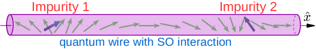
Figure 1: Schematic representation of the system composed of two magnetic impurities coupled to a quantum wire with spin-orbit interaction. Blue arrows represent the magnetic moments of the impurities while green arrows represent the spins of the conduction electrons that precess due to the spin-orbit coupling.

In a seminal paper published in 1990, Datta and Das proposed the idea of producing a highly spin-polarized current controlled via SOC by external electric field [20]. In their device, the spins of the electrons injected from a polarized source could be rotated by a tunable SOC while traveling towards a polarized drain. Likewise, it would interesting if one could use the SOC to control the indirect exchange interaction between two magnetic impurities embedded in a 1D conduction electron sea. The few studies addressing the RKKY interaction in one-dimensional systems with SOC, in general, employ a real space Green’s function [6]. It is known, however, that calculating the RKKY interaction in one-dimension is quite subtle [21]. This was first noticed by Kittel [22] and latter discussed in detail by Yafet [23]. Yafet indeed showed that, depending on how the double integral is handled, it can lead to unphysical results. Moreover, Yafet observed that the problem arises because the Pauli’s exclusion principle is severely violated. More recently, Rusin and Zawadzki [25] has examined the commonly used expression for the RKKY interaction [6] and noticed that there is an implicit change of order in a double-integration that requires extra care when used in one dimensional cases. Motivated by the interest in the physics of the RKKY interaction renewed in SOC materials, we revisit the calculation of the full indirect exchange interaction between two magnetic impurities in a 1D system. Based on the traditional second order perturbation theory, we obtain the known form of the inter-impurity couplings, which includes the usual RKKY, DM and Ising interaction terms. The effective couplings are calculated both numerically and analytically. Drastically different from the usual RKKY systems, we obtain additional oscillatory contributions to the effective couplings that do not decay with the distance. These unsuppressed terms vanish in the absence of SOC, in which case the traditional RKKY coupling is recovered. This feature is potentially important to spintronics as it can be used to control spin-spin interaction at longer distances as compared to the traditional RKKY couplings. Indeed, by employing a similar calculation we perform here, it was shown important enhancement in the magnetic coupling between magnetic impurity in controlled Rashba spin-orbit interaction[24]. There are currently several modern 1D systems with SOC that are natural candidates for experimental investigation of this interesting physics [27, 26, 28, 29, 30].

2 Model and method

We consider two spin-$1/2$ magnetic impurities[31] coupled to a quantum wire with spin-orbit interaction, as schematically shown in Fig. 1. We write the full Hamiltonian of the system as $H\!=\!H_{\mathrm{wire}}+H_{1}+H_{2}$, where

$$H_{\mathrm{wire}}=\sum_{k}\left(\varepsilon_{k}\delta_{ss^{\prime}}-\alpha_{\rm R}k\sigma^{y}_{ss^{\prime}}\right)c^{\dagger}_{ks}c_{ks^{\prime}}$$ (1)

describes the quantum wire, in which $c_{ks}^{\dagger}$ ($c_{ks}$) creates (annihilates) and electron with wave vector $k$, spin $s$ and energy $\varepsilon_{k}$. Here, $\varepsilon_{k}=\hbar^{2}k^{2}/2m^{*}$, where $m^{*}$ is the effective mass of the conduction electrons. The linear Rashba [32] spin-orbit coupling is described by the term proportional to $\alpha_{\rm R}$, with $\sigma^{\mu}$ representing the $\mu$-th the Pauli matrix. Finally, the couplings between the impurities and the conduction band are given by [33]

$$H_{i} = \frac{J}{N}\sum_{kk^{\prime}}e^{-i(k-k^{\prime})x_{i}}\left[S^{z}_{i}\left(c^{\dagger}_{k^{\prime}\uparrow}c_{k\uparrow}-c^{\dagger}_{k^{\prime}\downarrow}c_{k\downarrow}\right)+S^{+}_{i}c^{\dagger}_{k^{\prime}\downarrow}c_{k\uparrow}+S^{-}_{i}c^{+}_{k^{\prime}\uparrow}c_{k\downarrow}\right],$$ (2)

where $x_{i}$ (with $i=1,2$) is the position of the $i-$th impurity. We now derive an effective coupling between the two impurities mediated by the conduction electrons. Starting by diagonalizing the Hamiltonian (1), we follow the traditional second order perturbation theory approach. The resulting inter-impurity interaction is described by the effective Hamiltonian (see detail in A)

$$\tilde{H}_{{\rm imp}} = I_{\parallel}\tilde{S}_{1}^{z}\tilde{S}_{2}^{z}+\left(I_{\perp}\tilde{S}_{1}^{+}\tilde{S}_{2}^{-}+I_{\perp}^{*}\tilde{S}_{2}^{+}\tilde{S}_{1}^{-}\right).$$ (3)

The tildes on top of the spin operators above indicate that these operators are also written in the rotated basis. In Eq.(3) we have defined $I_{\parallel}\!=\!2{\rm Re\,}(I_{++}+I_{--})$ and $I_{\perp}\!=\!I_{-+}+I_{+-}^{*}$, where

$$I_{\delta\nu}=\frac{J^{2}}{4\pi^{2}}\!\int_{-k_{\delta}}^{k_{\delta}}dk\int_{|k^{\prime}|>k_{\delta}}dk^{\prime}\frac{e^{i(k-k^{\prime})x}{}}{\frac{\hbar^{2}}{2m^{*}}(k^{2}-k^{{}^{\prime}2})+\delta\alpha_{\rm R}(k-\delta\nu k^{\prime})}.$$ (4)

Here, $x=x_{2}-x_{1}$ is the distance between the impurities and $k_{\delta}=k_{\rm F}+\delta k_{\rm R}$, with $k_{\rm R}=m^{*}\alpha_{\rm R}/\hbar^{2}$ being the characteristic inverse of spin-orbit length. In the Eq.(4) we also have $\delta,\nu\in\{+,-\}$ denoting the Rashba bands. The rather simple form of the Hamiltonian (3), written in the Rashba basis, hides very interesting physics. It can be seen that $I_{\parallel}\neq I_{\perp}$, therefore, in the present form, the Hamiltonian (3) describes a highly anisotropic exchange interaction mediated by the conduction electrons. To highlight the physics buried in the Eq. (3) we transform it back to the original real spin basis, obtaining

$$\tilde{H}_{{\rm imp}} = I_{{\rm RKKY}}\mathbf{S}_{1}\cdot\mathbf{S}_{2}+I_{{\rm DM}}[(\mathbf{S}_{1}\times\mathbf{S}_{2})\cdot\hat{\bf y}]+I_{{\rm Ising}}S_{1}^{y}S_{2}^{y}.$$ (5)

Here, $I_{{\rm RKKY}}\!\!=2{\rm Re\,}I_{\perp}$, is the traditional RKKY interaction coupling renormalized by the SOC, $I_{{\rm DM}}\!\!\!=\!\!\!-2{\rm Im\,}I_{\perp}$ is the Dzaloshinkii-Moryia interaction between the two impurities and $I_{{\rm Ising}}\!\!=\!\!I_{\parallel}-2{\rm Re\,}I_{\perp}$ represents an Ising-like coupling. Again, for $\alpha_{\rm R}\!\!=\!\!0$ only the first term of (5) survives. In this case we left with one double integral, obtaining $I_{{\rm Ising}}\!=\!I_{\rm DM}\!=\!0$ and

$$I_{{\rm RKKY}}=4I_{0}\int_{-k_{\rm F}}^{k_{\rm F}}{dk}\int_{|k^{\prime}|>k_{\rm F}}{dk^{\prime}}\frac{\cos\left[(k-k^{\prime})x\right]}{k^{2}-k^{\prime 2}},$$ (6)

with $I_{0}={m^{*}J^{2}}/{2\pi^{2}\hbar^{2}}$. Performing the double integral (6) is known to be a delicate matter and have been discussed from way back [23]. Analytically, the integration can be performed if one extends the integral over $k^{\prime}$ to the entire real axis. After this, the residue theorem can be employed. Apart from the singular point $k^{\prime}\!\!=\!\!k\!\!=\!\!0$ (which can be accounted separately) the contribution to the double integral added by including the interval $(-k_{\rm F},k_{\rm F})$ vanishes because the integrand is antisymmetric under exchange $k^{\prime}\leftrightarrow k$. In the asymptotic limit $x\rightarrow\infty$, the final correct solution exhibits the usual form $\cos(2k_{\rm F}x)/x$.

In the presence of SOI $\alpha_{\rm R}\neq 0$, exact solutions for the integrals of Eq. (4) are, unfortunately, unavailable. In this case, even though we can subtract the contribution of the singularity from the integration over $k^{\prime}$ within the entire real axis, the integrand is no longer antisymmetric. Therefore, by extending the integral over $k^{\prime}$ to the interval $(-k_{\rm F},k_{\rm F})$, the extra contribution cannot be fully subtracted. As we will see below, great approximate solutions for the integrals (4) can still be obtained in the limit $k_{\rm R}\ll k_{\rm F}$, in which case the asymmetry of the integrand is negligible. To carry out the calculations, we simplify the notation defining $a=2k_{\rm R}$ and $\tilde{a}=a/k_{\rm F}$ and introducing the dimensionless momenta $q=k/k_{\rm F}$ and $q^{\prime}=k^{\prime}/k_{\rm F}$. Within these new variables, we can rewrite the Eq.(4) as

$$I_{\delta\nu}=I_{0}\int_{-q_{\delta}}^{q_{\delta}}{dq}\int_{|q^{\prime}|>q_{\delta}}\!\frac{e^{i(q-q^{\prime})k_{\rm F}x}dq^{\prime}}{(q^{2}-q^{\prime 2})+\delta\tilde{a}(q-\delta\nu q^{\prime})}.\\$$

Here, $q_{\delta}=1+\delta\tilde{a}/2=1+\delta k_{\rm R}/k_{\rm F}$. Following Yafet’s approach [23] we can write $I_{\delta\nu}=I_{\delta\nu}^{r}-I_{\delta\nu}^{\epsilon}$, where

$$I_{\delta\nu}^{r}=I_{0}\int_{-q_{\delta}}^{q_{\delta}}{dq}\int_{-\infty}^{\infty}\frac{e^{i(q-q^{\prime})k_{\rm F}x}dq^{\prime}}{(q^{2}-q^{\prime 2})+\delta\tilde{a}(q-\delta\nu q^{\prime})},$$ (7)

in which the integral over $q^{\prime}$ extends over the entire real axis, and $I_{\delta\nu}^{\epsilon}$ corresponds to the undesirable singularities accounted within the extended limit of the integral over $q^{\prime}$. The integration of (7) over $q^{\prime}$ can be performed using Cauchy’s integral theorem. For instance, after a cumbersome integration over $q$ (see detail in B) we obtain for $I_{\rm RKKY}$ (without the corrections),

$$I_{\rm{RKKY}}^{r} = \pi I_{0}\Big{\{}\sin(\tilde{a}k_{\rm F}x)\Big{[}{{\rm Ci}}\left[(1-\tilde{a})2k_{\rm F}x\right]-{{\rm Ci}}\left[(1+\tilde{a})2k_{\rm F}x\right]\Big{]}$$ (8)

$$+\cos(\tilde{a}k_{\rm F}x)\Big{[}{\rm Si}\left[(1+\tilde{a})2k_{\rm F}x\right]-{{\rm Si}}\left[(\tilde{a}-1)2k_{\rm F}x\right]$$

$$+{{\rm Si}}(2k_{\rm F}x)-{{\rm Si}}(-2k_{\rm F}x)\Big{]}-\ln\left|\frac{1-\tilde{a}}{1+\tilde{a}}\right|\sin(\tilde{a}k_{\rm F}x)\Big{\}}.$$

In the equation above, ${\rm Si}(x)$ and ${\rm Ci}(x)$ are the known sine and cosine integral functions, respectively [34]. To obtain the approximate expression we have to subtract the spurious contribution from the singularities. As an example, here we show in detail the calculation of the correction for $I_{-+}^{\epsilon}$ to the integral $I_{-+}$ (see B). Note that the unbalanced singularities occur when $q+q^{\prime}=0$ and $(q-q^{\prime}-\tilde{a})=0$ simultaneously, from which we find $q^{\prime}=-\tilde{a}/2=-q$. We can evaluate the integral within an infinitesimal interval around this point as

$$I^{\epsilon}_{-+}=I_{0}e^{i\tilde{a}k_{\rm F}x}\int_{\frac{\tilde{a}}{2}-\epsilon}^{\frac{\tilde{a}}{2}+\epsilon}dq\int_{\frac{-\tilde{a}}{2}-\epsilon}^{-\frac{\tilde{a}}{2}+\epsilon}\frac{dq^{\prime}}{(q+q^{\prime})(q-q^{\prime}-\tilde{a})},$$

with $\epsilon\rightarrow 0$. On the rhs of the Eq. (2) we have already used that at the singular point under analysis, $e^{i(q-q^{\prime})k_{\rm F}x}=e^{i(\tilde{a}+\tilde{a})k_{\rm F}x/2}=e^{i\tilde{a}k_{\rm F}x}$. Performing the integral over $q^{\prime}$ we obtain

$$I^{\epsilon}_{-+}=I_{0}e^{i\tilde{a}k_{\rm F}x}\!\int_{\frac{\tilde{a}}{2}-\epsilon}^{\frac{\tilde{a}}{2}+\epsilon}\!\!dq\frac{\ln|q-\frac{\tilde{a}}{2}+\epsilon|-\ln|q-\frac{\tilde{a}}{2}-\epsilon|}{q-\frac{\tilde{a}}{2}}.$$

After a simple change of variable $y=q-\tilde{a}/2$ we can write $I_{-+}^{\epsilon}=I_{0}e^{i\tilde{a}k_{\rm F}x}\int_{-\epsilon}^{\epsilon}dy\left[\frac{\ln|y+\epsilon|}{y}-\frac{\ln|y-\epsilon|}{y}\right].$ The integral here can be written in terms of the Dilogarithm function ${\rm Li}_{2}(x)=-\int_{0}^{x}dt\ln|1-t|/t$. With this and using $\rm{Li}_{2}(1)=\pi^{2}/6=-\rm{Li}_{2}(-1)$ [35] we can write $I_{-+}^{\epsilon}\!\!=\!\!({\pi^{2}}/{2})I_{0}e^{i\tilde{a}k_{\rm F}x}$. Proceeding likewise, we obtain the correction $I_{+-}^{\epsilon}=({\pi^{2}}/{2})I_{0}e^{-i\tilde{a}k_{\rm F}x}$. Collecting all these terms, the correction for the RKKY coupling is given by $I^{\epsilon}_{\rm{RKKY}}=2{\rm Re\,}(I_{-+}^{\epsilon}+I_{+-}^{\epsilon*})=4\pi I_{0}\left[\frac{\pi}{2}\cos(\tilde{a}k_{\rm F}x)\right].$ This is the quantity we must subtract from (8) to obtain the approximated result. This result generalizes the correction found in Ref. [25]. In the absence of SOC ($\tilde{a}=0$) $I^{\epsilon}_{\rm{RKKY}}\!=\!2\pi^{2}I_{0}$, which is exactly the correction discussed in Ref. [25]. The final expression for the RKKY coupling is then $I_{\rm RKKY}=I_{{\rm RKKY}}^{r}-I_{\rm RKKY}^{\epsilon}$.

Carrying out similar calculations we obtain the analytical results for all inter-impurity couplings,

$$I_{{\rm RKKY}} = \pi I_{0}\Big{\{}\sin(\tilde{a}k_{\rm F}x)\Big{[}{\rm Ci}\left[\left(1-\tilde{a}\right)2k_{F}x\right]-{\rm Ci}\left[\left(1+\tilde{a}\right)2k_{\rm F}x\right]\Big{]}$$ (11)

$$+\cos(\tilde{a}k_{\rm F}x)\Big{[}{\rm Si}\left[\left(1+\tilde{a}\right)2k_{\rm F}x\right]-\rm{{\rm Si}}\left[\left(\tilde{a}-1\right)2k_{\rm F}x\right]$$

$$+2{\rm Si}(2k_{\rm F}x)\Big{]}-{\ln}\left|\frac{1-\tilde{a}}{1+\tilde{a}}\right|\sin(\tilde{a}k_{\rm F}x)\Big{\}}-4\pi I_{0}\left[\frac{\pi}{2}\cos(\tilde{a}k_{\rm F}x)\right],$$

$$I_{{\rm DM}} = -\pi I_{0}\Big{\{}\cos(\tilde{a}k_{\rm F}x)\Big{[}{\rm Ci}\left[\left(1+\tilde{a}\right)2k_{F}x\right]-{\rm Ci}\left[\left(1-\tilde{a}\right)2k_{\rm F}x\right]\Big{]}$$ (12)

$$+\sin(\tilde{a}k_{\rm F}x)\Big{[}{\rm Si}\left[\left(1+\tilde{a}\right)2k_{\rm F}x\right]-\rm{{\rm Si}}\left[\left(\tilde{a}-1\right)2k_{F}x\right]$$

$$+2{\rm Si}(2k_{\rm F}x)\Big{]}+{\ln}\left|\frac{1-\tilde{a}}{1+\tilde{a}}\right|\cos(\tilde{a}k_{\rm F}x)\Big{\}}+4\pi I_{0}\left[\frac{\pi}{2}\sin\left(\tilde{a}k_{\rm F}x\right)\right],$$

$$I_{{\rm Ising}} = 2\pi I_{0}\Big{[}{\rm Si}\left[\left(1+\tilde{a}\right)2k_{\rm F}x\right]-{\rm Si}\left[\left(\tilde{a}-1\right)2k_{\rm F}x\right]\Big{]}-4\pi I_{0}\left(\frac{\pi}{2}\right)-I_{{\rm RKKY}}.$$ (13)

These rather complex expressions reduce to the known result $I_{{\rm RKKY}}=4\pi I_{0}[{{\rm Si}}(2k_{\rm F}x)-\pi/2]$ in the absence of SOC ($\tilde{a}=0$), that behaves as $\cos(2k_{\rm F}x)/x$ for large $x$ (with $I_{\rm DM}=I_{\rm Ising}=0$). On the other hand, for $\tilde{a}\neq 0$ the leading terms for large $x$ are

$$I_{{\rm RKKY}} = -\pi I_{0}{\ln}\left|\frac{k_{\rm F}-2k_{\rm R}}{k_{\rm F}+2k_{\rm R}}\right|\sin(2k_{\rm R}x),$$ (14)

$$I_{{\rm DM}} = -\pi I_{0}{\ln}\left|\frac{k_{\rm F}-2k_{\rm R}}{k_{\rm F}+2k_{\rm R}}\right|\cos(2k_{\rm R}x),$$ (15)

$$I_{{\rm Ising}} = \,\,\,\ \!\pi I_{0}{\ln}\left|\frac{k_{\rm F}-2k_{\rm R}}{k_{\rm F}+2k_{\rm R}}\right|\sin(2k_{\rm R}x).$$ (16)

Here we have used $\tilde{a}\!=\!2k_{\rm R}/k_{\rm F}$. These remarkable unsuppressed oscillatory terms summarize the main result of our work. These terms contrast with the decaying behavior of the usual RKKY interaction in the absence of SOC.

Before discussing these results, we compare the analytical results of Eqs. (11)-(13) with the ones obtained by direct numerical integration of (2) for $\tilde{a}=0.1$ ($k_{\rm R}=0.05k_{\rm F}$). The results are shown in Fig. 2. Panels 2(a), 2(b) and 2(c) correspond to the $I_{\rm RKKY}$, $I_{\rm DM}$ and $I_{\rm Ising}$, respectively. Dashed red lines correspond to the analytical results of Eqs. (11)-(13) while solid black lines refer to the numerical results obtained by direct integration of Eq. (2). The dash-dot blue lines show the asymptotic behavior of the coupling given by the Eqs. (14)-(16). The extraordinary agreement between our numerical and analytical results shown in Fig. 2 confirms that we have indeed obtained very good approximate expressions for all couplings.

The striking features are the undamped slow oscillations in the coupling due to the SOC mentioned earlier. The fast oscillations along the slow oscillating line is the traditional behavior of the RKKY interaction and result from the polarization of the Fermi sea by one impurity and “felt” by the other one. They are described by the ${\rm Ci}$ and ${{\rm Si}}$ functions of Eqs. (11)-(13) and have the traditional period $2\pi/2k_{\rm F}$. Note also in Eqs. (11)-(13) the extra terms $\pm 2\tilde{a}k_{\rm F}x=\pm 2k_{\rm R}x$ in the arguments of the functions ${{\rm Ci}}$ and ${\rm{\rm Si}}$. They are responsible for the curious beating patterns observed in the fast oscillations. Physically, the beating patterns can be understood in the following way: the original RKKY interaction exhibits an oscillation with frequency of $2k_{F}$. In the absence of SOC, the spin up and down bands are degenerated leading to a single Fermi momenta $k_{F}$. Here, on the other hand, electrons move freely in different helical bands possessing Fermi momenta are slightly shifted as compared to each other. Since the real spin basis representation is a linear combination of each Rashba bands, the resulting spin polarization is a combination of two oscillating terms whose phase are slightly shifted. This renders the beating pattern observed along the distance between the impurities. These beating patterns are akin to what was found in [36] for the RKKY interaction in spin-polarized bands.

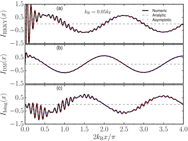
Figure 2: RKKY (a) Dzaloshinkii-Moryia (b) and Ising (c) couplings as a function of the distance $x$ between the impurities. Solid black lines correspond to the results obtained by direct numerical integration of Eq. (4), dashed red lines correspond to the analytical results of Eqs. (11)-(13) and dash-dot blue lines show the asymptotic behavior of the coupling given by the Eqs. (14)-(16).

3 Discussions

The unsuppressed oscillations obtained here can be understood as follows: after a given electron is scattered by the first impurity it travels throughout the quantum wire while its spin precesses due to the SOC. Since the momentum and spin are coupled together, this precession continues coherent until it collides with the second impurity. Somehow, the momentum-spin lock produced by the SOC in this 1D system provides a natural protection (not topological) that prevents the suppression of the couplings. To provide a better physical intuition, let us analyze the scattering processes involved in the second order perturbation theory. If we write the Hamiltonian (17) onto the Rashba basis we obtain

$$H_{i} = \frac{J}{N}\sum_{kk^{\prime}}e^{-i(k-k^{\prime})x_{i}}\left[\tilde{S}^{z}_{i}\left(c^{\dagger}_{k^{\prime}+}c_{k-}-c^{\dagger}_{k^{\prime}-}c_{k\dagger}\right)+\tilde{S}^{+}_{i}c^{\dagger}_{k^{\prime}\-}c_{k+}+\tilde{S}^{-}_{i}c^{+}_{k^{\prime}+}c_{k-}\right].$$ (17)

Here, again, the tilde on the spin operators emphasizes that they are also written on the Rashba basis, meaning that the “spin” scattering processes correspond to removing electrons from one band to another. Although the processes formally very much similar to those ones that occur in the absence of the SOC. Here, by virtue of the shift property $\varepsilon_{+}(k)=\varepsilon_{-}(k+Q)$ (where $Q=2k_{\rm R}$), the spin-flip processes in the second order perturbation theory involve intermediate states whose momenta is separated from the initial states by $2k_{\rm R}$ (for forward scattering process) or $2k_{\rm F}$ (for backscattering processes). In this sense, at zero temperature, conserving momenta scatterings are prevented by the SOC, which inhibits the decay of the couplings in the system. This analysis also allows us to understand enhancement of the oscillation amplitudes of Eqs. (14)-(16). When $k_{\rm F}\longrightarrow 2k_{\rm R}$ the Fermi momenta matches precisely the distance (in the momentum space) between the two bands, providing a resonant forward scattering. In reality, similarly to all the traditional approach to RKKY interaction, our results are limited distances smaller than the coherent length of the material. For distances larger than this characteristic length, other scattering processes have to be taken into account in the conduction electron propagation.

Somewhat similar to our results was found by J. Simonin [37]. He has found a spin-spin correlation between two magnetic moments induced by spin that extends also to distances longer than those of the traditional RKKY interaction. Our results also resemble the persistent spin helix [38, 39] in which a “right” combination of Rahsba and Dresselhaus SOCs produces a long lived spin excitation in the system. This contrasts with the traditional scattering in the absence of the SOC, in which there is a $Q=0$ scattering processes is allowed since the $\varepsilon_{\uparrow}(k)=\varepsilon_{\downarrow}(k)$. Previous studies usually employ a very attractive expression based on real space Green’s functions [6]. However, as thoroughly discussed by Valizadeh [36] the expression should be avoided in 1D systems. Essentially, the reason is because in the derivation of the equation (5) of Ref. [6] there is a change in the order of integration in double integral that should not be made in one-dimension. Here we circumvent this problem by directly performing the integrals (2) both analytically and numerically. See detailed discussion in D.

To interpret our results, let us recall that the mechanism responsible for the decaying oscillations in the RKKY interaction results from the existence of a Fermi sea. Under the second order perturbation theory perspective, the propagating electrons with momentum $k_{F}$ suffer scatterings with the Fermi sea. In the absence of SOC, these scatterings occur independently of the spin orientation of the propagating electrons. In contrast, in the presence of SOC, spin and momentum are locked together. As a result, an scattering can only occur if the spin orientation is modified accordingly. In 1D, backward scattering, for instance, has to be accompanied by a spin flip. Therefore, some of scatterings allowed in the absence of SOC are prevented when spin and momentum are coupled together.

4 Conclusions

We have investigated the exchange interaction between two magnetic impurities mediated by conduction electrons in a one-dimensional system with SOC. We revisited the calculation for the RKKY interaction in one-dimensional system by employing a straightforward second order perturbation theory of a two-impurities Kondo model. We find that in the presence of the SOC, the known RKKY, Dzaloshinkii-Moryia and Ising exchange interactions exhibit an additional oscillation resulting from the spin precession of the conduction electrons that mediate the exchange interactions. More interestingly, these additional oscillations do not decay with distance between the impurities. This is in sharp contrast to the results in the absence of the SOC that shows an RKKY coupling the behaves as $x^{-1}$. Moreover, our results also contrast with the recent calculations of RKKY interaction in 1D system with spin orbit [6]. The apparent difference between our results and the those from [6] arises from the fact that the expression used in the later cannot be straightforwardly applied in the 1D systems [36], specially in the presence of SOC Here, we avoid the problem by performing explicitly the integral resulting from the second order perturbations theory. Our work extends the expression for the 1D indirect exchange interactions to the case in which SOC is present. This is not only important because it is fundamentally distinct from the usual case in the absence of the SOC but also may be useful for practical application where long-distance couplings are relevant. Magnetic impurities in materials such as GaAs/AlGaAs [26] or InAs [27] spin-orbit coupled quantum wires are examples of potential candidates for experimental verification of our predictions.

Appendix

Appendix A Effective inter-impurities Hamiltonian

To derive the effective inter-impurities Hamiltonian we follow the traditional approach use to obtain the usual RKKY. We assume

$$H_{\mathrm{wire}}=\sum_{k}\left(\varepsilon_{k}\delta_{ss^{\prime}}-\alpha_{R}k\sigma^{y}_{ss^{\prime}}\right)c^{\dagger}_{ks}c_{ks^{\prime}},$$ (18)

as the unperturbed Hamiltonian that includes the spin-orbit interaction. The perturbation

$$H_{i} = \frac{J}{N}\sum_{kk^{\prime}}e^{-i(k-k^{\prime})x_{i}}\left[S^{z}_{i}\left(c^{\dagger}_{k^{\prime}\uparrow}c_{k\uparrow}-c^{\dagger}_{k^{\prime}\downarrow}c_{k\downarrow}\right)+S^{+}_{i}c^{\dagger}_{k^{\prime}\downarrow}c_{k\uparrow}+S^{-}_{i}c^{+}_{k^{\prime}\uparrow}c_{k\downarrow}\right]$$ (19)

accounts for the impurities. To apply the second order perturbation theory we diagonalize the Hamiltonian (18). This is achieved by defining the new operators by the transformation

$$\left(\begin{array}[]{c}c_{k+}\\ c_{k-}\end{array}\right)=\mathcal{U}_{k}\left(\begin{array}[]{c}c_{k\uparrow}\\ c_{k\downarrow}\end{array}\right),$$ (20)

where

$$\mathcal{U}_{k}=\frac{1}{\sqrt{2}}\left(\begin{array}[]{cc}1&1\\ -i&i\end{array}\right),$$ (21)

is a unitary matrix. The transformation above corresponds to a momentum-dependent rotation in the spin space. In the new base $H_{\mathrm{wire}}$ acquires the diagonal form

$$\tilde{H}_{\mathrm{wire}}=\sum_{kh}\varepsilon_{kh}c^{\dagger}_{kh}c_{kh},$$ (22)

in which $h=+,-$ is the helical quantum number and $\varepsilon_{kh}=\hbar k^{2}/2m^{*}+h\alpha_{R}k$ are the eigenvalues of $H_{\mathrm{wire}}$. The eigenstates are then defined as $|k,h\rangle$ such that $H_{\mathrm{wire}}|k,h\rangle=\varepsilon_{kh}|k,h\rangle$.

For simplicity, here we assume impurities have spin $1/2$ so that the spin operators can be easily written in terms of fermion operators as $S^{z}=(d^{\dagger}_{\uparrow}d_{\uparrow}-d^{\dagger}_{\downarrow}d_{\downarrow})/2$, $S^{+}=d_{\uparrow}^{{\dagger}}d_{\downarrow}$, and $S^{-}=d_{\downarrow}^{{\dagger}}d_{\uparrow}$, where $d^{\dagger}_{s}$ ($d_{s}$) corresponds to the creation (annihilation) spin-1/2 fermion operator. This is very useful because we can now perform the same rotation (20) for these fermion operators, after which we can rewrite (19) as

$$H_{i} = \frac{J}{N}\sum_{kk^{\prime}}e^{-i(k-k^{\prime})x_{i}}\left[\tilde{S}_{i}^{z}\left(c^{\dagger}_{k^{\prime}+}c_{k+}-c^{\dagger}_{k^{\prime}-}c_{k-}\right)+\tilde{S}_{i}^{+}c^{\dagger}_{k^{\prime}-}c_{k+}+\tilde{S}_{i}^{-}c^{+}_{k^{\prime}+}c_{k-}\right].$$ (23)

Here, the $\tilde{S}_{i}^{z}$ emphasizes that the impurity spin operators are written on the rotated spin basis. Having the eigenstates and eigenergies of the unperturbed Hamiltonian, the prescription to obtain the RKKY coupling is to compute the correction to the total energies up to the second order perturbation theory. To account for the degrees of freedom of the impurities, an eigenstate of $H_{\mathrm{wire}}$ can be written as $|k,h\rangle$, where $h$ is the helical quantum number.

The textbook expression for the second order energy correction can be written as

$$H_{\rm eff}=\sum_{k,h}^{\rm occ.}\,\sum_{{k^{\prime},h^{\prime}}}^{\rm empty}\frac{\langle k,h|(H_{1}+H_{2})|k^{\prime},h^{\prime}\rangle\langle k^{\prime},h^{\prime}|(H_{1}+H_{2})|k,h\rangle}{\varepsilon_{kh}-\varepsilon_{k^{\prime}h^{\prime}}},$$ (24)

where $H_{i}$ is given by (23). In the Eq. (24) we assume that we are at temperature $T=0$, in which case, the bands are fully occupied up to the Fermi level while fully empty above it. The exchange energy is only due the mixed terms of (24), we thus drop the self-interaction terms and write

$$\!\!\!\!\!\!\!\!\!\!\!\!\!\!H_{\rm eff} = \sum_{k,h}^{\rm occ.}\,\sum_{{k^{\prime},h^{\prime}}}^{\rm empty}\left[\frac{\langle k,h|H_{1}|k^{\prime},h^{\prime}\rangle\langle k^{\prime},h^{\prime}|H_{2}|k,h\rangle}{\varepsilon_{kh}-\varepsilon_{k^{\prime}h^{\prime}}}+\frac{\langle k,h|H_{2}|k^{\prime},h^{\prime}\rangle\langle k^{\prime},h^{\prime}|H_{1}|k,h\rangle}{\varepsilon_{kh}-\varepsilon_{k^{\prime}h^{\prime}}}\right].$$ (25)

The non-vanish contributions of (25) can be calculated applying the creator and annihilator operators on the state $|kh\rangle$. For example $\tilde{S}^{z}c_{k^{\prime}+}^{{\dagger}}c_{k+}|k,+\rangle=\tilde{S}^{z}|k^{\prime},+\rangle$, $\tilde{S}^{+}c_{k^{\prime}-}^{{\dagger}}c_{k+}|k,+\rangle=\tilde{S}^{+}|k^{\prime},-\rangle$, $\tilde{S}^{-}c_{k^{\prime}+}^{{\dagger}}c_{k-}|k,-\rangle=\tilde{S}^{-}|k^{\prime},+\rangle$. Using these relations we obtain

$$\langle k,+|H_{1}|k^{\prime},+\rangle = \frac{J}{N}\sum_{kk^{\prime}}e^{i(k-k^{\prime})x_{1}}\tilde{S}_{1}^{z};$$ (26)

$$\langle k,-|H_{1}|k^{\prime},-\rangle = -\frac{J}{N}\sum_{kk^{\prime}}e^{i(k-k^{\prime})x_{1}}\tilde{S}_{1}^{z},$$ (27)

$$\langle k,-|H_{1}|k^{\prime},+\rangle = \frac{J}{N}\sum_{kk^{\prime}}e^{i(k-k^{\prime})x_{1}}\tilde{S}_{1}^{+};$$ (28)

$$\langle k+|H_{1}|k^{\prime},-\rangle = \frac{J}{N}\sum_{kk^{\prime}}e^{i(k-k^{\prime})x_{1}}\tilde{S}_{1}^{-}.$$ (29)

Here we have used the orthogonality relation $\langle k,h|k^{\prime},h^{\prime}\rangle=\delta_{kk^{\prime}}\delta_{hh^{\prime}}$. Carrying out the calculation for $\langle k,h|H_{2}|k^{\prime},h^{\prime}\rangle$ we obtain similar results. Unlike the usual case of absence of SOC, in which the energy is equal for both spin components, here the energies $\varepsilon_{kh}$ depend of the helical number. Using $\varepsilon_{kh}=\hbar k^{2}/2m^{*}+h\alpha_{R}k$, the energy differences that appears in the denominator of the four non-vanishing terms of (25) are

$$\varepsilon_{k+}-\varepsilon_{k^{\prime}+} = \frac{\hbar^{2}}{2m^{*}}(k^{2}-k^{\prime 2})+\alpha_{R}(k-k^{\prime});$$ (30)

$$\varepsilon_{k-}-\varepsilon_{k^{\prime}-} = \frac{\hbar^{2}}{2m^{*}}(k^{2}-k^{\prime 2})-\alpha_{R}(k-k^{\prime}),$$ (31)

$$\varepsilon_{k-}-\varepsilon_{k^{\prime}+} = \frac{\hbar^{2}}{2m^{*}}(k^{2}-k^{\prime 2})-\alpha_{R}(k+k^{\prime});$$ (32)

$$\varepsilon_{k+}-\varepsilon_{k^{\prime}-} = \frac{\hbar^{2}}{2m^{*}}(k^{2}-k^{\prime 2})+\alpha_{R}(k+k^{\prime}).$$ (33)

Replacing the results of the Eqs. (26-A.12) and Eqs. (30-A.16) into Eq. (25) we obtain

$$H_{\rm imp} = (I_{++}+I_{++}^{*}+I_{--}+I_{--}^{*})\tilde{S}^{z}_{1}\tilde{S}^{z}_{2}+(I_{-+}+I^{*}_{+-})\tilde{S}^{+}_{1}\tilde{S}^{-}_{2}+(I_{+-}+I^{*}_{-+})\tilde{S}^{-}_{1}\tilde{S}^{+}_{2},$$

with

$$I_{\delta\nu}\!=\!\frac{J^{2}}{N^{2}}\sum_{k}^{\rm occupied}\,\sum_{k^{\prime}}^{\rm empty}\frac{e^{i(k-k^{\prime})x}}{\frac{\hbar^{2}}{2m^{*}}(k^{2}-k^{{}^{\prime}2})+\delta\alpha_{\rm R}(k-\delta\nu k^{\prime})},$$ (35)

in which $x=x_{2}-x_{1}$ is the distance between the impurities. The effective Hamiltonian (A) can be written in a more compact form

$$\tilde{H}_{\rm{imp}} = I_{\parallel}\tilde{S}^{z}_{1}\tilde{S}^{z}_{2}+I_{\perp}\tilde{S}^{+}_{1}\tilde{S}^{-}_{2}+I_{\perp}^{*}\tilde{S}^{-}_{2}\tilde{S}^{+}_{1},$$ (36)

where we have defined $I_{\parallel}=2{\rm Re\,}(I_{++}+I_{--})$ e $I_{\perp}=(I_{-+}+I_{+-}^{*})$. We now transform the summations into integrals using the usual prescription $(1/N)\sum_{k}\rightarrow(1/2\pi\int dk)$ in the limit $N\rightarrow\infty$, so that the Eq. (35) can now be written as

$$I_{\delta\nu}={J^{2}}\int_{-k_{\delta}}^{k_{\delta}}\frac{dk}{2\pi}\int_{|k^{\prime}|>k_{\delta}}\frac{dk^{\prime}}{2\pi}\frac{e^{i(k-k^{\prime})x}{}}{\frac{\hbar^{2}}{2m^{*}}(k^{2}-k^{{}^{\prime}2})+\delta\alpha_{\rm R}(k-\delta\nu k^{\prime})},$$ (37)

Here we also used the fact that, because of the SOC, the bands $+$ and $-$ have different Fermi momenta, namely $k_{\delta}=k_{F}+\delta k_{\rm R}$ (for $\delta=+,-$). In the helical basis, the Hamiltonian (36) has the form of a anisotropic Heisenberg Hamiltonian. Although simple, it hides the physics we want to study here. We can rewrite the impurity operators on the reals spin basis, on which we have

$$\tilde{S}^{+}_{1}\tilde{S}^{-}_{2} = \mathbf{S}_{1}\cdot\mathbf{S}_{2}+i(\mathbf{S}_{1}\times\mathbf{S}_{2})\cdot\hat{\bf y}-S^{y}_{1}S^{y}_{2},$$ (38)

$$\tilde{S}^{-}_{1}\tilde{S}^{+}_{2} = \mathbf{S}_{1}\cdot\mathbf{S}_{2}-i(\mathbf{S}_{1}\times\mathbf{S}_{2})\cdot\hat{\bf y}-S^{y}_{1}S^{y}_{2},$$ (39)

$$\tilde{S}^{z}_{1}\tilde{S}^{z}_{2} = S^{y}_{1}S^{y}_{2}.$$ (40)

Thus, in the real spin space, the exchange Hamiltonian is given by

$$\tilde{H}_{\rm{imp}}=I_{\rm{RKKY}}\mathbf{S}_{1}\cdot\mathbf{S}_{2}+I_{\rm{DM}}[(\mathbf{S}_{1}\times\mathbf{S}_{2})\cdot\hat{\bf y}]+I_{\rm{Ising}}S^{y}_{1}S^{y}_{2},$$ (41)

where, $I_{\rm{RKKY}}=2{\rm Re\,}[I_{\perp}]$, $I_{\rm{DM}}=-2{\rm Im\,}[I_{\perp}]$ and $I_{\rm{Ising}}=I_{\parallel}-2{\rm Re\,}[I_{\perp}]$ are the known RKKY, Dzaloshinkii-Moryia, and the Ising couplings.

Appendix B Analytical calculation of the couplings

We now focus on the calculation of the couplings $I_{\rm RKKY}$, $I_{\rm DM}$ and $I_{\rm Ising}$. This requires performing the integrals (37). To simplify the notation we define the dimensionless variables $q=k/k_{\rm F}$, $q^{\prime}=k^{\prime}/k_{\rm F}$, together with $a=2k_{\rm R}$, with $k_{\rm R}=m\alpha_{\rm R}/\hbar^{2}$, and $\tilde{a}=a/k_{\rm F}$. With these definitions the Eq. (37) acquires the form

$$I_{\delta\nu}=I_{0}\int_{-q_{\delta}}^{q_{\delta}}dq\int_{|q^{\prime}|>q_{\delta}}dq^{\prime}\frac{e^{i(q-q^{\prime})k_{F}x}}{(q^{2}-q^{{}^{\prime}2})+\delta\tilde{a}(q-\delta\nu q^{\prime})},$$ (42)

where $I_{0}=J^{2}m/2\pi^{2}\hbar^{2}$, and $q_{\delta}=1+\delta\tilde{a}/2$. An important point here that should be highlighted is that the order of the integrations above should not be changed as discussed by Yafet[23]. Later Valizedeh [36] revisited the problem and noted that the problem is that the integrals 37 do not obey the Fubini’s condition [40, 41], leading to different results depending on the order in which the integrations are performed. Here we keep the order of integrations as it is in Eq. (37), avoiding the aforementioned problem. To perform the integral over $q$ using the residues theorem we need to extend it to the entire real axis. With this we can write

$$I_{\delta\nu}^{r}=I_{0}\int_{-q_{\delta}}^{q_{\delta}}{dq}\int_{-\infty}^{\infty}dq^{\prime}\frac{e^{i(q-q^{\prime})k_{F}x}}{(q^{2}-q^{\prime 2})+\delta\tilde{a}(q-\delta\nu q^{\prime})}.$$ (43)

This deformation of the integral limits introduce undesirable contributions. If we are able to account for these extra contributions separately, we can subtract them from the final results to obtain the correct expression. In the absence of SOC, the integrand of (43) is antisymmetric under the exchange $q\longleftrightarrow q^{\prime}$, thus the extra contributions added to the results are solely those coming from corresponds to the singularities occurring at $q=q^{\prime}$. However, in the presence of the SOC ($\tilde{a}\neq 0$) the integrand is no longer antisymmetric. Therefore, there are contributions other than those arising from the singularities. Here we assume that the only relevant additional contributions are those arising from the singularities of 43. Thus, within this approximation, we can write $I_{\delta\nu}=I^{r}_{\delta\nu}-I^{\epsilon}_{\delta\nu}$, where and $I^{\epsilon}_{\delta\nu}$ corresponds to the undesirable singularities. We first integrate over $q^{\prime}$ and then over $q$. The Eq. (43) can be written as

$$I_{\delta\nu}^{r}=I_{0}\int_{-q_{\delta}}^{q_{\delta}}{dq}I_{\delta\nu}^{rq},$$ (44)

where we have defined

$$I_{\delta\nu}^{rq}=\mathcal{P}\oint dz\frac{e^{i(q-z)k_{F}x}}{(q^{2}-z^{2})+\delta\tilde{a}(q-\delta\nu z)}.$$ (45)

in the above $\mathcal{P}[\cdots]$ denote the Cauchy principal value.

Let us start with by calculating $I_{++}^{rq}$ that has the form

$$I^{rq}_{++}=\mathcal{P}\oint dz\frac{e^{i(q-z)k_{F}x}}{q^{2}-z^{2}+\tilde{a}(q-z)}.$$ (46)

Closing the contour on the lower half-plane and using the residues theorem we obtain

$$\mathcal{P}[I^{rq}_{++}]=\frac{2\pi}{2q+\tilde{a}}\sin[(q+\tilde{a}/2)k_{F}x]e^{i(q+\tilde{a}/2)k_{F}x}.$$ (47)

Noticing from (43) that we can obtain $I_{--}^{rq}$ by doing $\tilde{a}\rightarrow-\tilde{a}$ in the Eq. (47). Therefore we immediately obtain

$$\mathcal{P}[I^{rq}_{--}]=\frac{2\pi}{2q-\tilde{a}}\sin[(q-\tilde{a}/2)k_{F}x]e^{i(q-\tilde{a}/2)k_{F}x}.$$ (48)

Proceeding in a similar way for the other two integrals we obtain

$$\mathcal{P}[I^{rq}_{+-}]=\frac{2\pi}{2q+\tilde{a}}\sin[(q+\tilde{a}/2)k_{F}x]e^{i(q-\tilde{a}/2)k_{F}x}.$$ (49)

and

$$\mathcal{P}[I^{rq}_{-+}]=\frac{2\pi}{2q-\tilde{a}}\sin[(q-\tilde{a}/2)k_{F}x]e^{i(q+\tilde{a}/2)k_{F}x}.$$ (50)

Collecting the results (47)-(50) and grouping them properly, we obtain

$$I^{r}_{\rm{RKKY}} = 2{\rm Re\,}(I_{-+}^{r}+I_{+-*}^{r})$$

$$= 4\pi I_{0}\left[\int_{-q_{+}}^{q_{+}}dq\frac{\cos[(q-\tilde{a}/2)k_{F}x]\sin[(q+\tilde{a}/2)k_{F}x]}{2q+\tilde{a}}\right.$$

$$\left.+\int_{-q_{-}}^{q_{-}}dq\frac{\cos[(q+\tilde{a}/2)k_{F}x]\sin[(q-\tilde{a}/2)k_{F}x]}{2q-\tilde{a}}\right],$$

$$I^{r}_{\rm{DM}} = -2{\rm Im\,}(I_{-+}^{r}+I_{+-*}^{r})$$

$$= -4\pi I_{0}\left[\int_{-q_{-}}^{q_{-}}dq\frac{\sin[(q+\tilde{a}/2)k_{F}x]\sin[(q-\tilde{a}/2)k_{F}x]}{2q-\tilde{a}}\right.$$

$$\left.-\int_{-q_{+}}^{q_{+}}dq\frac{\sin[(q+\tilde{a}/2)k_{F}x]\sin[(q-\tilde{a}/2)k_{F}x]}{2q+\tilde{a}}\right],$$

and

$$I^{r}_{\rm{Ising}} = 2{\rm Re\,}(I_{++}^{r}+I_{--}^{r})-I^{r}_{\rm{RKKY}}$$

$$= 2\pi I_{0}\left[\int_{-q_{+}}^{q_{+}}dq\frac{\sin[(2q+\tilde{a})k_{F}x]}{2q+\tilde{a}}+\int_{-q_{-}}^{q_{-}}dq\frac{\sin[(2q-\tilde{a})k_{F}x]}{2q-\tilde{a}}\right]-I^{r}_{\rm{RKKY}}.$$

The superindices “$r$” denote the uncorrected results, i.e., before subtracting the extra contribution. The six integrals appearing in the expressions (B)-(B) above are rather complicated but can still be computed analytically. After a tiresome work, apart from additive constants, we obtain the expressions for the undefined integrals

$$\int dq\frac{\sin[(2q+\tilde{a})k_{F}x]}{2q+\tilde{a}} = \frac{1}{2}{\rm Si}[(2q+\tilde{a})k_{F}x],$$ (54)

$$\int dq\frac{\sin[(2q-\tilde{a})k_{F}x]}{2q-\tilde{a}} = \frac{1}{2}{\rm Si}[(2q-\tilde{a})k_{F}x],$$ (55)

$$\int dq\frac{\cos[(q-\tilde{a}/2)k_{F}x]\sin[(q+\tilde{a}/2)k_{F}x]}{2q+\tilde{a}} = \frac{1}{4}\Big{\{}-\sin(\tilde{a}k_{F}x){\rm Ci}[(2q+\tilde{a})k_{F}x].$$

$$+\cos(\tilde{a}k_{F}x){\rm Si}[(2q+\tilde{a})k_{F}x]$$

$$+\sin(\tilde{a}k_{F}x)\ln[2(2q+\tilde{a})]\Big{\}},$$

$$\int dq\frac{\cos[(q+\tilde{a}/2)k_{F}x]\sin[(q-\tilde{a}/2)k_{F}x]}{2q-\tilde{a}} = \frac{1}{4}\Big{\{}\sin(\tilde{a}k_{F}x){\rm Ci}[(2q-\tilde{a})k_{F}x]$$

$$-\cos(\tilde{a}k_{F}x){\rm Si}[(\tilde{a}-2q)k_{F}x]$$

$$-\sin(\tilde{a}k_{F}x)\ln[2(\tilde{a}-2q)]\Big{\}},$$

$$\int dq\frac{\sin[(q-\tilde{a}/2)k_{F}x]\sin[(q+\tilde{a}/2)k_{F}x]}{2q+\tilde{a}} = \frac{1}{4}\Big{\{}-\cos(\tilde{a}k_{F}x){\rm Ci}[(2q+\tilde{a})k_{F}x]$$

$$-\sin(\tilde{a}k_{F}x){\rm Si}[(2q+\tilde{a})k_{F}x]$$

$$+\cos(\tilde{a}k_{F}x){\ln}[2(2q+\tilde{a})]\Big{\}},$$

and

$$\int dq\frac{\sin[(q+\tilde{a}/2)k_{F}x]\sin[(q-\tilde{a}/2)k_{F}x]}{2q-\tilde{a}} = \frac{1}{4}\Big{\{}-\cos(\tilde{a}k_{F}x){\rm Ci}[(2q-\tilde{a})k_{F}x]$$

$$-\sin(\tilde{a}k_{F}x){\rm Si}[(\tilde{a}-2q)k_{F}x]$$

$$\quad+\cos(\tilde{a}k_{F}x)\ln[2(\tilde{a}-2q)]\Big{\}}.$$

In the above we use the usual definitions

$${\rm Ci}(x) = \int_{0}^{x}\frac{\cos(t)}{t}dt$$ (60)

$${\rm{\rm Si}}(x) = \int_{0}^{x}\frac{\sin(t)}{t}dt.$$ (61)

After imposing the proper limits to the results (54)-(B) and some algebraic manipulations we can write

$$I^{r}_{{\rm RKKY}} = \pi I_{0}\Big{\{}\sin(\tilde{a}k_{F}x)\Big{[}{\rm Ci}\left[(1-\tilde{a})2k_{F}x\right]-{\rm Ci}\left[(1+\tilde{a})2k_{F}x\right]\Big{]}$$ (62)

$$+\cos(\tilde{a}k_{F}x)\Big{[}{\rm Si}\left[(1+\tilde{a})2k_{F}x\right]-{\rm Si}\left[(\tilde{a}-1)2k_{F}x\right]$$

$$+2{\rm Si}(2k_{F}x)\Big{]}-{\ln}\left|\frac{1-\tilde{a}}{1+\tilde{a}}\right|\sin(\tilde{a}k_{F}x)\Big{\}},$$

$$I^{r}_{{\rm DM}} = -\pi I_{0}\Big{\{}\cos(\tilde{a}k_{F}x)\Big{[}{\rm Ci}\left[(1+\tilde{a})2k_{F}x\right]-{\rm Ci}\left[(1-\tilde{a})2k_{F}x\right]\Big{]}$$ (63)

$$+\sin(\tilde{a}k_{F}x)\Big{[}{\rm Si}\left[(1+\tilde{a})2k_{F}x\right]-{\rm Si}\left[(\tilde{a}-1)2k_{F}x\right]$$

$$+2{\rm Si}(2k_{F}x)\Big{]}+{\ln}\left|\frac{1-\tilde{a}}{1+\tilde{a}}\right|\cos(\tilde{a}k_{F}x)\Big{\}},$$

$$I^{r}_{{\rm Ising}} = 2\pi I_{0}\Big{[}{\rm Si}((1+\tilde{a})2k_{F}x)-{\rm Si}\left[(\tilde{a}-1)2k_{F}x\right]\Big{]}-I^{r}_{{\rm RKKY}}.$$ (64)

To obtain the final results we still need to compute the contribution from the singularities of the integrals (43).

B.1 Contribution from the singularities

To compute the contributions from the singularities we use the same method applied to the traditional RKKY problem in 1D [23, 25]. Let us start with the integral

$$I_{++}=I_{0}\int_{-q_{+}}^{q_{+}}dq\int_{|q^{\prime}|>q_{+}}dq^{\prime}\frac{e^{i(q-q^{\prime})k_{F}x}}{q^{2}-{q^{\prime}}^{2}+\tilde{a}(q-q^{\prime})}.$$

The singularities of this integral occur when $(q-q^{\prime})=0$ and $(q+q+\tilde{a})=0$ or $q^{\prime}=-\tilde{a}/2$ and $q=-\tilde{a}/2$. In the following we calculate the integral above around $q=q^{\prime}=\tilde{a}/2$. At this point we have $e^{i(q-q^{\prime})k_{F}x}=e^{i(-\tilde{a}+\tilde{a})k_{F}x/2}=1$. Therefore,

$$I_{++}^{\epsilon}=\int_{-\frac{\tilde{a}}{2}-\epsilon}^{-\frac{\tilde{a}}{2}+\epsilon}dq\int_{-\frac{\tilde{a}}{2}-\epsilon}^{-\frac{\tilde{a}}{2}+\epsilon}\frac{dq^{\prime}}{(q-q^{\prime})(q+q^{\prime}+\tilde{a})},$$ (66)

with $\epsilon\rightarrow 0^{+}$. The integral over $q^{\prime}$ variable can be calculated analytically using

$$\int\frac{dx}{(y-x)(y+x+a)} = \frac{\ln(-a-x-y)-\ln(y-x)}{2y+a}+\mbox{constant}.$$ (67)

Imposing the limits, after some algebraic manipulation we obtain

$$I_{++}^{\epsilon}\!\!=\!\!\int_{-\frac{\tilde{a}}{2}-\epsilon}^{-\frac{\tilde{a}}{2}+\epsilon}\!\!dq\frac{\ln|(q+\tilde{a}/2)+\epsilon|-\ln|(q+\tilde{a}/2)-\epsilon|}{q+\tilde{a}/2}.$$ (68)

Performing the variable change $x=q+\tilde{a}/2$ the above integral becomes

$$I_{++}^{\epsilon}=\int_{-\epsilon}^{\epsilon}dx\left[\frac{\ln|x+\epsilon|}{x}-\frac{\ln|x-\epsilon|}{x}\right].$$ (69)

This expression can be written as

$$I_{++}^{\epsilon} = \int_{-1}^{1}du\left[\frac{\ln|1+u|}{u}-\frac{\ln|1-u|}{x}\right]=2\rm{Li}_{2}(1)-2\rm{Li}_{2}(-1)=\frac{\pi^{2}}{2},$$ (70)

where

$$\rm{Li}_{2}(x)=-\int_{0}^{x}\frac{\ln|1-t|}{t}dt$$ (71)

is the Dilogarithmic function. In the last line passage in (70) we have used[35] $\rm{Li}_{2}(1)=\pi^{2}/6$ and $\rm{Li}_{2}(-1)=-\pi^{2}/12$.

Likewise, we can show that

$$I^{\epsilon}_{--}=\frac{\pi^{2}}{2}.$$ (72)

The others two integrals render slightly different results. Let us look at the correction for

$$I_{+-}=I_{0}\int_{-q_{+}}^{q_{+}}dq\int_{-\infty}^{\infty}dq^{\prime}\frac{e^{i(q-q^{\prime})k_{F}x}}{q^{2}-{q^{\prime}}^{2}+\tilde{a}(q+q^{\prime})}.$$ (73)

Here the contribution are accounted when $(q+q^{\prime})=0$ and $(q-q^{\prime}+\tilde{a})=0$, from which we extract $q^{\prime}=\tilde{a}/2$ and $q=-\tilde{a}/2$. At this point, $e^{i(q-q^{\prime})k_{F}x}=e^{i(-\tilde{a}-\tilde{a})k_{F}x/2}=e^{-i\tilde{a}k_{F}x}$, so that

$$I^{\epsilon}_{+-}=e^{-i\tilde{a}k_{F}x}\int_{-\frac{\tilde{a}}{2}-\epsilon}^{-\frac{\tilde{a}}{2}+\epsilon}dq\int_{\frac{\tilde{a}}{2}-\epsilon}^{\frac{\tilde{a}}{2}+\epsilon}\frac{dq^{\prime}}{(q+q^{\prime})(q-q^{\prime}+\tilde{a})}.$$

Using the indefinite integral

$$\int\!\!\!\frac{dx}{(y+x)(y-x+a)}\! = \!\frac{\ln(y+x)-\ln(-a+x-y)}{2y+a}+\mbox{constant},$$ (75)

we obtain

$$I^{\epsilon}_{+-} = e^{-i\tilde{a}k_{F}x}$$

$$\!\!\!\!\!\!\times\int_{-\frac{\tilde{a}}{2}-\epsilon}^{-\frac{\tilde{a}}{2}+\epsilon}\!\!\!\!\!dq\frac{\ln|(q+\tilde{a}/2)+\epsilon|\!-\!{\ln}|(q+\tilde{a}/2)-\epsilon|}{q+\tilde{a}/2}.$$

Apart from the prefactor $e^{-i\tilde{a}k_{F}x}$, this is the same as in 68, therefore,

$$I^{\epsilon}_{+-}=\frac{\pi^{2}}{2}e^{-i\tilde{a}k_{F}x}.$$ (77)

The last correction, for $I_{-+}^{r}$, can be obtained using same argument of changing $\tilde{a}\rightarrow-\tilde{a}$ in (77), leading to

$$I^{\epsilon}_{-+}=\frac{\pi^{2}}{2}e^{i\tilde{a}k_{F}x}.$$ (78)

Collecting the results of (70), (72), (77) and (78) we obtain the corrections for the couplings

$$I^{\epsilon}_{\rm{RKKY}} = 2{\rm Re\,}(I_{-+}^{\epsilon}+I_{+-}^{\epsilon*})=4\pi I_{0}\left[\frac{\pi}{2}\cos(\tilde{a}k_{F}x)\right],$$

$$I^{\epsilon}_{\rm{DM}} = -2{\rm Im\,}(I_{-+}^{\epsilon}+I_{+-}^{\epsilon*})=-4\pi I_{0}\left[\frac{\pi}{2}\sin(\tilde{a}k_{F}x)\right],$$

$$I^{\epsilon}_{\rm{Ising}} = 2{\rm Re\,}(I_{++}^{\epsilon}+I_{--}^{\epsilon})-I^{\epsilon}_{\rm{RKKY}}$$ (81)

$$= 4\pi I_{0}\left(\frac{\pi}{2}\right)-I^{\epsilon}_{\rm{RKKY}}.$$

We now subtract the results of the Eqs. (B.1) from those of Eqs. (62) to obtain our final analytical results for the indirect coupling

$$I_{{\rm RKKY}} = \pi I_{0}\Big{\{}\sin(\tilde{a}k_{F}x)\Big{[}{\rm Ci}\left[(1-\tilde{a})2k_{F}x\right]-{\rm Ci}\left[(1+\tilde{a})2k_{F}x\right]\Big{]}$$ (82)

$$+\cos(\tilde{a}k_{F}x)\Big{[}{\rm Si}\left[(1+\tilde{a})2k_{F}x\right]-{\rm Si}\left[(\tilde{a}-1)2k_{F}x\right]$$

$$+2{\rm Si}(2k_{F}x)\Big{]}-{\ln}\left|\frac{1-\tilde{a}}{1+\tilde{a}}\right|\sin(\tilde{a}k_{F}x)\Big{\}}-4\pi I_{0}\left[\frac{\pi}{2}\cos(\tilde{a}k_{F}x)\right],$$

$$I_{{\rm DM}} = -\pi I_{0}\Big{\{}\cos(\tilde{a}k_{F}x)\Big{[}{\rm Ci}\left[(1+\tilde{a})2k_{F}x\right]-{\rm Ci}\left[(1-\tilde{a})2k_{F}x\right]\Big{]}$$ (83)

$$+\sin(\tilde{a}k_{F}x)\Big{[}{\rm Si}\left[(1+\tilde{a})2k_{F}x\right]-{\rm Si}\left[(\tilde{a}-1)2k_{F}x\right]$$

$$+2{\rm Si}(2k_{F}x)\Big{]}+{\ln}\left|\frac{1-\tilde{a}}{1+\tilde{a}}\right|\cos(\tilde{a}k_{F}x)\Big{\}}+4\pi I_{0}\left[\frac{\pi}{2}\sin(\tilde{a}k_{F}x)\right],$$

$$I_{{\rm Ising}} = 2\pi I_{0}\Big{[}{\rm Si}\left[(1+\tilde{a})2k_{F}x\right]-{\rm Si}\left[(\tilde{a}-1)2k_{F}x\right]\Big{]}-4\pi I_{0}\left(\frac{\pi}{2}\right)-I_{{\rm RKKY}}.$$ (84)

Notice that if we take $\tilde{a}=0$ the usual result $I_{\rm{RKKY}}=4\pi I_{0}\left[{\rm Si}(2k_{F}x)-{\pi}/{2}\right]$ and $I_{\rm{DM}}=I_{\rm{Ising}}=0$ is recovered, as expected. Interestingly, however, the asymptotic behavior of these expressions are

$$I_{{\rm RKKY}} = -\pi I_{0}{\ln}\left|\frac{k_{\rm F}-2k_{\rm R}}{k_{\rm F}+2k_{\rm R}}\right|\sin(2k_{\rm R}x),$$ (85)

$$I_{{\rm DM}} = -\pi I_{0}{\ln}\left|\frac{k_{\rm F}-2k_{\rm R}}{k_{\rm F}+2k_{\rm R}}\right|\cos(2k_{\rm R}x),$$ (86)

$$I_{{\rm Ising}} = \,\,\,\ \!\pi I_{0}{\ln}\left|\frac{k_{\rm F}-2k_{\rm R}}{k_{\rm F}+2k_{\rm R}}\right|\sin(2k_{\rm R}x).$$ (87)

Where we use $\lim_{x\rightarrow\infty}{\rm Ci}(x)=0$, and $\lim_{x\rightarrow\infty}{\rm Si}(x)=\pi/2$. These unsuppressed oscillations appearing in these asymptotic expressions is the principal result of our work.

Appendix C Analytical vs. numerical results

Despite the complexities involved in obtaining the analytical results, numerically it is rather straightforward. Basically, we need to calculate the integrals (37) numerically. In fact, here we simply perform these integrals using a numerical subroutine built in Julia programming language[42]. To get convergence, as usual we add an infinitesimal imaginary to the denominator of (37) so that the integrals we indeed solve numerically are

Figure 3: Comparison between the analytical and the numerical results for the RKKY vs $x$ in the absence of SOC ($a=0$). Solid black lines correspond to the numerical results while dashed red lines correspond to the analytical results. The blue dashed line shows a function $\sim 1/x$ to show that in the absence of the SOC the RKKY coupling indeed decays as expected.

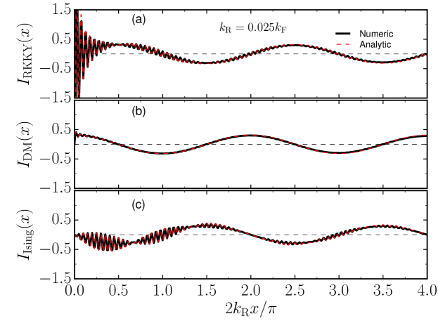
Figure 4: Comparison between the analytical and the numerical results for the indirect couplings. RKKY (a) Dzaloshinkii-Moryia (b) and Ising (c) couplings as a function of $x$ for $k_{R}=0.025k_{\rm F}$. Solid black lines correspond to the numerical results, dashed red lines correspond to the analytical results and dash-dot blue lines show the asymptotic behavior of the couplings.

$$I_{\delta\nu}={J^{2}}\int_{-k_{\delta}}^{k_{\delta}}\frac{dk}{2\pi}\int_{|k^{\prime}|>k_{\delta}}\frac{dk^{\prime}}{2\pi}\frac{e^{i(k-k^{\prime})x}}{\frac{\hbar^{2}}{2m^{*}}(k^{2}-k^{{}^{\prime}2})+\delta\alpha_{\rm R}(k-\delta\nu k^{\prime})+i\eta},$$ (88)

with $\eta=0^{+}$. The expression above is exactly the same we obtain when we used scattering theory to obtain the indirect interaction via the Lippmann-Schwinger equation [43], having in mind that we need to account for the Fermi sea and the Pauli’s exclusion principle. Having calculated the integrals numerically, we obtain the indirect coupling using the expressions just using the expressions for $I_{{\rm RKKY}}$, $I_{{\rm DM}}$ and $I_{\rm Ising}$ obtained in the end of Sec. (A). The analytical (dashed red line) and the numerical (solid black line) results are compared in Fig. (3) in the absence of SOC ($a=0$) and in Fig (4) for $k_{R}=0.025k_{\rm F}$. Notice that, as expected, the oscillations are suppressed as $1/x$, as shown by the dashed blue line.

Appendix D Effective Hamiltonian in terms of Green’s function

In this section we present a derivation of an expression for the effective Inter-impurity Hamiltonian in terms of Green’s function in the position space for the 1D system in the presence of the spin-orbit interaction.

Let us start with Eq. (25) that can be written as

$$\!H_{\rm eff}\!=\!\!\sum_{k,h}^{\rm occ.}\,\sum_{{k^{\prime},h^{\prime}}}^{\rm empty}\left[\frac{\langle k,h|H_{1}|k^{\prime},h^{\prime}\rangle\langle k^{\prime},h^{\prime}|H_{2}|k,h\rangle}{\varepsilon_{kh}-\varepsilon_{k^{\prime}h^{\prime}}}\!+\!{\rm H.c}\right].$$

Defining the retarded Green’s function

$$\hat{G}_{k^{\prime},h^{\prime}}(\varepsilon_{kh})=\frac{|k^{\prime},h^{\prime}\rangle\langle k^{\prime},h^{\prime}|}{\varepsilon_{kh}-\varepsilon_{k^{\prime}h^{\prime}}},$$ (90)

in which $\varepsilon_{kh}\rightarrow\varepsilon_{kh}+0^{+}$, the Eq. (D) can be written as

$$H_{\rm eff}=\sum_{k,h}^{\rm occ.}\,\sum_{{k^{\prime},h^{\prime}}}^{\rm empty}{\langle k,h|H_{1}\hat{G}_{k^{\prime},h^{\prime}}(\varepsilon_{kh})H_{2}|k,h\rangle}+{\rm H.c.}$$ (91)

Let us now introduce two closure relations in the position space, $\sum_{x,\sigma}|x,\sigma\rangle\langle x,\sigma|$, to obtain

$$\!\!\!\!\!\!\!\!\!\!\!\!\!\!\!\!\!H_{\rm eff} = \sum_{k,h}^{\rm occ.}\sum_{k^{\prime},h^{\prime}}^{\rm empty}\sum_{xx^{\prime}}\sum_{\sigma\sigma^{\prime}}\langle k,h|H_{1}|x,\sigma\rangle\langle x,\sigma|\hat{G}_{k^{\prime},h^{\prime}}(\varepsilon_{kh})|x^{\prime},\sigma^{\prime}\rangle\langle x^{\prime},\sigma^{\prime}|H_{2}|k,h\rangle+{\rm H.c.}.\quad$$ (92)

In the real position and spin space, the Hamiltonian $H_{i}$ of Eq. (23) acquires the form

$$H_{i} = J\left[S^{z}_{x}(c^{\dagger}_{x\uparrow}c_{x\uparrow}-c^{\dagger}_{x\downarrow}c_{x\downarrow})+S^{+}_{x}c^{\dagger}_{x\downarrow}c_{x\uparrow}\right.$$ (93)

$$\left.+S^{-}_{x}c^{\dagger}_{x\uparrow}c_{x\downarrow}\right]\delta(x-x_{i})=H(x)\delta(x-x_{i}).$$

Inserting this into Eq. (92), after some straightforward algebraic manipulations we obtain

$$H_{\rm eff} = J^{2}\sum_{hh^{\prime}}\langle h|\left({\bf S}_{1}\cdot{\bf s}\right)|h^{\prime}\rangle\langle h^{\prime}|\left({\bf S}_{2}\cdot{\bf s}\right)|h\rangle$$ (94)

$$\times\sum_{k}^{\rm occ.}\sum_{k^{\prime}}^{\rm empty}G_{k^{\prime},h^{\prime}}(x_{1},x_{2},\varepsilon_{kh})\langle k|x_{1}\rangle\langle x_{2}|k\rangle+{\rm H.c.}.$$

Here we have defined the scalar retarded Green’s function

$$G_{k^{\prime},h^{\prime}}(x_{1},x_{2},\varepsilon_{kh})=\frac{\langle x_{1}|k^{\prime}\rangle\langle k^{\prime}|x_{2}\rangle}{\varepsilon_{kh}-\varepsilon_{k^{\prime}h^{\prime}}}.$$ (95)

We now use $\langle x_{i}|k\rangle=\frac{1}{\sqrt{N}}e^{ikx_{i}}$ and transform the summation into integrals we obtain

$$H_{\rm eff} = NJ^{2}\sum_{hh^{\prime}}\langle h|\left({\bf S}_{1}\cdot{\bf s}\right)|h^{\prime}\rangle\langle h^{\prime}|\left({\bf S}_{2}\cdot{\bf s}\right)|h\rangle$$ (96)

$$\!\!\!\times\int_{\rm occ.}\frac{dk}{2\pi}e^{ik(x_{2}-x_{1})}\int_{\rm empty}\frac{dk^{\prime}}{2\pi}G_{k^{\prime},h^{\prime}}(x_{1},x_{2},\varepsilon_{kh})+{\rm H.c.}.$$

As discussed in detail by Valizadeh[36], further simplification of Eq. (96) towards the a similar expression as Eq. (5) of Ref. [6] requires changing the order of the integrals over $k$ and $k^{\prime}$, which may lead to spurious result in 1D case. Moreover, the integral over $k^{\prime}$ cannot be extended from $-\infty$ to $\infty$, since the extra contribution to the double integral does not vanish in the presence of spin-orbit coupling.

References

References

• [1] C. Kittel, Quantum Theory of Solids, John Wiley & Sons, Inc. (1987).
• [2] J. H. Van Vleck, Rev. of Mod. Phys. 34, 681 (1962).
• [3] A. Ruderman and C. Kittel, Phys. Rev. 96, 99 (1954).
• [4] T. Kasuya, Prog. Theor. Phys. 16, 45 (1956).
• [5] K. Yosida, Phys. Rev. 106, 893 (1957).
• [6] I. Imamura, P. Bruno and U. Yasuhiro, Phys. Rev. 69, 121303 (R) (2004)
• [7] Andreas Schulz, Alessandro De Martino, Philip Ingenhoven, and Reinhold Egger, Phys. Rev. B 79, 205432 (2009).
• [8] A. Kundu and S. Zhang, Phys. Rev. B 92, 094434 (2015).
• [9] Shi-Xiong Wang, Hao-Ran Chang and Jianhui Zhou, Phys. Rev. B 96, 115204 (2017).
• [10] D. Mastrogiuseppe, N. Sandler, and S. E. Ulloa, Phys. Rev. B 93, 094433 (2016).
• [11] Hao-Ran Chang, Jianhui Zhou, Shi-Xiong Wang, Wen-Yu Shan and Di Xiao, Phys. Rev. B 92, 241103(R) (2015).
• [12] Jia-Ji Zhu, Kai Chang, Ren-Bao Liu, and Hai-Qing Lin, Phys. Rev. B 81, 113302 (2010).
• [13] J. Klinovaja and D. Loss, Phys. Rev. B 87, 045422 (2013).
• [14] I. Dzyaloshinsky, J. Phys. Chem. Solids 4, 241 (1958).
• [15] T. Moriya, Phys. Rev. Lett. 4, 228 (1960); T. Moriya, Phys. Rev. 120, 91 (1960).
• [16] David F. Mross and Henrik Johannesson, Phsy. Rev. B, 80, 155302 (2009).
• [17] Semiconductor Spintronics, and Quantum Computation, Nanoscience and Technology, edited by D. D. Awshalom, D. Loss, and N. Samarth Springer-Verlag, Berlin, (2002).
• [18] Jifa Tian, Seokmin Hong, Ireneusz Miotkowski, Supriyo Datta, and Yong P. Chen, Science Advances 14, e1602531 (2017).
• [19] G. R. de Sousa, Joelson F. Silva, and E. Vernek, Phys. Rev. B 94, 125115 (2016).
• [20] S. Datta and B. Das, Appl. Phys. Lett. 56, 665 (1990).
• [21] Gabriele F. Giuliani, Giovanni Vignale, and Trinanjan Datta, Phys. Rev. B 72, 033411 (2005).
• [22] C. Kittel, in Solid State Physics, edited by F. Seitz, D. Turnbull, and H. Ehrenreich (Academic, New York, 1968), Vol. 22, p. 1.
• [23] Y. Yafet, Phys. Rev. B 36, 3948 (1987).
• [24] Pin Lyua and Ning-Ning Liu, Journal of Applied Physics 102, 103910 (2007).
• [25] T. M. Rusin and W. Zawadzki, Journal of Magnetism and Magnetic Materials 441, 387 (2017).
• [26] C. H. L. Quay, T. L. Hughes, J. A. Sulpizio, L. N. Pfeiffer, K.W. Baldwin, K.W.West, D. Goldhaber-Gordon and R. de Picciotto, Nature Phys. 6, 336 (2010).
• [27] Dong Liang and Xuan P.A. Gao, Nano Lett. 12, 3263 (2012).
• [28] Victor Galitski, Ian B. Spielman, Nature 494, 11841 (2013)
• [29] O. Klochan, A. P. Micolich, L. H. Ho, A. R. Hamilton, K. Muraki and Y. Hirayama, New Journal of Physics 11 043018 (2009).
• [30] Lawrence W. Cheuk, Ariel T. Sommer, Zoran Hadzibabic, Tarik Yefsah, Waseem S. Bakr, and Martin W. Zwierlein, Phys. Rev. Lett. 109, 095302 (2012).
• [31] Considering spin-$1/2$ impurities is not really necessary here, however, it makes our calculation simpler, as we can write straightforwardly write the spin operator of the impurity in terms of the Pauli matrices.
• [32] E. I. Rashba, Sov. Phys. Solid State 2, 1109 (1960).
• [33] W. Nolting and A. Ramakanth, Quantum Theory of Magnetism, Springer Heidelberg Dordrecht London New York (2009).
• [34] As usual, the sine and cossine integral functions are respectively defined as ${\rm Ci}(x)=\int_{0}^{x}(1/t){\cos(t)}dt$ and ${\rm{\rm Si}}(x)=\int_{0}^{x}(1/t){\sin(t)}dt$.
• [35] W. Grobner and N. Hofreiter, Integralrafel (Springer-Verlag, New York, 1957), Vol. 1.
• [36] M. M. Valizadeh, International Journal of Modern Physics B 30, 1650234 (2016).
• [37] J. Simonin, Phys. Rev. Lett. 97, 266804 (2006).
• [38] B. A. Bernevig, J. Orenstein, and Shou-Cheng Zhang, Phys. Rev. Lett. 97, 236601 (2006).
• [39] J. D. Koralek, C. P. Weber, J. Orenstein, B. A. Bernevig, Shou-Cheng Zhang, S. Mack and D. D. Awschalom, Nature 458, 610 (2009).
• [40] G. Fubini, Rom. Acc. L. Rend. 16, 608 (1907); Reprinted in G. Fubini, Opere Scelte 2, 243 (1958).
• [41] H. Friedman, Illinois J. Math. 24, 390395 (1980).
• [42] J. Bezanson, A. Edelman, S. Karpinski, and V. B. Shah, SIAM Rev., 59(1), 65–98 (2017).
• [43] J. J. Sakurai, Modern quantum mechanics, Addison-Wesley (1994).