Large-$N_{c}$ and Large-$N_{F}$ Limits of SU($N_{c}$) Gauge Theories with Fermions in Different Representations

Abstract

We present calculations of certain limits of scheme-independent series expansions for the anomalous dimensions of gauge-invariant fermion bilinear operators and for the derivative of the beta function at an infrared fixed point in SU($N_{c}$) gauge theories with fermions transforming according to two different representations. We first study a theory with $N_{f}$ fermions in the fundamental representation and $N_{f^{\prime}}$ fermions in the adjoint or symmetric or antisymmetric rank-2 tensor representation, in the limit $N_{c}\to\infty$, $N_{f}\to\infty$ with $N_{f}/N_{c}$ fixed and finite. We then study the $N_{c}\to\infty$ limit of a theory with fermions in the adjoint and rank-2 symmetric or antisymmetric tensor representations.

I Introduction

In this paper we extend the recent study in Ref. dexm on calculations of scheme-independent series expansions for the anomalous dimensions and the derivative of the beta function at an infrared fixed point (IRFP) of the renormalization group in gauge theories with two different fermion representations. In Ref. dexm , this study was carried out at an IRFP of an asymptotically free vectorial gauge theory with a general gauge group $G$, containing massless fermions transforming according to two different representations of $G$ fm . In dexm the theory was taken to have $N_{f}$ copies (flavors) of Dirac fermions, denoted $f$, in the representation $R$ of $G$, and $N_{f^{\prime}}$ copies of fermions, denoted $f^{\prime}$, in a different representation $R^{\prime}$ of $G$. Here we analyze interesting limits of two specific theories of this type, both of which have the gauge group ${\rm SU}(N_{c})$.

In the first type of theory, $R$ is the fundamental representation, denoted $F$, and $R^{\prime}$ is any of three types of two-index representations, namely the adjoint ($Adj$), or the symmetric or antisymmetric rank-2 tensor representations, denoted $S_{2}$ and $A_{2}$, respectively. We call this an $FR^{\prime}$ theory. We investigate this $FR^{\prime}$ theory in the limit

$$N_{c}\to\infty\ ,\quad N_{F}\to\infty\quad{\rm with}\ r\equiv\frac{N_{F}}{N_{c}}\ {\rm fixed\ and\ finite}$$ (1)

(2)

$${\rm and}\ \ \xi(\mu)\equiv\alpha(\mu)N_{c}\ {\rm is\ a\ finite\ function\ of}\ \mu\ .$$ (3)

(4)

(5)

We will use the symbol $\lim_{LNN}$ for this limit, where “LNN” stands for “large $N_{c}$ and $N_{F}$” (with the constraints in Eq. (5) imposed). This LNN limit, which is often called the ’t Hooft-Veneziano limit, has the simplifying feature that rather than depending on the four quantities $N_{c}$, $N_{F}$, $R^{\prime}$, and $N_{f^{\prime}}$, the properties of the theory only depend on three quantities, namely $r$, $R^{\prime}$, and $N_{f^{\prime}}$. A general property that makes the LNN limit of $FR^{\prime}$ theories useful is that for large but finite $N_{f}$ and $N_{c}$, the approach to the LNN limit is rapid, because the correction terms to the limiting expressions vanish like $1/N_{c}^{2}$. This was shown in lnn ; dex ; dexl for theories with fermions in a single representation, and we report the generalization of this property in the present paper for the $FR^{\prime}$ theory. Because of this rapid convergence, one can use calculations of anomalous dimensions and other physical quantities in the LNN limit with a given value of $r$ in a unified manner to compare with corresponding calculations in specific SU($N_{c}$) theories with various values of $N_{f}$ and $N_{c}$ satisfying $N_{f}/N_{c}\simeq r$.

In the second type of theory that we analyze, $R$ and $R^{\prime}$ are both two-index representations. We take $R=Adj$ and $R^{\prime}$ to be $S_{2}$ or $A_{2}$, and study the $N_{c}\to\infty$ limit of this theory. The leading large-$N_{c}$ behavior of the $S_{2}$ and $A_{2}$ representations is the same, so that we will often refer to these jointly as $T_{2}$, where the symbol $T_{2}$ stands for rank-2 tensor representation. We thus denote this second type of theory as an $AT$ theory, where $A$ stands for $Adj$ and $T$ for $T_{2}$. In contrast to $FR^{\prime}$ theories, in which $N_{F}\to\infty$, in $AT$ theories the requirement of asymptotic freedom requires that both $N_{f}=N_{Adj}$ and $N_{f^{\prime}}=N_{T_{2}}$ be finite.

In the present paper we shall study the properties of these gauge theories at an infrared fixed point. We explain the general theoretical background in the context of an $FR^{\prime}$ theory and then consider the $AT$ theory. In an $FR^{\prime}$ theory, the requirement of asymptotic freedom places correlated upper ($u$) bounds on $r$ and $N_{f^{\prime}}$, which we denote as $r_{u}$ and $N_{f^{\prime},u}$. Provided that these bounds are satisfied, the ultraviolet (UV) behavior of the theory can be well described perturbatively. Then one can explore how the running gauge coupling $g(\mu)$ changes as a function of the Euclidean energy/momentum scale $\mu$ where it is measured. This is described by the beta function, $\beta(\alpha(\mu))=d\alpha(\mu)/d\ln\mu$, where $\alpha(\mu)=g(\mu)^{2}/(4\pi)$. (The argument $\mu$ will often be suppressed in the notation.) Since the theory is asymptotically free, one can calculate the beta function in a self-consistent manner in the weakly coupled UV region and then use it to explore the flow (evolution) of the theory from the UV to the IR. For values of $r$ and $N_{f^{\prime}}$ near to the above-mentioned upper limits, the beta function has an IR zero, so the theory flows from the UV to this IR fixed point. For fixed $N_{f^{\prime}}$, as $r$ approaches $r_{u}$ from below, the value of $\alpha=\alpha_{IR}$ at the IRFP goes to zero. One thus infers that in this regime, the IR theory is in a deconfined non-Abelian Coulomb phase (NACP) without any spontaneous chiral symmetry breaking (S$\chi$SB). Lattice studies of these types of gauge theories (usually with fermions in a single representation of the gauge group) with weakly coupled IR fixed points have supported this conclusion, e.g., by demonstrating the absence of a bilinear fermion condensate that would signal spontaneous chiral symmetry breaking lgtreviews ; simons . At the IRFP, the resultant theory is scale-invariant and is deduced to be conformally invariant scalecon . This IR regime is thus often referred to as the conformal window or regime. As $r$ and/or $N_{f^{\prime}}$ is decreased, the IR coupling $\alpha_{IR}$ increases, and eventually, for sufficiently small $r$ and $N_{f^{\prime}}$, the IR theory becomes strongly coupled, with confinement and S$\chi$SB. Analogous comments apply to $AT$ theories.

Our scheme-independent calculational framework requires that the IRFP be exact, which is the case in the conformal regime. Hence we restrict our consideration to this regime. The properties of the resultant conformal field theory are of fundamental interest. Previous works have investigated these properties for a variety of theories with a general gauge group $G$ and $N_{f}$ fermions $\psi_{i}$, $i=1,...,N_{f}$ transforming according to a single representation $R$ of $G$, using perturbative calculations of the anomalous dimension of the operator $\bar{\psi}\psi$, denoted $\gamma_{\bar{\psi}\psi}$, and of the derivative of the beta function, $d\beta/d\alpha=\beta^{\prime}$, both evaluated at the IRFP lnn -dexl , bvh -dexnote . We denote these as $\gamma_{\bar{\psi}\psi,IR}$ and $\beta^{\prime}_{IR}$. Early calculations of this sort were performed using a perturbative expansion in powers of $\alpha_{IR}$, the value of $\alpha$ at the IRFP, calculated to the same loop order bvh ; ps . Although $\gamma_{\bar{\psi}\psi,IR}$ and $\beta^{\prime}_{IR}$ are physical quantities and hence are independent of the scheme used for regularization and renormalization, the series expansions for these quantities, calculated to finite order in powers of $\alpha_{IR}$, are scheme-dependent. This is the same as in higher-order calculations of scattering cross sections in various quantum field theories, such as quantum chromodynamics (QCD). However, it is possible to reexpress the series as expansions in powers of a manifestly scheme-independent quantity, denoted $\Delta_{f}$, that approaches zero at the upper end of the conformal regime bz , and for theories with a single fermion representation, these calculations were carried out to $O(\Delta_{f}^{4})$ for $\gamma_{\bar{\psi}\psi,IR}$ and to $O(\Delta_{f}^{5})$ for $\beta^{\prime}_{IR}$ gtr ; gsi ; dex ; dexl ; dexo ; pgb . The calculation of a scheme-independent series expansion for $\gamma_{\bar{\psi}\psi,IR}$ to $O(\Delta_{f}^{n})$ requires, as inputs, conventional series expansions (in powers of $\alpha$) of $\gamma_{\bar{\psi}\psi}$ to $n$-loop order and of $\beta$ to $(n+1)$-loop order. The scheme-independent calculation of $\beta^{\prime}_{IR}$ to $O(\Delta_{f}^{n})$ requires, as an input, the conventional series calculation of $\beta$ to $n$-loop order. Thus, the scheme-independent calculations of these quantities in theories with a single fermion representation have used, as inputs, conventional four-loop b4 and five-loop b5su3 ; b5 series for $\beta$ and four-loop series for $\gamma_{\bar{\psi}\psi}$ c4 . Recently, higher-order calculations for gauge theories with multiple fermion representations were performed zoller ; chetzol . Ref. dexm used the results from zoller ; chetzol to calculate scheme-independent series for the anomalous dimensions of both types of fermions and for $\beta^{\prime}_{IR}$ in a theory with two different types of fermion representations. It is of considerable interest to use the calculations of Ref. dexm to explore various limits of such theories, and we undertake this work here.

This paper is organized as follows. In Section II we discuss the general framework for our work and the LNN limit. In Sections III and IV we present our results for anomalous dimensions of fermion bilinears and for the derivative of the beta function at the IRFP in the LNN limit of the $FR^{\prime}$ theory. In Section V we present our results for the $N_{c}\to\infty$ limit of the $AT$ theory. Our conclusions are given in Section VI.

II General Framework and LNN Limit of $FR^{\prime}$ Theory

II.1 Upper Limits on $r$ and $N_{f^{\prime}}$

In this section we discuss the general theoretical framework for our calculations. The $N_{f}$ fermions $f$ in the representation $R=F$ are denoted as $\psi_{i}$, $i=1,...,N_{f}$, and the $N_{f^{\prime}}$ fermions are denoted as $\chi_{j}$, $j=1,...,N_{f^{\prime}}$. Since the adjoint representation is self-conjugate, the number of fermions in this representation, $N_{Adj}$, refers equivalently to a theory with $N_{Adj}$ Dirac fermions or $2N_{Adj}$ Majorana fermions, so that in this case, $N_{Adj}$ may take on half-integral physical values. In both the $FR^{\prime}$ and $AT$ theories, one may consider a formal extension in which $N_{f}$ and/or $N_{f^{\prime}}$ are generalized to (positive) real numbers, with the implicit understanding that physical cases occur at integral (and, for the adjoint representation also half-integral) values. Indeed, in the LNN limit of the $FR^{\prime}$ theory, $N_{F}$ is replaced by the real variable $r$.

In general, the property of asymptotic freedom requires that

$$N_{f}T_{f}+N_{f^{\prime}}T_{f^{\prime}}<\frac{11C_{A}}{4}\ ,$$ (6)

where $C_{A}$, $T_{f}$, and $T_{f^{\prime}}$ are group invariants casimir . In the large-$N_{c}$ limit, the behaviors of group invariants for the $S_{2}$ and $A_{2}$ representations are the same to leading order, so, as noted above, one can consider these representations together as $T_{2}$. For example, $T_{f^{\prime}}=(N_{c}\pm 2)/2$ for $f^{\prime}=S_{2},\ A_{2}$, so

$$\lim_{N_{c}\to\infty}\frac{T_{S_{2}}}{N_{c}}=\lim_{N_{c}\to\infty}\frac{T_{A_{2}}}{N_{c}}=\frac{1}{2}\ .$$ (7)

To treat the three representations $Adj,\ S_{2},\ A_{2}$ in a unified manner, we define

$$\lambda_{R}=\lim_{N_{c}\to\infty}\frac{T_{R}}{N_{c}}$$ (8)

so that

$$\lambda_{Adj}=1$$ (9)

(since $T_{Adj}=N_{c}$) and

$$\lambda_{S_{2}}=\lambda_{A_{2}}\equiv\lambda_{T_{2}}=\frac{1}{2}\ .$$ (10)

In an $FR^{\prime}$ theory, for fixed $N_{f^{\prime}}$, the inequality (6) implies the upper ($u$) limit $N_{F}<N_{F,u}$, where

$$N_{F,u}=\frac{11}{2}N_{c}-2N_{f^{\prime}}T_{f^{\prime}}$$ (11)

and for fixed $N_{F}$, this inequality (6) implies the upper bound $N_{f^{\prime}}<N_{f^{\prime},u}$, where

$$N_{f^{\prime},u}=\frac{11N_{c}-2N_{F}}{4T_{f^{\prime}}}\ .$$ (12)

In the LNN limit of the $FR^{\prime}$ theory, the inequality (6) becomes

$$r+2\lambda_{f^{\prime}}N_{f^{\prime}}<\frac{11}{2}\ .$$ (13)

For fixed $N_{f^{\prime}}$, this implies the upper ($u$) limit $r<r_{u}$, where

$$r_{u}=\frac{11}{2}-2\lambda_{f^{\prime}}N_{f^{\prime}}\ ,$$ (14)

and for fixed $r$, the upper bound on $N_{f^{\prime}}$ is $N_{f^{\prime}}<N_{f^{\prime},u}$, where

$$N_{f^{\prime},u}=\frac{11-2r}{4\lambda_{f^{\prime}}}\ .$$ (15)

If one envisions a two-dimensional diagram describing the $FR^{\prime}$ theory with the horizontal axis being $r$ and the vertical axis being $N_{f^{\prime}}$ (formally generalized from the integers to the real numbers), then the inequality (13) defines a region in the first quadrant bounded by the line segment $r+2\lambda_{f^{\prime}}N_{f^{\prime}}=0$ extending from the point $(r,N_{f^{\prime}})=(0,N_{f^{\prime},u})$ on the upper left to the the point $(r,N_{f^{\prime}})=(r_{u},0)$ on the lower right. This line has slope

$$\frac{dN_{f^{\prime}}}{dr}=-\frac{1}{2\lambda_{f^{\prime}}}\ .$$ (16)

In order to have a theory with two fermion representations, we exclude the values $r=0$ and $N_{f^{\prime}}=0$.

In the LNN limit of the $FR^{\prime}$ theory we define the differences

$$\Delta_{r}=r_{u}-r=\frac{11}{2}-2\lambda_{f^{\prime}}N_{f^{\prime}}-r$$ (17)

and

$$\check{\Delta}_{f^{\prime}} = \lim_{LNN}(N_{f^{\prime},u}-N_{f^{\prime}})$$ (18)

$$= \frac{11-2r}{4\lambda_{f^{\prime}}}-N_{f^{\prime}}\ .$$ (20)

We observe that

$$\Delta_{r}=2\lambda_{f^{\prime}}\check{\Delta}_{f^{\prime}}\ .$$ (21)

II.2 Anomalous Dimensions of Fermion Bilinears and Series Expansions

We denote the full scaling dimension of an operator ${\cal O}$ as $D_{\cal O}$ and its free-field value as $D_{{\cal O},free}$. The anomalous dimension of this operator, embodying the effect of interactions, denoted $\gamma_{\cal O}$, is given by

$$D_{\cal O}=D_{{\cal O},free}-\gamma_{\cal O}\ .$$ (22)

The gauge-invariant fermion bilinears considered here are

$$\bar{f}f\equiv\bar{\psi}\psi=\sum_{j=1}^{N_{f}}\bar{\psi}_{j}\psi_{j}$$ (23)

and

$$\bar{f}^{\prime}f^{\prime}\equiv\bar{\chi}\chi=\sum_{j=1}^{N_{f^{\prime}}}\bar{\chi}_{j}\chi_{j}\ .$$ (24)

The anomalous dimension of $\bar{\psi}\psi$ is the same as that of the bilinear $\sum_{j,k=1}^{N_{f}}\bar{\psi}_{j}{\cal T}_{a}\psi_{k}$, where ${\cal T}_{a}$ is a generator of the Lie algebra of SU($N_{f}$) gracey_gammatensor , so we use the same symbol $\gamma_{\bar{\psi}\psi}$ for both. The same remark holds for $\gamma_{\bar{\chi}\chi}$.

Because $\alpha_{IR}\to 0$ at the upper end of the conformal regime, a series expansion for an anomalous dimension of a fermion bilinear or for $\beta^{\prime}_{IR}$ can be reexpressed as a series expansion in powers of the manifestly scheme-independent quantities $\Delta_{r}$ and/or $\Delta_{f^{\prime}}$. For finite $N_{c}$ and $N_{f}=N_{F}$, the scheme-independent series expansion of $\gamma_{\bar{\psi}\psi,IR}$ and $\gamma_{\bar{\chi}\chi,IR}$ are

$$\gamma_{\bar{\psi}\psi,IR}=\sum_{j=1}^{\infty}\kappa^{(f)}_{j}\,\Delta_{f}^{j}$$ (25)

and

$$\gamma_{\bar{\chi}\chi,IR}=\sum_{j=1}^{\infty}\kappa^{(f^{\prime})}_{j}\,\Delta_{f^{\prime}}^{j}\ .$$ (26)

In the LNN limit of the $FR^{\prime}$ theory, $\kappa^{(F)}_{j}\propto N_{c}^{-j}$ and $\kappa^{(f^{\prime})}_{j}\propto N_{c}^{0}$, so one defines a rescaled $\kappa^{(F)}_{j}$ coefficient as

$$\hat{\kappa}^{(F)}_{j}=\lim_{LNN}N_{c}^{j}\,\kappa^{(F)}_{j}\ ,$$ (27)

and one defines the limit

$$\bar{\kappa}^{(f^{\prime})}_{j}=\lim_{LNN}\kappa^{(f^{\prime})}_{j}\ .$$ (28)

The scheme-independent series expansions for the anomalous dimensions of the gauge-invariant fermion bilinear operators in the $FR^{\prime}$ theory, evaluated at the IRFP, namely $\gamma_{\bar{\psi}\psi,IR}$ and $\gamma_{\bar{\chi}\chi,IR}$, are then as follows, in the LNN limit:

$$\gamma_{\bar{\psi}\psi,IR}=\sum_{j=1}^{\infty}\hat{\kappa}^{(F)}_{j}\,\Delta_{r}^{j}$$ (29)

and

$$\gamma_{\bar{\chi}\chi,IR}=\sum_{j=1}^{\infty}\bar{\kappa}^{(f^{\prime})}_{j}\,\check{\Delta}_{f^{\prime}}^{j}\ .$$ (30)

We denote the truncations of these series to the power $p$ of the respective expansion variable $\Delta_{r}$ or $\Delta_{f^{\prime}}$ as $\gamma_{\bar{\psi}\psi,IR,\Delta_{r}^{p}}$ and $\gamma_{\bar{\chi}\chi,IR,\check{\Delta}_{f^{\prime}}^{p}}$, respectively. A corresponding discussion of scheme-independent series expansions of anomalous dimensions of bilinear fermion operators in the $AT$ theory is given in Section V.

II.3 Series for $\beta^{\prime}_{IR}$

The series expansion of $\beta$ in powers of the squared gauge coupling is

$$\beta=-2\alpha\sum_{\ell=1}^{\infty}b_{\ell}\,a^{\ell}\ ,$$ (31)

where $a=\alpha/(4\pi)$ and $b_{\ell}$ is the $\ell$-loop coefficient. As was specified in Eq. (5), the product $\xi=N_{c}\alpha$ is fixed in the LNN limit. Hence, one deals with the rescaled beta function that is finite in this LNN limit, namely

$$\beta_{\xi}=\frac{d\xi}{d\ln\mu}=\lim_{LNN}N_{c}\beta\ .$$ (32)

This has the series expansion

$$\beta_{\xi}\equiv\frac{d\xi}{dt}=-2\xi\sum_{\ell=1}^{\infty}\hat{b}_{\ell}x^{\ell}\ ,$$ (33)

where $x=\xi/(4\pi)$ and

$$\hat{b}_{\ell}=\lim_{LNN}\frac{b_{\ell}}{N_{c}^{\ell}}\ .$$ (34)

Because the derivative $d\beta_{\xi}/d\xi$ satisfies

$$\frac{d\beta_{\xi}}{d\xi}=\frac{d\beta}{d\alpha}\equiv\beta^{\prime}\ ,$$ (35)

a consequence is that $\beta^{\prime}$ is finite in the LNN limit (5). There are two equivalent scheme-independent series expansions of the derivative $\beta^{\prime}_{IR}$. One can take $N_{f^{\prime}}$ as fixed and $N_{f}$ as variable and write the series as an expansion in powers of $\Delta_{F}$:

$$\beta^{\prime}_{IR}=\sum_{j=2}^{\infty}d_{j}\,\Delta_{F}^{j}\ .$$ (36)

Equivalently, one may take $N_{f}$ as fixed and $N_{f^{\prime}}$ as variable, and express the series as an expansion in powers of $\Delta_{f^{\prime}}$, as

$$\beta^{\prime}_{IR}=\sum_{j=2}^{\infty}\tilde{d}_{j}\,\Delta_{f^{\prime}}^{j}\ .$$ (37)

Note that $d_{1}=\tilde{d}_{1}=0$ for all $G$ and fermion representations. In the LNN limit, $d_{j}\propto N_{c}^{-j}$ and $\tilde{d}_{j}\propto N_{c}^{0}$, so we define rescaled coefficients

$$\hat{d}_{j}=\lim_{LNN}N_{c}^{j}\,d_{j}$$ (38)

and

$$\bar{d}_{j}=\lim_{LNN}\tilde{d}_{j}\ .$$ (39)

The scheme-independent expansions for $\beta^{\prime}$ then take the form

$$\beta^{\prime}_{IR}=\sum_{j=2}^{\infty}\hat{d}_{j}\,\Delta_{r}^{j}$$ (40)

and

$$\beta^{\prime}_{IR}=\sum_{j=2}^{\infty}\bar{d}_{j}\,\check{\Delta}_{f^{\prime}}^{j}\ .$$ (41)

We denote the truncation of the series expansion (40) to maximal power $\Delta_{r}^{p}$ as $\beta^{\prime}_{IR,\Delta_{r}^{p}}$ and the trunction of the series expansion (41) to maximal power $\check{\Delta}_{f^{\prime}}^{p}$ as $\beta^{\prime}_{IR,\check{\Delta}_{f^{\prime}}^{p}}$.

II.4 Relevant Ranges of $(r,N_{f^{\prime}})$

Our scheme-independent calculations require that the IRFP be exact. This condition is satisfied in the conformal regime but not in the QCD-like regime with spontaneous chiral symmetry breaking. The upper boundary of this regime is known precisely and is given by the inequality (13). The lower boundary of the conformal regime is not known precisely and has been the subject of intensive lattice studies lgtreviews ; simons , particularly for simpler theories with fermions in a single representation. Further lattice studies could be carried out for theories with multiple fermion representations. For instance, a study has been carried out of an SU(4) gauge theory with $N_{f}=2$ Dirac fermions in the fundamental representation and $N_{f^{\prime}}=2$ Dirac fermions in the (self-conjugate) antisymmetric rank-2 tensor representation su4lgt1 ; su4lgt2 , concluding that this theory is in the phase with chiral symmetry breaking for both types of fermions.

For our present purposes, it will be sufficient to have a rough guide to this lower boundary of the conformal regime, which is provided by the condition that the two-loop (rescaled) beta function should have an IR zero. This condition is satisfied if the two-loop coefficient in the beta function has a sign opposite to that of the one-loop coefficient, i.e., if the inequality

$$13r+32\lambda_{f^{\prime}}N_{f^{\prime}}-34>0$$ (42)

is satisfied. For a given $N_{f^{\prime}}$, this yields a lower ($\ell$) bound on $r$, namely $r>r_{\ell}$, where

$$r_{\ell}=\frac{34-32\lambda_{f^{\prime}}N_{f^{\prime}}}{13}\ ,$$ (43)

and for a given $r$ a lower bound on $N_{f^{\prime}}$, namely $N_{f^{\prime}}>N_{f^{\prime},\ell}$, where

$$N_{f^{\prime},\ell}=\frac{34-13r}{32\lambda_{f^{\prime}}}\ .$$ (44)

We denote the set of values of $r$ and $N_{f^{\prime}}$ which satisfy the asymptotic freedom constraint and the inequality (42) as $I_{IRZ}$, where the subscript $IRZ$ refers to the condition that the two-loop beta function has an IR zero. Henceforth, we assume that if $N_{f^{\prime}}$ is fixed, then $r\in I_{IRZ}$ and if $r$ is fixed, then $N_{f^{\prime}}\in I_{IRZ}$. The upper end of the IRZ region is defined the asymptotic freedom constraint (6), while the lower end is defined by the line segment $13r+32\lambda_{f^{\prime}}N_{f^{\prime}}-34=0$ in the first quadrant. This line segment extends from the point $(0,17/(16\lambda_{f^{\prime}})$ at the upper left down to the point $(34/13,0)$ on the lower right, with slope

$$\frac{dN_{f^{\prime}}}{dr}=-\frac{13}{32\lambda_{f^{\prime}}}\ .$$ (45)

In Table 1 we list the values of $r_{\ell}$ and $r_{u}$ for a range of values of $N_{Adj}$ and $N_{T_{2}}$. For a given $r$, the condition of asymptotic freedom sets the upper bound $N_{f^{\prime},u}$ on $N_{f^{\prime}}$, and this determines the values of $N_{f^{\prime}}$ given in Table 1 for $R^{\prime}=Adj$ and $R^{\prime}=T_{2}$.

Provided that, $r$ and $N_{f^{\prime}}$ satisfy the asymptotic freedom constraint (6) and lie in the set of values $I_{IRZ}$, ed by the asymptotic freedom condition (13), the ratio $r$ is in the interval $I_{IRZ}$, the IR zero in the rescaled two-loop beta function of the $FR^{\prime}$ theory occurs at

$$\xi_{IR,2\ell}=\frac{4\pi\Big{[}11-2(r+2\lambda_{f^{\prime}}N_{f^{\prime}})\Big{]}}{13r+32\lambda_{f^{\prime}}N_{f^{\prime}}-34}\ ,$$ (46)

where $\xi$ was defined in (5). For a given $R_{f^{\prime}}$ and $N_{f^{\prime}}$, as $r\nearrow r_{u}$, this IR zero, and more generally the $n$-loop IR zero of $\beta_{\xi}$, vanishes. Similarly, for a given $R_{f^{\prime}}$ and $r$, as $N_{f^{\prime}}\nearrow N_{f^{\prime},u}$ (with $N_{f^{\prime}}$ generalized to a real number, as above), the IR zero of the beta function vanishes.

III Anomalous Dimensions of Fermion Bilinear Operators in $FR^{\prime}$ Theory

In the LNN limit of the $FR^{\prime}$ theory, from dexm we calculate the following results for the coefficients in the scheme-independent expansions of $\gamma_{\bar{\psi}\psi,IR}$ and $\gamma_{\bar{\chi}\chi,IR}$, where $f\equiv\psi$ is in the $F$ representation and $f^{\prime}\equiv\chi$ is in the $R^{\prime}$ representation:

$$\hat{\kappa}^{(F)}_{1}=\frac{4}{25+4\lambda_{f^{\prime}}N_{f^{\prime}}}$$ (47)

$$\hat{\kappa}^{(F)}_{2}=\frac{4(147+40\lambda_{f^{\prime}}N_{f^{\prime}})}{(25+4\lambda_{f^{\prime}}N_{f^{\prime}})^{3}}$$ (48)

$$\hat{\kappa}^{(F)}_{3}=\frac{2^{3}[274243+135848\lambda_{f^{\prime}}N_{f^{\prime}}+22048(\lambda_{f^{\prime}}N_{f^{\prime}})^{2}]}{3^{3}(25+4\lambda_{f^{\prime}}N_{f^{\prime}})^{5}}$$ (49)

$$\bar{\kappa}^{(f^{\prime})}_{1}=\frac{2^{3}\lambda_{f^{\prime}}}{18-r}$$ (50)

$$\bar{\kappa}^{(f^{\prime})}_{2}=\frac{2^{2}(1023-74r)\lambda_{f^{\prime}}^{2}}{3(18-r)^{3}}$$ (51)

and

$$\bar{\kappa}^{(f^{\prime})}_{3}=\frac{2^{2}(1670571-242208r+9184r^{2})\lambda_{f^{\prime}}^{3}}{3^{3}(18-r)^{5}}\ .$$ (52)

Here and below, we indicate the simple factorizations of numbers appearing in denominators. (The numbers in the numerators do not, in general, have such simple factorizations; for example, in $\hat{\kappa}^{(F)}_{3}$, the number 274243 is prime.) We record values of the $\hat{\kappa}^{(F)}_{j}$ as functions of $r$ in Table 2. For the illustrative case $R^{\prime}=Adj$, we also list values of $\bar{\kappa}^{(f^{\prime})}_{j}=\bar{\kappa}^{(Adj)}_{j}$ in Table 3. Generalizing the earlier findings for theories with fermions in a single representation lnn ; dex ; dexl , we find that the corrections to these limits (47)-(52) vanish like $1/N_{c}^{2}$ as $N_{c}\to\infty$.

An important result that was found in previous work gsi -dexo was that for a theory with a single representation, $\kappa^{(f)}_{1}$ and $\kappa^{(f)}_{2}$ are manifestly positive, and for all of the specific gauge groups and fermion representations that were considered, $\kappa^{(f)}_{3}$ and $\kappa^{(f)}_{4}$ are also positive. This property implied several monotonicity relations for the calculation of $\gamma_{\bar{\psi}\psi}$ to maximal power $\Delta_{f}^{p}$, denoted $\gamma_{\bar{\psi}\psi,\Delta_{f}^{p}}$, namely that (for all $p$ calculated there, i.e., $1\leq p\leq 4$), (i) for fixed $p$, $\gamma_{\bar{\psi}\psi,\Delta_{f}^{p}}$ is a monotonically increasing function of $\Delta_{f}$, i.e., a monotonically increasing function of decreasing $N_{f}$, and (ii) for fixed $N_{f}$, $\gamma_{\bar{\psi}\psi,\Delta_{f}^{p}}$ is a monotonically increasing function of the maximal power $p$.

This positivity question was explored further in dexm , and it was shown that both $\hat{\kappa}^{(F)}_{j}$ and $\bar{\kappa}^{(f^{\prime})}_{j}$ are positive for all of the orders that were calculated, namely $j=1,\ 2,\ 3$. This then implied the same monotonicity theorems as mentioned above for all of the truncation orders calculated in dexm , namely $1\leq p\leq 3$. Here we extend this analysis to the LNN limit of an $FR^{\prime}$ theory. We again find that $\hat{\kappa}^{(F)}_{j}$ and $\bar{\kappa}^{(f^{\prime})}_{j}$ are positive for $j=1,\ 2,\ 3$ and for all $r$ and values of $N_{f^{\prime}}$ considered here, in particular, all of the values satisfying the conditions (6) and (42) for all two-index representations for $f^{\prime}$. This implies four monotonicity relations for $\gamma_{\bar{\psi}\psi,\Delta_{r}^{p}}$ and $\gamma_{\bar{\chi}\chi,\Delta_{f^{\prime}}^{p}}$ (in the conformal regime where our calculations apply), which are the generalizations of the above-mentioned two relations to the $FR^{\prime}$ theory. We list these as the first four relations below. One may also investigate how $\gamma_{\bar{\psi}\psi,\Delta_{r}^{p}}$ depends on $N_{f^{\prime}}$ and how $\gamma_{\bar{\chi}\chi,\Delta_{f^{\prime}}^{p}}$ depends on $r$. As an input to this determination, we find that the coefficients $\hat{\kappa}^{(F)}_{j}$ are monotonically decreasing functions of $N_{f^{\prime}}$. Our monotonicity relations are then as follows:

1. For fixed $p$ and $N_{f^{\prime}}$, $\gamma_{\bar{\psi}\psi,\Delta_{r}^{p}}$ is a monotonically increasing function of $\Delta_{r}$, and hence, given the expression for $\Delta_{r}$ in Eq. (17), this anomalous dimension decreases monotonically as $r$ increases (and vanishes as $r$ approaches its upper limit, $r_{u}$).

2. For fixed $p$ and $r$, $\gamma_{\bar{\chi}\chi,\Delta_{f^{\prime}}^{p}}$ is a monotonically increasing function of $\Delta_{f^{\prime}}$, i.e., this anomalous dimension decreases monotonically with increasing $N_{f^{\prime}}$ (and vanishes as $N_{f^{\prime}}$, formally generalized from integers to real numbers, approaches its upper limit, $N_{f^{\prime},u}$).

3. For fixed $r$ and $N_{f^{\prime}}$, $\gamma_{\bar{\psi}\psi,\Delta_{f^{\prime}}^{p}}$ is a monotonically increasing function of the maximal power $p$.

4. For fixed $r$ and $N_{f^{\prime}}$, $\gamma_{\bar{\chi}\chi,\Delta_{f^{\prime}}^{p}}$ is a monotonically increasing function of the maximal power $p$.

5. Because of the positivity of $\kappa^{(F)}_{j}$, combined with the property that the $\kappa^{(F)}_{j}$ are decreasing functions of $N_{f^{\prime}}$ and the property that $\Delta_{r}$ is a decreasing function of both $r$ and $N_{f^{\prime}}$, it follows that for fixed $p$ and $r$, $\gamma_{\bar{\psi}\psi,\Delta_{r}^{p}}$ is a monotonically decreasing function of $N_{f^{\prime}}$ and for fixed $p$ and $N_{f^{\prime}}$, $\gamma_{\bar{\psi}\psi,\Delta_{r}^{p}}$ is a decreasing function of $r$.

Although we find that the coefficients $\kappa^{(f^{\prime})}_{j}$ are monotonically increasing functions of $r$, this trend is outweighed by the property that $\Delta_{f^{\prime}}$ is a monotonically decreasing function of both $r$ and $N_{f^{\prime}}$, so that for fixed $p$ and $r$, $\gamma_{\bar{\chi}\chi,\Delta_{f^{\prime}}^{p}}$ is a monotonically decreasing function of $N_{f^{\prime}}$ as $N_{f^{\prime}}\nearrow N_{f^{\prime},u}$ and for fixed $p$ and $N_{f^{\prime}}$, $\gamma_{\bar{\chi}\chi,\Delta_{f^{\prime}}^{p}}$ is a monotonically decreasing function of $r$ as $r\nearrow r_{u}$. In both of these limits, $\gamma_{\bar{\chi}\chi,\Delta_{f^{\prime}}^{p}}\to 0$.

The first, second, and fifth relations, as well as the relation just given, can be understood physically as a consequence of the fact that these anomalous dimensions result from the gauge interactions, and (a) for fixed $N_{f^{\prime}}$, increasing $r$ to $r_{u}$ or (b) for fixed $r$, increasing $N_{f^{\prime}}$ (formally generalized from integers to real numbers) to $N_{f^{\prime},u}$ leads to a vanishing value of $\alpha_{IR}$. Hence, in these limits, since $\alpha_{IR}\to 0$, so do the anomalous dimensions of these fermion bilinears.

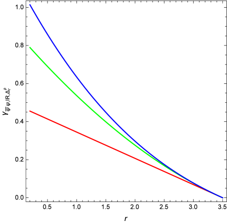
Figure 1: Plot of $\gamma_{\bar{\psi}\psi,IR,F,\Delta_{r}^{p}}$ as a function of $r$ in the $FR^{\prime}$ theory with $R^{\prime}=Adj$ and $N_{f^{\prime}}\equiv N_{Adj}=1$. From bottom to top, the curves (with colors online) refer to $\gamma_{\bar{\psi}\psi,IR,F,\Delta_{r}}$ (red), $\gamma_{\bar{\psi}\psi,IR,F,\Delta_{r}^{2}}$ (green) and $\gamma_{\bar{\psi}\psi,IR,F,\Delta_{r}^{3}}$ (blue).

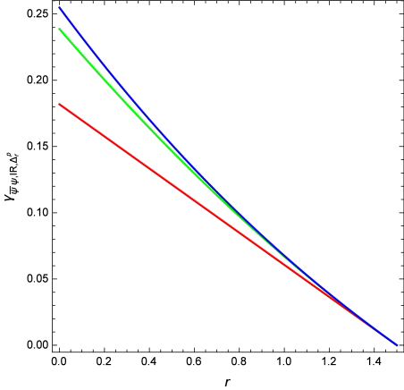
Figure 2: Plot of $\gamma_{\bar{\psi}\psi,IR,F,\Delta_{r}^{p}}$ as a function of $r$ in the $FR^{\prime}$ theory for the case $R^{\prime}=Adj$ and $N_{f^{\prime}}\equiv N_{Adj}=2$. From bottom to top, the curves (with colors online) refer to $\gamma_{\bar{\psi}\psi,IR,F,\Delta_{r}}$ (red), $\gamma_{\bar{\psi}\psi,IR,F,\Delta_{r}^{2}}$ (green) and $\gamma_{\bar{\psi}\psi,IR,F,\Delta_{r}^{3}}$ (blue).

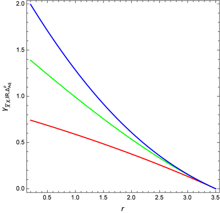
Figure 3: Plot of $\gamma_{\bar{\chi}\chi,IR,F,\check{\Delta}_{Adj}^{p}}$ as a function of $r$ in the $FR^{\prime}$ theory for the case $R^{\prime}=Adj$ and $N_{f^{\prime}}\equiv N_{Adj}=1$. From bottom to top, the curves (with colors online) refer to $\gamma_{\bar{\chi}\chi,IR,F,\check{\Delta}_{Adj}}$ (red), $\gamma_{\bar{\chi}\chi,IR,F,\check{\Delta}_{Adj}^{2}}$ (green) and $\gamma_{\bar{\chi}\chi,IR,F,\check{\Delta}_{Adj}^{3}}$ (blue).

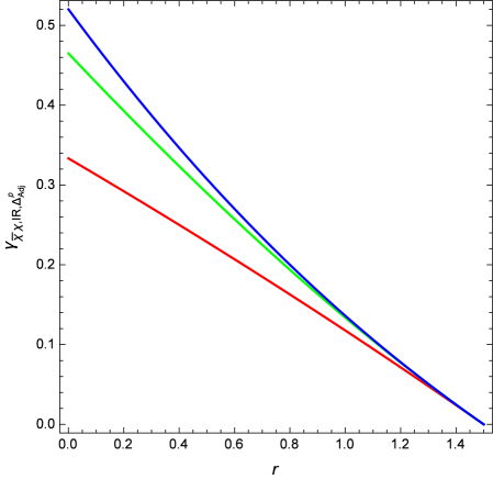
Figure 4: Plot of $\gamma_{\bar{\chi}\chi,IR,F,\check{\Delta}_{Adj}^{p}}$ as a function of $r$ in the $FR^{\prime}$ theory with $R^{\prime}=Adj$ and $N_{f^{\prime}}\equiv N_{Adj}=2$. From bottom to top, the curves (with colors online) refer to $\gamma_{\bar{\chi}\chi,IR,F,\check{\Delta}_{Adj}}$ (red), $\gamma_{\bar{\chi}\chi,IR,F,\check{\Delta}_{Adj}^{2}}$ (green) and $\gamma_{\bar{\chi}\chi,IR,F,\check{\Delta}_{Adj}^{3}}$ (blue).

We next insert these calculated coefficients $\hat{\kappa}^{(F)}_{j}$ and $\bar{\kappa}^{(Adj)}_{j}$ into the general scheme-independent expansions (25) for $f$ with $R=F$ and (26) for $f^{\prime}$. We show the results for $\gamma_{\bar{\psi}\psi,IR,\Delta_{r}^{p}}$ and $\gamma_{\bar{\chi}\chi,IR,\check{\Delta}_{Adj}^{p}}$ in Tables 4-7 for two illustrative cases, namely $R_{f^{\prime}}=Adj$, $N_{f^{\prime}}\equiv N_{Adj}=1$, and $N_{Adj}=2$. We present plots of $\gamma_{\bar{\psi}\psi,IR,\Delta_{r}^{p}}$ and $\gamma_{\bar{\chi}\chi,IR,\check{\Delta}_{r}^{p}}$ with $1\leq p\leq 3$ for these two theories in Figs. 1- 4.

It is of interest to compare the values of $\gamma_{\bar{\psi}\psi,IR,\Delta_{r}^{p}}$ and $\gamma_{\bar{\chi}\chi,IR,\check{\Delta}_{Adj}r^{p}}$ for $r=10/3$ with the results in the SU(3) theory with $N_{F}=10$, $R_{f^{\prime}}=Adj$, and $N_{f^{\prime}}=1$ given, respectively, in Tables V and VI of dexm . For that SU(3) theory one has $r=10/3$. In that theory, for the successive truncations to progressively high order for the scheme-independent series for $\gamma_{\bar{\psi}\psi,IR}$ we obtained $\gamma_{\bar{\psi}\psi,IR,\Delta_{F}}=0.0210$, $\gamma_{\bar{\psi}\psi,IR,\Delta_{F}^{2}}=0.0218$, and $\gamma_{\bar{\psi}\psi,IR,\Delta_{F}^{3}}=0.0218$, as listed in Table V of dexm . The LNN values that we have listed for $r=10/3$ in Table 4 are close to these for each order of truncation. In the above-mentioned SU(3) theory with $N_{F}=10$, $R_{f^{\prime}}=Adj$, and $N_{f^{\prime}}=1$ we calculated $\gamma_{\bar{\chi}\chi,IR,\Delta_{F}}=0.0.0466$, $\gamma_{\bar{\chi}\chi,IR,\Delta_{F}^{2}}=0.0490$, and $\gamma_{\bar{\chi}\chi,IR,\Delta_{F}^{3}}=0.0491$, as listed in Table V of dexm . Again, the LNN values that we have listed for $r=10/3$ in Table 5 are close to these for each order of truncation. This is in agreement with our general result that for even moderate values of $N_{c}$ and $N_{F}$ with $N_{F}/N_{c}=r$, and a given $R_{f^{\prime}}$ and $N_{f^{\prime}}$, the resulting anomalous dimensions are approximately given by the LNN limit with these values of $r$, $R_{f^{\prime}}$, and $N_{f^{\prime}}$, since correction terms to the LNN limit vanish rapidly, like $1/N_{c}^{2}$. As mentioned above, this was shown earlier for theories with fermions in a single representation of the gauge group, and our results here generalize this property to the LNN limit of the $FR^{\prime}$ theory.

IV LNN Limit for Scheme-Independent Beta Function Coefficients in $FR^{\prime}$ Theory

In the LNN limit, from dexm , we calculate

$$\hat{d}_{2}=\frac{2^{4}}{3^{2}(25+4\lambda_{f^{\prime}}N_{f^{\prime}})}$$ (53)

$$\hat{d}_{3}=\frac{2^{5}\cdot 13}{3^{3}(25+4\lambda_{f^{\prime}}N_{f^{\prime}})^{2}}$$ (54)

and

$$\hat{d}_{4} = \frac{2^{4}}{3^{5}(25+4\lambda_{f^{\prime}}N_{f^{\prime}})^{5}}\,\Bigg{[}2(183391-330000\zeta_{3})+2^{4}(1151+1800\zeta_{3})\lambda_{f^{\prime}}N_{f^{\prime}}$$ (55)

$$+ 2^{4}(-3161+3744\zeta_{3})(\lambda_{f^{\prime}}N_{f^{\prime}})^{2}+2^{8}(-23+24\zeta_{3})(\lambda_{f^{\prime}}N_{f^{\prime}})^{3}\Bigg{]}\ ,$$ (57)

where $\zeta_{s}=\sum_{n=1}^{\infty}n^{-s}$ is the Riemann zeta function. For the $\bar{d}_{j}$, we find

$$\bar{d}_{2}=\frac{2^{5}\lambda_{f^{\prime}}^{2}}{3^{2}(18-r)}$$ (58)

$$\bar{d}_{3}=\frac{2^{10}\lambda_{f^{\prime}}^{3}}{3^{3}(18-r)^{2}}$$ (59)

and

$$\bar{d}_{4}=\frac{2^{3}\lambda_{f^{\prime}}^{4}}{3^{5}(18-r)^{5}}\,\Bigg{[}3^{3}\cdot 46871+2^{2}\cdot 3^{4}(143-768\zeta_{3})r+2^{2}(-5153+6912\zeta_{3})r^{2}+2^{5}(23-24\zeta_{3})r^{3}\Bigg{]}\ .$$ (60)

We then substitute these results for $\hat{d}_{j}$ and $\bar{d}_{j}$ in Eqs. (40) and (41) with $f^{\prime}=Adj$, respectively, to obtain the series expansions for $\beta^{\prime}_{IR}$ in the theory with $R=F$ and $R^{\prime}=Adj$.

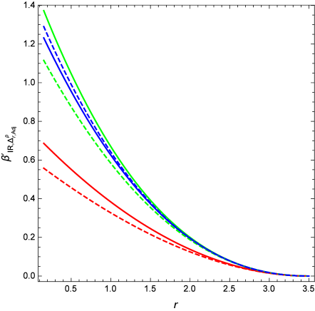
Figure 5: Plots of $\beta^{\prime}_{IR}$, as calculated with the expansion (36) (solid curves) and (37) (dashed curves) with $p=2,\ 3,\ 4$, as a function of $r$ in the $FR^{\prime}$ theory with $R^{\prime}=Adj$ and $N_{f^{\prime}}\equiv N_{Adj}=1$. The curves (with colors online) are as follows: $\beta^{\prime}_{IR,\Delta_{r}^{2}}$ (solid red), $\beta^{\prime}_{IR,\check{\Delta}_{Adj}^{2}}$ (dashed red), $\beta^{\prime}_{IR,\Delta_{r}^{3}}$ (solid green), $\beta^{\prime}_{IR,\check{\Delta}_{Adj}^{3}}$ (dashed green), $\beta^{\prime}_{IR,\Delta_{r}^{4}}$ (solid blue), and $\beta^{\prime}_{IR,\check{\Delta}_{Adj}^{4}}$ (dashed blue).

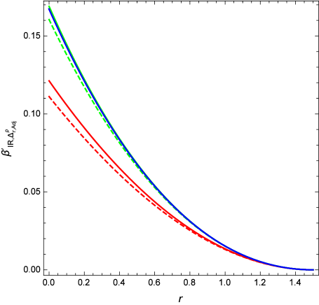
Figure 6: Plots of $\beta^{\prime}_{IR}$ as calculated with the expansion (36) (solid curves) and (37) (dashed curves) with $p=2,\ 3,\ 4$, as a function of $r$ in the $FR^{\prime}$ theory with $R^{\prime}=Adj$ and $N_{f^{\prime}}\equiv N_{Adj}=2$. The curves (with colors online) are as follows: $\beta^{\prime}_{IR,\Delta_{r}^{2}}$ (solid red), $\beta^{\prime}_{IR,\check{\Delta}_{Adj}^{2}}$ (dashed red), $\beta^{\prime}_{IR,\Delta_{r}^{3}}$ (solid green), $\beta^{\prime}_{IR,\check{\Delta}_{Adj}^{3}}$ (dashed green), $\beta^{\prime}_{IR,\Delta_{r}^{4}}$ (solid blue), and $\beta^{\prime}_{IR,\check{\Delta}_{Adj}^{4}}$ (dashed blue).

We present our results using the two equivalent scheme-independent series expansions for $\beta^{\prime}_{IR}$ in Tables 8 and 9 for our illustrative $FR^{\prime}$ theories in the LNN limit with $R_{f^{\prime}}\equiv R^{\prime}=Adj$ and $N_{Adj}=1$ and $N_{Adj}=2$, respectively, as a function of $r$. From left to right in these tables, the columns list $r$ and the successively higher truncations of the series expansions, namely $\beta^{\prime}_{IR,\Delta_{r}^{2}}$, $\beta^{\prime}_{IR,\check{\Delta}_{Adj}^{2}}$, $\beta^{\prime}_{IR,\Delta_{r}^{3}}$, $\beta^{\prime}_{IR,\check{\Delta}_{Adj}^{3}}$, $\beta^{\prime}_{IR,\Delta_{r}^{4}}$, and $\beta^{\prime}_{IR,\check{\Delta}_{Adj}^{4}}$. We see that for a given order $p$ of truncation, the alternate series expansion values $\beta^{\prime}_{IR,\Delta_{r}^{p}}$ and $\beta^{\prime}_{IR,\Delta_{Adj}^{p}}$ agree reasonably well with each other. This agreement improves as $r$ increases. In Figs. 5 and 6 we present plots of the expansions of $\beta^{\prime}_{IR}$ in powers of $\Delta_{r}$ and in powers of $\Delta_{Adj}$ for these $FR^{\prime}$ theories with $R^{\prime}=Adj$ and $N_{Adj}=1,\ 2$.

As before for the anomalous dimensions of fermion bilinears, it is of interest to compare these results in the LNN limit with the results from Ref. dexm for specific values of $N_{c}$ and $N_{F}$. Again, we pick $N_{c}=3$ and $N_{F}=10$, for which the appropriate comparison is with the LNN values with $r=10/3$. We can compare these with the values that we obtain in the LNN limit for the case $N_{Adj}=1$ (for $N_{Adj}=2$, this value of $r$ exceeds $r_{u}=3/2$). The values in the six columns of Table 8 for $r=10/3$ are $1.70\times 10^{-3}$, $1.68\times 10^{-3}$, $1.79\times 10^{-3}$, $1.79\times 10^{-3}$, $1.79\times 10^{-3}$, and $1.79\times 10^{-3}$, to be compared with the values in the corresponding six columns of Table IX of Ref. dexm , namely $1.75\times 10^{-3}$, $1.73\times 10^{-3}$, $1.84\times 10^{-3}$, $1.83\times 10^{-3}$, $1.84\times 10^{-3}$, and $1.84\times 10^{-3}$. One sees that for each entry in the respective columns of Table 8 and the corresponding Table IX in Ref. dexm the results are similar. As before, this shows the usefulness of the calculations in the LNN limit, since they approximately reproduce values of $\beta^{\prime}$ to a given order of truncation in the scheme-independent series expansions in an SU($N_{c}$) theory with $N_{F}$ fermions in the fundamental representation with $N_{F}/N_{c}$ equal to $r$. As was the case for the $\hat{\kappa}^{(F)}_{j}$ and $\bar{\kappa}^{(f^{\prime})}_{j}$, for large but finite $N_{f}$ and $N_{c}$, the approach to the LNN limit is rapid for the $\hat{d}_{j}$ and $\bar{d}_{j}$, since the subdominant terms again vanish like $1/N_{c}^{2}$.

V $AT$ Theory

In this section we analyze the large-$N_{c}$ limit of the $AT$ theory, i.e., a theory in which both the $f$ and $f^{\prime}$ fermions are in two-index representations of SU($N_{c}$). For finite $N_{c}$, there are two types of $AT$ theories, namely one with $R_{f}\equiv R=Adj$ and $R_{f^{\prime}}\equiv R^{\prime}=S_{2}$ and one with $R_{f}\equiv R=Adj$ and $R_{f^{\prime}}\equiv R^{\prime}=A_{2}$. Since the $S_{2}$ and $A_{2}$ representations have the same large-$N_{c}$ behavior, the $N_{c}\to\infty$ limits of both of these theories are the same, with $(R,R^{\prime})=(Adj,T_{2})$, where, as above, $T_{2}$ stands for either $S_{2}$ or $A_{2}$. This is the reason for our designation of these as the $AT$ theory. The fermions in the adjoint and $T_{2}$ representations are denoted $\psi$ and $\chi$.

V.1 Relevant Interval of $N_{Adj}$ and $N_{T_{2}}$ for $AT$ Theory

In the $N_{c}\to\infty$ limit of the $AT$ theory, the asymptotic freedom condition (6) reads

$$2N_{Adj}+N_{T_{2}}<\frac{11}{2}\ .$$ (61)

Hence, for a given value of $N_{Adj}$, $N_{T_{2}}$ must be less than the upper bound $N_{T_{2},u}=(11/2)-2N_{Adj}$, and for a given value of $N_{T_{2}}$, $N_{Adj}$ must be less than the upper bound $N_{Adj,u}=(11/4)-N_{T_{2}}/2$. Let us envision the theories as being specified by a point in the first quadrant, with the horizontal axis being $N_{Adj}$ and the vertical axis being $N_{T_{2}}$. The upper boundary of the conformal regime is defined by the line segment $N_{Adj}+(N_{T_{2}}/2)=11/4$. This line segment has slope

$$\frac{dN_{T_{2}}}{dN_{Adj}}=-2\ .$$ (62)

The expansion variables for the scheme-independent series expansions in the $AT$ theory are

$$\check{\Delta}_{Adj} = N_{Adj,u}-N_{Adj}$$ (63)

$$= \frac{11-2(2N_{Adj}+N_{T_{2}})}{4}$$ (65)

and

$$\check{\Delta}_{T_{2}} = N_{T_{2},u}-N_{T_{2}}$$ (66)

$$= \frac{11-2(2N_{Adj}+N_{T_{2}})}{2}\ ,$$ (68)

where the $\check{\Delta}$ notation signifies that we have taken the $N_{c}\to\infty$ limit. Thus,

$$\check{\Delta}_{T_{2}}=2\check{\Delta}_{Adj}\ .$$ (69)

As is evident from Eqs. (65) and (68), $\check{\Delta}_{T_{2}}$ and $\check{\Delta}_{Adj}$ depend on $N_{Adj}$ and $N_{T_{2}}$ only through the combination $2N_{Adj}+N_{T_{2}}$.

The condition that the two-loop beta function should have an IR zero is

$$2N_{Adj}+N_{T_{2}}>\frac{17}{8}\ .$$ (70)

The lower boundary of the region where the this condition (70) is satisfied is the line segment $2N_{Adj}+N_{T_{2}}=17/8$ in the first quadrant. This line segment has the same slope of $-2$ as the upper boundary. The region $I_{IRZ}$ is thus given by

$$I_{IRZ}:\quad\frac{17}{8}<2N_{Adj}+N_{T_{2}}<\frac{11}{2}\ .$$ (71)

For $N_{Adj}$ and $N_{T_{2}}$ in the IRZ region, the two-loop ($2\ell$) rescaled beta function $\beta_{\xi,2\ell}$ has an IR zero at

$$\xi_{IR,2\ell}=\frac{2\pi[11-2(2N_{Adj}+N_{T_{2}})]}{8(2N_{Adj}+N_{T_{2}})-17}\ .$$ (72)

Note that the upper and lower boundaries of the IRZ regime, the values of $\check{\Delta}_{T_{2}}$ and $\check{\Delta}_{Adj}$, and the value of $\xi_{IR,2\ell}$ depend on $N_{Adj}$ and $N_{T_{2}}$ only via the combination $2N_{Adj}+N_{T_{2}}$. We will assume that $N_{Adj}$ and $N_{T_{2}}$ are such that the theory has an IR zero in the conformal regime.

V.2 $\gamma_{Adj}$ and $\gamma_{T_{2}}$ in the $AT$ Theory

In the $AT$ theory, the coefficients of both types of fermions have finite large-$N_{c}$ limits, We denote $\kappa_{j}^{(f)}\equiv\kappa^{(Adj)}$ and $\kappa_{j}^{(f^{\prime})}\equiv\kappa^{(T_{2})}$. With $R_{2}$ standing for any of the three two-index representations $Adj$, $S_{2}$, and $A_{2}$, we define

$$\check{\kappa}^{(R_{2})}_{j}=\lim_{N_{c}\to\infty}\kappa^{(R_{2})}_{j}\quad{\rm for}\ R_{2}\ ,$$ (73)

so that

$$\gamma_{\bar{\psi}\psi,IR}=\sum_{j=1}^{\infty}\check{\kappa}^{(Adj)}_{j}\,\check{\Delta}_{Adj}^{j}$$ (74)

and

$$\gamma_{\bar{\chi}\chi,IR}=\sum_{j=1}^{\infty}\check{\kappa}^{(T_{2})}_{j}\,\check{\Delta}_{T_{2}}^{j}\ .$$ (75)

We find that for the $\kappa_{j}$ coefficients that we have calculated,

$$\check{\kappa}^{(T_{2})}_{j} = \bigg{(}\frac{\lambda_{T_{2}}}{\lambda_{Adj}}\bigg{)}^{j}\check{\kappa}^{(Adj)}_{j}$$ (76)

$$= 2^{-j}\,\check{\kappa}^{(Adj)}_{j}$$ (78)

From dexm , we have

$$\check{\kappa}^{(Adj)}_{1}=2\check{\kappa}^{(T_{2})}_{1}=\frac{2^{2}}{3^{2}}=0.444444$$ (79)

$$\check{\kappa}^{(Adj)}_{2}=2^{2}\check{\kappa}^{(T_{2})}_{2}=\frac{341}{2\cdot 3^{6}}=0.233882$$ (80)

$$\check{\kappa}^{(Adj)}_{3}=2^{3}\check{\kappa}^{(T_{2})}_{3}=\frac{61873}{2^{3}\cdot 3^{10}}=0.130978\ .$$ (81)

The large-$N_{c}$ limit for these coefficients in a theory with a single fermion representation $R=Adj$ was previously considered in Ref. dex , and the $\check{\kappa}^{(Adj)}_{j}$, $j=1,\ 2,\ 3$ agree with Eqs. (6.18)-(6.21) in that paper.

Combining the relation $\check{\Delta}_{T_{2}}=2\check{\Delta}_{Adj}$ from Eq. (69) with the relation $\check{\kappa}^{(T_{2})}_{j}=2^{-j}\,\check{\kappa}^{(Adj)}_{j}$ from Eq. (78), we derive an interesting symmetry property, namely that, for all the orders $p=1,\ 2,\ 3$ that we have calculated,

$$\gamma_{\bar{\psi}\psi,IR,\check{\Delta}_{Adj}^{p}}=\gamma_{\bar{\chi}\chi,IR,\check{\Delta}_{T_{2}}^{p}}\ .$$ (82)

That is, for the $\psi$ field in the $Adj$ representation and the $\chi$ field in either the $S_{2}$ or $A_{2}$ representation, the $N_{c}\to\infty$ limits of the scheme-independent series expansions for the anomalous dimensions of the corresponding bilinear operators, $\gamma_{\bar{\psi}\psi,IR}$ and $\gamma_{\bar{\chi}\chi,IR}$, are equal to each other at each order that we have calculated. Furthermore, since the only dependence on $N_{Adj}$ and $N_{T_{2}}$ enters via the combination $2N_{Adj}+N_{T_{2}}$, the anomalous dimensions in Eq. (82) also depend on $N_{Adj}$ and $N_{T_{2}}$ only through the combination $2N_{Adj}+N_{T_{2}}$. In Table 10 we list values of $\gamma_{\bar{\psi}\psi,IR,\check{\Delta}_{Adj}^{p}}=\gamma_{\bar{\chi}\chi,IR,\check{\Delta}_{T_{2}}^{p}}$ for $p=1,\ 2,\ 3$ in the $AT$ theory for some illustrative values of $N_{Adj}$ and $N_{T_{2}}$. As an example of the dependence on $2N_{Adj}+N_{T_{2}}$, the values of $\gamma_{\bar{\psi}\psi,IR,\check{\Delta}_{Adj}^{p}}$ for the theories with $(N_{Adj},N_{T_{2}})=(1,3)$ and $(N_{Adj},N_{T_{2}})=(2,1)$ are the same.

It is of interest to consider the correction terms to the $N_{c}\to\infty$ limit in this theory. The coefficients $\kappa^{(Adj)}_{j}$ with $j=1,2$ are independent of $N_{c}$ and hence are equal to their $N_{c}\to\infty$ limits $\check{\kappa}^{(Adj)}_{j}$ with $j=1,2$. For $\kappa^{(Adj)}_{3}$, in a theory with fermions in only a single representation, $R=Adj$, we recall that (see Eq. (6.20) in dex )

$$\kappa^{(Adj)}_{3}=\frac{61873-42624N_{c}^{-2}}{2^{3}\cdot 3^{10}}\quad(\rm one\ fermion\ rep.)\ ,$$ (83)

so the correction term to the $N_{c}\to\infty$ limit is proportional to $1/N_{c}^{2}$. In contrast, we find that the corrections to the $N_{c}\to\infty$ limits (79)-(81) in the $AT$ theory involve terms proportional to $1/N_{c}$ rather than $1/N_{c}^{2}$. Consequently, the approach to the $N_{c}=\infty$ limit in the $AT$ theory is slower than the approach to the LNN limit in the $FR^{\prime}$ theory, since in the latter case the correction terms are proportional to $1/N_{c}^{2}$.

V.3 $\beta^{\prime}_{IR}$ Series Expansions in the $AT$ Theory

In the $N_{c}\to\infty$ limit of the $AT$ theory, the coefficients $d_{j}$ and $\tilde{d}_{j}$ in the scheme-independent series expansions for $\beta^{\prime}_{IR}$ are finite. In accord with our labelling convention that $R_{f}=Adj$ and $R_{f^{\prime}}=T_{2}$, we denote $d_{j}\equiv d^{(Adj)}_{j}$ and $\tilde{d}_{j}\equiv d^{(T_{2})}_{j}$, and define

$$\check{d}^{(Adj)}_{j}=\lim_{N_{c}\to\infty}d^{(Adj)}_{j}$$ (84)

and

$$\check{d}^{(T_{2})}_{j}=\lim_{N_{c}\to\infty}d^{(T_{2})}_{j}\ ,$$ (85)

so that in this $N_{c}\to\infty$ limit, the two equivalent scheme-independent expansions for $\beta^{\prime}_{IR}$ are

$$\beta^{\prime}_{IR}=\sum_{j=2}^{\infty}\check{d}^{(Adj)}_{j}\check{\Delta}_{Adj}^{j}$$ (86)

and

$$\beta^{\prime}_{IR}=\sum_{j=2}^{\infty}\check{d}^{(T_{2})}_{j}\check{\Delta}_{T_{2}}^{j}\ .$$ (87)

For the cases $j=2,\ 3,\ 4$ that we have calculated, we find

$$\check{d}^{(T_{2})}_{j} = \bigg{(}\frac{\lambda_{T_{2}}}{\lambda_{Adj}}\bigg{)}^{j}\check{d}^{(Adj)}_{j}$$ (88)

$$= 2^{-j}\,\check{d}^{(Adj)}_{j}\ .$$ (90)

We calculate

$$\check{d}^{(Adj)}_{2}=2^{2}\check{d}^{(T_{2})}_{2}=\frac{2^{4}}{3^{4}}=0.197531\ ,$$ (91)

$$\check{d}^{(Adj)}_{3}=2^{3}\check{d}^{(T_{2})}_{3}=\frac{2^{8}}{3^{7}}=0.117055\ ,$$ (92)

$$\check{d}^{(Adj)}_{4}=2^{4}\check{d}^{(T_{2})}_{4}=\frac{46871}{2^{2}\cdot 3^{12}}=0.0220490\ .$$ (93)

Again, combining the relation $\check{\Delta}_{T_{2}}=2\check{\Delta}_{Adj}$ from Eq. (69) with the relation $\check{d}^{(T_{2})}_{j}=2^{-j}\,\check{d}^{(Adj)}_{j}$ from Eq. (90), we find a second symmetry property characterizing the $N_{c}\to\infty$ limit of the $AT$ theory, namely that, for all the orders $p=1,\ 2,\ 3$ that we have calculated,

$$\beta^{\prime}_{IR,\check{\Delta}_{Adj}^{p}}=\beta^{\prime}_{IR,\check{\Delta}_{T_{2}}^{p}}\ .$$ (94)

We thus write these as $\beta^{\prime}_{IR,\check{\Delta}_{R_{2}}^{p}}$, where $R_{2}$ stands for either $Adj$ or $T_{2}$. As discussed in dexm , these two scheme-independent expansions for $\beta^{\prime}_{IR}$ are equivalent, and here they are actually identically equal to each order that we have calculated. As was the case with the anomalous dimensions of the fermion bilinears, since the only dependence on $N_{Adj}$ and $N_{T_{2}}$ enters via the combination $2N_{Adj}+N_{T_{2}}$, the scheme-independent series expansion for $\beta^{\prime}$ depends on $N_{Adj}$ and $N_{T_{2}}$ only through the combination $2N_{Adj}+N_{T_{2}}$. In Table 11 we list values of $\beta^{\prime}_{IR,\check{\Delta}_{R_{2}}^{p}}$ for $p=2,\ 3,\ 4$ in the $AT$ theory for some illustrative values of $N_{Adj}$ and $N_{T_{2}}$. As another example of the dependence on $2N_{Adj}+N_{T_{2}}$, the values of $\beta^{\prime}_{IR,\check{\Delta}_{Adj}^{p}}$ for the theories with $(N_{Adj},N_{T_{2}})=(1,3)$ and $(N_{Adj},N_{T_{2}})=(2,1)$ are the same. As with the $\kappa^{(Adj)}_{j}$ and the $\kappa^{(T_{2})}_{j}$ coefficients, we find that the leading-order corrections to the $N_{c}\to\infty$ limit are proportional to $1/N_{c}$. In Figs.

VI Conclusions

In this paper we have calculated limiting forms of scheme-independent series expansions for the anomalous dimensions of gauge-invariant bilinear fermion operators and of $\beta^{\prime}$ evaluated at an infrared fixed point of the renormalization group in asymptotically free SU($N_{c})$ gauge theories. We have first studied a theory denoted $FR^{\prime}$ with $N_{F}$ fermions in the fundamental representation and $N_{f^{\prime}}$ fermions in the adjoint, or symmetric or antisymmetric rank-2 tensor representations, in the limit in which $N_{c}\to\infty$ and $N_{F}\to\infty$ with the ratio $r=N_{F}/N_{c}$ fixed and finite. Secondly, we have studied the $N_{c}\to\infty$ limit of a theory with fermions in the adjoint and symmetric or antisymmetric rank-2 tensor representations, denoted the $AT$ theory. We have shown how these limits yield useful simplifications of the general results in dexm . We have also determined the nature of the approaches to the respective LNN and $N_{c}\to\infty$ limits in the $FR^{\prime}$ and $AT$ theories. Our results further elucidate the interesting and fundamental question of the properties of a conformal field theory, s pecifically, an asymptotically free gauge theory at a conformal infrared fixed point of the renormalization group

Table 1: Values of $r_{\ell}$ and $r_{u}$ as functions of $N_{f^{\prime}}$ for $R^{\prime}=Adj$ and $R^{\prime}=T_{2}$ ($S_{2}$ or $A_{2}$) in the LNN limit of the $FR^{\prime}$ theory. As noted in the text, since the adjoint representation is self-conjugate, half-integral values of $N_{Adj}$ are allowed, corresponding to $2N_{Adj}$ Majorana fermions.

$R^{\prime}$	$r_{\ell}$	$r_{u}$
$N_{Adj}=1/2$	1.385	4.50
$N_{Adj}=1$	0.154	3.50
$N_{Adj}=3/2$	0	2.50
$N_{Adj}=2$	0	1.50
$N_{T_{2}}=1$	1.385	4.50
$N_{T_{2}}=2$	0.154	3.50
$N_{T_{2}}=3$	0	2.50
$N_{T_{2}}=4$	0	1.50
$N_{T_{2}}=5$	0	0.50

Table 2: Values of $\hat{\kappa}^{(F)}_{j}$ with $j=1,\ 2,\ 3$ in the LNN limit of the $FR^{\prime}$ theory with $R^{\prime}=Adj$, as a function of $N_{Adj}$. (As noted in the text, since the adjoint representation is self-conjugate, half-integral values of $N_{Adj}$ are allowed, corresponding to $2N_{Adj}$ Majorana fermions.) The notation $a$e-n means $10^{-n}$. See Table 1 for relevant ranges of $N_{Adj}$ as a function of $r$.

$N_{Adj}$	$\hat{\kappa}^{(F)}_{1}$	$\hat{\kappa}^{(F)}_{2}$	$\hat{\kappa}^{(F)}_{3}$
1/2	0.148	0.0339	0.718e-2
1	0.138	0.0307	0.642e-2
3/2	0.129	0.0278	0.546e-2
2	0.121	0.0253	0.480e-2

Table 3: Values of $\bar{\kappa}^{(Adj)}_{j}$ with $j=1,\ 2,\ 3$ in the LNN limit of the $FR^{\prime}$ theory with $R^{\prime}=Adj$ and $N_{Adj}=1$, as a function of $r$. See Table 1 for relevant ranges of $r$ as a function of $N_{Adj}$.

$r$	$\bar{\kappa}^{(Adj)}_{1}$	$\bar{\kappa}^{(Adj)}_{2}$	$\bar{\kappa}^{(Adj)}_{3}$
0.2	0.449	0.238	0.1345
0.4	0.4545	0.243	0.138
0.6	0.460	0.248	0.142
0.8	0.465	0.253	0.146
1.0	0.471	0.2575	0.150
1.2	0.476	0.263	0.154
1.4	0.482	0.268	0.159
1.6	0.488	0.273	0.163
1.8	0.494	0.279	0.168
2.0	0.500	0.285	0.173
2.2	0.506	0.291	0.178
2.4	0.513	0.297	0.178
2.6	0.519	0.303	0.189
2.8	0.526	0.310	0.194
3.0	0.533	0.316	0.200
3.2	0.541	0.323	0.206
3.4	0.548	0.330	0.213

Table 4: Values of the anomalous dimension $\gamma_{\bar{\psi}\psi,IR,\Delta_{r}^{p}}$, calculated to order $p=1,\ 2,\ 3$ and evaluated at the IR fixed point in the LNN limit of the $FR^{\prime}$ theory with $R^{\prime}=Adj$ and $N_{Adj}=1$, as a function of $r$. Here, $\Delta_{r}=(7-2r)/2$ and $\psi$ is the fermion in the $F$ representation. See Table 1 for relevant range of $r$. See text for further discussion.

$r$	$\gamma_{\bar{\psi}\psi,IR,\Delta_{r}}$	$\gamma_{\bar{\psi}\psi,IR,\Delta_{r}^{2}}$	$\gamma_{\bar{\psi}\psi,IR,\Delta_{r}^{3}}$
0.2	0.455	0.789	1.014
0.4	0.428	0.722	0.908
0.6	0.400	0.658	0.810
0.8	0.372	0.596	0.719
1.0	0.345	0.5365	0.634
1.2	0.317	0.479	0.555
1.4	0.290	0.425	0.483
1.6	0.262	0.373	0.416
1.8	0.234	0.323	0.354
2.0	0.207	0.276	0.297
2.2	0.179	0.231	0.245
2.4	0.152	0.189	0.197
2.6	0.124	0.149	0.154
2.8	0.0966	0.112	0.114
3.0	0.0690	0.0766	0.0774
3.2	0.0414	0.0441	0.0443
3.333	0.0230	0.0238	0.0239
3.4	0.01379	0.01410	0.01411

Table 5: Values of the anomalous dimension $\gamma_{\bar{\chi}\chi,IR,\Delta_{F}^{p}}$, calculated to order $p=1,\ 2,\ 3$ and evaluated at the IR fixed point in the LNN limit of the $FR^{\prime}$ theory with $R^{\prime}=Adj$ and $N_{Adj}=1$, as a function of value of $r$. Here, $\check{\Delta}_{Adj}=(7-2r)/4$, and $\chi$ is the fermion in the $Adj$ representation. See text for further discussion.

$r$	$\gamma_{\bar{\chi}\chi,IR,\check{\Delta}_{Adj}}$	$\gamma_{\bar{\chi}\chi,IR,\check{\Delta}_{Adj}^{2}}$	$\gamma_{\bar{\chi}\chi,IR,\check{\Delta}_{Adj}^{3}}$
0.2	0.742	1.390	1.995
0.4	0.705	1.288	1.803
0.6	0.667	1.187	1.620
0.8	0.628	1.088	1.447
1.0	0.588	0.991	1.284
1.2	0.548	0.895	1.130
1.4	0.506	0.801	0.985
1.6	0.463	0.710	0.850
1.8	0.420	0.621	0.724
2.0	0.375	0.535	0.608
2.2	0.329	0.452	0.501
2.4	0.282	0.372	0.402
2.6	0.234	0.295	0.312
2.8	0.184	0.222	0.230
3.0	0.133	0.153	0.156
3.2	0.0811	0.0884	0.0891
3.333	0.04545	0.0477	0.04785
3.4	0.02740	0.02822	0.02825

Table 6: Values of the anomalous dimension $\gamma_{\bar{\psi}\psi,IR,\Delta_{r}^{p}}$, calculated to order $p=1,\ 2,\ 3$ and evaluated at the IR fixed point in the LNN limit of the $FR^{\prime}$ theory with $R^{\prime}=Adj$ and $N_{Adj}=2$, as a function of $r$. Here, $\Delta_{r}=(3-2r)/2$ and $\psi$ is the fermion in the $F$ representation. See Table 1 for relevant range of $r$. See text for further discussion.

$r$	$\gamma_{\bar{\psi}\psi,IR,\Delta_{r}}$	$\gamma_{\bar{\psi}\psi,IR,\Delta_{r}^{2}}$	$\gamma_{\bar{\psi}\psi,IR,\Delta_{r}^{3}}$
0.2	0.158	0.200	0.211
0.4	0.133	0.164	0.170
0.6	0.109	0.130	0.133
0.8	0.0848	0.0972	0.0989
1.0	0.0606	0.0669	0.0675
1.2	0.0364	0.0386	0.0388
1.4	0.0121	0.0124	0.0124

Table 7: Values of the anomalous dimension $\gamma_{\bar{\chi}\chi,IR,\check{\Delta}_{Adj}^{p}}$, calculated to order $p=1,\ 2,\ 3$ and evaluated at the IR fixed point in the LNN limit of the $FR^{\prime}$ theory with $R^{\prime}=Adj$ and $N_{Adj}=2$, as a function of value of $r$. Here, $\check{\Delta}_{Adj}=(3-2r)/4$, and $\chi$ is the fermion in the $Adj$ representation. See text for further discussion.

$r$	$\gamma_{\bar{\chi}\chi,IR,\check{\Delta}_{Adj}}$	$\gamma_{\bar{\chi}\chi,IR,\check{\Delta}_{Adj}^{2}}$	$\gamma_{\bar{\chi}\chi,IR,\check{\Delta}_{Adj}^{3}}$
0.2	0.292	0.393	0.430
0.4	0.250	0.323	0.430
0.6	0.207	0.257	0.270
0.8	0.163	0.194	0.200
1.0	0.118	0.134	0.136
1.2	0.0714	0.0773	0.0779
1.4	0.0241	0.0248	0.0248

Table 8: Values of $\beta^{\prime}_{IR}$ as calculated to order $O(\Delta_{r}^{p})$ via Eq. (40), denoted $\beta^{\prime}_{IR,\Delta_{r}^{p}}$ and to order $O(\check{\Delta}_{Adj}^{p})$ via Eq. (41), denoted $\beta^{\prime}_{IR,\Delta_{Adj}^{p}}$, with $p=2,\ 3,\ 4$, in the LNN limit of the $FR^{\prime}$ theory with $R^{\prime}=Adj$ and $N_{Adj}=1$, as functions of $r$. Here $\Delta_{r}=2\check{\Delta}_{Adj}=(7-2r)/2$. The notation $a$e-n means $a\times 10^{-n}$.

$r$	$\beta^{\prime}_{IR,\Delta_{r}^{2}}$	$\beta^{\prime}_{IR,\check{\Delta}_{Adj}^{2}}$	$\beta^{\prime}_{IR,\Delta_{r}^{3}}$	$\beta^{\prime}_{IR,\check{\Delta}_{Adj}^{3}}$	$\beta^{\prime}_{IR,\Delta_{r}^{4}}$	$\beta^{\prime}_{IR,\check{\Delta}_{Adj}^{4}}$
0.2	0.668	0.544	1.326	1.0815	1.192	1.2475
0.4	0.589	0.485	1.135	0.941	1.031	1.0725
0.6	0.516	0.430	0.962	0.8115	0.883	0.9136
0.8	0.447	0.377	0.807	0.692	0.748	0.770
1.0	0.383	0.327	0.669	0.583	0.625	0.641
1.2	0.324	0.280	0.547	0.484	0.516	0.526
1.4	0.270	0.236	0.440	0.395	0.418	0.425
1.6	0.221	0.196	0.347	0.317	0.332	0.337
1.8	0.177	0.159	0.267	0.247	0.258	0.260
2.0	0.138	0.125	0.200	0.1875	0.194	0.1955
2.2	0.104	0.0951	0.144	0.137	0.141	0.141
2.4	0.0742	0.0689	0.0986	0.0949	0.0969	0.09275
2.6	0.0497	0.04675	0.0630	0.0613	0.0623	0.0624
2.8	0.0300	0.0287	0.0363	0.0357	0.03605	0.0361
3.0	0.0153	0.0148	0.0176	0.0174	0.0175	0.01755
3.2	0.552e-2	0.5405e-2	0.601e-2	0.599e-2	0.600e-2	0.600e-3
3.333	1.70e-3	1.68e-3	1.79e-3	1.79e-3	1.79e-3	1.79e-3
3.4	0.613e-3	0.609e-3	0.631e-3	0.631e-3	0.631e-3	0.631e-3

Table 9: Values of $\beta^{\prime}_{IR}$ as calculated to order $O(\Delta_{r}^{p})$ via Eq. (40), denoted $\beta^{\prime}_{IR,\Delta_{r}^{p}}$ and to order $O(\Delta_{Adj}^{p})$ via Eq. (41), denoted $\beta^{\prime}_{IR,\check{\Delta}_{Adj}^{p}}$, with $p=2,\ 3,\ 4$, in the LNN limit of the $FR^{\prime}$ theory with $R^{\prime}=Adj$ and $N_{Adj}=2$, as functions of $r$. Here $\Delta_{r}=2\check{\Delta}_{Adj}=(3-2r)/2$. The notation $a$e-n means $a\times 10^{-n}$.

$r$	$\beta^{\prime}_{IR,\Delta_{r}^{2}}$	$\beta^{\prime}_{IR,\check{\Delta}_{Adj}^{2}}$	$\beta^{\prime}_{IR,\Delta_{r}^{3}}$	$\beta^{\prime}_{IR,\check{\Delta}_{Adj}^{3}}$	$\beta^{\prime}_{IR,\Delta_{r}^{4}}$	$\beta^{\prime}_{IR,\check{\Delta}_{Adj}^{4}}$
0.2	0.0910	0.0844	0.122	0.117	0.121	0.121
0.4	0.0652	0.0611	0.0840	0.0815	0.0835	0.0836
0.6	0.0436	0.0414	0.05395	0.0528	0.0537	0.0537
0.8	0.0264	0.0253	0.03125	0.0308	0.0312	0.0312
1.0	0.0135	0.0137	0.0152	0.151	0.0152	0.0152
1.2	0.485e-2	0.476e-2	0.523e-2	0.522e-2	0.523e-2	0.523e-2
1.4	0.539e-3	0.535e-3	0.553e-3	0.553e-3	0.0553e-3	0.553e-3

Table 10: Values of the anomalous dimension $\gamma_{\bar{\psi}\psi,IR,\check{\Delta}_{Adj}^{p}}=\gamma_{\bar{\chi}\chi,IR,\check{\Delta}_{T_{2}}^{p}}$, calculated to order $p=1,\ 2,\ 3$ and evaluated at the IR fixed point in the $AT$ theory for illustrative values of $N_{Adj}$ and $N_{T_{2}}$. The respective entries are identical for the $(N_{Adj},N_{T_{2}})=(1,3)$ and $(2,1)$, and hence the latter are not shown.

$N_{Adj}$	$N_{T_{2}}$	$2N_{Adj}+N_{T_{2}}$	$\gamma_{\bar{\psi}\psi,IR,\check{\Delta}_{Adj}}$	$\gamma_{\bar{\psi}\psi,IR,\check{\Delta}_{Adj}^{2}}$	$\gamma_{\bar{\psi}\psi,IR,\check{\Delta}_{Adj}^{3}}$
1	2	4	0.333	0.465	0.520
1	3	5	0.111	0.126	0.128

Table 11: Values of $\beta^{\prime}_{IR}$ as calculated to order $O(\check{\Delta}_{Adj}^{p})$, denoted $\beta^{\prime}_{IR,\check{\Delta}_{Adj}^{p}}$ and to order $O(\check{\Delta}_{T_{2}}^{p})$, denoted $\beta^{\prime}_{IR,\check{\Delta}_{T_{2}}^{p}}$, with $p=2,\ 3,\ 4$, in the AT theory for illustrative values of $N_{Adj}$ and $N_{T_{2}}$. As discussed in the text, $\beta^{\prime}_{IR,\check{\Delta}_{Adj}^{p}}=\beta^{\prime}_{IR,\check{\Delta}_{T_{2}}^{p}}$, so we denote these as $\beta^{\prime}_{IR,\check{\Delta}_{R_{2}}^{p}}$, where $R_{2}$ stands for either $Adj$ or $T_{2}$. The respective entries are identical for the $(N_{Adj},N_{T_{2}})=(1,3)$ and $(2,1)$, and hence the latter are not shown.

$N_{Adj}$	$N_{T_{2}}$	$2N_{Adj}+N_{T_{2}}$	$\beta^{\prime}_{IR,\check{\Delta}_{R_{2}}^{2}}$	$\beta^{\prime}_{IR,\check{\Delta}_{R_{2}}^{3}}$	$\beta^{\prime}_{IR,\check{\Delta}_{R_{2}}^{4}}$
1	2	4	0.111	0.1605	0.1675
1	3	5	0.0123	0.0142	0.0143

References

• (1) T. A. Ryttov and R. Shrock, Phys. Rev. D 98, 096003 (2018) [arXiv:1809.02242].
• (2) Taking the fermions to be massless does not involve any loss of generality, because a fermion with a nonzero mass $m_{0}$ would be integrated out of the low-energy effective field theory at Euclidean momentum scales $\mu<m_{0}$, and hence would not affect the properties of the theory at the IRFP.
• (3) R. Shrock, Phys. Rev. D 87, 105005 (2013) [arXiv:1301.3209]; Phys. Rev. D 87, 116007 (2013) [arXiv:1302.5434].
• (4) T. A. Ryttov and R. Shrock, Phys. Rev. D 94, 125005 (2016) [arXiv:1610.00387].
• (5) T. A. Ryttov and R. Shrock, Phys. Rev. D 95, 105004 (2017) [arXiv:1703.08558].
• (6) For recent reviews of these lattice simulations, see, e.g., talks in the Lattice for BSM 2017 Workshop at http://www-hep.colorado.edu/(tilde)eneil/lbsm17; Lattice-2017 at http://wpd.ugr.es/(tilde)lattice2017; simons ; and Lattice-2018 at https://web.pa.msu.edu/conf/Lattice2018.
• (7) Simons Workshop on Continuum and Lattice Approaches to the Infrared Behavior of Conformal and Quasiconformal Gauge Theories, Jan. 8-12, 2018, T. A. Ryttov and R. Shrock, organizers; http://scgp.stonybrook.edu/archives/21358.
• (8) J. Polchinski, Nucl. Phys. B 303, 226 (1988); J.-F. Fortin, B. Grinstein and A. Stergiou, JHEP 01 (2013) 184 (2013); A. Dymarsky, Z. Komargodski, A. Schwimmer, and S. Thiessen, JHEP 10, 171 (2015) and references therein.
• (9) T. A. Ryttov, R. Shrock, Phys. Rev. D 83, 056011 (2011) [arXiv:1011.4542].
• (10) C. Pica, F. Sannino, Phys. Rev. D 83, 035013 (2011) [arXiv:1011.5917].
• (11) T. A. Ryttov and R. Shrock, Phys. Rev. D 96, 105018 (2017) [arXiv:1706.06422]; Phys. Rev. D 97, 065020 (2018) [arXiv:1711.01116].
• (12) T. A. Ryttov, Phys. Rev. Lett. 117, 071601 (2016) [arXiv:1604.00687].
• (13) T. A. Ryttov and R. Shrock, Phys. Rev. D 94, 105014 (2016) [arXiv:1608.00068].
• (14) T. A. Ryttov and R. Shrock, Phys. Rev. D 96, 105015 (2017) [arXiv:1709.05358].
• (15) T. A. Ryttov and R. Shrock, Phys. Rev. D 97, 025004 (2018) [arXiv:1710.06944].
• (16) In Eqs. (3.3) and (5.7) of dex , $b_{\ell}^{(r)}$ should be $((-1)^{r}/r!)b_{\ell}^{(r)}$ and in Eq. (4.5), $c_{{\cal O},\ell}^{(r)}$ should be $((-1)^{r}/r!)c_{{\cal O},\ell}^{(r)}$. These were just switches in notation in the text and did not affect the calculations or results.
• (17) T. Banks and A. Zaks, Nucl. Phys. B 196, 189 (1982).
• (18) T. van Ritbergen, J. A. M. Vermaseren, and S. A. Larin, Phys. Lett. B 400, 379 (1997).
• (19) P. A. Baikov, K. G. Chetyrkin, and J. H. KΓΌhn, Phys. Rev. Lett. 118, 082002 (2017).
• (20) F. Herzog, B. Ruijl, T. Ueda, J. A. M. Vermaseren, and A. Vogt, JHEP 02 (2017) 090.
• (21) . K. G. Chetyrkin, Phys. Lett. B 404, 161 (1997); J. A. M. Vermaseren, S. A. Larin, and T. van Ritbergen, Phys. Lett. B 405, 327 (1997).
• (22) M. F. Zoller, JHEP 10, 118 (2016) [arXiv:1608.08982].
• (23) K. G. Chetyrkin and M. F. Zoller, JHEP 06, 074 (2017) [arXiv:1704.04209].
• (24) We recall the general definitions of these group invariants. Denote $T_{R}$ as a generator of the Lie algebra of a group $G$. Then the quadratic Casimir invariant $C_{2}(R)$ is defined by $T^{a}_{R}T^{a}_{R}=C_{2}(R)I$, where $I$ is the $d_{R}\times d_{R}$ identity matrix, and the trace invariant $T(R)$ is defined by ${\rm Tr}_{R}(T^{a}_{R}T^{b}_{R})=T(R)\delta_{ab}$, where $1\leq a\leq o(G)$, with $o(G)$ the order of the group. We write $C_{A}=C_{2}(Adj)$, $C_{f}=C_{2}(R_{f})$, and $C_{f^{\prime}}=C_{2}(R_{f^{\prime}})$. For SU($N_{c}$), $C_{2}(Adj)=T(Adj)=N_{c}$; $C_{2}(T_{2})=(N_{c}\pm 2)(N_{c}\mp 1)/N_{c}$; and $T(T_{2})=(N_{c}\pm 2)/2$, where the $+$ and $-$ signs apply for $T_{2}=S_{2}$ and $A_{2}$, respectively.
• (25) J. A. Gracey, Phys. Lett. B 488, 175 (2000).
• (26) V. Ayyar, T. DeGrand, M. Golterman, D. Hackett, W. I. Jay, E. T. Neil, Y. Shamir, and B. Svetitsky, Phys. Rev. D 97, 074505 (2016) [arXiv:1710.00806].
• (27) V. Ayyar, T. DeGrand, D. Hackett, W. I. Jay, E. T. Neil, Y. Shamir, and B. Svetitsky, Phys. Rev. D 97, 114505 (2018) [arXiv:1801.05809]; Phys. Rev. D 97, 114502 (2018) [arXiv:1802.09644].