Cosmic distance determination from photometric redshift samples using BAO peaks only

Abstract

The galaxy distributions along the line-of-sight are significantly contaminated by the uncertainty on redshift measurements obtained through multiband photometry, which makes it difficult to get cosmic distance information measured from baryon acoustic oscillations, or growth functions probed by redshift distortions. We investigate the propagation of the uncertainties into large scale clustering by exploiting all known estimators, and propose the wedge approach as a promising analysis tool to extract cosmic distance information still remaining in the photometric galaxy samples. We test our method using simulated galaxy maps with photometric uncertainties of $\sigma_{0}=\left(0.01,0.02,0.03\right)$. The measured anisotropy correlation function $\xi$ is binned into the radial direction of $s$ and the angular direction of $\mu$, and the variations of $\xi(s,\mu)\,$with perpendicular and radial cosmic distance measures of $D_{A}$ and $H^{-1}$ are theoretically estimated by an improved RSD model. Although the radial cosmic distance $H^{-1}$ is unable to be probed from any of the three photometric galaxy samples, the perpendicular component of $D_{A}$ is verified to be accurately measured even after the full marginalisation of $H^{-1}$. We measure $D_{A}$ with approximately 6% precision which is nearly equivalent to what we can expect from spectroscopic DR12 CMASS galaxy samples.

1 Introduction

Since the discovery of the cosmic acceleration (Riess et al., 1998; Perlmutter et al., 1999), many theoretical models have been proposed to explain the cause of it by introducing a positive cosmological constant, a time varying dark energy component, or a modified theory of gravity. As most ongoing observations support the $\Lambda$CDM model with the presence of the cosmological constant, it becomes an interesting observational mission to confirm $\Lambda$CDM in high precision, or to probe any possible deviation from it. The expansion history of the Universe can be revealed by diverse cosmic distance measures in tomographic redshift space, such as cosmic parallax (Benedict et al., 1999), standard candles (Fernie, 1969) or standard rulers (Eisenstein et al., 1998, 2005), and the possible presence of dynamical dark energy evolution can be confirmed or excluded in precision.

The tension between gravitational infall and radiative pressure caused by the baryon-photon fluid in the early Universe gave rise to an acoustic peak structure which was imprinted on the last-scattering surface (hereafter BAO) (Peebles & Yu, 1970). BAO is known as a relatively risk free standard ruler technique to probe cosmic distances. The BAO feature has been measured through the correlation function (Blake & Glazebrook, 2003; Eisenstein et al., 2005), and the most successful measurements in the clustering of large-scale structure at low redshifts have been obtained using data from SDSS (Eisenstein et al., 2005; Estrada et al., 2009; Padmanabhan et al., 2012; Hong et al., 2012; Veropalumbo et al., 2014, 2016; Alam et al., 2017). In the near future, the wider and deeper Dark Energy Spectroscopic Instrument (hereafter DESI) survey will be launched to probe the earlier expansion history with greater precision using spectroscopic redshifts. However, the footprint photometric survey for DESI has already been completed. Although these photometric redshifts are measured with a much poorer resolution, there might still be possible BAO signatures that have not been contaminated by the redshift uncertainty. If that is the case, we should be able to provide the precursor of cosmic distance information which will be revealed by the follow up spectroscopy experiment much later on. We investigate the optimised methodology to extract the uncontaminated cosmic distance information in the photometric data sets. This statistical tool can also be applicable for many imaging surveys, such as the the ongoing Dark Energy Survey (The Dark Energy Survey Collaboration, 2005), the PAUS survey (Benítez et al., 2009; Padilla et al., 2019), the Javalambre Physics of the Accelarating Universe Astrophysical survey (JPAS) (Benitez et al., 2014) or upcoming surveys such as Large Synoptic Survey Telescope (Ivezic et al., 2008; LSST Science Collaboration et al., 2009) and Euclid (Laureijs et al., 2011).

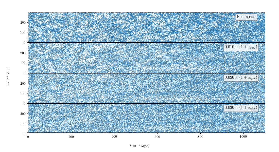
Figure 1: The galaxy distributions with varying uncertainties of $z$ measurement are presented along the transverse and radial directions. The maps with different $z$ dispersion of $\sigma_{0}=(0,0.01,0.02,0.03)$ are shown from the top to the bottom panels. Here $Y$ and $Z$ denote the transverse and radial coordinates respectively.

It is known that the correlation along the line-of-sight (hereafter LOS) is obtained with precise spectroscopic redshift measurements with the dispersion being in the order of $\sigma_{z}/(1+z)<0.001$. This dispersion has decreased with state-of-the-art spectrograph design with the upcoming DESI survey (DESI Collaboration et al., 2016) which is expected to have $\sigma_{z}/(1+z)\sim 0.0005$, but such surveys are time consuming. If the imaging survey is done with multiple bands, then the photometric redshifts can be estimated as precise as $\sigma_{z}/(1+z)>0.01$. It has been recently shown by the Physics of the Accelerating Universe Survey (PAUS) that by using a filter system with 40 filters, each with a width close to 100$\mathrm{\SIUnitSymbolAngstrom}$, the redshifts dispersion can be further reduced to $\sigma_{z}/(1+z)\sim 0.003$ (Benítez et al., 2009; Martí et al., 2014). The ongoing Dark Energy Survey aims to cover about 5000 deg² of the sky with a photometric accuracy of $\sigma_{z}\approx 0.08$ out to $z\approx 1$ (Sánchez et al., 2014b). Future surveys such as LSST and Euclid are expected to make a significant leap forward. The Euclid Wide Survey, planned to cover 15000 deg², is expected to deliver photometric redshifts with uncertainties lower than $\sigma_{z}/(1+z)<0.05$, and possibly $\sigma_{z}/(1+z)<0.03$, over the redshift range [0,2] (Laureijs et al., 2011). While the photo-z survey provides more observed galaxies compared to a spectroscopic survey even at deeper redshifts, an unpredictable damping of clustering at small scales and a smearing of the BAO peak is caused by the photo-z uncertainty (Estrada et al., 2009). Thus the cosmological information contained in the large-scale clustering is expected to be significantly contaminated. However, the cosmic distance obtainable using the correlated clustering at the perpendicular direction can be least contaminated by this uncertainty, and there will be a way to separately extract this remaining information from other contaminated parts along the LOS. We apply the wedge approach (Kazin et al., 2013; Sánchez et al., 2014a; Sabiu & Song, 2016; Ross et al., 2017; Sánchez et al., 2017) to probe the uncontaminated BAO feature by binning the angular direction from the perpendicular to radial directions, and try to successfully recover the residual BAO peak that has survived and get constraints on $D_{A}$ and $H^{-1}$. Recovering the real-space correlation function at small scales ($s<50\,\mathrm{h}^{-1}\mathrm{Mpc}$) has been done recently using the deprojection method by Sridhar et al. (2017), but it is of major interest to check the impact of this effect on the BAO peak when using photo-z’s.

The paper is described as follows: In Section 2 we describe the different correlation functions we calculate and introduce the catalogue which we use for the analysis. In Section 3 we describe the theoretical RSD model that we use to get the correlation function at the targeted redshift and analyse the BAO peak obtained from $\xi(s,\mu)\,$. We also compare the 68% and 95% confidence limits on the fiducial values of $D_{A}$ and $H^{-1}$ obtained from the spectroscopic and photometric samples. We summarise all our results in Section 4.

2 Remaining BAO feature in photometric map

The excess probability of finding two objects relative to a Poisson distribution at volumes $dV_{1}$ and $dV_{2}$ separated by a vector distance r is given by the two-point correlation function $\xi(r)$ (Totsuji & Kihara, 1969; Davis & Peebles, 1983). The galaxy distribution seen in redshift space exhibits an anisotropic feature distorting $\xi(r)$ into $\xi(\sigma,\pi)$ along the LOS where $\sigma$ and $\pi$ denote the transverse and radial components of the separation vector r. Acoustic fluctuations of the baryon–radiation plasma of the primordial Universe leaves the signature on the density perturbation of baryons. This standard ruler length scale, set by the acoustic wave, propagates until it is frozen at decoupling epoch to remain in the large scale structure of the Universe. The threshold length scale of acoustic wave is called as the sound horizon, which is given by,

$$r_{s}=\int_{z_{drag}}^{\infty}\frac{c_{s}(z)}{H(z)}dz$$ (1)

where $c_{s}$ is sound speed of the plasma. In a wide deep field spectroscopic galaxy survey, the signature of the BAO wave is observed in precisely determined redshift space, which opens an opportunity to separately access transverse and radial cosmic distances. If the target galaxy distribution is given by photometrically determined redshift, then it is expected that both measured distances are differently contaminated by the uncertainty in redshift determination. We present diverse correlation function estimators below, and find an optimal one to probe the least contaminated distance measure.

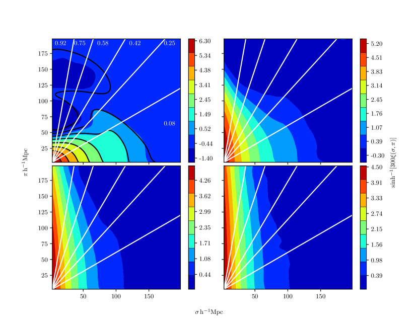
Figure 2: The two-dimensional correlation function for the spectroscopic sample (top left), $\sigma_{0}=0.01\,$photometric sample (top right), $\sigma_{0}=0.02\,$photometric sample (bottom left) and $\sigma_{0}=0.03\,$photometric sample (bottom right) given by the coloured contours. The BAO feature which is clearly visible in the spectroscopic sample ($\sim 100\,\mathrm{h}^{-1}\mathrm{Mpc}$) is smoothed out in the photometric samples (the smoothing becomes greater with increasing photometric uncertainty). The function plotted in the colour bar is sinh${}^{-1}(300)\xi(\sigma,\pi)$, which is linear near zero, but logarithmic for high values of $\xi(\sigma,\pi)$. The solid black line in the top left panel is the $\xi(\sigma,\pi)\,$calculated (at the same redshift as the sample) from the theoretical model explained in Section 3.1. The solid white lines denote the different $\mu$ bins in which we calculate $\xi(s,\mu)\,$and the mean values of each $\mu$ bin is written in white. Units on both the axes are in $\mathrm{h}^{-1}$Mpc.

2.1 The simulated photometric map

The photometric galaxy distribution simulations are made using 1000 simulations mocking the galaxy distributions and survey geometry of DR12 CMASS catalogue (Manera et al., 2013). The base spectroscopy DR12 CMASS simulations are generated using the Quick Particle Mesh method (QPM) in which the angular selection function and redshift distribution of selected targets in DR12 CMASS are mimicked. Haloes have been populated with mock galaxies using a calibrated halo occupation distribution prescription in those simulations. The fiducial cosmology used is $\Omega_{m}=0.274$, $\Omega_{b}=0.046$, $\Omega_{\Lambda}=0.726$, $h=0.7$, $n=0.95$ and $\sigma_{8}=0.8$. The original CMASS simulations include both the northern and southern skies, but only the northern sky simulation is used in this manuscript. The given CMASS simulation is provided in the redshift range of $0.43<z<0.7$, and only simulated galaxies at $0.53<z<0.63$ are used in this paper. The angular positions in the CMASS simulations are used without alterations, with only the redshift being altered for mocking the photo-z uncertainty. In reality, the statistical nature of the photo-z error is more complicated to be specified with any known distribution function, but it is assumed that the error propagation of photo-z uncertainty into cosmological information is mainly caused by the dispersion length. Thus the simple Gaussian function of statistical distribution is chosen for photo-z uncertainty distribution, and we apply the various photo-z error dispersion $\sigma_{z}$ which is given by,

$$\sigma_{z}=\sigma_{0}\times(1+z_{spec}),$$ (2)

where $\sigma_{0}$ denotes the photo-z uncertainty dispersion at $z=0$. In reality, the precision is dependent on many factors such as magnitude and spectral type, but here only the redshift factor is counted in Eq. 2 in which the coherent statistical property determined only by $z$ is applied for all types of galaxies in the simulation.

The spectroscopically determined redshift precision is expected to be $\sigma_{z}/(1+z)\sim 0.0005$ (DESI Collaboration et al., 2016) in which the coherent length scale is much bigger than the physical length difference caused by photo-z uncertainty. Thus the given redshifts of the CMASS simulations are assumed to be determined by spectroscopy. Then the generic photometric redshifts are assigned to each galaxy by random extraction from a Gaussian distribution with mean equal to the galaxy spectroscopic redshift and standard deviation equal to the assumed photometric redshift error of the sample. Certainly, a photometric survey will provide us with more galaxies observed, which reduces the shot noise to improve the accessibility towards smaller scale clustering. But in this verification work, note that the total number of targeted galaxies are the same for both the photometric and spectroscopic samples. We focus on the cosmological information loss caused by photo-z uncertainty, without considering the benefit of more galaxy samples in a photometric survey.

The photometric $z$ determination error for ongoing or planned surveys is estimated to be around $0.01<\sigma_{0}<0.03$ (The Dark Energy Survey Collaboration, 2005; Laureijs et al., 2011; Ascaso et al., 2015). The error on the photometric redshift obtained from a Luminous Red Galaxy (LRG) sample from the recent DECaLS DR7 (Dey et al., 2018) data (covering part of the DESI footprint) by Zhou. et al (2019, in preparation) is $0.02<\sigma_{0}<0.03$. Thus it is reasonable to test the error propagation with the selected $\sigma_{0}$ as $\sigma_{0}=(0.01,0.02,0.03)$ which ranges from the optimistic to the conservative estimations from the surveys. We present the galaxy distribution showing the LOS positional dislocation in Fig.1, in which Y and Z denote the tangential and radial directions. The simulated galaxy distribution is shown at the top panel, and the dislocated galaxy distributions with $\sigma_{0}=0.01$, $0.02$ and $0.03$ are presented from the second to the bottom panels respectively. The change of galaxy distribution is visible in those panels.

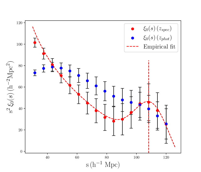
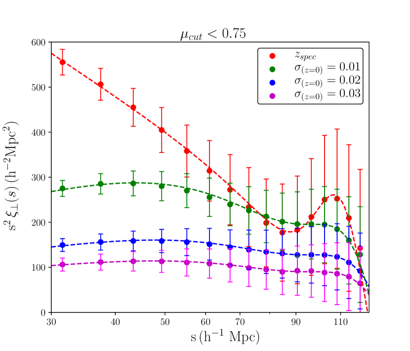
Figure 3: Left panel: The angle averaged monopole correlation function (multiplied by $s^{2}$) calculated for the spectroscopic sample (plotted in red) and for the $\sigma_{0}=0.01\,$photometric sample (plotted in blue) within the range $0.53<z<0.63$. The red dotted line shows the best-fit obtained from the empirical model in Eq. 8 for the spectroscopic sample. The vertical red dotted line shows the $s_{m}$ obtained from the best-fit to the spectroscopic sample. Right panel: The projected correlation function $\xi_{\perp}(s)\,$(multiplied by $s^{2}$) defined by Eq. 6 with $\mu_{\mathrm{cut}}<0.75$ for the spectroscopic sample (in red), the $\sigma_{0}=0.01\,$(in green), $\sigma_{0}=0.02\,$(in blue) and $\sigma_{0}=0.03\,$(in magenta) photometric samples. The dotted lines represent the best-fit model to the data obtained from Eq. 8. The error bars plotted in both the panels have been calculated using the full covariance matrix as mentioned in Eq. 9.

2.2 The BAO peaks imprinted on diverse correlation functions

The BAO feature is imprinted on the correlation function through the integrated effect of BAO signatures that remain in the power spectrum. We introduce all different configurations to describe the correlation function in redshift space, and discuss the optimised correlation function configuration to probe the BAO peaks from the photometric map. The correlation function $\xi$ is estimated using the Landy & Szalay estimator (hereafter LS) which is known to be less sensitive to the size of the random catalogue and also handles edge corrections better (Kerscher et al., 2000). The LS estimator in $(s,\mu)$ coordinates is given by,

$$\xi(s,\mu)=\frac{DD(s,\mu)-2DR(s,\mu)+RR(s,\mu)}{RR(s,\mu)},$$ (3)

where $DD$, $DR$ and $RR$ refer respectively to the number of data-data pairs, data-random pairs and the random-random pairs within a spherical shell of radius $s$ and $s+ds$ and the angle to the LOS $\mu$ and $\mu+d\mu$. The radius to shell $s$ and the observed cosine of the angle the pair makes with respect to the LOS $\mu$ are given by $s^{2}=\sigma^{2}+\pi^{2}$ and $\mu=\pi/s$ respectively, where $\sigma$ and $\pi$ denote the transverse and radial directions.

It is common practice to separate the random sample distributions into the angular and redshift components separately. For the angular components, we create random objects within the RA and DEC limits of the data catalogue. The number of objects are usually twice or more than the data catalogue to avoid shot noise effects. In our case the random catalogue has 5 times more objects than the data catalogue. For the redshift component, from the data catalogue we extract redshifts randomly within the chosen redshift range (see Ross et al., 2012; Veropalumbo et al., 2016, for more info). We use the publicly available KSTAT (KD-tree Statistics Package) code (Sabiu, 2018) to calculate all our correlation functions. A separate random catalogue is created for each realisation of the mocks because each realisation has it’s own distinct redshift distribution. We have verified that the difference between the correlation function calculated using the single spectroscopic random catalogue provided and the correlation function calculated using the distinct random catalogues is of the order of 3-5%.

In Fig.2, the anisotropy correlation function distorted in redshift space is presented in cartesian coordinates. The spectroscopic sample is given in the top-left panel along with the three different photometric samples in the other panels as denoted in the figure. We use a sinh${}^{-1}(300)\xi(\sigma,\pi)$ transform for the colour bar representation for easy visualisation as $\xi(\sigma,\pi)$ values extend from small to large values. The sinh${}^{-1}(x)$ function equals $x$ for $x\ll 1$ and ln $x$ for $x\gg 1$. BAO features are clearly observed at the outer contour encompassing $s\sim 110\,\mathrm{h}^{-1}\mathrm{Mpc}$ at both transverse and radial directions for the spectroscopy case, but are smeared out by the uncertainty of redshift measurement along the LOS for all the photometric cases. However, the errors propagate differently depending on the directions. It is not clearly visible if there are any remaining BAO features for the photometric cases. Thus we explore other diverse correlation configurations to extract the remaining BAO feature below.

When the objects have a spectroscopic redshift, it is useful to calculate the monopole correlation function $\xi_{0}(s)$, which is obtained by integrating $\xi(s,\mu)$ in $\mu$ direction,

$$\xi_{0}(s)=\int^{1}_{0}d\mu^{\prime}W(\mu^{\prime}:\mu_{\rm cut}=1)\xi(s,\mu^{\prime}),$$ (4)

where the weighting function $W(\mu^{\prime}:\mu_{\rm cut}=1)$ is given by $W(\mu^{\prime}:\mu=0$) at $\mu^{\prime}>\mu$, and it is normalised as,

$$\int^{1}_{0}d\mu^{\prime}W(\mu^{\prime}:\mu_{\rm cut})=1.$$ (5)

The cut–off $\mu$ is set to be $\mu_{\rm cut}=1$ for the monopole correlation function. In the left panel of Fig.3, BAO features observed from $\xi_{0}(s)$ using both the spectroscopic and photometric simulation maps are represented by red and blue points are respectively. While the peak is certainly visible around $s\sim 110\,\mathrm{h}^{-1}\mathrm{Mpc}$ in the spectroscopic map, it is smoothed out in the photometric map due to the uncertainty in the radial distance determination, with only the power law shape remaining at scales $s<80\,\mathrm{h}^{-1}\mathrm{Mpc}$ (Farrow et al., 2015; Sridhar et al., 2017)

As most contaminated pairs are found along the radial configuration, the correlation pairs at higher $\mu$ is trimmed out, and the cutoff $\mu$ is redefined in Eq. 4 as $\mu_{\rm cut}<1$. This incompletely integrated correlation function $\xi_{\perp}$ with the non–trivial $\mu_{\rm cut}$ will be an alternative option dubbed as the projected correlation function and is given by,

$$\xi_{\perp}(s)=\int^{1}_{0}d\mu^{\prime}W(\mu^{\prime}:\mu_{\rm cut}<1)\xi(s,\mu^{\prime})\,.$$ (6)

The reconstructed BAO features are obtained by trimming out the contaminated configuration along the LOS, in which a commonly used value of $\mu_{\rm cut}=0.75$ (Ross et al., 2017) is applied. The results are presented in the right panel of Fig. 3 for the spectroscopy and three photo-z uncertainty cases of $\sigma_{0}=(0.01,0.02,0.03)$. Although the observed BAO features from the photometric maps aren’t as clearly visible as the spectroscopy case, the shape of the correlation function is visibly improved using the projected correlation function.

The improvement by applying the projected correlation function suggests that the contaminated pairs can be removed by sorting the correlation function in $\mu$ bins. We pay attention to the usefulness of exploiting the wedge correlation function to separate the radial contamination from the BAO signal imprinted on perpendicular configuration pairs. The wedge correlation function $\xi_{w}$ is given by,

$$\xi_{w}(s,\mu_{i})=\int^{1}_{\mu_{i}^{\rm min}}d\mu^{\prime}W(\mu^{\prime}:\mu_{\rm cut}=\mu_{i}^{\rm max})\xi(s,\mu^{\prime}),$$ (7)

where $\mu_{i}$ is the mean $\mu$ in each bin, and $\mu_{i}^{\rm min}$ and $\mu_{i}^{\rm max}$ are the minimum and maximum values of $\mu$. We choose 6 bins in the $\mu$ direction with $\Delta\mu=0.17$ between $\mu=0$ and 1. The wedge correlation functions at $i=1,3,6$ are presented at the left, middle and right panels in Fig. 4. The $\xi_{w}$ with diverse photometric errors of $\sigma_{0}=(0,0.01,0.02,0.03)$ are shown from the top to the bottom panels. The BAO features are more contaminated at higher $i$.

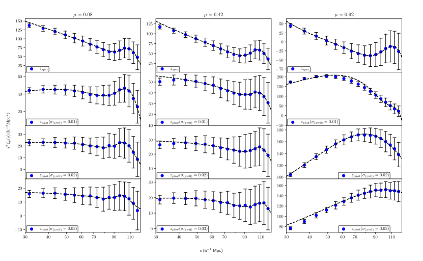
Figure 4: The correlation function $\xi(s,\mu)\,$(multiplied by $s^{2}$) calculated by splitting into wedges of $\mu$ given by the blue dots. The dashed black lines in each plot show the best-fit obtained from the empirical model in Eq. 8. The first, second and third columns in the figure represent $\bar{\mu}=0.08$, 0.42 and 0.92 bin respectively and the first, second, third and fourth rows in the figure represent the spectroscopic ($\sigma_{0}\approxeq 0$), $\sigma_{0}=0.01\,$, $\sigma_{0}=0.02\,$and $\sigma_{0}=0.03\,$photometric samples respectively. The error bars plotted have been calculated using the full covariance matrix as mentioned in Eq. 9.

2.3 Measurement of the residual BAO peaks

The empirical model that we use to fit the correlation function and obtain the BAO peak location is the one proposed by Sánchez et al. (2012), which is used to interpolate the correlation function at the BAO scales. It is given by:

$$\xi_{\rm mod}(s)=B+\left(\frac{s}{s_{0}}\right)^{-\gamma}+\frac{N}{\sqrt{2\pi\sigma^{2}}}\mathrm{exp}\left(-\frac{(s-s_{m})^{2}}{2\sigma^{2}}\right),$$ (8)

where $B$ takes into account a possible negative correlation at very large scales, $s_{0}$ is the correlation length (the scale at which the correlation function $\simeq$ 1) and $\gamma$ denotes the slope. These 3 parameters model the correlation function at small scales of $s<50\mathrm{h}^{-1}$Mpc, and are fixed firstly by fitting the data at scales below the BAO peak, i.e. $30<s\,(\mathrm{h}^{-1}\mathrm{Mpc})<80$. The remaining three parameters, $N$, $\sigma$ and $s_{m}$ are the parameters of the Gaussian function that model the BAO feature and, in particular, $s_{m}$ represents the estimate of the BAO peak position. This empirical model can be used to accurately predict the BAO peak position (Veropalumbo et al., 2016) when the correlation function is provided.

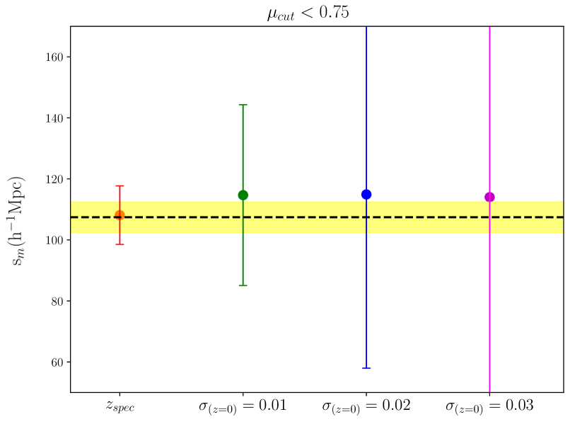
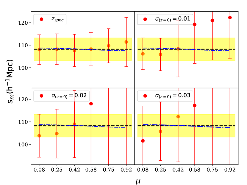
Figure 5: Left panel: The values of $s_{m}$ obtained from $\xi_{\perp}(s)\,$with $\mu_{cut}<0.75$. The x-axis denotes the spectroscopic, $\sigma_{0}=0.01\,$, $\sigma_{0}=0.02\,$and $\sigma_{0}=0.03\,$photometric samples as marked by the labels. The black dotted line in both the panels represents the value of $s_{m}$ obtained from the empirical fit for $\xi_{0}(s)$ calculated on the spectroscopic sample and the error on the same is given by the yellow highlighted region. Right panel: The x-axis denotes the 6 $\mu$ bins we have used and the y-axis denotes the value of $s_{m}$ obtained from the empirical fit for the spectroscopic sample (top left), $\sigma_{0}=0.01\,$(top right), $\sigma_{0}=0.02\,$(bottom left) and $\sigma_{0}=0.03\,$(bottom right) photometric samples. The blue dash-dotted line represents the $s_{m}$ obtained for the different $\mu$ bins from the theoretical template.

The means of the projected and wedge correlation functions are measured using 200 realisations. The covariance matrix of $\xi_{\perp}(s)$ and $\xi_{w}(s,\mu_{i})$ is computed as,

$$C^{ij}_{X}(\xi^{i}_{X},\xi^{j}_{X})=\frac{1}{N-1}\sum^{N}_{n=1}[\xi^{n}_{X}(\vec{x}_{i})-\overline{\xi}_{X}(\vec{x}_{i})][\xi^{n}_{X}(\vec{x}_{j})-\overline{\xi}_{X}(\vec{x}_{j})],$$ (9)

where $X$ denotes the symbols of $\perp$ or $w$ representing the projected or wedge correlation functions respectively, and the total number of $N$ is given by $N=200$. The $\xi^{n}_{X}(\vec{x}_{i})$ represents the value of the projected or wedge correlation function of $i^{th}$ bin of $\vec{x}_{i}$ in the $n^{th}$ realisation, and $\overline{\xi}_{X}(\vec{x}_{i})$ is the mean value of $\xi^{n}_{X}(\vec{x}_{i})$ over all the realisations. The number of realisations exceeds the number of $(s,\mu)$ bins of 96 bins, and the inverse of $C_{ij}$ is well defined and thus does not require any de-noising procedures such as singular value decomposition. Additionally, we also count the offset caused by the finite number of realisation as,

$$C^{-1}=\frac{N_{mocks}-N_{bins}-2}{N_{mocks}-1}\ \hat{C}^{-1}\ ,$$ (10)

where $N_{bins}$ denotes the total number of $i$ bins.

The fitting parameter space is given by $x_{p}=(B,s_{0},\gamma,N,s_{m},\sigma)$, and the BAO peak $s_{m}$ for the projected correlation function is estimated after fully marginalising all other parameters in $x_{p}$. The fitting function is given by,

$$\chi^{2}(x_{p})=\sum_{s,s^{\prime}}(\xi_{\rm mod}(s)-\xi_{\perp}(s))C^{-1}_{s;s^{\prime}}(\xi_{\rm mod}(s^{\prime})-\xi_{\perp}(s^{\prime}))$$ (11)

where $C^{-1}_{s;s^{\prime}}$ denotes the inverse covariance matrix for two different separation distances $s$ and $s^{\prime}$. For the wedge correlation function, the $\chi^{2}_{\mu_{i}}$ at each $\mu_{i}$ bin is expressed as,

$$\chi^{2}_{\mu_{i}}(x_{p})=\sum_{s,s^{\prime}}(\xi_{\rm mod}(s)-\xi_{w}(s,\mu_{i}))C^{-1}_{s;s^{\prime}}(\mu_{i})(\xi_{\rm mod}(s^{\prime})-\xi_{w}(s,\mu_{i}))$$ (12)

where $C^{-1}_{s;s^{\prime}}(\mu_{i})$ is the sub–inverse covariance matrix of $C^{-1}$ including the $\mu_{i}$ coordinate.

For $\xi_{\perp}$ with a non-trivial cut of $\mu_{\rm cut}<0.75$, Eq.8 is used to get $s_{m}$ for all the samples with varying $\sigma_{0}$. The $s_{m}$ values for all the samples are plotted in the left panel of Fig.5. For the spectroscopic sample, $s_{m}$ is measured with a fractional error of 8%, but the error propagation into the clustering by the photo-z uncertainty increases towards the radial direction. So, even though the $s_{m}$ obtained for the photo-z samples seem to be accurate within $1\sigma$ compared to the spectroscopic case, they are not precise, i.e. the errors are large. The error on $s_{m}$ increases with increasing $\sigma_{0}$.

Thus, to clearly examine the contamination of the pairs along the radial direction, it is necessary to split the correlation function into smaller $\mu$ bins and measure $\xi_{w}(s,\mu_{i})$. The $s_{m}$ values obtained from $\xi_{w}(s,\mu_{i})$ for the four $\sigma_{0}$ samples in the 6 $\mu$ bins used is shown in the right panel of Fig.5. As a benchmark, we make use of the $s_{m}$ obtained from $\xi_{0}(s)$ using the spectroscopic sample (black dotted line, with $1\sigma$ error given by the yellow highlighted region) along with the $s_{m}$ obtained from the theoretical template (explained in Section 3.1 and given by the blue dot-dashed line). For all $\bar{\mu}<0.42$, it can be seen that the $s_{m}$ obtained is within $1\sigma$ compared to the $s_{m}$ from $\xi_{0}(s)$. On the other hand, for all $\bar{\mu}>0.42$, only the $s_{m}$ from the spectroscopic sample seems to be within $1\sigma$. This strongly suggests that measuring the BAO peak within $\bar{\mu}<0.42$ gives us tight constraints even when we have photometric samples with an error of $\sigma_{0}=0.03\,$.

3 The measured cosmic distances using photometric samples

The volume distance $D_{V}(z)=\left[(1+z)^{2}D_{A}(z)^{2}cz/H(z)\right]^{1/3}$ is measured through the BAO by exploiting the monopole correlation function. While the monopole correlation function is preferably used without any concerns regarding the computation of the covariance matrix, both the transverse and radial cosmic distances can be separately measured using the 2D anisotropy correlation function. The full covariance matrix determination for the 2D anisotropy correlation function is much more difficult, but the estimated covariance matrix appears to be stable, at least numerically with the number of realisations we have used for the simulations. When both the transverse and radial distance measures of redshift are precisely probed, both $D_{A}$ and $H^{-1}$ are determined with high precision. In case there exists a systematic uncertainty in determining the radial component, the methodology of using the 2D anisotropy correlation function can be useful to remove the contaminated cosmological information along the LOS. In this section, we verify whether the transverse cosmic distance can be measured in precision regardless of the photo-z uncertainty.

3.1 Theoretical model to fit cosmic distances

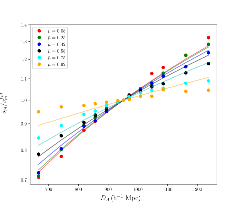
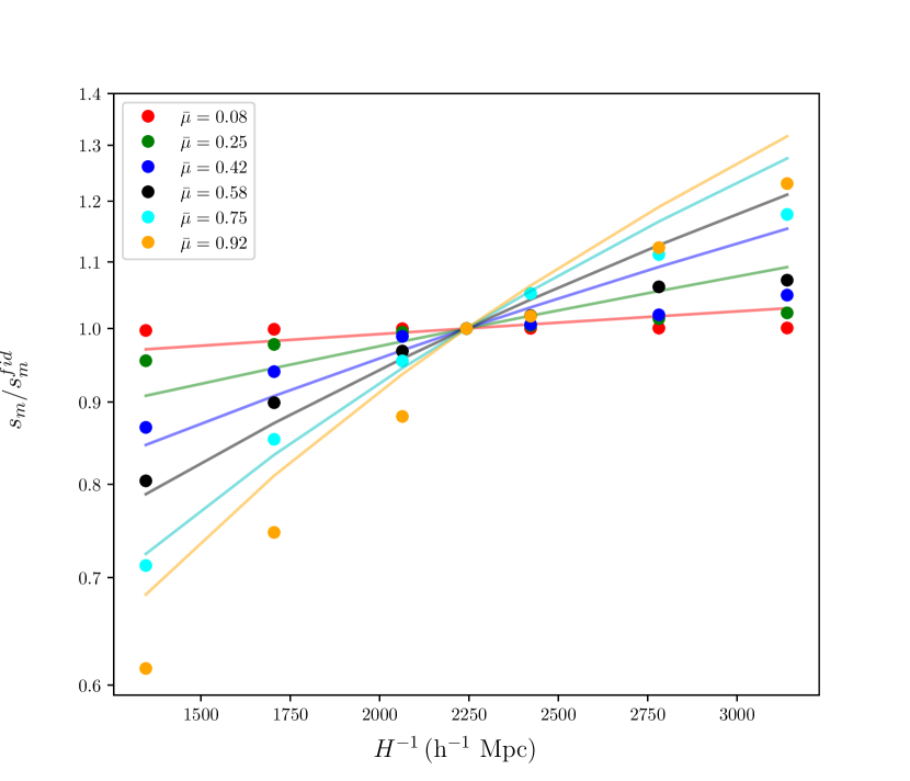
Figure 6: Left panel: The values of $s_{m}/s_{m}^{fid}$ for the 6 $\mu$ bins at different values of $D_{A}$ computed using the TNS model given by the dotted points as colour coded. The solid curves represent the same obtained using a simple coordinate projection from the fiducial value. Right panel: The same as the left panel, but for different values of $H^{-1}$. Units are in $\rm\mathrm{h}^{-1}\rm Mpc$.

We need to theoretically model the correlation function to fit the cosmological distance variations. The theoretical correlation function in redshift space $\xi_{\rm th}(s,\mu)$ is computed using the improved power spectrum in the perturbative expansion as,

$$\xi_{\rm th}(s,\mu) = \int\frac{d^{3}k}{(2\pi)^{3}}\tilde{P}(k,\mu^{\prime})e^{i{\bf k}\cdot{\bf s}}$$ (13)

$$= \sum_{\ell:{\rm even}}\xi_{\ell}(s){\cal P}_{\ell}(\mu)\,,$$

with ${\cal P}$ being the Legendre polynomials. Here, we define $\nu=\pi/s$ and $s=(\sigma^{2}+\pi^{2})^{1/2}$. The moments of the correlation function, $\xi_{\ell}(s)$, are defined by,

$$\xi_{\ell}(s)=i^{\ell}\int\frac{k^{2}dk}{2\pi^{2}}\,\tilde{P}_{\ell}(k)\,j_{\ell}(ks)\,.$$ (14)

The multipole power spectra $\tilde{P}_{\ell}(k)$ are explicitly given by,

$$\tilde{P}_{0}(k) = p_{0}(k),$$

$$\tilde{P}_{2}(k) = \frac{5}{2}\left[3p_{1}(k)-p_{0}(k)\right],$$

$$\tilde{P}_{4}(k) = \frac{9}{8}\left[35p_{2}(k)-30p_{1}(k)+3p_{0}(k)\right],$$

where we define the function $p_{m}(k)$:

$$p_{m}(k) = \frac{1}{2}\sum_{n=0}^{4}\frac{\gamma(m+n+1/2,\kappa)}{\kappa^{m+n+1/2}}\,Q_{2n}(k)$$ (16)

with $\kappa=k^{2}\sigma_{p}^{2}$. The function $\gamma$ is the incomplete gamma function of the first kind:

$$\gamma(n,\kappa)=\int^{\kappa}_{0}dt\,t^{n-1}\,e^{-t}\,.$$ (17)

The $Q_{2n}$ is explained below.

The observed power spectrum in redshift space $\tilde{P}(k,\mu)$ is written in the following form;

$$\tilde{P}(k,\mu)=\sum_{n=0}^{8}\,Q_{2n}(k)\mu^{2n}\,G^{\rm FoG}(k\mu\sigma_{p})\,,$$ (18)

where the velocity dispersion $\sigma_{p}$ is set to be a free parameter for FoG effect, and the function $Q_{2n}$ are given by,

$$Q_{0}(k) = P_{\delta\delta}(k),$$

$$Q_{2}(k) = 2P_{\delta\Theta}(k)+C_{2}(k),$$

$$Q_{4}(k) = P_{\Theta\Theta}(k)+C_{4}(k),$$ (19)

where $C_{n}$ includes the nonlinear correction terms $A$ and $B$, and $P_{XY}(k)$ denotes the power spectrum in real space. The standard perturbation model exhibits the ill-behaved expansion leading to the bad UV behaviour which is regularised by introducing UV cut-off in this manuscript. The treatment of resummed perturbation theory dubbed as RegPT is well explained in Taruya et al. (2012). The auto and cross spectra of $P_{XY}(k)$ are computed up to first order, and higher order polynomials $A$ and $B$ are computed up to zeroth order, which are consistent in the perturbative order.

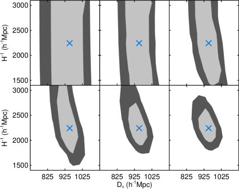
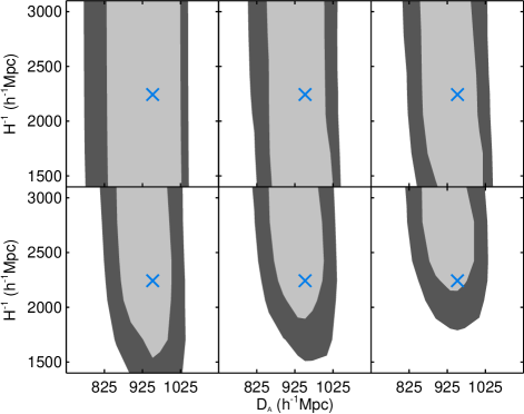
Figure 7: Left panel: Constraints at the 68 and 95 per cent confidence limit on the parameters $D_{A}$ and $H^{-1}$ obtained from the spectroscopic sample. The $\chi^{2}_{m}$ values used are from $\bar{\mu}=0.08$ (top left), $\bar{\mu}=0.08+0.25$ (top middle), $\bar{\mu}=0.08+0.25+0.42$ (top right), $\bar{\mu}=0.08+0.25+0.42+0.58$ (bottom left), $\bar{\mu}=0.08+0.25+0.42+0.58+0.75$ (bottom middle) and $\bar{\mu}=0.08+0.25+0.42+0.58+0.75+0.92$ (bottom right). The blue cross marks the fiducial value of $D_{A}$ and $H^{-1}$. Units are in $\mathrm{h}^{-1}\mathrm{Mpc}$. Right panel: The constraints obtained from the $\sigma_{0}=0.01\,$photometric sample with the same methodology of adding up the $\chi^{2}_{m}$ values.

There are challenges in computing the theoretical prediction of galaxy clustering in redshift space. Although cosmic distances are estimated using the BAO at linear regimes, the small peak structure tends to be smeared out by non–linear physics which needs to be computed. In addition, the infinite higher order polynomials are generated due to the density and velocity correlations. Those perturbative corrections in a more elaborate description are included to make precise prediction of the BAO structure (Taruya et al., 2010). Finally, those perturbative effects and non–linear smearing effects on the clustering are not separately modelled. Taking account of this fact, Taruya et al. (2010) proposed an improved model of the redshift-space power spectrum, in which the coupling between the density and velocity fields associated with the Kaiser and the FoG effects is perturbatively incorporated into the power spectrum expression. The resultant includes nonlinear corrections consisting of higher-order polynomials (Taruya et al., 2010):

$$\tilde{P}(k,\mu) = \big{\{}P_{\delta\delta}(k)+2\mu^{2}P_{\delta\Theta}(k)+\mu^{4}P_{\Theta\Theta}(k)$$ (20)

$$+ A(k,\mu)+B(k,\mu)\big{\}}G^{\rm FoG}$$

Here the $A(k,\mu)$ and $B(k,\mu)$ terms are the nonlinear corrections, and are expanded as power series of $\mu$. Those spectra are computed using the fiducial cosmological parameters. The FoG effect $G^{\rm FoG}$ is given by the simple Gaussian function which is written as,

$$G^{\rm FoG}\equiv\exp{\left[-(k\mu\sigma_{p})^{2}\right]}$$ (21)

where $\sigma_{p}$ denotes one dimensional velocity dispersion. Thus the theoretical correlation function $\xi_{th}$ is parameterised by ($D_{A},H^{-1},G_{b},G_{\Theta},\sigma_{p}$) wherein $G_{b}$ and $G_{\Theta}$ are the normalised density and coherent motion growth functions. The BAO feature is weakly dependent on the growth functions and $\sigma_{p}$. When working with spectroscopic redshift samples for which the error on the redshift is negligible, we can marginalise over the above set of 5 parameters and the corresponding $\xi_{th}(s,\mu)$ can be used as the fit to the observed $\xi(s,\mu)\,$. But when working with photo-z samples, the effect of the photo-z error on the correlation function is incoherent. Thus, the extra parameter needed for the theoretical template to model $\xi_{th}(s,\mu)$ as a function of the photo-z error is not well understood. So, we use Eq. 8 instead to fit our observed $\xi(s,\mu)\,$. This functional form only assumes a power-law at small scales and a Gaussian function to fit the BAO peak at large scales and seems to model $\xi(s,\mu)\,$quite well as we can see from Fig. 4. The effect of the photo-z error on $\xi_{th}(s,\mu)$ and its marginalisation is kept for future work.

In this verification work, when we fit the cosmic distances, we vary the tangential and radial distance measures from the fiducial values of $D_{A}=951.80\,\mathrm{h}^{-1}\mathrm{Mpc}$ and $H^{-1}=2243.04\,\mathrm{h}^{-1}\mathrm{Mpc}$. The best fit $\sigma_{p}$ for this simulation is found to be $\sigma_{p}=4.2\,\mathrm{h}^{-1}\mathrm{Mpc}$. Note that we apply the TNS model for computing the theoretical BAO peaks to fit the measured data. The theoretical BAO peaks at the fiducial cosmology can be transformed into a new cosmology according to the simple coordinate projections, which are presented as solid curves in Fig. 6. But the location shift of BAO peak with varying $D_{A}$ and $H^{-1}$ is not completely consistent with coordinate transformation. The theoretical BAO peaks computed using the TNS model are represented by dotted points. The difference is exceeding the dectectability limit by about 5%, and thus the TNS model is adopted to determine the theoretical BAO points.

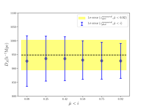
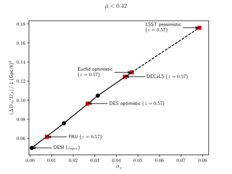
Figure 8: Left panel: The measured $D_{A}$ and the corresponding $1\sigma$ errors calculated using $\chi^{2}_{m}(\bar{\mu}<i)$, where $i$ goes from 0.08 to 0.92, for the $\sigma_{0}=0.01$ photometric sample (plotted using the blue dots). The dashed black line denotes the measured $D_{A}$ using $\chi^{2}_{m}(\bar{\mu}<0.92)$ for the spectroscopic sample along with the yellow highlighted region denoting the $1\sigma$ errors. Right panel: $\sigma_{z}$ vs $\Delta D_{A}/D_{A}$ per 1 (Gpc$/h)^{3}$ for $\bar{\mu}<0.42$. All the values of $\sigma_{z}$ correspond to the median redshift $\bar{z}=0.57$. The three black dots are values obtained for the spectroscopic redshift, $\sigma_{0}=0.01$ and 0.02 respectively. The red squares give us values of $\Delta D_{A}/D_{A}$ for different surveys based on their expected $\sigma_{0}$. The dotted black line is a crude approximation out to $\sigma_{0}=0.05$ corresponding to the LSST pessimistic case.

3.2 Measured cosmic distances

With the given fiducial cosmology, both the tangential and radial BAO peak locations can be computed by varying $D_{A}(z)$ and $H^{-1}(z)$ using the theoretical templates introduced in the previous subsection. The cosmic distances estimated from the measured BAO peak locations at all 6 $\mu$ bins are shown in Fig.7. Different combinations of $\mu_{i}$ bins in which all bins of $\mu_{i}$ with $i<i_{\rm max}$ are cumulatively summed and the $i_{\rm max}$ runs from 1 at the top left to 6 at the bottom right.

In principle, because the BAO ring spans both the transverse and radial cosmological coordinates, it can be exploited to probe the distance measures of $D_{A}(z)$ and $H^{-1}(z)$ separately. If there is minimal photo-z uncertainty, then both cosmic distances are precisely measured as presented in the left panel of Fig.7. The uncertainty on the redshift determination prevents us from accessing the radial cosmic distance, and thus $H^{-1}(z)$ is poorly determined as presented in the right panel. However, note that the transverse distance is measured precisely regardless of the systematic uncertainty along the radial direction. Although $D_{A}(z)$ is measured after full marginalisation over $H^{-1}(z)$, the precision loss in the $D_{A}(z)$ measurement is negligible, which can be compared between the left and right panels of Fig.7. The constraints obtained on the fiducial and the measured $D_{A}(\bar{z}=0.57)$ from the photometric sample when $i<(i_{\rm max}=6)$ are $D_{A}(\bar{z}=0.57)=951.80^{+37.40}_{-87.80}\,\mathrm{h}^{-1}\mathrm{Mpc}$ and $D_{A}(\bar{z}=0.57)=927.00^{+63.00}_{-63.01}\,\mathrm{h}^{-1}\mathrm{Mpc}$ respectively. The constraints on $D_{A}(z)$ and $H^{-1}(z)$ improve with increasing $i_{\rm max}$. The error on $D_{A}(z)$ decreases from 9.5% (for $i_{\rm max}=1$) to 5.7% (for $i_{\rm max}=6)$ for the spectroscopic sample and a similar trend is observed for the $\sigma_{0}=0.01\,$photometric sample, with the error on $D_{A}(z)$ decreasing from 9.8% to 6.5% as shown in the left panel of Fig.8.

The constraints obtained on $D_{A}(z)$ not only depend on $\sigma_{0}$ and $z$, but also on the volume covered by the survey. In the right panel of Fig.8 we plot $\sigma_{z}$ vs $\Delta D_{A}/D_{A}$ per 1 (Gpc$/h)^{3}$ at $\bar{z}=0.57$ and $\bar{\mu}<0.42$ for the spectroscopic and the two ($\sigma_{0}=0.01,0.02$) photometric cases which are denoted by the black dots. We also plot the $\Delta D_{A}/D_{A}$ for different surveys (red squares) based on their expected $\sigma_{0}$, starting with 0.005 for the PAUS survey (Benítez et al., 2009; Martí et al., 2014), 0.017 for DES Y1 high luminosity ‘redmagic’ (Rozo et al., 2016) sample, 0.028 (Zhou. et al 2019, in preparation) for DECaLS (Dey et al., 2018) LRGs and 0.030 for Euclid (Laureijs et al., 2011). The black dotted line is a crude approximation out to $\sigma_{0}=0.05$ which corresponds to the LSST pessimistic case (Ivezic et al., 2008; LSST Science Collaboration et al., 2009).

4 Discussion and conclusions

We study the statistical methodology to extract the cosmic distance information from photometric galaxy samples, using the simulated photometric galaxy distribution based on the DR12 CMASS map. The measured monopole moment of the two-point correlation function is so significantly contaminated by the uncertainty in redshift determination that the BAO feature is smeared out completely. The common practice to extract the BAO peak is to exploit the incomplete angular averaged correlation which is known as the projected correlation function. When the most contaminated correlation configuration along the LOS is removed, the BAO peak starts becoming visible.

In this manuscript, the wedge is binned into 6 pieces using equal $\mu$ spacing from $\mu=0$ to 1 and we analyse each wedge component one by one and present the level of contamination due to the $z$ uncertainty, in comparison to the spectroscopic map. We find that the first two wedge correlations are least contaminated by the $z$ uncertainty. The noticeable contamination is observed from the third $\mu$ bin with the BAO peak still visible. The transverse cosmic distance is probed with a reasonably good precision as presented in Fig.8. Those wedges are coherently summed using the full covariance matrix, and the cumulative constraint on $D_{A}$ is presented to show the information is nearly saturated at the first several bins. For the radial component of the cosmic distance, we are not able to extract it from the photometric sample, as most radial information is contained at wedge bins higher than $\mu_{i}$ with $i\ga 4$, which is contaminated by the $z$ uncertainty. However, the measured transverse cosmic distance is immune from this uncertainty. The reported values of $D_{A}$ in Fig.8 is computed after full marginalisation of $H^{-1}$. The measured $D_{A}$ is not biased by this marginalisation.

Multiband imaging surveys rely on photometric redshift for radial information. The Dark Energy Survey (DES) (The Dark Energy Survey Collaboration, 2005) and future surveys such as LSST (Ivezic et al., 2008; LSST Science Collaboration et al., 2009) and Euclid (Laureijs et al., 2011) will provide state-of-the-art photometric redshifts over an unprecedented range of redshift scales. The precision that is expected from the photometric redshifts is typically 3% (Rozo et al., 2016). Some of the recent works that have used photometric redshift catalogues have focused on measuring the angular correlation function $w(\theta)$ to get cosmic distance measurements (Sánchez et al., 2011; Seo et al., 2012; Carnero et al., 2012) using several narrow redshift slices. However, they clearly do not use the full information available, as radial binning blends data beyond what is induced by the photometric redshift error. Another important aspect that is often ignored when calculating $w(\theta)$ is cross correlation between the different redshift bins used. Using many redshift slices also complicates the computation of the covariance matrix, with the computing time increasing with the number of bins in $\theta$ and number of redshift slices used. It has also been shown recently by Ross et al. (2017) that the statistics obtained using $\xi(s,\mu)\,$are about 6% more accurate compared to $w(\theta)$. Thus, using $\xi(s,\mu)\,$not only adds more information compared to $w(\theta)$, but also overcomes the above disadvantages.

The full photometric footprints for DESI were released ahead of the spectroscopic follow up. We have shown here that the transverse component of cosmic distance can be pre–measured using the photometric galaxy map even without the need of a spectroscopic follow up in the future. In addition, the photometric survey leads us to deeper redshifts which will not be probed by the spectroscopic survey. For instance, the spectroscopic LRG sample ends at redshift $z\sim 0.8$, but the photometric sample reaches up to $z\ga 1.0$. We verify in this manuscript that we are able to probe the transverse distance at a higher redshift using the photometric map. In our next project, this verified method will be applied to measure cosmic distances for the DECaLS (Dey et al., 2018) DR7 photometric LRG galaxy map (Zhou. et al 2019, in preparation) at redshift ranges of $0.6<z_{phot}<0.8$ and $0.8<z_{phot}<1.0$. The spectroscopic follow up survey fully covers LRG galaxies in the range of $0.6<z<0.8$, and partially for the $0.8<z<1.0$ case. If the cosmic distance at $0.8<z<1.0$ is successfully measured, then we will be able to probe cosmological information that is not fully covered by the spectroscopic survey.

References

- Alam et al. (2017) Alam S., et al., 2017, MNRAS, 470, 2617
- Ascaso et al. (2015) Ascaso B., Mei S., Benítez N., 2015, MNRAS, 453, 2515
- Benedict et al. (1999) Benedict G. F., et al., 1999, AJ, 118, 1086
- Benítez et al. (2009) Benítez N., et al., 2009, ApJ, 691, 241
- Benitez et al. (2014) Benitez N., et al., 2014, arXiv e-prints, p. arXiv:1403.5237
- Blake & Glazebrook (2003) Blake C., Glazebrook K., 2003, ApJ, 594, 665
- Carnero et al. (2012) Carnero A., Sánchez E., Crocce M., Cabré A., Gaztañaga E., 2012, MNRAS, 419, 1689
- DESI Collaboration et al. (2016) DESI Collaboration et al., 2016, arXiv e-prints, p. arXiv:1611.00036
- Davis & Peebles (1983) Davis M., Peebles P. J. E., 1983, ApJ, 267, 465
- Dey et al. (2018) Dey A., et al., 2018, preprint, (arXiv:1804.08657)
- Eisenstein et al. (1998) Eisenstein D. J., Hu W., Tegmark M., 1998, ApJ, 504, L57
- Eisenstein et al. (2005) Eisenstein D. J., et al., 2005, ApJ, 633, 560
- Estrada et al. (2009) Estrada J., Sefusatti E., Frieman J. A., 2009, ApJ, 692, 265
- Farrow et al. (2015) Farrow D. J., et al., 2015, MNRAS, 454, 2120
- Fernie (1969) Fernie J. D., 1969, PASP, 81, 707
- Hong et al. (2012) Hong T., Han J. L., Wen Z. L., Sun L., Zhan H., 2012, ApJ, 749, 81
- Howlett et al. (2012) Howlett C., Lewis A., Hall A., Challinor A., 2012, JCAP, 1204, 027
- Ivezic et al. (2008) Ivezic Z., et al., 2008, preprint, (arXiv:0805.2366)
- Kazin et al. (2013) Kazin E. A., et al., 2013, MNRAS, 435, 64
- Kerscher et al. (2000) Kerscher M., Szapudi I., Szalay A. S., 2000, ApJ, 535, 13
- LSST Science Collaboration et al. (2009) LSST Science Collaboration et al., 2009, preprint, (arXiv:0912.0201)
- Laureijs et al. (2011) Laureijs R., et al., 2011, preprint, (arXiv:1110.3193)
- Lewis et al. (2000) Lewis A., Challinor A., Lasenby A., 2000, Astrophys. J., 538, 473
- Manera et al. (2013) Manera M., et al., 2013, MNRAS, 428, 1036
- Martí et al. (2014) Martí P., Miquel R., Castander F. J., Gaztañaga E., Eriksen M., Sánchez C., 2014, MNRAS, 442, 92
- Padilla et al. (2019) Padilla C., et al., 2019, arXiv e-prints, p. arXiv:1902.03623
- Padmanabhan et al. (2012) Padmanabhan N., Xu X., Eisenstein D. J., Scalzo R., Cuesta A. J., Mehta K. T., Kazin E., 2012, MNRAS, 427, 2132
- Peebles & Yu (1970) Peebles P. J. E., Yu J. T., 1970, ApJ, 162, 815
- Perlmutter et al. (1999) Perlmutter S., et al., 1999, ApJ, 517, 565
- Riess et al. (1998) Riess A. G., et al., 1998, AJ, 116, 1009
- Ross et al. (2012) Ross A. J., et al., 2012, MNRAS, 424, 564
- Ross et al. (2017) Ross A. J., et al., 2017, MNRAS, 472, 4456
- Rozo et al. (2016) Rozo E., et al., 2016, MNRAS, 461, 1431
- Sabiu (2018) Sabiu C., 2018, KSTAT: KD-tree Statistics Package, Astrophysics Source Code Library (ascl:1804.026)
- Sabiu & Song (2016) Sabiu C. G., Song Y.-S., 2016, preprint, (arXiv:1603.02389)
- Sánchez et al. (2011) Sánchez E., et al., 2011, MNRAS, 411, 277
- Sánchez et al. (2012) Sánchez A. G., et al., 2012, MNRAS, 425, 415
- Sánchez et al. (2014a) Sánchez A. G., et al., 2014a, MNRAS, 440, 2692
- Sánchez et al. (2014b) Sánchez C., et al., 2014b, MNRAS, 445, 1482
- Sánchez et al. (2017) Sánchez A. G., et al., 2017, MNRAS, 464, 1640
- Seo et al. (2012) Seo H.-J., et al., 2012, ApJ, 761, 13
- Sridhar et al. (2017) Sridhar S., Maurogordato S., Benoist C., Cappi A., Marulli F., 2017, A&A, 600, A32
- Taruya et al. (2010) Taruya A., Nishimichi T., Saito S., 2010, Phys. Rev. D, 82, 063522
- Taruya et al. (2012) Taruya A., Bernardeau F., Nishimichi T., Codis S., 2012, Phys. Rev. D, 86, 103528
- Taylor (2005) Taylor M. B., 2005, in Shopbell P., Britton M., Ebert R., eds, Astronomical Society of the Pacific Conference Series Vol. 347, Astronomical Data Analysis Software and Systems XIV. p. 29
- The Dark Energy Survey Collaboration (2005) The Dark Energy Survey Collaboration 2005, ArXiv Astrophysics e-prints,
- Totsuji & Kihara (1969) Totsuji H., Kihara T., 1969, PASJ, 21, 221
- Veropalumbo et al. (2014) Veropalumbo A., Marulli F., Moscardini L., Moresco M., Cimatti A., 2014, MNRAS, 442, 3275
- Veropalumbo et al. (2016) Veropalumbo A., Marulli F., Moscardini L., Moresco M., Cimatti A., 2016, MNRAS, 458, 1909