Stockholm University, AlbaNova University Centre, SE-106 91 Stockholm
On the ratio of lapses in bimetric relativity
Abstract
The two lapse functions in the Hassan–Rosen bimetric theory are not independent. Without knowing the relation between them, one cannot evolve the equations in the 3+1 formalism. This work computes the ratio of lapses for the spherically symmetric case, which is a prerequisite for numerical bimetric relativity.
Keywords:
Modified gravity, Bimetric relativity, Ghost-free bimetric theory1 Introduction
This work establishes the relationship between the two lapse functions in the Hassan-Rosen (HR) bimetric theory when the equations are reduced to the spherically symmetric case. The HR theory Hassan:2011zd ; Hassan:2011ea ; Hassan:2017ugh ; Hassan:2018mbl is a nonlinear theory of two interacting classical spin-2 fields. It is closely related to de Rham–Gabadadze–Tolley (dRGT) massive gravity, where one of the metrics is frozen and taken to be a nondynamical fiducial metric deRham:2010ik ; deRham:2010kj ; Hassan:2011hr . Comprehensive reviews of these theories can be found in Schmidt-May:2015vnx ; deRham:2014zqa .
As shown in Hassan:2018mbl ; Alexandrov:2012yv , the ratio of the two lapses in the HR theory is a function of the dynamical variables only. Without exactly knowing their relation in 3+1 formalism, one cannot set up the initial value problem and evolve the equations of motion in numerical bimetric relativity. Here we evaluate the ratio of the lapses for the case of spherical symmetry. The calculation is based on the evolution equations in standard 3+1 form Kocic:2018ddp .
Background
Similarly to general relativity Arnowitt:1962hi ; York:1979aa , the kinematical and dynamical parts of the metric fields in bimetric relativity can be isolated using the 3+1 formalism. However, there are two seemingly different paths in attacking the problem. One approach begins with the 3+1 split at the level of the action. This path is suitable for the Hamiltonian formulation and the canonical analysis of constraints Hassan:2018mbl . The other approach starts from the 3+1 projection of the field equations Kocic:2018ddp . This is more in line with the initial value formulation of the theory. The comparison of these two approaches is shown in Figure 1.
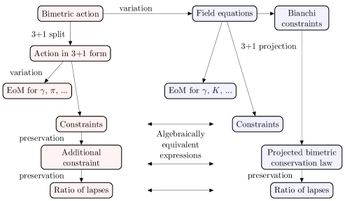
These procedures should and do yield equivalent results. The canonical analysis provides a fundamental view on the structure and the relation between the constraints. On the other hand, a direct 3+1 projection of the field equations is less involved (i.e., faster), and more suitable as the starting point towards numerical bimetric relativity. In the rest of the paper we traverse both paths in Figure 1. More specifically, the canonical analysis is used to prove that the ratio of lapses only depends on the dynamical fields in the most general case. The actual calculations in spherical symmetry will be based on the HR field equations in standard 3+1 form.
The rest of this paper is structured as follows. We begin by stating the action, the field equations, and the 3+1 decomposition of both the metrics and the square root in the potential. We then investigate the relationship between the lapses using the constraint analysis, and quote the basic equations that are used as a starting point. Subsection 2.2 states the bimetric conservation law (the so-called secondary constraint) for the case of spherical symmetry, and establishes the evolution equation for the relative shift between the two metrics, called the ‘separation parameter’. Subsection 2.3 presents the actual derivation of the ratio of lapses. The paper ends with a short discussion of the result.
Action.
The Hassan-Rosen action reads Hassan:2011zd ,
| (1) |
where and are the Ricci scalars of and , respectively, and are the Einstein gravitational constants for the two sectors, and are free parameters which are dimensionless and scaled by . The respective Lagrangian densities of the two matter sectors are denoted as and . The ghost-free bimetric interactions are specifically constructed using the elementary symmetric polynomials in terms of the principal square root matrix that represents a (1,1) tensor field Hassan:2017ugh .
Field equations.
The bimetric field equations can be written,
| (2) |
where and are the Einstein tensors of and , and are the stress–energy tensors of the matter fields each minimally coupled to a different sector, and and are the stress–energy contributions of the ghost-free bimetric potential, also known as the bimetric stress–energy tensors.
The 3+1 decomposition.
We assume that the metrics are in the usual 3+1 form,
| (3a) | ||||
| (3b) | ||||
where and are the spatial metrics, and are the shift vectors, and and are the lapse functions.
The square root.
The ghost-free bimetric interactions are specifically constructed in terms of the square root matrix . The chief condition is the existence and uniqueness of the real square root Hassan:2017ugh . Upon 3+1 decomposition, the condition can be expressed in terms of the affine related variables and via the mean shift vector ,
| (4) |
These variables are connected through , or in matrix notation,
| (5) |
where is defined in Hassan:2011tf , and are the symmetrized spatial vielbeins of and , while is the boost vector of the Lorentz transformation that is used to symmetrize the vielbeins ensuring the reality of the square root Hassan:2014gta ; Kocic:2018ddp . Geometrically, these shift-like vectors encode the separation (a relative shift) between the two metrics, which can equally be parametrized by . In other words, the variables , , and are “three” sides of the same coin. Note that does not depend on the two lapse functions, and that because of the overall local Lorentz invariance that was used to symmetrize the vielbeins.
1.1 Canonical analysis of the constraints
In the following two subsections we briefly summarize the constraint analysis of Hassan:2018mbl . In order to isolate the constraints, we need to eliminate one of the shift vectors, for instance , in terms of one of the new variables, for example , using (4),
| (6) |
Note that this choice is arbitrary. For this particular choice, the Lagrangian is linear in , and , and can be written,
| (7) |
where and denote the canonical momenta of and , respectively. The quantities , , and are defined in (39) and (40). Variation with respect to the lapse functions and the shift vector gives rise to the constraints,
| (8) |
These equations depend on and varying the Lagrangian with respect to yields its equations of motion,
| (9) |
where is defined in (39c). Equation (9) can in principle be solved for in terms of the dynamical variables. After imposing that solution on (8), those equations depend only on the dynamical variables.
Since the constraints are valid at all times, their time derivatives must vanish on the constraint surface. This can be used to find an additional constraint. The time derivative of a quantity is determined by its Poisson bracket with the Hamiltonian,
| (10) |
From this we see that the time derivatives of the constraints involve Poisson brackets of the constraints with each other. These brackets are computed in Hassan:2018mbl and read,
| (11) | ||||
| (12) | ||||
| (13) | ||||
| (14) | ||||
| (15) | ||||
| (16) |
Here, the expression for is a function of the phase space variables defined in (42). Note that all of the brackets, except for (16), vanish upon imposing the constraints (8). Therefore, it follows that,
| (17) |
where the symbol denotes weak equality, that is, equality on the constraint surface. Since and are nonzero and all expressions in (17) vanish on the constraint surface, this means that we must have,
| (18) |
which provides us with an additional constraint.
1.2 Ratio of lapses in the canonical analysis
Since the constraint (18) must be valid at all times, it is necessary that , where now denotes equality on the surface of all six constraints (8) and (18). Here we show that the requirement gives a linear relation between the two lapses for the most general case. The time derivative is given by,
| (19) |
We now consider each of the Poisson brackets that appear in this expression. In order to compute them we use,
| (20) |
which follows from (16). We also use the Jacobi identity, . The final Poisson bracket in (19) can then be written,
| (21) |
where (12), (14), and (16) have been used (see appendix A for the details). Note that this means that this bracket vanishes on the constraint surface.
We turn our attention to the second bracket in (19). It can be written,
| (22) |
From (13) and (14), it follows that the second term vanishes; hence,
| (23) |
where we have used (16). We see that this bracket is symmetric with respect to interchange of and . The first bracket in (19) can be dealt with in a similar way,
| (24) |
It follows from (15) and (16) that the first term vanishes weakly, implying,
| (25) | ||||
| (26) |
To summarize, we have,
| (27) | ||||
| (28) |
In order to compute these brackets, define the smeared constraints,
| (29) |
where and are arbitrary localized smoothing functions. It follows that,
| (30) |
which means that if we compute , we can extract . The most general expression for is Alexandrov:2012yv ,
| (31) |
where , and are some functions of the phase space variables. From (27) it follows that this expression should be symmetric with respect to interchanges of and . In order for this to be the case, we must have . Consequently,
| (32) |
where in the second step we use integration by parts. Here we have defined . Hence, we obtain,
| (33) |
We can use identical reasoning when computing . Using (28) we get,
| (34) |
The functions and depend on the phase space variables. We can now plug the expressions (21), (33) and (34) into (19) to arrive at,
| (35) |
Note that the terms involving the shift vanish weakly, being proportional to or its spatial derivative. As mentioned, , which implies,
| (36) |
This yields the ratio of lapses,
| (37) |
In conclusion, the requirement gives a linear relation between the two lapses.
1.3 Bimetric field equations in standard 3+1 form
Here we highlight the second approach in Figure 1, where the evolution and the constraint equations are obtained by projection of the bimetric field equations. After the projection, the standard 3+1 evolution equations are Kocic:2018ddp ,
| (38a) | |||||
| (38b) | |||||
| (38c) | |||||
| (38d) | |||||
where denotes a Lie derivative, and are the extrinsic curvatures in the two sectors, and are the spatial Ricci tensors, and and are the spatial covariant derivatives compatible with and , respectively.111Note that and . The indices are raised/lowered by the metric in the respective sector. The variables and denote the normal, tangential and spatial projections of the effective stress–energy tensors in the two sectors, which include both the contributions from matter and the bimetric potential. These can be split into the bimetric contribution denoted by upper label “b” and the matter contribution denoted by upper label “m”, for instance, .
The constraint equations are,
| (39a) | ||||||||
| (39b) | ||||||||
| (39c) | ||||||||
| (39d) | ||||||||
Note that the constraints for the mixed projections (39c)–(39d) are algebraically coupled by , which yields,
| (40) |
where and are the tangential projections of the matter stress–energy tensors only. The last equation can be used as a replacement for either (39c) or (39d), where the other becomes the equation of motion for (or or ). The contributions of the bimetric stress–energy tensors can be expressed in terms of the following set of 3+1 variables,
| (41) |
These variables, quoted in appendix B, do not depend on the mean shift in (4) or the lapses and .
The additional constraint.
In the 3+1 decomposition, we also have to assume specifically that Gourgoulhon:2012trip :
-
(i)
the matter conservation laws and hold, and that
-
(ii)
the conservation law for the bimetric potential holds.222Note that ; see Damour:2002ws .
The projection of gives the 3+1 form of the conservation law for the ghost-free bimetric potential Kocic:2018ddp ,
| (42) |
which is equivalent to the additional constraint (18) obtained using the Hamiltonian formalism Hassan:2018mbl . Note again that the existence of this constraint is necessary for removing the unphysical (ghost) modes.
2 Ratio of lapses in spherical symmetry
In this section we specialize to the bimetric sectors that share the same spherical symmetry Torsello:2017ouh . After stating the basic equations in standard 3+1 form, we go through the derivation of the projected bimetric conservation law and establish the evolution equation for the separation parameter . In the end, starting from we find the ratio between two lapse function by using the equations of motion and the constraints.
2.1 Basic equations
The general form of the metrics in spherical polar coordinates reads,
| (43a) | ||||
| (43b) | ||||
where, from now on, and denote the lapse functions, and denote the nontrivial components of the spatial vielbeins. Note that the metrics are not gauge fixed; this is necessary to determine the general form of the ratio of lapses. The radial components of the shifts are parametrized by the mean shift and the radial separation ,
| (44) |
In addition, we have the components of the extrinsic curvatures,
| (45) |
All these variables are functions of to be solved for. The 3+1 variables from (41) for the case of spherical symmetry are given in appendix C.
To simplify expressions, we introduce and define,
| (46) |
This way, all the -parameters are kept inside .
The projections of the effective (total) stress–energy tensor in the -sector are denoted by , , , , and . Similar expressions are defined in the -sector. The nonzero components of the projections of the bimetric stress–energy tensors and are given (98) and (99) in appendix C.
The scalar constraints (39a)–(39b) are,
| (47a) | ||||
| (47b) | ||||
| The vector constraints (39c)–(39d) are, | ||||
| (47c) | ||||
| (47d) | ||||
| The last two equations can be recombined using the identity , | ||||
| (47e) | ||||
The radial separation parameter can be determined from (47d) as,
| (48) |
The projection (42) of the bimetric conservation law reads,
| (49) |
where can be eliminated using (48).
The evolution equations for the spatial metrics are,
| (50a) | ||||||
| (50b) | ||||||
The evolution equations for the extrinsic curvatures are,
| (51a) | ||||
| (51b) | ||||
| (51c) | ||||
| (51d) | ||||
2.2 Bimetric conservation law revisited
To determine the ratio of lapses we need to evaluate from (49). Hence, in addition to the evolution of the phase space variables (50) and (51), we need to know the time derivative of the separation parameter, . In the following, we establish for the case of spherical symmetry. We have not succeeded in calculating in the most general case. For the benefit of the reader, we have supplemented the paper with one of the computations in appendix E.
We begin by writing using the ansatz (43) and then projecting it. More specifically, let be the unit normal on the spatial hypersurfaces. The projection along the unit normal yields,
| (52) |
The same expression can also be obtained from the tangential projection,
| (53) |
In this case,
| (54) |
Now, the two evolution equations of must be equal at all times, that is, their difference must vanish identically. Subtracting (54) from (52) and multiplying by gives,
| (55) |
which is the bimetric conservation law. We again obtain (49), which is consistent with (42) for the case of spherical symmetry. This is not surprising as the above procedure reproduces the steps from Lemma 1 in Kocic:2018ddp .
2.3 The ratio of lapses
The relation between the two lapses is a consequence of the requirement that the projected bimetric conservation law (49) stays preserved in time, that is, . To evaluate , we need to know the evolution equations for all the fields, in particular . The evolution of is given by (54). The time derivative of (49) gives,
| (56) |
The coefficients are lengthy and given in the ancillary Mathematica notebook. After replacing the time derivatives with the respective evolution equations (50), (51), and (54), one gets,
| (57) |
The coefficients are even more complicated than . However, it is straightforward to show , and to conclude that (again, the details are given in the ancillary Mathematica notebook). Furthermore, the first term can be rewritten,
| (58) |
since . Therefore, we are left with the weak equality,
| (59) |
We can rewrite (59) as,
| (60) |
where,
| (61) |
The variables and depend on the spatial metrics, the extrinsic curvatures, their derivatives, and on the contributions from the matter stress–energy tensors (hence, coupling matter to any of the metrics automatically affects the lapse function of the other metric). However, the second derivatives of the metric components can be eliminated using the scalar constraints, the derivatives of the extrinsic curvatures can be solved using the vector constraints, and the derivative can be eliminated using . This gives the final expression,
| (62) | ||||
| (63) | ||||
| (64) |
The coefficients and are given in appendix D. They do not contain any derivatives of the fields. As expected, the coefficients are symmetric with respect to the duality , , , and . Under this exchange, we have .
3 Discussion
In order to set up the initial data in HR bimetric relativity, it is necessary to solve the constraints (39) and (42). In addition, to find the development, one must also ensure that . As shown in Hassan:2018mbl ; Alexandrov:2012yv , this condition tells us that the lapse functions of the two metrics are not independent, but that their ratio, , is a function of the dynamical variables (the spatial metric functions and their conjugate momenta or alternatively the extrinsic curvatures) and their spatial derivatives. Knowing makes it possible to evolve the initial data.
To compute , the equations of motion for all the fields are required. In particular, we need , that is, the time derivative of the Lorentz vector parametrizing the difference between the shifts of the two metrics. Computing in the most general case is not straightforward. We have tried several approaches, but neither of them worked out. For the benefit of the reader, one of the computations is supplemented in appendix E. Nevertheless, we have calculated , and hence , for the case of spherical symmetry (see section 2).
Since one lapse is given in terms of the other lapse,
| (65) |
the gauge condition can be imposed on either one of them, and the other one is determined. It is also possible to relate the lapse of the geometric mean metric to and through Hassan:2017ugh ; Kocic:2018ddp ,
| (66) |
and express and in terms of ,
| (67) |
This gives several possible choices when adapting the geometry of foliations. The gauge choices with respect to are the subject of Torsello:meang .
Finally, cases where or , or both, vanish or diverge for some values of the fields must be dealt with using a suitable choice for the slicing.
Acknowledgments
We are grateful to Fawad Hassan, Edvard Mörtsell, and Marcus Högås for the valuable discussions. We also wish to thank them and Angnis Schmidt-May for a careful reading of the manuscript.
Appendix A Explicit computation of Poisson brackets
In order to keep the derivation in subsection 1.2 brief, a number of intermediate steps were skipped. Those steps are shown explicitly here. Equation (21) can be derived in the following way, using the Jacobi identity as well as equation (12), (14), and (16),
| (68) |
where, in the last step, the first term vanishes due to integration by parts.
Equation (22) states that,
| (69) |
The last term of this can be rewritten,
| (70) |
where we have made use of (13) and (14), as well as the fact that does not depend on . Using integration by parts, it follows that this vanishes strongly. Hence, equation (22) reduces to the first equality in (23).
In a similar way, consider equation (24),
| (71) |
The first term can be rewritten,
| (72) |
where (15) has been used. Using (16), it follows that every term in the final expression is proportional to either or , meaning that this entire expression vanishes weakly. Thus, equation (24) reduces to the first equality in (25).
Appendix B 3+1 bimetric variables
The primary variables are the lapses , , the spatial vielbeins , , the overall mean-shift vector , and the Lorentz vector that defines the relative shift between the metrics. The separation parameter is in the boost parameter of the Lorentz transformation that contains the spatial part and the Lorentz factor where and,
| (73) | ||||
| (74) |
where denotes the spatial identity and is the spatial part of the Minkowski metric.
The variables derived from , , , , , and are (for details see Kocic:2018ddp ),
| (75) | ||||||
| (76) | ||||||
| (77) | ||||||
| (78) | ||||||
| (79) | ||||||
| (80) | ||||||
| (81) | ||||||
| (82) | ||||||
| (83) |
Here denotes the elementary symmetric polynomials while stands for their derivatives,
| (84) |
Restoring indices.
We use the convention where denote the spatial world indices, and denote the spatial Lorentz indices. Note that , , , , and are scalars.
-
•
In the world frame we have , , , , , , and .
-
•
In the Lorentz frame we have , , , , and .
-
•
In the mixed frame we have and . Note that, for instance, and become and , respectively.
-
•
All other symbols represent the spatial operators; for example, becomes . The compound symbol denotes ; hence, .
Appendix C Spherically symmetric variables
Here we reduce the 3+1 variables to the spherically symmetric case, where and . Note that and .
The variables are,
| (85) | ||||||
| (86) | ||||||
| (87) | ||||||
| (88) | ||||||
| (89) | ||||||
| (90) | ||||||
| (91) | ||||||
| (92) | ||||||
| (93) | ||||||
| (94) | ||||||
| (95) | ||||||
| (96) |
where,
| (97) |
All other components are zero. For any spatial operator , we have .
The nonzero components of the projections of the bimetric stress–energy tensor are,
| (98a) | ||||
| (98b) | ||||
| (98c) | ||||
Similarly for we have,
| (99a) | ||||
| (99b) | ||||
| (99c) | ||||
Appendix D Coefficients in the lapse ratio
Appendix E On solving the momentum constraint for
In spherical symmetry, we can solve either of the momentum constraints or for . In general, one can solve one of these constraints for numerically at every time step of the numerical integration. As we described in the main text, it would be desirable to have, if not an exact expression for , at least an exact expression for , since this would allow us to evolve in time any object entering in the bimetric decomposition introduced in Kocic:2018ddp . Indeed, enters in all the definitions of the 3+1 bimetric interactions.
In this appendix we review one strategy used to try to compute . Unfortunately, it did not work, but we think it is good to show this method both to prevent other interested people from trying it and to give some hints about what can be done.
The approach concerns solving the momentum constraints for in full generality. Let’s consider the momentum constraint in the -sector (39c),
| (100) |
Suppose that we can write the bimetric current as , with some linear operator independent of . Then, if is invertible, we have an exact expression for in terms of the other fields,
| (101) |
We have not been able to find such a matrix so far, and the following calculations describe our approach.
The bimetric current is given by
| (102) |
Note that is inside and therefore we cannot just invert to find . We need to extract it from (if possible). We start by explicitly writing down the quantity in matrix notation,
| (103) |
where , by definition and due to the Cayley–Hamilton theorem. The other terms read,
| (104a) | ||||
| (104b) | ||||
| (104c) | ||||
where , which contains .
Starting with , we can write,
| (105) |
Note that , hence this expression is not very convenient if we want to solve for . An idea would be to treat and as two independent variables and solve the two momentum constraints, one for and the other for , if possible.
The second term can be rewritten as
| (106) |
where we used (105) to write the second equality. We were not able to isolate more than this. Note that is also inside . We can rewrite this trace as,
| (107) |
The cyclic property of the trace tells us that
| (108) |
The substitution of (107) and (108) in (106) gives
| (109) |
The third term is,
| (110) |
where the last equality follows after doing some straightforward algebra. We need to compute . We already know the expression for , hence we turn our attention to . First, we rewrite in a more handy way,
| (111) | ||||
| (112) | ||||
| (113) |
Now only appears once inside . Recalling that , we can compute the trace of ,
| (114) |
The cyclic property of the trace tells us that,
| (115) |
The substitution of (115) in (110) becomes
| (116) |
Now we know the explicit expressions for all the terms contributing to in (102), as functions of and . We have, for the covector ,
| (117) |
where the terms in the round brackets are given by (105), (109), (116), respectively. In the end, one cannot state if there exists a matrix satisfying (101). We hope that this method can be helpful for further attempts to solve this problem.
References
- (1) S. F. Hassan and R. A. Rosen, Bimetric Gravity from Ghost-free Massive Gravity, JHEP 02 (2012) 126, [1109.3515].
- (2) S. F. Hassan and R. A. Rosen, Confirmation of the Secondary Constraint and Absence of Ghost in Massive Gravity and Bimetric Gravity, JHEP 04 (2012) 123, [1111.2070].
- (3) S. F. Hassan and M. Kocic, On the local structure of spacetime in ghost-free bimetric theory and massive gravity, JHEP 05 (2018) 099, [1706.07806].
- (4) S. F. Hassan and A. Lundkvist, Analysis of constraints and their algebra in bimetric theory, JHEP 08 (2018) 182, [1802.07267].
- (5) C. de Rham and G. Gabadadze, Generalization of the Fierz-Pauli Action, Phys. Rev. D82 (2010) 044020, [1007.0443].
- (6) C. de Rham, G. Gabadadze and A. J. Tolley, Resummation of Massive Gravity, Phys. Rev. Lett. 106 (2011) 231101, [1011.1232].
- (7) S. F. Hassan and R. A. Rosen, Resolving the Ghost Problem in non-Linear Massive Gravity, Phys. Rev. Lett. 108 (2012) 041101, [1106.3344].
- (8) A. Schmidt-May and M. von Strauss, Recent developments in bimetric theory, J. Phys. A49 (2016) 183001, [1512.00021].
- (9) C. de Rham, Massive Gravity, Living Rev. Rel. 17 (2014) 7, [1401.4173].
- (10) S. Alexandrov, K. Krasnov and S. Speziale, Chiral description of ghost-free massive gravity, JHEP 06 (2013) 068, [1212.3614].
- (11) M. Kocic, Geometric mean of bimetric spacetimes, 1803.09752.
- (12) R. L. Arnowitt, S. Deser and C. W. Misner, The Dynamics of general relativity, Gen. Rel. Grav. 40 (2008) 1997–2027, [gr-qc/0405109].
- (13) J. W. York, Jr., Kinematics and Dynamics of General Relativity, pp. 83–126.
- (14) S. F. Hassan, R. A. Rosen and A. Schmidt-May, Ghost-free Massive Gravity with a General Reference Metric, JHEP 02 (2012) 026, [1109.3230].
- (15) S. F. Hassan, M. Kocic and A. Schmidt-May, Absence of ghost in a new bimetric-matter coupling, 1409.1909.
- (16) É. Gourgoulhon, 3+1 Formalism in General Relativity: Bases of Numerical Relativity. Lecture Notes in Physics. Springer Berlin Heidelberg, 2012.
- (17) T. Damour and I. I. Kogan, Effective Lagrangians and universality classes of nonlinear bigravity, Phys. Rev. D66 (2002) 104024, [hep-th/0206042].
- (18) F. Torsello, M. Kocic, M. Högås and E. Mortsell, Spacetime symmetries and topology in bimetric relativity, Phys. Rev. D97 (2018) 084022, [1710.06434].
- (19) F. Torsello, The mean gauges in bimetric relativity, (in preparation) .