Jet grooming through reinforcement learning

Abstract

We introduce a novel implementation of a reinforcement learning (RL) algorithm which is designed to find an optimal jet grooming strategy, a critical tool for collider experiments. The RL agent is trained with a reward function constructed to optimize the resulting jet properties, using both signal and background samples in a simultaneous multi-level training. We show that the grooming algorithm derived from the deep RL agent can match state-of-the-art techniques used at the Large Hadron Collider, resulting in improved mass resolution for boosted objects. Given a suitable reward function, the agent learns how to train a policy which optimally removes soft wide-angle radiation, allowing for a modular grooming technique that can be applied in a wide range of contexts. These results are accessible through the corresponding GroomRL framework.

I Introduction

Jets are one of the most common objects appearing in proton-proton colliders such as the Large Hadron Collider (LHC) at CERN. They are defined as collimated bunches of high-energy particles, which emerge from the interactions of quarks and gluons, the fundamental constituents of the proton Sterman and Weinberg (1977); Salam (2010). In modern analyses, final-state particle momenta are mapped to jet momenta using a sequential recombination algorithm with a single free parameter, the jet radius $R$, which defines up to which angle particles can get recombined into a given jet Ellis and Soper (1993); Dokshitzer et al. (1997); Cacciari et al. (2008).

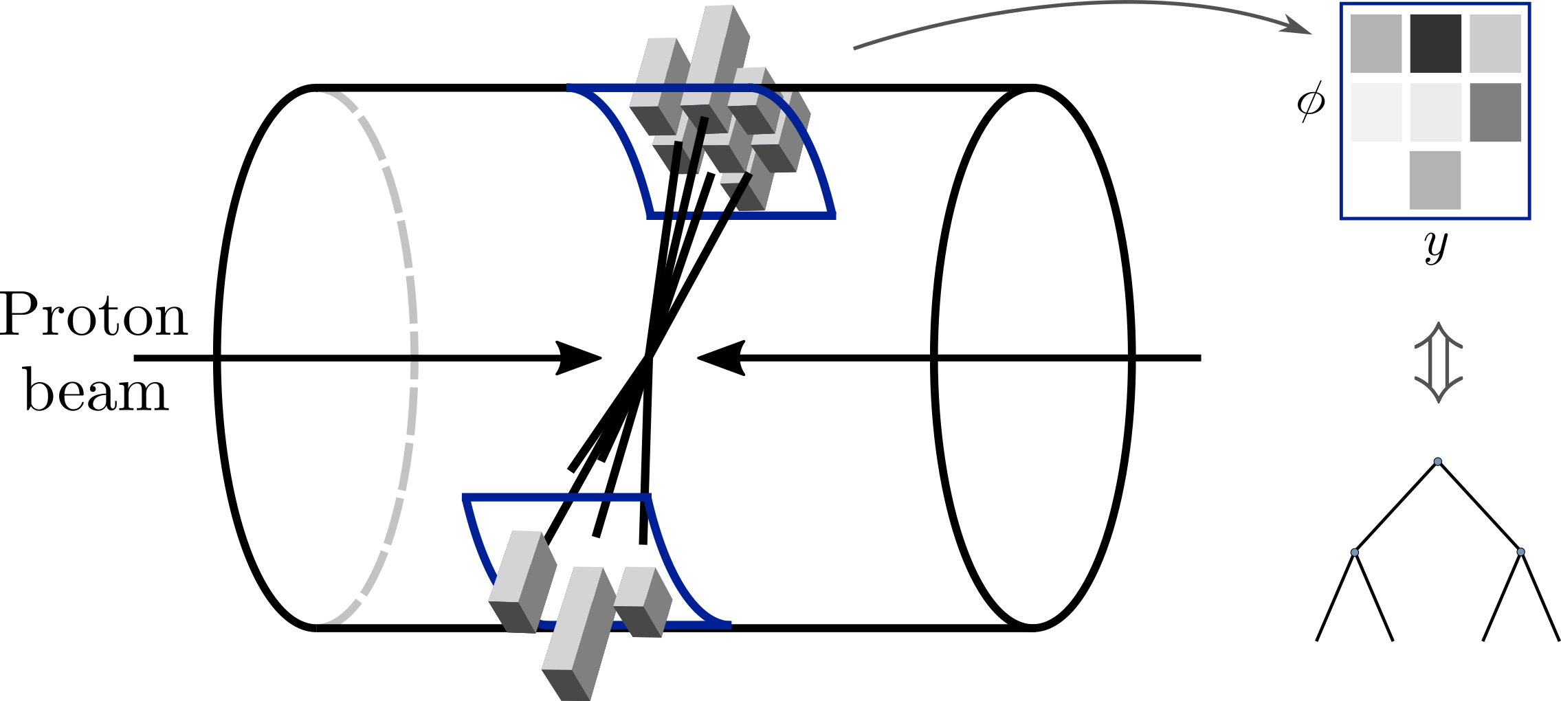
An example of an LHC collision resulting in two jets is shown in figure 1, where the towers correspond to energy deposits in the calorimeter. The right-hand side gives a schematic visualization of two different representations of jets, either as an image where the pixel intensity encodes the energy flow in that phase-space region Cogan et al. (2015), or as a tree defined by the recombination sequence of the jet algorithm.

Due to the very high energies of its collisions, the LHC is routinely producing heavy particles, such as top quarks and vector bosons, with transverse momenta far greater than their rest mass. When these objects are sufficiently energetic (or boosted), they can often generate very collimated decays, which are then reconstructed as a single fat jet. These fat jets originating from boosted objects can be distinguished from standard quark and gluon jets by studying differences in their radiation patterns. Since the advent of the LHC program, the physics of the substructure of jets has matured into a remarkably active field of research that has become notably conducive to applications of recent Machine Learning techniques Almeida et al. (2015); de Oliveira et al. (2016); Baldi et al. (2016); Guest et al. (2016); Kasieczka et al. (2017); Louppe et al. (2019); de Oliveira et al. (2017); Shimmin et al. (2017); Datta and Larkoski (2017); Larkoski et al. (2017); Pearkes et al. (2017); Butter et al. (2018); Komiske et al. (2017); Andreassen et al. (2019); Metodiev and Thaler (2018); Dreyer et al. (2018a); Komiske et al. (2019); Arjona Martínez et al. (2018); Datta et al. (2019); Butter et al. (2019); Qu and Gouskos (2019).

Figure 1: Jets emerging from a proton-proton collision at the LHC, and their representation as images in rapidity-azimuth ($y,\phi$) space or as clustering trees.

A particularly useful set of tools for experimental analyses are jet grooming algorithms Butterworth et al. (2008); Ellis et al. (2010); Krohn et al. (2010); Dasgupta et al. (2013); Larkoski et al. (2014); Dreyer et al. (2018b), defined as a post-processing treatment of jets to remove soft wide-angle radiation which is not associated with the underlying hard substructure. Grooming techniques play a crucial role in Standard Model measurements Aaboud et al. (2018); Sirunyan et al. (2018) and in improving the boson- and top-tagging efficiencies at the LHC.

In this article we introduce a novel framework, which we call GroomRL, to train a grooming algorithm using reinforcement learning (RL) Mnih et al. (2013); Silver et al. (2017). To this end, we decompose the problem of jet grooming into successive steps for which a reward function can be designed taking into account the physical features that characterize such a system. We then use a modified implementation of a Deep Q-Network (DQN) agent Mnih et al. (2013, 2015) and train a dense neural network (NN) to optimally remove radiation unassociated from the core of the jet. The trained model can then be applied on other data sets, showing improved resolution compared to state-of-the-art techniques as well as a strong resilience to non-perturbative effects. The framework and data used in this paper are available as open-source and published material in Carrazza and Dreyer (2019a, b); Carrazza and Dreyer (2019c).

Algorithm 1 Grooming

Input: policy $\pi_{g}$, binary tree node $\mathcal{T}^{(i)}$

$a_{t}=\pi_{g}(\mathcal{T}^{(i)}\rightarrow s_{t})$

if $a_{t}==1$ then

     $\mathcal{T}^{(j)}=\mathcal{T}^{(i)}$

     while $\mathcal{T}^{(j)}=(\mathcal{T}^{(j)}\rightarrow\text{parent})$ do

         $\mathcal{T}^{(j)}\rightarrow s_{t}=(\mathcal{T}^{(j)}\rightarrow s_{t})\,-\,(\mathcal{T}^{(i)}\rightarrow b\rightarrow s_{t})$

     end while

     $\mathcal{T}^{(i)}=(\mathcal{T}^{(i)}\rightarrow a)$

     Grooming($\pi_{g},\,\mathcal{T}^{(i)}$)

else

     Grooming($\pi_{g},\,\mathcal{T}^{(i)}\rightarrow a$)

     Grooming($\pi_{g},\,\mathcal{T}^{(i)}\rightarrow b$)

end if

II Jet representation

Let us start by introducing the representation we use for jets. We take the particle constituents of a jet, as defined by any modern algorithm, and recombine them using a Cambridge/Aachen (CA) sequential clustering algorithm Dokshitzer et al. (1997); Wobisch and Wengler (1998). The CA algorithm does a pairwise recombination, adding together the momenta of the two particles with the closest distance as defined by the measure

$$\Delta^{2}_{ij}=(y_{i}-y_{j})^{2}+(\phi_{i}-\phi_{j})^{2}\,,$$ (1)

where $y_{i}$ is the rapidity, a measure of relativistic velocity along the beam axis, and $\phi_{i}$ is the azimuthal angle of particle $i$ around the same axis. This clustering sequence is then used to recast the jet as a full binary tree, where each of the nodes contains information about the kinematic properties of the two parent particles. For each node $i$ of the tree we define an object $\mathcal{T}^{(i)}$ containing the current observable state $s_{t}$, as well as a pointer to the two children nodes and one to the parent node. The children nodes $a$ and $b$ are ordered in transverse momentum such that $p_{t,a}>p_{t,b}$, and we label $a$ the “harder” child and $b$ the “softer” one. The set of possible states is defined by a five-dimensional box, such that the state of the node is a tuple

$$s_{t}=\left\{z,\Delta_{ab},\psi,m,k_{t}\right\}\,,$$ (2)

where $z=p_{t,b}/(p_{t,a}+p_{t,b})$ is the momentum fraction of the softer child $b$, $\psi=\tan^{-1}\big{(}\tfrac{y_{b}-y_{a}}{\phi_{a}-\phi_{b}}\big{)}$ is the azimuthal angle around the $i$ axis, $m$ is the mass, and $k_{t}=p_{t,b}\Delta_{ab}$ is the transverse momentum of $b$ relative to $a$.

II.1 Grooming algorithm

A grooming algorithm acting on a jet tree can be defined by a simple recursive procedure which follows each of the branches and uses a policy $\pi_{g}(s_{t})$ to decide based on the values of the current tuple $s_{t}$ whether to remove the softer of the two branches. This is shown in Algorithm 1, where the minus sign is understood to mean the update of the kinematics of a node after removal of a soft branch. The grooming policy $\pi_{g}(s_{t})$ returns an action $a_{t}\in\{0,1\}$, with $a_{t}=1$ corresponding to the removal of a branch, and $a_{t}=0$ leaving the node unchanged. The state $s_{t}$ is used to evaluate the current action-values $Q^{*}(s,a)$ for each possible action, which in turn are used to determine the best action at this step through a greedy policy.

Figure 2: Example of grooming on the binary tree representation of a jet with the resulting tree after applying Algorithm 1 shown on the right. Groomed branches are indicated in red, and the corresponding nodes have been removed on the right-hand side.

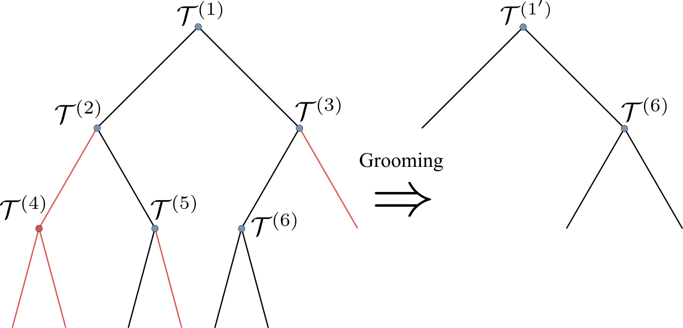
An example of the action of a grooming algorithm on a tree is shown in figure 2, where the groomed branches are indicated in red. The tree nodes whose kinematics have been modified by the removal of a branch are indicated with a prime.

It is easy to translate modern grooming algorithms in this language. For example, Recursive Soft Drop (RSD) Dreyer et al. (2018b) corresponds to a policy

$$\pi_{\text{RSD}}(s_{t})=\begin{cases}0\quad\text{if}\quad z>z_{\text{cut}}\big{(}\frac{\Delta_{ab}}{R_{0}}\big{)}^{\beta}\,,\\ 1\quad\text{else}\,,\end{cases}$$ (3)

where $z_{\text{cut}}$, $\beta$ and $R_{0}$ are the parameters of the algorithm, and $1$ corresponds as before to the action of removing the tree branch with smaller transverse momentum.

III Setting up a grooming environment

In order to find an optimal grooming policy $\pi_{g}$, we introduce an environment and a reward function, formulating the problem in a way that can be solved using a RL algorithm.

We initialize a list of all trees used for the training, from which a tree is randomly selected at the beginning of each episode. We then start by adding the root of the current tree to an empty priority queue, which orders the nodes it contains according to their $\Delta_{ab}$ value.

Each step consists in removing the first node from the priority queue, and taking an action on which of its branches to keep based on the state $s_{t}$ of that node. Once a decision has been taken on the removal of the softer branch, and the parent nodes have been updated accordingly, the remaining children of the node are added to the priority queue. The reward function is then evaluated using the current state of the tree. The episode terminates once the priority queue is empty.

The framework described here deviates from usual RL implementations in that the range of possible states for any episode are fixed at the start. The transition probability between states $\mathcal{P}(s_{t+1}|s_{t},a_{t})$ therefore does not necessarily depend very strongly on the action, although a grooming action can result in the removal of some of the future states and will therefore still have an effect on the distribution.

For our implementation, we have relied on the gym v0.12.1 Brockman et al. (2016) and keras-rl v0.4.2 Plappert (2016) libraries for the reinforcement learning component, while the neural network is set up using keras v2.2.4 Chollet et al. (2015) with TensorFlow v1.13.1 Abadi et al. (2015) as the backend.

Figure 3: Top: Loss as a function of the reward parameters, with the optimal parameters shown in red. Bottom: Value of the two terms in the Soft-Drop reward function given in equation (6) as a function of $\Delta$ and $z$.

III.1 Finding optimal hyper-parameters

The optimal choice of hyper-parameters, both for the model architecture and for the grooming parameters, is determined using the distributed asynchronous hyper-parameter optimization library hyperopt Bergstra et al. (2013).

The performance of an agent is evaluated by defining a loss function, which is evaluated on a distinct validation set consisting of 50 000 signal and background jets. For each sample, we evaluate the jet mass after grooming of each jet and derive the corresponding distribution. To calculate the loss function $\mathcal{L}$, we start by determining a window $(w_{\text{min}},w_{\text{max}})$ containing a fraction $f=0.6$ of the final jet masses of the groomed signal distribution, defining $w_{\text{med}}$ as the median value on that interval. The loss function is then defined as

$$\mathcal{L}=\frac{1}{5}|w_{\text{max}}-w_{\text{min}}|+|m_{\text{target}}-w_{\text{med}}|+20f_{\text{bkg}}\,,$$ (4)

where $f_{\text{bkg}}$ is the fraction of the groomed background sample contained in the same interval, and $m_{\text{target}}$ is a reference value for the signal.

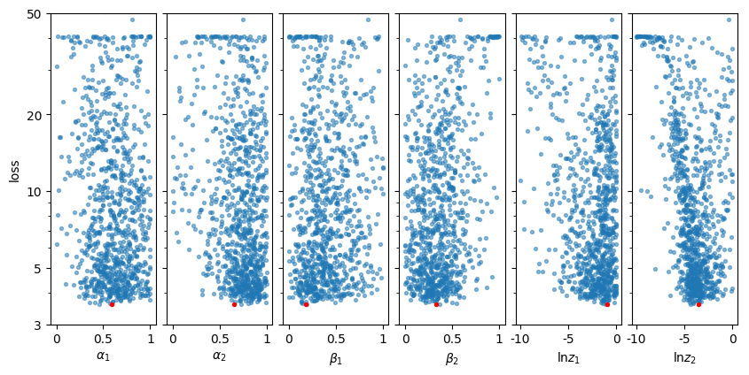
We scan hyper-parameters using 1000 iterations and select the ones for which the loss $\mathcal{L}$ evaluated on the validation set is minimal. In practice we will do three different scans: to determine the best parameters of the reward function, to find an optimal grooming environment, and to determine the architecture of the DQN agent. The scan is performed by requiring hyperopt to use a uniform search space for continuous parameters, a log-uniform search space for the learning rate and a binary choice for all integer or boolean parameters. The optimization used in all the results presented in this work rely on the Tree-structured Parzen Estimator (TPE) algorithm.

Figure 4: Distribution of the loss value for different grooming parameters. The best performing model is indicated in red.

III.2 Defining a reward function

One of the key ingredients for the optimization of the grooming policy is the reward function used at each step during the training. We consider a reward with two components: a first piece evaluated on the full tree, and another that considers only the kinematics of the current node.

The first component of the reward compares the mass of the current jet to a set target mass, typically the mass of the underlying boosted object. We implement this mass reward using a Cauchy distribution, which has two free parameters, the target mass $m_{\text{target}}$ and a width $\Gamma$, so that

$$R_{M}(m)=\frac{\Gamma^{2}}{\pi(|m-m_{\text{target}}|^{2}+\Gamma^{2})}\,.$$ (5)

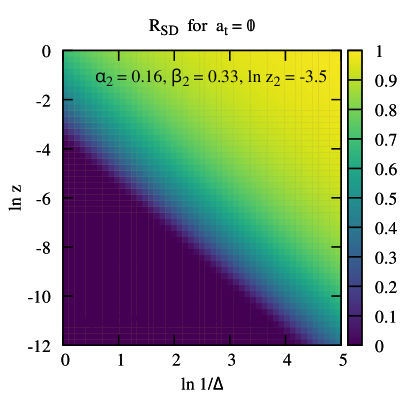
Separately, we calculate a reward on the current node which gives a positive reward for the removal of wide-angle soft radiation, as well as for leaving intact hard-collinear emissions. This provides a baseline behavior for the groomer. We label this reward component “Soft-Drop” due to its similarity with the Soft Drop condition Larkoski et al. (2014), and implement it through exponential distributions

$$R_{\text{SD}}(a_{t},\Delta,z)=a_{t}\min\big{(}1,e^{-\alpha_{1}\ln(1/\Delta)+\beta_{1}\ln(z_{1}/z)}\big{)}\\ +(1-a_{t})\max\big{(}0,1-e^{-\alpha_{2}\ln(1/\Delta)+\beta_{2}\ln(z_{2}/z)}\big{)}\,,$$ (6)

where $a_{t}=0,1$ is the action taken by the policy, and $\alpha_{i},\beta_{i},z_{i}$ are free parameters. The two terms determining $R_{\text{SD}}$ are shown in the lower panel of figure 3, using parameter values determined through asynchronous hyper-parameter optimization, shown in the upper row of the figure.

The total reward function is then given by

$$R(m,a_{t},\Delta,z)=R_{M}(m)+\frac{1}{N_{\text{SD}}}R_{\text{SD}}(a_{t},\Delta,z)\,.$$ (7)

Here $N_{\text{SD}}$ is a normalization factor determining the weight given to the second component of the reward.

III.3 RL implementation and multi-level training

For the applications in this article, we have implemented a DQN agent that contains a groomer module, which is defined by the underlying NN model and the test policy used by the agent. The groomer can be extracted after the model has been trained, using a greedy policy to select the best action based on the $Q$-values predicted by the NN. This allows for straightforward application of the resulting grooming strategy on new samples.

The training sample consists of 500 000 signal and background jets simulated using Pythia 8.223 Sjöstrand et al. (2015). We will construct two separate models by considering two signal samples, one with boosted $W$ jets and one with boosted top jets, while the background always consists of QCD jets. We use the $WW$ and $t\bar{t}$ processes, with hadronically decaying $W$ and top, to create the signal samples, and the dijet process for the background. Jets are clustered using the anti-$k_{t}$ algorithm Cacciari et al. (2008, 2012) with radius $R=1.0$, and are required to pass a selection cut, with transverse momentum $p_{t}>500$ GeV and rapidity $|y|<2.5$. All samples used in this article are available online Carrazza and Dreyer (2019c). The grooming environment is initialized by reading in the training data and creating an event array containing the corresponding jet trees.

To train the RL agent, we use a multi-level approach taking into account both signal and background samples. At the beginning of each episode, we select either a signal jet or a background jet, with probability $1-p_{\text{bkg}}$. For signal jets, the reward function uses a reference mass set to the $W$-boson mass, $m_{\text{target}}=m_{W}$, or to the top mass, $m_{\text{target}}=m_{t}$, depending on the choice of sample. In the case of the background the mass reward function in equation (7) is changed to

$$R^{\rm bkg}_{M}(m)=\frac{m}{\Gamma_{\rm bkg}}\exp\Big{(}-\frac{m}{\Gamma_{\rm bkg}}\,\Big{)}\,.$$ (8)

The width parameters $\Gamma$, $\Gamma_{\rm bkg}$ are also set to different values for signal and background reward functions, and are determined through a hyper-parameter scan.

We found that while this multi-level training only marginally improves the performance, it noticeably reduces the variability of the model.

III.4 Determining the RL agent

The DQN agent uses an Adam optimizer Kingma and Ba (2014), and the training is performed with a Boltzmann policy, which chooses an action according to weighted probabilities, with the current best action being the likeliest.

Let us now determine the remaining parameters of the DQN agent. To this end, we perform two independent scans, for the grooming environment and for the network architecture.

Figure 5: Distribution of the loss value for different architecture configurations. The best performing model is indicated in red.

The grooming environment has several options, which are shown in figure 4. Here the distribution of loss values for discrete options are displayed using violin plots, showing both the probability density of the loss values as well as its quartiles. The first plot is the dimensionality of the state observed at each step, which can be a subset of the tuple given in equation (2). We can observe that as the dimension of the input state is increased, the NN is able to leverage this additional information, leading to a decrease of the loss function. The scan over the normalization parameters of the reward functions shows that it is preferable to use a small width $\Gamma$ for the signal, with a large value $\Gamma_{\rm bkg}$ for the background, as well as a small value for the $1/N_{\rm SD}$ factor. One can also see that the multi-level training described in section III.3 leads to a distribution of loss values concentrated at smaller values. We have also allowed for several functional forms of the signal mass reward function, although for our final model we will use a Cauchy distribution.

The parameters of the network architecture are shown in figure 5, with the first plot showing the mass window containing $60\%$ of the signal distribution, with the median of that interval shown in blue. The scatter plot of the learning rate used for the Adam optimizer shows that a value slightly above $10^{-4}$ yields the best result. The scan shows a preference for a dense network with a large number of units and layers as well as a dropout layer as the architecture of the NN. Finally, we see that using duelling networks Wang et al. (2015) leads to a small improvement of the model, while double Q-learning van Hasselt et al. (2015) does not.

III.5 Optimal GroomRL model

The final GroomRL model is trained using the full training sample with 500 000 signal/background jets for 1 000 000 epochs. The overall training time requires four hours of training using a single NVIDIA GTX 1080 Ti GPU with 12 GB of memory which includes all the training jet trees and the DQN parameters.

The parameters of the best GroomRL model obtained following the strategy presented in the previous sections is listed in table 1. Here two values are given for the $m_{\rm target}$ parameter, which are used to train on either a sample consisting of $W$ bosons or of top quarks. The resulting models are labeled GroomRL-W and GroomRL-Top respectively.

x Parameters Value $m_{\rm target}$ 80.385 GeV or 173.2 GeV $s_{t}$ dimension 5 reward Cauchy $\Gamma$ 2 GeV $(\alpha_{1},\beta_{1},\ln z_{1})$ $(0.59,0.18,-0.92)$ $(\alpha_{2},\beta_{2},\ln z_{2})$ $(0.65,0.33,-3.53)$ $1/N_{\rm SD}$ 0.15 multi-level training Yes $\Gamma_{\rm bkg}$ 8 GeV $1/N_{\rm bkg}$ 1.8 or 1.0 $p_{\rm bkg}$ 0.48 or 0.2 learning rate $10^{-4}$ Dueling NN Yes Double DQN No Policy Boltzmann $N_{\rm epochs}^{\rm max}$ 500 000 Architecture Dense Dropout 0.05 Layers 10 Nodes 100 Optimizer Adam

Table 1: Final parameters for GroomRL, with the two values of $m_{\rm target}$ corresponding to the $W$ and top mass.

Figure 6: Reward evolution during training of the GroomRL on $W$ and top data. A LOESS smoothing is applied to the original curves.

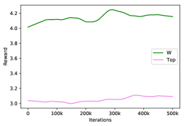
In figure 6 we show the reward value during the training of the GroomRL for $W$ bosons and top quarks, after applying the LOESS smoothing algorithm on the original curve. We observe an improvement of the reward function during the first 300 000 training epochs, with the reward becoming relatively stable after that point.

III.6 Alternative approaches

In this section, we have introduced a novel implementation of RL to tackle the problem of tree pruning. A number of alternative methods could be studied to approach this problem, most notably Monte-Carlo Tree Search (MCTS) algorithms Coulom (2007); Kocsis and Szepesvári (2006) and binary classifiers. The heuristic search methods from MCTS explore the tree through random sampling, taking random actions to progress through the tree. Once an endpoint is reached, the result is used to weight the nodes and improve future decisions.

More recently, a NN based MCTSnet implementation was proposed Guez et al. (2018), which introduces a framework to learn how to search the tree, integrating simulation-based planning into a NN.

These techniques might provide an interesting basis to construct an efficient groomer. However due to the wide variability of the trees considered in our case study, where each new episode starts from a unique tree, this would require a substantial modification of the algorithm.

Alternatively, one could use a contextual bandit solver Auer et al. (2003); Agarwal et al. (2014) to train a jet grooming policy. We would expect this method to yield similar results, however, this method does not allow for the modification of the future nodes by the current grooming decision, and is not as easily extendable as our current framework.

Finally, one could attempt to build a jet grooming algorithm from a binary classifier, which uses an input state to determine which action to take next. The main drawback of this method is that one can not straightforwardly impose as loss function the mass resolution of the tree, as this depends on previous states of the current episode. As such, the problem we consider is particularly well adapted to a RL approach.

We leave a more thorough study of the application of these alternative tools to jet grooming for future work.

IV Jet mass spectrum

Let us now apply the GroomRL models defined in section III.5 to new data samples. We consider three test sets of 50 000 elements each: one with QCD jets, one with $W$ initiated jets and one with top jets. The size of the window containing $60\%$ of the mass spectrum of the $W$ sample, as well as the corresponding median value, are given in table 2 for each different grooming strategy. As a benchmark, we compare to the RSD algorithm, using parameters $z_{\text{cut}}=0.05$, $\beta=1$ and $R_{0}=1$. One can notice a sizeable reduction of the window size after grooming with the machine learning based algorithms, while all groomers are able to reconstruct the peak location to a value very close to the $W$ mass.

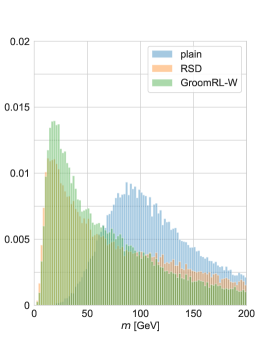
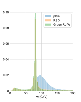
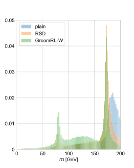
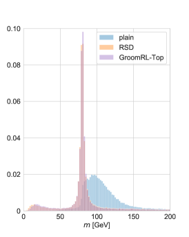
The distribution of the jet mass after grooming for each of these samples is shown in figures 7 and 8. Each curve gives the differential cross section $d\sigma/dm_{j}$ normalized by the total cross section. Figure 7 shows results for the grooming algorithm trained on a $W$ sample, while the results of the algorithm trained on top data are given in figure 8. As references, the ungroomed (or plain) jet mass and the jet mass after RSD grooming are also given, in blue and orange respectively. As expected, one can observe that for the ungroomed case the resolution is very poor, with the QCD jets having large masses due to wide-angle radiation, while the $W$ and top mass peaks are heavily distorted. In contrast, after applying RSD or GroomRL, the jet mass is reconstructed much more accurately. One interesting feature of GroomRL is that it is able to lower the jet mass for quark and gluon jets, further reducing the background contamination in windows close to a heavy particle mass.

For the $W$ case, shown in figures 7b and 8b, there is a sharp peak around the $W$ mass $m_{W}$, with the GroomRL method providing slightly better resolution. It is also particularly noteworthy that both the GroomRL-W and the GroomRL-Top algorithms have similar performance, despite the latter one having been trained on a completely different data set. This demonstrates that the tools derived from our framework are robust and can be applied to data sets beyond their training range with good results.

(a) QCD

(b) W

(c) top

Figure 7: Groomed jet mass spectrum for (a) QCD jets, (b) $W$ jets, (c) top jets. The GroomRL-W curve is obtained from training on $W$ data.

x $w_{\text{max}}-w_{\text{min}}$ [GeV] $w_{\text{med}}$ [GeV] plain $44.65$ $104.64$ GroomRL-W $10.70$ $80.09$ GroomRL-Top $13.88$ $80.46$ RSD $16.96$ $80.46$

Table 2: Size of the window containing $60\%$ of the $W$ mass spectrum, and median value on that interval.

(a) QCD

(b) W

(c) top

Figure 8: Groomed jet mass spectrum for (a) QCD jets, (b) $W$ jets, (c) top jets. The GroomRL-Top curve is obtained from training on top data.

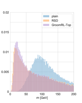
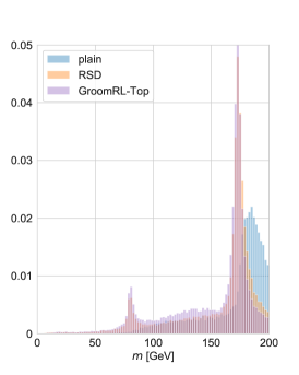
In top jets, displayed in figures 7c and 8c, the enhancements are even more noticeable. Here again, the performance of both algorithms is similar, despite the fact that the training of GroomRL-W did not involve any top-related data.

(a) Plain

(b) GroomRL-W

(c) GroomRL-Top

Figure 9: Primary Lund jet plane density for QCD jets before (a) and after grooming with GroomRL trained on $W$ (b) or top (c) samples.

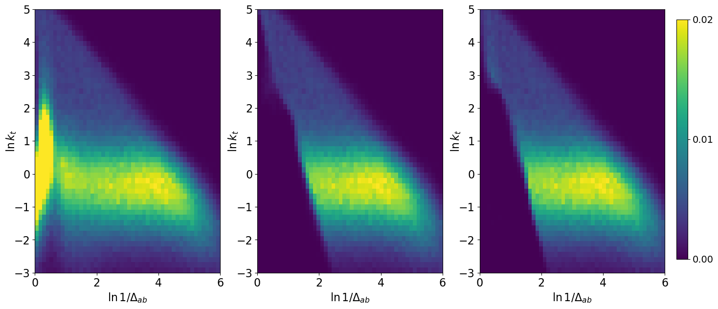
Finally, in figure 9, we show the primary Lund jet plane density as defined in Dreyer et al. (2018a) after grooming with GroomRL-W and GroomRL-Top, averaged over 50 000 jets. This gives a useful visualization of radiation patterns within a jet, providing a physical interpretation of the grooming behavior. The primary Lund jet plane is defined through the $(\ln 1/\Delta_{ab},\ln k_{t})$ coordinates of each of the states of the “primary” declustering sequence, i.e. traversing the jet tree by successively following the hardest branch $\mathcal{T}^{(i)}\rightarrow a$. The upper boundary of the triangle is due to the kinematic limit of emissions. In contrast, the lower edge corresponds to radiation that gets removed by the grooming algorithm, so that only sufficiently energetic or collinear partons remain in the groomed jet.

An interesting feature of figure 9 is that can one observe that despite producing similar jet mass spectra, the GroomRL-W and GroomRL-Top algorithms differ somewhat, with the former retaining more radiation at wide angles than the latter.

IV.1 Robustness to non-perturbative effects

Let us now consider the impact of non-perturbative effects such as hadronization and underlying event on groomed jets. A key feature of grooming algorithms such as mMDT and Soft Drop is that they reduce the sensitivity of observables to non-perturbative effects, allowing for precise comparisons between theoretical predictions and experimental measurements.

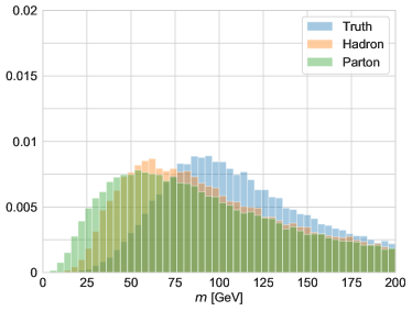
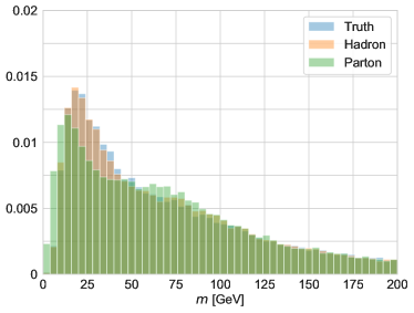
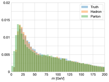
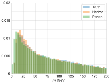
To study the robustness of GroomRL to these contributions, we consider three different QCD jet samples generated through Pythia’s dijet process. The first one, which we denote as “truth-level” and used already in the previous sections, includes all non-perturbative effects. A “hadron-level” sample is obtained by removing multiple parton interactions from the simulation, and finally a “parton-level” sample is generated by further turning off the hadronization step in Pythia.

The jet mass spectrum for each sample is shown in figure 10, with results for ungroomed jets as well as after grooming with GroomRL-W, GroomRL-Top and RSD. One can see immediately that the ungroomed jet mass spectrum is strongly affected by non-perturbative effects, while groomed jets become much more robust to these contributions. For masses $m>50$ GeV, both GroomRL models become very robust, showing a resilience to hadronization and underlying event similar to that of RSD. In the low mass range, GroomRL remains robust to multiple parton interactions, but starts to show some dependence on hadronization effects.

We note that no parton-level or hadron-level data was used in the training, such that one would not a priori expect the derived algorithm to be particularly resilient to these effects. Although GroomRL already performs surprisingly well, one could easily further improve the robustness of the model by including some of this data with a suitable modification of the reward function in the training of the DQN agent.

(a) Plain

(b) GroomRL-W

(c) GroomRL-Top

(d) RSD

Figure 10: Jet mass spectrum for QCD jets at parton-level (green), hadron-level (orange) and including underlying event (blue). Distributions are shown for ungroomed jets (a), as well as after grooming with GroomRL trained on $W$ data (b), on top data (c) or with RSD (d).

V Conclusions

We have shown a promising application of RL to the issue of jet grooming. Using a carefully designed reward function, we have constructed a groomer from a dense NN trained with a DQN agent.

This grooming algorithm was then applied to a range of data samples, showing excellent results for the mass resolution of boosted heavy particles. In particular, while the training of the NN is performed on samples consisting of $W$ (or top) jets, the groomer yields noticeable gains in the top (or $W$) case as well, on data outside of the training range.

The improvements in resolution and background reduction compared to alternative state-of-the-art methods provide an encouraging demonstration of the relevance of machine learning for jet grooming. In particular, we showed that it is possible for a RL agent to extract the underlying physics of jet grooming and distill this knowledge into an efficient algorithm.

Due to its simplicity, the model we developed also retains most of the calculability of other existing methods such as Soft Drop. Accurate numerical computations of groomed jet observables are therefore achievable, allowing for the possibility of direct comparisons with data. Furthermore, given an appropriate sample, one could also attempt to train the grooming strategy on real data, bypassing some of the limitations due to the use of parton shower programs.

The GroomRL framework, available online Carrazza and Dreyer (2019a, b), is generic and can easily be extended to higher-dimensional inputs, for example to consider multiple emissions per step or additional kinematic information. While the method presented in this article was applied to a specific problem in particle physics, we expect that with a suitable choice of reward function, this framework is in principle also applicable to a range of problems where a tree requires pruning.

Acknowledgments: We are grateful to Jia-Jie Zhu and Gavin Salam for comments on the manuscript and to Jesse Thaler for useful discussions. We also acknowledge the NVIDIA Corporation for the donation of a Titan Xp GPU used for this research. F.D. is supported by the Science and Technology Facilities Council (STFC) under grant ST/P000770/1. S.C. is supported by the European Research Council under the European Union’s Horizon 2020 research and innovation Programme (grant agreement number 740006).

References

- Sterman and Weinberg (1977) G. F. Sterman and S. Weinberg, Phys. Rev. Lett. 39, 1436 (1977).
- Salam (2010) G. P. Salam, Eur. Phys. J. C67, 637 (2010), eprint 0906.1833.
- Ellis and Soper (1993) S. D. Ellis and D. E. Soper, Phys. Rev. D48, 3160 (1993), eprint hep-ph/9305266.
- Dokshitzer et al. (1997) Y. L. Dokshitzer, G. D. Leder, S. Moretti, and B. R. Webber, JHEP 08, 001 (1997), eprint hep-ph/9707323.
- Cacciari et al. (2008) M. Cacciari, G. P. Salam, and G. Soyez, JHEP 04, 063 (2008), eprint 0802.1189.
- Cogan et al. (2015) J. Cogan, M. Kagan, E. Strauss, and A. Schwarztman, JHEP 02, 118 (2015), eprint 1407.5675.
- Almeida et al. (2015) L. G. Almeida, M. Backović, M. Cliche, S. J. Lee, and M. Perelstein, JHEP 07, 086 (2015), eprint 1501.05968.
- de Oliveira et al. (2016) L. de Oliveira, M. Kagan, L. Mackey, B. Nachman, and A. Schwartzman, JHEP 07, 069 (2016), eprint 1511.05190.
- Baldi et al. (2016) P. Baldi, K. Bauer, C. Eng, P. Sadowski, and D. Whiteson, Phys. Rev. D93, 094034 (2016), eprint 1603.09349.
- Guest et al. (2016) D. Guest, J. Collado, P. Baldi, S.-C. Hsu, G. Urban, and D. Whiteson, Phys. Rev. D94, 112002 (2016), eprint 1607.08633.
- Kasieczka et al. (2017) G. Kasieczka, T. Plehn, M. Russell, and T. Schell, JHEP 05, 006 (2017), eprint 1701.08784.
- Louppe et al. (2019) G. Louppe, K. Cho, C. Becot, and K. Cranmer, JHEP 01, 057 (2019), eprint 1702.00748.
- de Oliveira et al. (2017) L. de Oliveira, M. Paganini, and B. Nachman, Comput. Softw. Big Sci. 1, 4 (2017), eprint 1701.05927.
- Shimmin et al. (2017) C. Shimmin, P. Sadowski, P. Baldi, E. Weik, D. Whiteson, E. Goul, and A. Søgaard, Phys. Rev. D96, 074034 (2017), eprint 1703.03507.
- Datta and Larkoski (2017) K. Datta and A. Larkoski, JHEP 06, 073 (2017), eprint 1704.08249.
- Larkoski et al. (2017) A. J. Larkoski, I. Moult, and B. Nachman (2017), eprint 1709.04464.
- Pearkes et al. (2017) J. Pearkes, W. Fedorko, A. Lister, and C. Gay (2017), eprint 1704.02124.
- Butter et al. (2018) A. Butter, G. Kasieczka, T. Plehn, and M. Russell, SciPost Phys. 5, 028 (2018), eprint 1707.08966.
- Komiske et al. (2017) P. T. Komiske, E. M. Metodiev, B. Nachman, and M. D. Schwartz, JHEP 12, 051 (2017), eprint 1707.08600.
- Andreassen et al. (2019) A. Andreassen, I. Feige, C. Frye, and M. D. Schwartz, Eur. Phys. J. C79, 102 (2019), eprint 1804.09720.
- Metodiev and Thaler (2018) E. M. Metodiev and J. Thaler, Phys. Rev. Lett. 120, 241602 (2018), eprint 1802.00008.
- Dreyer et al. (2018a) F. A. Dreyer, G. P. Salam, and G. Soyez, JHEP 12, 064 (2018a), eprint 1807.04758.
- Komiske et al. (2019) P. T. Komiske, E. M. Metodiev, and J. Thaler, JHEP 01, 121 (2019), eprint 1810.05165.
- Arjona Martínez et al. (2018) J. Arjona Martínez, O. Cerri, M. Pierini, M. Spiropulu, and J.-R. Vlimant (2018), eprint 1810.07988.
- Datta et al. (2019) K. Datta, A. Larkoski, and B. Nachman (2019), eprint 1902.07180.
- Butter et al. (2019) A. Butter et al. (2019), eprint 1902.09914.
- Qu and Gouskos (2019) H. Qu and L. Gouskos (2019), eprint 1902.08570.
- Butterworth et al. (2008) J. M. Butterworth, A. R. Davison, M. Rubin, and G. P. Salam, Phys. Rev. Lett. 100, 242001 (2008), eprint 0802.2470.
- Ellis et al. (2010) S. D. Ellis, C. K. Vermilion, and J. R. Walsh, Phys. Rev. D81, 094023 (2010), eprint 0912.0033.
- Krohn et al. (2010) D. Krohn, J. Thaler, and L.-T. Wang, JHEP 02, 084 (2010), eprint 0912.1342.
- Dasgupta et al. (2013) M. Dasgupta, A. Fregoso, S. Marzani, and G. P. Salam, JHEP 09, 029 (2013), eprint 1307.0007.
- Larkoski et al. (2014) A. J. Larkoski, S. Marzani, G. Soyez, and J. Thaler, JHEP 05, 146 (2014), eprint 1402.2657.
- Dreyer et al. (2018b) F. A. Dreyer, L. Necib, G. Soyez, and J. Thaler, JHEP 06, 093 (2018b), eprint 1804.03657.
- Aaboud et al. (2018) M. Aaboud et al. (ATLAS), Phys. Rev. Lett. 121, 092001 (2018), eprint 1711.08341.
- Sirunyan et al. (2018) A. M. Sirunyan et al. (CMS), JHEP 11, 113 (2018), eprint 1807.05974.
- Mnih et al. (2013) V. Mnih, K. Kavukcuoglu, D. Silver, A. Graves, I. Antonoglou, D. Wierstra, and M. A. Riedmiller, CoRR abs/1312.5602 (2013), eprint 1312.5602, URL http://arxiv.org/abs/1312.5602.
- Silver et al. (2017) D. Silver, J. Schrittwieser, K. Simonyan, I. Antonoglou, A. Huang, A. Guez, T. Hubert, L. Baker, M. Lai, A. Bolton, et al., Nature 550, 354 (2017), URL http://dx.doi.org/10.1038/nature24270.
- Mnih et al. (2015) V. Mnih, K. Kavukcuoglu, D. Silver, A. A. Rusu, J. Veness, M. G. Bellemare, A. Graves, M. Riedmiller, A. K. Fidjeland, G. Ostrovski, et al., Nature 518, 529 (2015), ISSN 00280836, URL http://dx.doi.org/10.1038/nature14236.
- Carrazza and Dreyer (2019a) S. Carrazza and F. A. Dreyer, JetsGame/GroomRL v1.0.0 (2019a), URL https://doi.org/10.5281/zenodo.2602529.
- Carrazza and Dreyer (2019b) S. Carrazza and F. A. Dreyer, JetsGame/libGroomRL v1.0.0 (2019b), URL https://doi.org/10.5281/zenodo.3265835.
- Carrazza and Dreyer (2019c) S. Carrazza and F. A. Dreyer, JetsGame/data v1.0.0 (2019c), this repository is git-lfs., URL https://doi.org/10.5281/zenodo.2602514.
- Wobisch and Wengler (1998) M. Wobisch and T. Wengler, in Monte Carlo generators for HERA physics. Proceedings, Workshop, Hamburg, Germany, 1998-1999 (1998), pp. 270–279, eprint hep-ph/9907280.
- Brockman et al. (2016) G. Brockman, V. Cheung, L. Pettersson, J. Schneider, J. Schulman, J. Tang, and W. Zaremba, Openai gym (2016), eprint arXiv:1606.01540.
- Plappert (2016) M. Plappert, keras-rl, https://github.com/keras-rl/keras-rl (2016).
- Chollet et al. (2015) F. Chollet et al., Keras, https://keras.io (2015).
- Abadi et al. (2015) M. Abadi et al., TensorFlow: Large-scale machine learning on heterogeneous systems (2015), software available from tensorflow.org, URL https://www.tensorflow.org/.
- Bergstra et al. (2013) J. Bergstra, D. Yamins, and D. D. Cox, in Proceedings of the 30th International Conference on International Conference on Machine Learning - Volume 28 (JMLR.org, 2013), ICML’13, pp. I–115–I–123.
- Sjöstrand et al. (2015) T. Sjöstrand, S. Ask, J. R. Christiansen, R. Corke, N. Desai, P. Ilten, S. Mrenna, S. Prestel, C. O. Rasmussen, and P. Z. Skands, Comput. Phys. Commun. 191, 159 (2015), eprint 1410.3012.
- Cacciari et al. (2012) M. Cacciari, G. P. Salam, and G. Soyez, Eur. Phys. J. C72, 1896 (2012), eprint 1111.6097.
- Kingma and Ba (2014) D. P. Kingma and J. Ba, CoRR abs/1412.6980 (2014), eprint 1412.6980, URL http://arxiv.org/abs/1412.6980.
- Wang et al. (2015) Z. Wang, N. de Freitas, and M. Lanctot, CoRR abs/1511.06581 (2015), eprint 1511.06581, URL http://arxiv.org/abs/1511.06581.
- van Hasselt et al. (2015) H. van Hasselt, A. Guez, and D. Silver, CoRR abs/1509.06461 (2015), eprint 1509.06461, URL http://arxiv.org/abs/1509.06461.
- Coulom (2007) R. Coulom, in Proceedings of the 5th International Conference on Computers and Games (Springer-Verlag, Berlin, Heidelberg, 2007), CG’06, pp. 72–83.
- Kocsis and Szepesvári (2006) L. Kocsis and C. Szepesvári, in Machine Learning: ECML 2006 (Springer, 2006), pp. 282–293.
- Guez et al. (2018) A. Guez, T. Weber, I. Antonoglou, K. Simonyan, O. Vinyals, D. Wierstra, R. Munos, and D. Silver, in ICML (2018).
- Auer et al. (2003) P. Auer, N. Cesa-Bianchi, Y. Freund, and R. E. Schapire, SIAM J. Comput. 32, 48 (2003), ISSN 0097-5397, URL https://doi.org/10.1137/S0097539701398375.
- Agarwal et al. (2014) A. Agarwal, D. J. Hsu, S. Kale, J. Langford, L. Li, and R. E. Schapire, CoRR abs/1402.0555 (2014), eprint 1402.0555, URL http://arxiv.org/abs/1402.0555.