Principal components in linear mixed models with general bulk

Abstract.

We study the principal components of covariance estimators in multivariate mixed-effects linear models. We show that, in high dimensions, the principal eigenvalues and eigenvectors may exhibit bias and aliasing effects that are not present in low-dimensional settings. We derive the first-order limits of the principal eigenvalue locations and eigenvector projections in a high-dimensional asymptotic framework, allowing for general population spectral distributions for the random effects and extending previous results from a more restrictive spiked model. Our analysis uses free probability techniques, and we develop two general tools of independent interest—strong asymptotic freeness of GOE and deterministic matrices and a free deterministic equivalent approximation for bilinear forms of resolvents.

1. Introduction

Principal components analysis (PCA) is a commonly used technique for identifying linear low-rank structure in high-dimensional data [Jol11]. For $n$ independent samples in a comparably large dimension $p$, it is now well-established that the principal components of the sample covariance matrix may be inaccurate for their population counterparts [JL09]. A body of work has quantified the behavior of PCA in this setting [Joh01, BBP05, BS06, Pau07, BGN12, BY12], connecting to the Marcenko-Pastur and Tracy-Widom laws of asymptotic random matrix theory [MP67, TW96]. We refer readers to the review articles [PA14, JP18] for more discussion and references to this and related lines of work.

Similar phenomena occur in statistical models where samples are not independent, but instead exhibit complex dependence structure [BJW05, Zha06, LAP15, WAP17]. However, the behavior of PCA in many such models is less well-understood. In this work, we consider the setting of mixed effects linear models [SCM09], where dependence across observed samples arises via linear combinations of independent latent variables. These models are commonly used in statistical genetics to model quantitative phenotypes in related individuals [LW98]. We study the behavior of principal eigenvalues and eigenvectors of MANOVA covariance estimates for the random effects.

Our main results quantify several spectral bias and aliasing phenomena that may occur in high-dimensional applications. In particular, we show that large principal eigenvalues in the covariance of one random effect may bias the principal eigenvectors and also yield spurious eigenvalues in the estimated covariances of the other effects. These phenomena are unique to mixed-effects models, and they do not arise in similar spiked models of sample covariance matrices for independent samples [BBP05, BS06, Pau07]. In [FJS18], such phenomena for mixed models were first described under an “isotropic noise” assumption, where the population covariance of each random effect is a low-rank perturbation of the identity. Our work extends these results to the setting of general population spectral distributions for the random effects. We derive generalizations of the first-order limits for eigenvalues and eigenvector projections in [FJS18] involving quantities appearing in the fixed-point equations for the empirical spectral law in [FJ19]. We describe these results in Section 2.

Our proofs are very different from the analytic approach of [FJS18]. Instead, they are based in free probability theory and its connection to random matrices [Voi91, MS17]. Our work also establishes two general results in this area—strong asymptotic freeness of independent GOE and deterministic matrices and a method of deriving anisotropic resolvent approximations using free deterministic equivalents [SV12]. We describe these in Section 4.

The connection between free probability and random matrices was introduced in [Voi91] for deterministic and GUE matrices and has been extended to many other matrix models [Dyk93, Voi98, HP00, Col03, CC04, CŚ06, BG09, SV12]. Strong asymptotic freeness extending the approximation from the trace to the operator norm was first proven in [HT05] for GUE matrices and extended to other models in [Sch05, CDM07, Mal12, BC17]. Free probability techniques have recently been applied to study outlier eigenvalues in other matrix models [BBCF17, BBC17] and spectral behavior in other statistical applications, including autocovariance estimates for high-dimensional time series [BB16a, BB16b, BB17, BB18, BB19] and sketching methods for linear regression [DL18]. The tools we develop may be of broader interest to the analysis of structured random matrices arising in other applications.

2. Probabilistic results in the linear mixed model

Extending the representation of [Rao72] to a multivariate setting, we consider the mixed-effects linear model

$$Y=X\beta+U_{1}\alpha_{1}+\ldots+U_{k}\alpha_{k}\in\mathbb{R}^{n\times p}$$ (1)

where $Y$ contains $n$ dependent observations in dimension $p$, each a combination of fixed effects $X\beta$ and random effects constituting the rows of $\alpha_{1},\ldots,\alpha_{k}$. Here,

• $X\in\mathbb{R}^{n\times m}$ is an observed design matrix of a small number $m$ of fixed effects, with unknown regression coefficients $\beta\in\mathbb{R}^{m\times p}$.

• For each $r=1,\ldots,k$, the matrix $\alpha_{r}\in\mathbb{R}^{n_{r}\times p}$ is unobserved, its rows constituting $n_{r}$ i.i.d. realizations of a $p$-dimensional random effect.

• Each $U_{r}\in\mathbb{R}^{n\times n_{r}}$ is a known, deterministic incidence matrix specified by the model design.

We study the behavior of PCA for estimates of the variance components, which are the covariance matrices $\Sigma_{1},\ldots,\Sigma_{k}$ for the random effects in $\alpha_{1},\ldots,\alpha_{k}$.

In quantitative genetics, $U_{1},\ldots,U_{k}$ may encode a classification design, as commonly used in twin/sibling studies and breeding experiments. Examples are discussed in [FJ19, FJS18]. In genomewide association study designs, $U_{1},\ldots,U_{k}$ may contain genotype measurements at a set of single-nucleotide polymorphisms (SNPs) [YLGV11, ZS12]. It has been recognized since [Fis18, Wri35] that variance components in these models can provide a decomposition of the total population variance of quantitative phenotypes into constituent genetic and non-genetic effects, yielding estimates of heritability. In high-dimensional applications, including the analysis of gene expression traits and other molecular phenotypes, the principal eigenvectors of the genetic components may indicate phenotypic subspaces near which responses to selection or random mutational drift are likely to be constrained [HB06, BM15, CMA⁺18]. Principal eigenvectors of the non-genetic components may correspond to hidden experimental confounders, to be removed before performing downstream analyses [LS07, SPP⁺12].

As $\alpha_{1},\ldots,\alpha_{k}$ are not individually observed, one cannot construct the usual sample covariance estimator for $\Sigma_{1},\ldots,\Sigma_{k}$. Instead, each $\Sigma_{r}$ may be classically estimated by a MANOVA estimator of the form

$$\widehat{\Sigma}_{r}=Y^{\mathsf{T}}B_{r}Y,$$

where the symmetric matrix $B_{r}$ is chosen to satisfy the properties

$$B_{r}X=0,\qquad\mathbb{E}[Y^{\mathsf{T}}B_{r}Y]=\Sigma_{r}.$$

Such an estimator $\widehat{\Sigma}_{r}$ is unbiased and equivariant to rotations of coordinates in $\mathbb{R}^{p}$—these properties are analogous to those holding for a sample covariance matrix for independent samples. For example, in a balanced one-way classification design, the within-group covariance matrix $\Sigma_{1}$ is estimated by the MANOVA estimator $\widehat{\Sigma}_{1}=Y^{\top}B_{1}Y$ where $B_{1}$ is a scaled difference of two orthogonal projections, the first onto a subspace of group means and the second onto its orthogonal complement. See Appendix A.2 for further details of this example.

Our main results, Theorems 2.5 and 2.6 below, characterize the first-order limiting behavior of the principal eigenvalues and eigenvectors of any such matrix $\widehat{\Sigma}=Y^{\top}BY$ in a high-dimensional asymptotic framework.

2.1. Model assumptions

We assume that the random effects arise in the following way.

Assumption 2.1.

The matrices $\alpha_{1},\ldots,\alpha_{k}$ are independent. The rows of each $\alpha_{r}$ are independent, with the $i^{\text{th}}$ row given by

$$\sum_{j=1}^{\ell_{r}}\gamma_{j}^{(r)}\xi_{ij}^{(r)}+\varepsilon_{i}^{(r)}.$$

Here $\gamma_{1}^{(r)},\ldots,\gamma_{\ell_{r}}^{(r)}\in\mathbb{R}^{p}$ are $\ell_{r}$ deterministic vectors, and $\xi_{ij}^{(r)}\in\mathbb{R}$ are independent random variables satisfying

$$\mathbb{E}[\xi_{ij}^{(r)}]=0,\qquad\mathbb{E}[(\xi_{ij}^{(r)})^{2}]=1,\qquad\mathbb{E}[|\xi_{ij}^{(r)}|^{k}]\leq C_{k}$$

for all $k\geq 1$ and some constants $C_{k}>0$. For a covariance $\mathring{\Sigma}_{r}\in\mathbb{R}^{p\times p}$, the noise $\varepsilon_{i}^{(r)}\in\mathbb{R}^{p}$ is Gaussian with distribution $\varepsilon_{i}^{(r)}\sim\mathcal{N}(0,\mathring{\Sigma}_{r})$.

Stacking $\gamma_{1}^{(r)},\ldots,\gamma_{\ell_{r}}^{(r)}$ as the rows of

$$\Gamma_{r}=\begin{pmatrix}-&\gamma_{1}^{(r)}&-\\ &\vdots&\\ -&\gamma_{\ell_{r}}^{(r)}&-\end{pmatrix}\in\mathbb{R}^{\ell_{r}\times p},$$ (2)

each $\alpha_{r}$ has independent rows with mean 0 and covariance of the spiked form

$$\Sigma_{r}=\Gamma_{r}^{\mathsf{T}}\Gamma_{r}+\mathring{\Sigma}_{r}.$$ (3)

The leading term $\Gamma_{r}^{\mathsf{T}}\Gamma_{r}$ induces up to $\ell_{r}$ “signal” eigenvalues that separate from the “noise” eigenvalues of $\mathring{\Sigma}_{r}$. Our results should be interpreted in the setting where the noise covariance $\mathring{\Sigma}_{r}$ does not itself have isolated eigenvalues that separate from the bulk of its eigenvalue distribution.

As a compromise between generality of the model and simplicity of the analysis, Assumption 2.1 follows the approach in [Nad08] and imposes a Gaussian assumption on $\varepsilon_{i}^{(r)}$ but not on $\xi_{ij}^{(r)}$. The signal directions $\gamma_{1}^{(r)},\ldots,\gamma_{\ell_{r}}^{(r)}$ are not required to be orthogonal for each $r$. It is likely that our theoretical results in Theorems 2.4, 2.5, and 2.6 all remain correct under a milder moment assumption for this noise $\varepsilon_{i}^{(r)}$, and it may be possible to prove such an extension using cumulant expansions of the remainder terms in the Gaussian integration-by-parts formula, as done in [BC17]. However, we will not pursue this direction in the current work.

For the linear mixed model (1), we study an asymptotic framework summarized as follows.

Assumption 2.2.

The dimensions $n,p,n_{1},\ldots,n_{k}\to\infty$, where $k$ is a fixed constant. There are universal constants $C,c>0$ such that for each $r=1,\ldots,k$,

• $c<p/n<C$ and $c<n_{r}/n<C$,

• $\|U_{r}\|<C$ and $\|B\|<C/n$

• $\|\Gamma_{r}\|<C$, $\|\mathring{\Sigma}_{r}\|<C$, and $\ell_{r}<C$.

Thus, the number of samples is proportional to the number of realizations of each random effect (and also to the dimension $p$). This and the assumption $\|U_{r}\|<C$ are discussed in greater detail in [FJ19, FJS18], and hold for many classification and experimental designs. The scaling $\|B\|<C/n$ is usual for MANOVA estimators, to yield $\widehat{\Sigma}_{r}$ on the same scale as its estimand $\Sigma_{r}$.

The last statement implies a bounded number of signal eigenvalues in each variance component, where each eigenvalue remains bounded in size. It is an important open problem to extend our results beyond this setting.

2.2. Bulk eigenvalue distribution

Under the above assumptions, a characterization of a deterministic approximation for the empirical eigenvalue distribution of

$$\widehat{\Sigma}=Y^{\top}BY$$ (4)

was derived in [FJ19]. We review this result here.

Consider the setting of no signal, meaning $\ell_{r}=0$ and $\Sigma_{r}=\mathring{\Sigma}_{r}$ for each $r=1,\ldots,k$. We introduce the notations $n_{+}=n_{1}+\cdots+n_{k}$ and

$$F_{rs}=\sqrt{n_{r}n_{s}}U_{r}^{\mathsf{T}}BU_{s}\in\mathbb{R}^{n_{r}\times n_{s}},\quad F=(F_{rs})_{r,s=1}^{k}\in\mathbb{R}^{n_{+}\times n_{+}},$$ (5)

$$\operatorname{diag}_{n}(\mathbf{a})=\operatorname{diag}(a_{1}\operatorname{Id}_{n_{1}},\ldots,a_{k}\operatorname{Id}_{n_{k}})\in\mathbb{R}^{n_{+}\times n_{+}},$$

$$\mathbf{b}\cdot\mathring{\Sigma}=b_{1}\mathring{\Sigma}_{1}+\cdots+b_{k}\mathring{\Sigma}_{k}\in\mathbb{R}^{p\times p}.$$

Let $\operatorname{Tr}_{r}$ be the trace of the $(r,r)$ block (of size $n_{r}\times n_{r}$) in the $k\times k$ matrix block decomposition corresponding to $\mathbb{C}^{n_{+}}=\mathbb{C}^{n_{1}}\oplus\cdots\oplus\mathbb{C}^{n_{k}}$. The Stieltjes transform of a measure $\mu$ is $m(z)=\int(x-z)^{-1}d\mu(x)$.

Theorem 2.3 ([FJ19]).

Suppose Assumptions 2.1 and 2.2 hold, and $\ell_{r}=0$ for each $r=1,\ldots,k$. Let $\widehat{\Sigma}$ be as in (4), and let $\widehat{\mu}=p^{-1}\sum_{i=1}^{p}\delta_{\lambda_{i}(\widehat{\Sigma})}$ be the empirical distribution of its eigenvalues.

For each $z\in\mathbb{C}^{+}$, there exist unique $z$-dependent values $a_{1},\ldots,a_{k}\in\mathbb{C}^{+}\cup\{0\}$ and $b_{1},\ldots,b_{k}\in\overline{\mathbb{C}^{+}}$ that satisfy the equations

$$a_{r} =-n_{r}^{-1}\operatorname{Tr}\Big{(}(z\operatorname{Id}+\mathbf{b}\cdot\mathring{\Sigma})^{-1}\mathring{\Sigma}_{r}\Big{)},$$ (6)

$$b_{r} =-n_{r}^{-1}\operatorname{Tr}_{r}\Big{(}(\operatorname{Id}+F\operatorname{diag}_{n}(\mathbf{a}))^{-1}F\Big{)}.$$ (7)

The function $m_{0}:\mathbb{C}^{+}\to\mathbb{C}^{+}$ defined by

$$m_{0}(z)=-p^{-1}\operatorname{Tr}\Big{(}(z\operatorname{Id}+\mathbf{b}\cdot\mathring{\Sigma})^{-1}\Big{)}$$ (8)

is the Stieltjes transform of a deterministic probability measure $\mu_{0}$ on $\mathbb{R}$, for which $\widehat{\mu}-\mu_{0}\to 0$ weakly almost surely.

The distribution $\mu_{0}$ is an $n$-dependent deterministic equivalent measure [HLN07] for the empirical eigenvalue distribution of $\widehat{\Sigma}$. An example is depicted in Figure 1. It is defined by the noise covariances $\mathring{\Sigma}_{1},\ldots,\mathring{\Sigma}_{k}$ and the structure of the linear model (1), via the fixed-point equations (6–8).

2.3. Noise eigenvalues stick to the support

For any $\delta>0$, denote the $\delta$-neighborhood of the support of the above law $\mu_{0}$ as

$$\operatorname{supp}(\mu_{0})_{\delta}=\{x\in\mathbb{R}:\operatorname{dist}(x,\operatorname{supp}(\mu_{0}))<\delta\}.$$

We first strengthen the weak convergence statement of Theorem 2.3 to show that in the same setting of no signal, all eigenvalues of $\widehat{\Sigma}$ belong to $\operatorname{supp}(\mu_{0})_{\delta}$ for any fixed $\delta>0$ and large $n$.

Theorem 2.4.

Suppose Assumptions 2.1 and 2.2 hold, and $\ell_{r}=0$ for each $r=1,\ldots,k$. Let $\widehat{\Sigma}$ be as in (4). Then for any constant $\delta>0$, almost surely for all large $n$,

$$\operatorname{spec}(\widehat{\Sigma})\subset\operatorname{supp}(\mu_{0})_{\delta}.$$

We defer the proof to Appendix E.1. The proof is an application of a strong asymptotic freeness result for GOE and deterministic matrices, which we describe in Section 4.

2.4. Limits of signal eigenvalues and eigenvectors

We now consider the setting where $\ell_{s}\neq 0$ for at least one component $s\in\{1,\ldots,k\}$. This may induce “outlier” eigenvalues of $\widehat{\Sigma}$ that separate from the support of $\mu_{0}$—these and their eigenvectors are typically the focus of analysis in PCA. (The component where $\ell_{s}\neq 0$ may or may not be the component estimated by $\widehat{\Sigma}\equiv\widehat{\Sigma}_{r}$.)

Our main results describe the first-order limits of these eigenvalues and eigenvectors. This description involves the $z$-dependent quantities $\{b_{r}\}_{r=1}^{k}$ from Theorem 2.3. We check in Proposition E.1 that each $b_{r}$ extends as an analytic function in $z$ to all of $\mathbb{C}\setminus\operatorname{supp}(\mu_{0})$, and we denote this extension by $b_{r}(z)$. Let us write as shorthand

$$\Gamma=\begin{pmatrix}\Gamma_{1}\\ \vdots\\ \Gamma_{k}\end{pmatrix}\in\mathbb{R}^{\ell_{+}\times p},\qquad\ell_{+}=\ell_{1}+\cdots+\ell_{k},$$

where $\Gamma_{r}\in\mathbb{R}^{\ell_{r}\times p}$ are as defined in (2). For $\lambda\in\mathbb{R}\setminus\operatorname{supp}(\mu_{0})$, let us denote

$$\mathbf{b}\cdot\mathring{\Sigma}=\sum_{r=1}^{k}b_{r}(\lambda)\mathring{\Sigma}_{r},\qquad\operatorname{diag}_{\ell}(\mathbf{b})=\operatorname{diag}(b_{1}(\lambda)\operatorname{Id}_{\ell_{1}},\ldots,b_{k}(\lambda)\operatorname{Id}_{\ell_{k}}).$$ (9)

Then, in the asymptotic limit, the outlier eigenvalue locations are approximated by the deterministic multiset

$$\Lambda_{0}=[\,\lambda\in\mathbb{R}\setminus\operatorname{supp}(\mu_{0}):0=\det T(\lambda)\,]$$ (10)

where, for $\lambda\in\mathbb{R}\setminus\operatorname{supp}(\mu_{0})$, we define

$$T(\lambda)=\operatorname{Id}+\Gamma(\lambda\operatorname{Id}+\mathbf{b}\cdot\mathring{\Sigma})^{-1}\Gamma^{\mathsf{T}}\operatorname{diag}_{\ell}(\mathbf{b})\in\mathbb{R}^{\ell_{+}\times\ell_{+}}.$$ (11)

The roots of the equation $0=\det T(\lambda)$ are counted with their analytic multiplicities in this multiset.

Theorem 2.5.

Suppose Assumptions 2.1 and 2.2 hold, let $\widehat{\Sigma}$ be as in (4), and let $\Lambda_{0}$ be defined by (10). Fix any constant $\delta>0$. Almost surely as $n\to\infty$, there exist $\Lambda_{\delta}\subseteq\Lambda_{0}$ and $\widehat{\Lambda}_{\delta}\subseteq\operatorname{spec}(\widehat{\Sigma})$, where $\Lambda_{\delta}$ and $\widehat{\Lambda}_{\delta}$ respectively contain all elements of $\Lambda_{0}$ and $\operatorname{spec}(\widehat{\Sigma})$ outside $\operatorname{supp}(\mu_{0})_{\delta}$, such that

$$\operatorname{ordered-dist}(\Lambda_{\delta},\widehat{\Lambda}_{\delta})\to 0.$$

Here, for two finite multisets $A,B\subset\mathbb{R}$, we denote

$$\operatorname{ordered-dist}(A,B)=\begin{cases}\infty&\text{if $|A|\neq|B|$}\\ \max_{i}\{|a_{(i)}-b_{(i)}|\}&\text{if $|A|=|B|$},\end{cases}$$

where $a_{(i)}$ and $b_{(i)}$ are the ordered values of $A$ and $B$ counting multiplicity. We state the result as a matching of $\operatorname{spec}(\widehat{\Sigma})$ and $\Lambda_{0}$, rather than convergence of $\operatorname{spec}(\widehat{\Sigma})$ to $\Lambda_{0}$, as $\Lambda_{0}$ is also $n$-dependent. A phase-transition phenomenon analogous to that of [BBP05] is implicit in this result, in that the cardinality of the multiset $\Lambda_{0}$ may transition from 0 to a positive value with the increase of signal strength in $\Gamma$.

For the corresponding outlier eigenvectors of $\widehat{\Sigma}$, the following characterizes their inner products with the signal vectors $\gamma_{i}^{(r)}$ that constitute the rows of $\Gamma_{1},\ldots,\Gamma_{k}$. We denote, in addition to (9), $\partial_{\lambda}$ as the derivative in $\lambda$, and

$$\operatorname{diag}_{\ell}(\mathbf{b}^{\prime})=\partial_{\lambda}\operatorname{diag}_{\ell}(\mathbf{b})=\operatorname{diag}(b_{1}^{\prime}(\lambda)\operatorname{Id}_{\ell_{1}},\ldots,b_{k}^{\prime}(\lambda)\operatorname{Id}_{\ell_{k}}).$$

Theorem 2.6.

In the setting of Theorem 2.5, let $\lambda\in\Lambda_{0}$ be any element of multiplicity 1 such that $|\lambda-\lambda^{\prime}|>\delta$ for all other $\lambda^{\prime}\in\Lambda_{0}$, and $\operatorname{dist}(\lambda,\operatorname{supp}(\mu_{0}))>\delta$. Let $u\in\ker T(\lambda)\subset\mathbb{R}^{\ell_{+}}$ be a unit vector, and let $\widehat{v}$ be the unit eigenvector for the eigenvalue $\widehat{\lambda}$ of $\widehat{\Sigma}$ closest to $\lambda$. Almost surely as $n\to\infty$, for some choice of sign of $\widehat{v}$,

$$\Gamma\,\widehat{v}-\alpha^{-1/2}u\to 0,$$

where $\alpha>0$ is the scalar quantity defined by

$$\alpha=u^{\mathsf{T}}\Big{(}-\operatorname{diag}_{\ell}(\mathbf{b})\Gamma\cdot\partial_{\lambda}[(\lambda\operatorname{Id}+\mathbf{b}\cdot\mathring{\Sigma})^{-1}]\cdot\Gamma^{\mathsf{T}}\operatorname{diag}_{\ell}(\mathbf{b})+\operatorname{diag}_{\ell}(\mathbf{b}^{\prime})\Big{)}u.$$ (12)

We show in the proof that $\ker T(\lambda)$ has dimension 1, so $u\in\ker T(\lambda)$ is unique up to sign. The above states that the inner-products of the sample eigenvector $\widehat{v}$ with the true signal vectors $\gamma_{i}^{(r)}$ are approximately a scalar multiple of the entries of this vector $u$.

We verify in Appendix A.3 that if $\mathring{\Sigma}_{r}=\sigma_{r}^{2}\operatorname{Id}$ for each $r=1,\ldots,k$, then Theorems 2.5 and 2.6 coincide with the first-order results in [FJS18].

3. Implications for principal components analysis

Theorems 2.5 and 2.6 imply several qualitative phenomena for the behavior of PCA for classical MANOVA covariance estimators in high-dimensional linear mixed models. They imply that in the asymptotic regime of Assumption 2.2, the naive sample eigenvalues and eigenvectors are inconsistent for their population counterparts, and they lead to open questions about how to obtain improved estimates in these settings. A full exploration of these questions is outside the scope of this work, but we provide some discussion of these phenomena and inferential challenges in this section.

3.1. Qualitative phenomena

To illustrate the phenomena that are implied by Theorems 2.5 and 2.6, we will focus our discussion on a simple example.

Consider any mixed model (1) with $k\geq 2$ components. Suppose that $\Sigma_{1}$ and $\Sigma_{2}$ each have a rank-one signal, and $\Sigma_{r}$ has no signals for $r\geq 3$; that is, $\ell_{1}=\ell_{2}=1$, and $\ell_{r}=0$ for each $r\geq 3$. Suppose further that $\widehat{\Sigma}\equiv\widehat{\Sigma}_{1}$ is an unbiased MANOVA estimate of $\Sigma_{1}$. Denote

$$\gamma^{(1)}_{1}\equiv\sqrt{\mu_{1}}v_{1},\qquad\gamma^{(2)}_{1}\equiv\sqrt{\mu_{2}}v_{2}$$

as the rows of $\Gamma_{1}$ and $\Gamma_{2}$, where $v_{1},v_{2}\in\mathbb{R}^{p}$ are unit vectors. For simplicity of interpretation, let us assume that $\mathring{\Sigma}_{r}v_{1}=\mathring{\Sigma}_{r}v_{2}=0$ for every $r$. This implies by (3) that $\mu_{1},\mu_{2}$ are the signal eigenvalues in $\Sigma_{1},\Sigma_{2}$, with eigenvectors $v_{1},v_{2}$. (Note that our results do not require the matrices $\mathring{\Sigma}_{r}$ to be of full rank.) We set

$$\rho=\langle v_{1},v_{2}\rangle,\qquad\mu=\max(\mu_{1},\mu_{2}).$$

We also define two $O(1)$ quantities $c_{1},c_{2}$ by

$$c_{r}=\sum_{t=1}^{k}\operatorname{Tr}(U_{r}^{\mathsf{T}}BU_{t})(U_{t}BU_{r}^{\mathsf{T}})\cdot\operatorname{Tr}\mathring{\Sigma}_{t}.$$ (13)

Eigenvalue bias. Theorem 2.5 reveals that principal eigenvalues of $\widehat{\Sigma}_{1}$ are biased upwards for the true eigenvalues of $\Sigma_{1}$. Assuming that $\mu_{1}$ is large and $\mu_{2}\lesssim\mu_{1}$, we show in Appendix A.1 that the largest root of $0=\det T(\lambda)$ has the large-$\mu$ expansion

$$\lambda=\mu_{1}+\text{bias},\qquad\text{bias}=c_{1}+c_{2}\frac{\mu_{2}\rho^{2}}{\mu_{1}}+o_{\mu}(1),$$ (14)

where $o_{\mu}(1)\to 0$ as $\mu_{1}\to\infty$. Thus, for large but fixed $\mu_{1}$ and $\mu_{2}\lesssim\mu_{1}$, as $n,p\to\infty$, the sample eigenvalue is upward biased by approximately $c_{1}+c_{2}\mu_{2}\rho^{2}/\mu_{1}$. Here, the first term is a constant depending on the model design and level of noise, and the second term arises as an extra bias if $\mu_{2}$ is also large and the signal eigenvector of $\Sigma_{2}$ is aligned with that of $\Sigma_{1}$.

Eigenvalue aliasing. Theorem 2.5 also reveals that $\widehat{\Sigma}_{1}$ can have spurious “aliased” outlier eigenvalues that are not caused by signal in $\Sigma_{1}$, but rather by signal in $\Sigma_{2}$. Suppose $\mu_{1}=0$, but $\mu_{2}$ is large. We show in Appendix A.1 that $0=\det T(\lambda)$ has two roots given by

$$\lambda=\pm\sqrt{c_{2}\mu_{2}}+o_{\mu}(1),$$ (15)

where $o_{\mu}(1)\to 0$ as $\mu_{2}\to\infty$. Thus, $\widehat{\Sigma}_{1}$ has two aliased outlier eigenvalues of opposite signs. For large but fixed $\mu_{2}$, as $n,p\to\infty$, these aliased eigenvalues are of size proportional to $\sqrt{\mu_{2}}$.

Eigenvector bias. Theorem 2.6 implies that the sample eigenvectors of $\widehat{\Sigma}_{1}$ may be biased in the signal direction of $\Sigma_{2}$. Suppose $\mu_{1}\asymp\mu_{2}$ are both large, and $\rho$ is bounded away from $\pm 1$. For the sample eigenvector $\widehat{v}$ corresponding to the eigenvalue described by (14), we show in Appendix A.1 that the deterministic approximation for $\Gamma\,\widehat{v}$ in Theorem 2.6 is

$$\alpha^{-1/2}u=\Gamma\,v_{1}+O_{\mu}(1/\sqrt{\mu}).$$ (16)

Here, the $O_{\mu}(1/\sqrt{\mu})$ term captures the error between $\widehat{v}$ and the true eigenvector $v_{1}$. To better understand this error, let us define a vector $w\in\mathbb{R}^{2}$ so that $\Gamma^{\top}w$ is the unit vector parallel to the component of $v_{2}$ orthogonal to $v_{1}$. We show in Appendix A.1 that the approximation for $\langle\Gamma^{\top}w,\widehat{v}\rangle=w^{\top}(\Gamma\,\widehat{v})$ has the large-$\mu$ expansion

$$w^{\top}(\alpha^{-1/2}u)=\frac{c_{2}\mu_{2}}{\mu_{1}^{2}}\rho\sqrt{1-\rho^{2}}+o_{\mu}(1/\mu).$$ (17)

Thus, for large but fixed $\mu_{1}\asymp\mu_{2}$, as $n,p\to\infty$, $\widehat{v}$ is biased in the direction $\Gamma^{\top}w$ which is orthogonal to $v_{1}$, of size approximately $(c_{2}\mu_{2}/\mu_{1}^{2})\rho\sqrt{1-\rho^{2}}$.

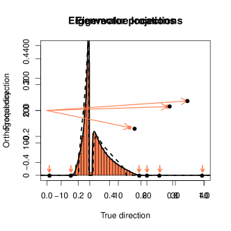
Figure 1. Left: Histogram of sample eigenvalues of the MANOVA estimate for $\Sigma_{1}$ in a one-way layout design, averaged across 1000 simulations, with the four largest and two smallest eigenvalues indicated by red arrows. Six black dots indicate roots of $0=\det T(\lambda)$, predicting the asymptotic locations of these eigenvalues. Overlaid are the densities of the bulk law $\mu_{0}$ (solid black) and of $\mu_{0}$ computed from an isotropic-noise approximation (dashed black). Right: Inner-product of each of three principal sample eigenvectors $(\widehat{v}_{j}:j=1,2,3)$ with the true population eigenvector $e_{j}$ (horizontal axis) and an orthogonal direction $w_{j}$ partially aligned with $\Sigma_{2}$ (vertical axis). Empirical averages across 1000 simulations (red dots/arrows) are overlaid with the predictions of Theorem 2.6 (black dots).

	Predicted (true)			Predicted (isotropic)			Observed
	$\hat{\lambda}$	$\hat{v}^{\top}e_{j}$	$\hat{v}^{\top}w_{j}$	$\hat{\lambda}$	$\hat{v}^{\top}e_{j}$	$\hat{v}^{\top}w_{j}$	$\hat{\lambda}$	$\hat{v}^{\top}e_{j}$	$\hat{v}^{\top}w_{j}$
$\mu_{1}=32$	39.35	0.90	0.07	40.22	0.90	0.07	39.51	0.89	0.07
$\mu_{2}=16$	24.39	0.78	0.03	25.05	0.81	0.03	24.54	0.77	0.03
$\mu_{3}=8$	17.36	0.56	-0.14	17.37	0.71	-0.16	17.26	0.53	-0.13

Table 1. Three principal eigenvalues $\widehat{\lambda}$ and eigenvector inner-products $\widehat{v}_{j}^{\top}e_{j}$ and $\widehat{v}_{j}^{\top}w_{j}$ displayed in Figure 1. Theoretical predictions are computed from Theorems 2.5 and 2.6, using the true noise covariances (left) and an isotropic-noise approximation (middle). Observed values (right) are averaged over 1000 simulations.

Figure 1 and Table 1 illustrate these phenomena in a more complex setting for a balanced one-way layout design, corresponding for example to a twin study with $n=1600$ individuals in $n_{1}=800$ twin pairs, and $p=3200$ traits. We simulate a rank-3 signal component $32e_{1}e_{1}^{\top}+16e_{2}e_{2}^{\top}+8e_{3}e_{3}^{\top}$ in $\Sigma_{1}$ and a rank-2 signal component $32ww^{\top}+64e_{4}e_{4}^{\top}$ in $\Sigma_{2}$, where $w=(e_{1}+e_{2}+e_{3})/\sqrt{3}$, and we sample all remaining eigenvalues of $\Sigma_{1},\Sigma_{2}$ from $\operatorname{Exponential}(1)$. Additional details are provided in Appendix A.2.

Figure 1 displays sample eigenvalues of the MANOVA estimate $\widehat{\Sigma}_{1}$, with numerically computed roots of $0=\det T(\lambda)$. There are 4 positive and 2 negative roots. Of these, the 3rd largest and the smallest (negative) root are attributed to aliasing from $e_{4}$ in $\Sigma_{2}$—their sample eigenvectors are predicted by Theorem 2.6 to be orthogonal to $\{e_{1},e_{2},e_{3}\}$. The 1st, 2nd, and 4th largest roots correspond to the true eigenvalues 32, 16, and 8, each observed with upward bias. For each of the three corresponding sample eigenvectors $\widehat{v}_{j}$, Figure 1 displays its predicted and simulated alignment with the true direction $e_{j}$ and with the orthogonal direction $w_{j}$ obtained by residualizing $e_{j}$ out of $w$. The values of these predicted and simulated eigenvalues and eigenvector alignments are also summarized in Table 1.

3.2. Improved estimation of principal components

The preceding phenomena indicate that the sample eigenvalues and eigenvectors of classical MANOVA estimates for $\Sigma_{1},\ldots,\Sigma_{k}$ are inconsistent in the regime of Assumption 2.2. The estimated eigenvalues in $\widehat{\Sigma}_{r}$ may have upward bias, the estimated eigenvectors may be biased towards eigenvectors of other components $\Sigma_{s}$ for $s\neq r$, and the number of apparent signal principal eigenvectors in $\widehat{\Sigma}_{r}$ may even be incorrect due to aliasing effects from these other components.

The probabilistic results of Theorems 2.5 and 2.6 also suggest a possible route for improved estimation of the principal eigenvalues and eigenvectors: The observed signal eigenvalues of a matrix $\widehat{\Sigma}=Y^{\top}BY$, while inconsistent for the true signal eigenvalues of $\Sigma_{1},\ldots,\Sigma_{k}$, do nonetheless provide some information about these matrices. As indicated by Theorem 2.5, they correspond approximately to roots of the equation $0=\det T(\lambda)$. This matrix $T(\lambda)$ in (11) depends on:

1. The spectra of the $k$ noise covariances $\mathring{\Sigma}_{1},\ldots,\mathring{\Sigma}_{k}$, and the alignments of their eigenvectors across these $k$ different components.

2. The alignments of the rows of $\Gamma$ (the true signal vectors) with these noise covariances $\mathring{\Sigma}_{1},\ldots,\mathring{\Sigma}_{k}$.

3. The sizes of the true signal eigenvalues and the alignments of the signal vectors across these $k$ components, which are related to the magnitudes and inner-products of the rows of $\Gamma$.

Under parametric modeling assumptions for the noise covariance matrices $\mathring{\Sigma}_{1},\ldots,\mathring{\Sigma}_{k}$, the observed outlier eigenvalues $\widehat{\lambda}$ for matrices of the form $\widehat{\Sigma}=Y^{\top}BY$ can yield estimating equations $0=\det T(\widehat{\lambda})$ for the true signal eigenvalues in each component $\Sigma_{1},\ldots,\Sigma_{k}$ (as well as for the cross-component alignments of their corresponding signal eigenvectors). Furthermore, if an estimation matrix $B$ for $\widehat{\Sigma}=Y^{\top}BY$ can be chosen such that the vector $u\in\ker T(\widehat{\lambda})$ is proportional to $\Gamma\,v$, where $\widehat{\lambda}$ is the observed eigenvalue of $\widehat{\Sigma}$ and $v$ is a true signal eigenvector of $\Sigma_{r}$, then Theorem 2.6 indicates that the corresponding sample eigenvector $\widehat{v}$ of $\widehat{\Sigma}$ approximately satisfies $\Gamma\,\widehat{v}\propto\Gamma\,v$, so that $\widehat{v}$ is not asymptotically biased towards the signal direction of a different variance component $\Sigma_{s}$. This debiasing can, for example, lead to asymptotically consistent estimates of linear functionals of this true eigenvector $v$.

These ideas were implemented and analyzed in [FJS18] in the simplest parametric setting where $\mathring{\Sigma}_{r}=\sigma_{r}^{2}\operatorname{Id}$, for each $r=1,\ldots,k$ and some scalar variance parameters $\sigma_{1}^{2},\ldots,\sigma_{k}^{2}$. In this setting, [FJS18] proposed a specific algorithm to solve the estimating equations $0=\det T(\widehat{\lambda})$ arising from a parametric family of matrices $\widehat{\Sigma}=Y^{\top}B(\theta_{1},\ldots,\theta_{k})Y$ to yield estimates of all sufficiently large signal eigenvalues of $\Sigma_{1},\ldots,\Sigma_{k}$. These estimated eigenvalues were shown to be asymptotically consistent in the high-dimensional regime of Assumption 2.2, at a parametric $1/\sqrt{n}$ rate. Furthermore, for each corresponding signal eigenvector $v$, [FJS18] demonstrated how to obtain a specific estimation matrix $B(\theta_{1},\ldots,\theta_{k})$ for which the vector $u\in\ker T(\widehat{\lambda})$ indeed satisfies $u\propto\Gamma\,v$, and thus the algorithm returns a debiased estimate of this true eigenvector $v$. We refer readers to [FJS18] for further details.

When $\mathring{\Sigma}_{1},\ldots,\mathring{\Sigma}_{k}$ are not isotropic, we believe that nonparametric estimation of their spectra and eigenvector alignments may be challenging. However, in certain more parametric contexts—for example when $\mathring{\Sigma}_{1},\ldots,\mathring{\Sigma}_{k}$ capture known autocovariance structure across temporal variables or known genetic correlation structure across quantitative traits, up to a small number of unknown parameters—it may be possible to develop an estimation procedure similar to that of [FJS18], which first estimates these parameters that describe the noise structure in $\mathring{\Sigma}_{1},\ldots,\mathring{\Sigma}_{k}$, and then estimates the principal eigenvalues and eigenvectors of interest, using more general estimating equations that are derived from our results in Theorems 2.5 and 2.6. We leave a more detailed exploration of this possibility to future work.

Isotropic noise is often assumed in practice [PPR06], and our results also provide an understanding of the error that may arise in the original method of [FJS18] due to model misspecification. Figure 1 displays simulated eigenvalue densities $\mu_{0}$ computed using the true matrices $\mathring{\Sigma}_{r}$, which have exponentially decaying spectra, versus using their isotropic noise approximations with $\sigma_{r}^{2}=p^{-1}\operatorname{Tr}\mathring{\Sigma}_{r}$. Table 1 compares the corresponding eigenvalue and eigenvector alignment predictions. We observe that the predictions of Theorems 2.5 and 2.6 for large outliers are very close to those under the isotropic noise approximation. This may also be understood from the calculations in the preceding section for large $\mu_{1},\mu_{2}$, as the dependence of $c_{1},c_{2}$ in (13) on $\mathring{\Sigma}_{1},\mathring{\Sigma}_{2}$ is only through their trace. This suggests that the estimation procedure in [FJS18] may be reasonably accurate for the larger principal eigenvalues and their associated eigenvectors. For eigenvalues closer to the support of the noise spectrum, the predictions of Theorems 2.5 and 2.6 using the true noise covariances $\mathring{\Sigma}_{r}$ are more accurate than those assuming isotropic noise, suggesting that inference for these principal components may be improved by better parametric modeling of the noise structure.

4. Free probability results

Our proofs use the connection between free probability and random matrices. Introducing representations of $U_{r}$, $\alpha_{r}$, and $B$ detailed in Section 5.1, our matrix model $\widehat{\Sigma}$ may be written as

$$\widehat{\Sigma}=W+P,\qquad W=\sum_{r=1}^{k}\sum_{s=1}^{k}H_{r}^{\mathsf{T}}G_{r}^{\mathsf{T}}F_{rs}G_{s}H_{s},$$ (18)

for deterministic matrices $\{H_{1},\ldots,H_{k}\}$ and $\{F_{11},F_{12},\ldots,F_{kk}\}$, independent matrices $\{G_{1},\ldots,G_{k}\}$ with i.i.d. Gaussian entries, and a fixed-rank perturbation $P$ (depending on $G_{1},\ldots,G_{k}$). We study the spectrum of $W$ by introducing an asymptotic approximation

$$w=\sum_{r=1}^{k}\sum_{s=1}^{k}h_{r}^{*}g_{r}^{*}f_{rs}g_{s}h_{s},$$

where $h_{r},g_{r},f_{rs}$ belong to a von Neumann algebra and are conditionally free (i.e. free with amalgamation) over a diagonal subalgebra [BG09]. This method was also used in [FJ19] to derive the fixed-point equations (6–8) in Theorem 2.3.

Our analysis develops several new tools and results in free probability theory. In this section, we state these results independent of the specific model (1), as they are of general interest for analyzing structured random matrices in other applications. We defer proofs to Appendices B, C, and D.

4.1. Augmented Cauchy and $R$-transforms

We call $(\mathcal{A},\tau)$ a von Neumann probability space ($W^{*}$-probability space) if $\mathcal{A}$ is a von Neumann algebra and $\tau:\mathcal{A}\to\mathbb{C}$ a positive, faithful, normal trace. For a von Neumann subalgebra $\mathcal{B}\subset\mathcal{A}$, we denote by

$$\tau^{\mathcal{B}}:\mathcal{A}\to\mathcal{B}$$

the (unique) conditional expectation satisfying $\tau(\tau^{\mathcal{B}}(a))=\tau(a)$.

We review the following definitions of $\mathcal{B}$-valued Cauchy- and $\mathcal{R}$-transforms: For each $l\geq 1$, let $\text{NC}(l)$ be the space of non-crossing partitions of $1,\ldots,l$. For $\pi\in\text{NC}(l)$, denote by $\kappa_{\pi}^{\mathcal{B}}(a_{1},\ldots,a_{l})$ the non-crossing cumulant corresponding to $\pi$. These satisfy the moment-cumulant relations

$$\tau^{\mathcal{B}}(a_{1}a_{2}\ldots a_{l})=\sum_{\pi\in\text{NC}(l)}\kappa_{\pi}^{\mathcal{B}}(a_{1},a_{2},\ldots,a_{l}).$$ (19)

Define the $\mathcal{B}$-valued Cauchy- and $\mathcal{R}$-transform of $a\in\mathcal{A}$ by

$$G_{a}^{\mathcal{B}}(b)=\tau^{\mathcal{B}}((b-a)^{-1})=\sum_{l\geq 0}b^{-1}(ab^{-1})^{l},\qquad\mathcal{R}_{a}^{\mathcal{B}}(b)=\sum_{l\geq 1}\kappa_{l}^{\mathcal{B}}(a,ba,\ldots,ba),$$

the former for all invertible $b\in\mathcal{B}$ with $\|b^{-1}\|$ sufficiently small and the latter for all $b\in\mathcal{B}$ with $\|b\|$ sufficiently small. The moment-cumulant relations (19) yield the identity

$$G_{a}^{\mathcal{B}}(b)=(b-\mathcal{R}_{a}^{\mathcal{B}}(G_{a}^{\mathcal{B}}(b)))^{-1}$$ (20)

for invertible $b\in\mathcal{B}$ with $\|b^{-1}\|$ sufficiently small. We refer the reader to [MS17, Chapter 9] for additional background and details.

For our computations in Section 5, we will make use of the following “left-augmented” Cauchy- and $R$-transforms, defined for $a_{1},a\in\mathcal{A}$ and $b\in\mathcal{B}$ by the mixed moments and mixed cumulants

$$G^{\mathcal{B}}_{a_{1},a}(b) =\tau^{\mathcal{B}}\Big{(}a_{1}(b-a)^{-1}\Big{)}=\sum_{l\geq 0}\tau^{\mathcal{B}}(a_{1}b^{-1}(ab^{-1})^{l}),$$ (21)

$$R^{\mathcal{B}}_{a_{1},a}(b) =\sum_{l\geq 1}\kappa_{l}^{\mathcal{B}}(a_{1},ba,\ldots,ba).$$ (22)

The following identity is then also a consequence of (19), and we provide a short proof in Appendix B.

Lemma 4.1.

For $a_{1},a\in\mathcal{A}$ and all invertible $b\in\mathcal{B}$ with $\|b^{-1}\|$ sufficiently small,

$$G^{\mathcal{B}}_{a_{1},a}(b)=R^{\mathcal{B}}_{a_{1},a}(G^{\mathcal{B}}_{a}(b))G^{\mathcal{B}}_{a}(b).$$ (23)

4.2. Strong asymptotic freeness of GOE and deterministic matrices

We establish a strong asymptotic freeness result for GOE and deterministic matrices, which is the real analogue of the GUE result in [Mal12]. The proof is provided in Appendix C.

Fix integers $p,q\geq 0$. Let $X_{1},\ldots,X_{p}\in\mathbb{R}^{N\times N}$ be independent GOE matrices, with diagonal entries distributed as $\mathcal{N}(0,2/N)$ and off-diagonal entries as $\mathcal{N}(0,1/N)$. Let $Y_{1},\ldots,Y_{q}\in\mathbb{C}^{N\times N}$ be deterministic matrices. Denote $\mathbf{X}_{N}=\left(X_{1},\ldots,X_{p}\right)$ and $\mathbf{Y}_{N}=\left(Y_{1},\ldots,Y_{q}\right)$. Let $\operatorname{tr}_{N}=N^{-1}\operatorname{Tr}$ be the normalized matrix trace on $\mathbb{C}^{N\times N}$.

Consider an $N$-dependent von Neumann probability space $(\mathcal{A}_{N},\tau_{N})$. Suppose $\mathcal{A}_{N}$ contains $x_{1},\ldots,x_{p}$ and $Y_{1},\ldots,Y_{q}$, where $x_{1},\ldots,x_{p}$ are free semicircular elements also free of $Y_{1},\ldots,Y_{q}$, and $\tau_{N}\equiv\operatorname{tr}_{N}$ restricted to the von Neumann subalgebra $\langle Y_{1},\ldots,Y_{q}\rangle$. Denote $\mathbf{x}=(x_{1},\ldots,x_{p})$.

Theorem 4.2.

Suppose $\|Y_{j}\|\leq C$ for all $j=1,\ldots,q$ and a constant $C>0$. Then for any fixed non-commutative self-adjoint $*$-polynomial $Q$ in $p+q$ variables, and any constant $\delta>0$, almost surely for all large $N$,

$$\operatorname{spec}(Q(\mathbf{X}_{N},\mathbf{Y}_{N}))\subset\operatorname{spec}(Q(\mathbf{x},\mathbf{Y}_{N}))_{\delta}.$$ (24)

Here, $\operatorname{spec}(Q(\mathbf{X}_{N},\mathbf{Y}_{N}))$ are the eigenvalues of the self-adjoint random matrix $Q(\mathbf{X}_{N},\mathbf{Y}_{N})\in\mathbb{C}^{N\times N}$, and $\operatorname{spec}(Q(\mathbf{x},\mathbf{Y}_{N}))_{\delta}$ is the $\delta$-neighborhood of the spectrum of the operator $Q(\mathbf{x},\mathbf{Y}_{N})\in\mathcal{A}_{N}$.

For our application, we will apply strong asymptotic freeness directly in the above form. However, we may also obtain as a corollary the following more usual statement, by the arguments of [Mal12, Section 7].

Theorem 4.3.

Let $\mathbf{x}=(x_{1},\ldots,x_{p})$ and $\mathbf{y}=(y_{1},\ldots,y_{q})$ be elements of a fixed von Neumann probability space $(\mathcal{A},\tau)$, such that $x_{1},\ldots,x_{p}$ are free semicircular elements also free from $\mathbf{y}$. Assume that almost surely as $N\to\infty$, for any fixed self-adjoint $*$-polynomial $P$ in $q$ variables,

$$\operatorname{tr}_{N}[P(\mathbf{Y}_{N})]\rightarrow\tau(P(\mathbf{y}))\quad\text{and}\quad\|P(\mathbf{Y}_{N})\|\rightarrow\|P(\mathbf{y})\|.$$

Then, almost surely for any self-adjoint $*$-polynomial $Q$ in $p+q$ variables,

$$\operatorname{tr}_{N}[Q(\mathbf{X}_{N},\mathbf{Y}_{N})]\rightarrow\tau(Q(\mathbf{x},\mathbf{y}))\quad\text{and}\quad\|Q(\mathbf{X}_{N},\mathbf{Y}_{N})\|\rightarrow\|Q(\mathbf{x},\mathbf{y})\|.$$ (25)

4.3. Resolvent approximation using free deterministic equivalents

We also establish a method of approximating bilinear forms in resolvents using the free deterministic equivalent framework of [SV12].

Fix integers $p,q\geq 0$. We study the resolvent $R(z)$ of a random matrix

$$W=Q(H_{1},\ldots,H_{p},B_{1},\ldots,B_{q})\in\mathbb{C}^{N\times N},$$ (26)

where $Q$ is any self-adjoint $*$-polynomial, $H_{1},\ldots,H_{p}$ are deterministic, and $B_{1},\ldots,B_{q}$ are random matrices orthogonally invariant in law. For spectral arguments $z$ with constant separation from $\operatorname{spec}(W)$, and any deterministic unit vectors $u,v\in\mathbb{C}^{N}$, we will show an approximation

$$u^{*}R(z)v\approx u^{*}R_{0}(z)v,$$

where $R_{0}(z)$ is a deterministic matrix defined by a free deterministic equivalent model.

We consider a setup that will allow us to study rectangular matrices, following [BG09]: Let $\mathcal{A}_{1}=\mathbb{C}^{N\times N}$ and $\tau_{1}=N^{-1}\operatorname{Tr}$. Fix $k\geq 1$, let $N=N_{1}+\ldots+N_{k}$, and consider the associated $k\times k$ block decomposition of $\mathcal{A}_{1}$. Define mutually orthogonal projections $P_{1},\ldots,P_{k}\in\mathcal{A}_{1}$ by

$$P_{r}=\operatorname{diag}(0,\ldots,0,\operatorname{Id}_{N_{r}},0,\ldots,0)$$

with $\operatorname{Id}_{N_{r}}$ in the $r$th diagonal block. Then $(\mathcal{A}_{1},\tau_{1},P_{1},\ldots,P_{k})$ is a rectangular probability space in the sense of [BG09]. Define the subalgebra $\mathcal{D}\subset\mathcal{A}_{1}$ generated by $P_{1},\ldots,P_{k}$, given explicitly by

$$\mathcal{D}=\{z_{1}P_{1}+\ldots+z_{k}P_{k}:z_{1},\ldots,z_{k}\in\mathbb{C}\}.$$

Define also the space of block-diagonal orthogonal matrices

$$\mathcal{O}=\{\operatorname{diag}(O_{1},\ldots,O_{k}):O_{r}\in\mathbb{R}^{N_{r}\times N_{r}},\,O_{r}^{\mathsf{T}}O_{r}=\operatorname{Id}\text{ for each }r\}.$$

Consider $H_{1},\ldots,H_{p},B_{1},\ldots,B_{q}\in\mathcal{A}_{1}$, where $H_{1},\ldots,H_{p}$ are deterministic, and $(B_{1},\ldots,B_{q})$ is random and equal in joint law to $(OB_{1}O^{\mathsf{T}},\ldots,OB_{q}O^{\mathsf{T}})$ for all $O\in\mathcal{O}$. For a self-adjoint $*$-polynomial $Q$ in $p+q$ arguments with coefficients in $\mathcal{D}$, define $W$ by (26), and define its resolvent

$$R(z)=(W-z\operatorname{Id})^{-1}.$$

To define the approximation $R_{0}(z)$, we construct a free deterministic equivalent model: Let $(\mathcal{A}_{2},\tau_{2})$ be a second von Neumann probability space, where $\mathcal{D}\subset\mathcal{A}_{2}$ and $\tau_{1}\equiv\tau_{2}$ restricted to $\mathcal{D}$. Let $\mathcal{A}_{2}$ have elements $b_{1},\ldots,b_{q}$ satisfying

$$N^{-1}\operatorname{Tr}\Big{(}P(B_{1},\ldots,B_{q})\Big{)}-\tau_{2}\Big{(}P(b_{1},\ldots,b_{q})\Big{)}\to 0$$ (27)

almost surely as $N\to\infty$, for any fixed $*$-polynomial $P$ with coefficients in $\mathcal{D}$. Define the von Neumann amalgamated free product over $\mathcal{D}$,

$$(\mathcal{A},\tau)=(\mathcal{A}_{1},\tau_{1})*_{\mathcal{D}}(\mathcal{A}_{2},\tau_{2}),$$

so that $(H_{1},\ldots,H_{p})$ is free of $(b_{1},\ldots,b_{q})$ with amalgamation over $\mathcal{D}$. Define the free deterministic equivalent approximation to $W$ by

$$w=Q(H_{1},\ldots,H_{p},b_{1},\ldots,b_{q})\in\mathcal{A}.$$

Finally, let $\mathcal{H}=\langle H_{1},\ldots,H_{p},\mathcal{D}\rangle$ be the generated von Neumann subalgebra of $\mathcal{A}$, and let $\tau^{\mathcal{H}}:\mathcal{A}\to\mathcal{H}$ be the conditional expectation onto $\mathcal{H}$ that satisfies $\tau(\tau^{\mathcal{H}}(a))=\tau(a)$. Importantly, note that for any $a\in\mathcal{A}$,

$$\tau^{\mathcal{H}}(a)\in\mathcal{H}\subset\mathcal{A}_{1}\equiv\mathbb{C}^{N\times N},$$

so that $\tau^{\mathcal{H}}(a)$ is an $N\times N$ matrix. We define the free deterministic approximation $R_{0}(z)$ of $R(z)$ by

$$R_{0}(z)=\tau^{\mathcal{H}}((w-z)^{-1}).$$ (28)

We now state our approximation result, whose proof is in Appendix D.

Theorem 4.4 (Resolvent approximation).

For some constants $C,c>0$, suppose $c<N_{r}/N<C$, $\|H_{i}\|<C$, and $\|B_{j}\|<C$ for all $r,i,j$, almost surely for all large $N$. Fix any constant $\delta>0$ and set

$$\mathbb{D}=\{z\in\mathbb{C}:\operatorname{dist}(z,\operatorname{spec}(w))\geq\delta\text{ and }\operatorname{dist}(z,\operatorname{spec}(W))\geq\delta\}.$$

Then for any (sequence of) deterministic unit vectors $u,v\in\mathbb{C}^{N}$, almost surely as $N\to\infty$,

$$\sup_{z\in\mathbb{D}}|u^{*}R(z)v-u^{*}R_{0}(z)v|\to 0.$$ (29)

Taking $k=1$ yields a result for square orthogonally invariant matrices, where $(\mathcal{A},\tau)$ is the von Neumann free product over $\mathcal{D}\equiv\mathbb{C}$. We consider $k\geq 2$ to encompass applications with rectangular matrices, where each $H_{i},B_{j}$ typically has a single off-diagonal block which is non-zero. We are then interested in $*$-polynomials $Q$ that are $(1,1)$-simple, i.e. $W$ and $w$ satisfy

$$W=P_{1}WP_{1},\qquad w=P_{1}wP_{1}.$$

Denote by $W_{11}\in\mathbb{C}^{N_{1}\times N_{1}}$ the $(1,1)$-block of $W$. Corresponding to $\mathbb{C}^{N_{1}\times N_{1}}$ is a “compressed algebra” $\mathcal{A}^{c}=\{P_{1}aP_{1}:a\in\mathcal{A}\}$ with unit $P_{1}$ [SV12]. Denote by $w_{11}\in\mathcal{A}^{c}$ and $\operatorname{spec}(w_{11})$ the element $w$ and its spectrum, viewed as a self-adjoint operator in $\mathcal{A}^{c}$. We then have the following corollary.

Corollary 4.5.

In the setting of Theorem 4.4, suppose in addition that $W=P_{1}WP_{1}$ and $w=P_{1}wP_{1}$, and let $W_{11}$ and $w_{11}$ be as above. Let $(R_{0}(z))_{11}\in\mathbb{C}^{N_{1}\times N_{1}}$ be the $(1,1)$-block of $R_{0}(z)=\tau^{\mathcal{H}}((w-z)^{-1})$, and set

$$\mathbb{D}_{1}=\{z\in\mathbb{C}:\operatorname{dist}(z,\operatorname{spec}(w_{11}))\geq\delta\text{ and }\operatorname{dist}(z,\operatorname{spec}(W_{11}))\geq\delta\}.$$

Then for any (sequence of) deterministic unit vectors $u_{1},v_{1}\in\mathbb{C}^{N_{1}}$, almost surely as $N\to\infty$,

$$\sup_{z\in\mathbb{D}_{1}}|u_{1}^{*}(W_{11}-z\operatorname{Id})^{-1}v_{1}-u_{1}^{*}(R_{0}(z))_{11}v_{1}|\to 0.$$ (30)

5. Analysis of the linear mixed model

In this section, we give a high-level outline of the proofs of Theorems 2.5 and 2.6, which follow the perturbative approach of [BGN11]. We present the main steps of the computations, deferring technical details to Appendix E.

We assume implicitly throughout that Assumptions 2.1 and 2.2 hold. We denote by $C,c>0$ constants which may change from instance to instance. We fix a constant $\delta>0$, and define

$$U_{\delta}=\{z\in\mathbb{C}:\operatorname{dist}(z,\operatorname{supp}(\mu_{0}))>\delta\}.$$

We denote $\|X\|_{\infty}=\max_{i,j}|X_{i,j}|$. For $n$-dependent matrices $X_{1}(z),X_{2}(z)$ of the same (bounded) dimension, we write

$$X_{1}(z)\sim X_{2}(z)$$

if almost surely as $n\to\infty$, we have

$$\sup_{z\in U_{\delta}}\|X_{1}(z)-X_{2}(z)\|_{\infty}\to 0.$$

5.1. Model and deterministic equivalent measure

We first clarify the form of $\widehat{\Sigma}$ and the free probability interpretation of the measure $\mu_{0}$. Introducing $\Gamma_{r}\in\mathbb{R}^{\ell_{r}\times p}$ as in (2), and defining

$$\Xi_{r}=\frac{1}{\sqrt{n_{r}}}(\xi_{ij}^{(r)})_{i,j}\in\mathbb{R}^{n_{r}\times\ell_{r}},\qquad E_{r}=\begin{pmatrix}-&\varepsilon_{1}^{(r)}&-\\ &\vdots&\\ -&\varepsilon_{n}^{(r)}&-\end{pmatrix}\in\mathbb{R}^{n_{r}\times p},$$

the random effect matrix $\alpha_{r}$ is written concisely as

$$\alpha_{r}=\sqrt{n_{r}}\,\Xi_{r}\Gamma_{r}+E_{r}.$$ (31)

Write further

$$E_{r}=\sqrt{n_{r}}\,G_{r}H_{r},$$ (32)

where $G_{r}\in\mathbb{R}^{n_{r}\times p}$ has i.i.d. $\mathcal{N}(0,1/n_{r})$ entries and $H_{r}=\mathring{\Sigma}^{1/2}\in\mathbb{R}^{p\times p}$. Then, when $\ell_{r}=0$ and $\alpha_{r}=E_{r}$ for all $r$, we obtain

$$\widehat{\Sigma}=W\equiv\sum_{r,s=1}^{k}H_{r}^{\mathsf{T}}G_{r}^{\mathsf{T}}F_{rs}G_{s}H_{s},$$

where $\{F_{rs}:r,s=1,\ldots,k\}$ are defined in (5). More generally, we have

$$\widehat{\Sigma}=\sum_{r,s=1}^{k}(\Xi_{r}\Gamma_{r}+G_{r}H_{r})^{\mathsf{T}}F_{rs}(\Xi_{s}\Gamma_{s}+G_{s}H_{s})=W+P$$ (33)

for $W$ as above, and for the low-rank perturbation

$$P=\sum_{r,s=1}^{k}\Big{(}\Gamma_{r}^{\mathsf{T}}\Xi_{r}^{\mathsf{T}}F_{rs}G_{s}H_{s}+H_{r}^{\mathsf{T}}G_{r}^{\mathsf{T}}F_{rs}\Xi_{s}\Gamma_{s}+\Gamma_{r}^{\mathsf{T}}\Xi_{r}^{\mathsf{T}}F_{rs}\Xi_{s}\Gamma_{s}\Big{)}.$$ (34)

The proof of Theorem 2.3 in [FJ19] used a free probability approach. As the matrices $G_{r}$ and $F_{rs}$ in this model are rectangular, asymptotic freeness was formally expressed using the ideas of [BG09], by embedding these matrices in a larger square matrix, and establishing asymptotic freeness with amalgamation over a subalgebra generated by block-identity matrices along the diagonal.

More specifically, the proof in [FJ19, Section 4] illustrates that $\mu_{0}$ is a spectral measure in the following model: Set $N=(k+1)p+n_{1}+\ldots+n_{k}$. Embed $\{F_{rs},G_{r},H_{r}:r,s=1,\ldots,k\}$ into $\mathbb{C}^{N\times N}$ by zero-padding, in the following blocks of the $(2k+1)\times(2k+1)$ block decomposition for $\mathbb{C}^{N}=\mathbb{C}^{p}\oplus\cdots\oplus\mathbb{C}^{p}\oplus\mathbb{C}^{n_{1}}\cdots\oplus\mathbb{C}^{n_{k}}$:

$$\begin{pmatrix}&H_{1}^{*}&\cdots&H_{k}^{*}&&&\\ H_{1}&&&&G_{1}^{*}&&\\ \vdots&&&&&\ddots&\\ H_{k}&&&&&&G_{k}^{*}\\ &G_{1}&&&F_{11}&\cdots&F_{1k}\\ &&\ddots&&\vdots&\ddots&\vdots\\ &&&G_{k}&F_{k1}&\cdots&F_{kk}\end{pmatrix}$$ (35)

Denote by $\tilde{F}_{rs}$, $\tilde{G}_{r}$, and $\tilde{H}_{r}\in\mathbb{C}^{N\times N}$ these embedded matrices. Consider the mutually orthogonal projections

$$P_{0}=\operatorname{diag}(\operatorname{Id}_{p},0,\ldots,0),\quad\ldots,\quad P_{2k}=\operatorname{diag}(0,\ldots,0,\operatorname{Id}_{n_{k}})$$

corresponding to the $2k+1$ diagonal blocks of $\mathbb{C}^{N\times N}$. Then the block structure of this embedding induces an asymptotic freeness of the families $\{F_{rs}\}$, $\{H_{r}\}$, and individual matrices $G_{1},\ldots,G_{k}$ with amalgamation over the subalgebra generated by these projections $\{P_{0},\ldots,P_{2k}\}$.

Let $(\mathcal{A},\tau)$ be a von Neumann probability space containing mutually orthogonal projections $p_{0},p_{1},\ldots,p_{2k}$ which analogously satisfy $\tau(p_{0})=\ldots=\tau(p_{k})=p/N$ and $\tau(p_{k+r})=n_{r}/N$ for each $r=1,\ldots,k$. Let $(\mathcal{A},\tau)$ also contain $\{f_{rs},g_{r},h_{r}:r,s=1,\ldots,k\}$ such that

1. $p_{k+r}f_{rs}p_{k+s}$, $p_{k+r}g_{r}p_{r}=g_{r}$, and $p_{r}h_{r}p_{0}=h_{r}$.

2. For any non-commutative $*$-polynomial $Q$ of $k$ variables,

   $$\tau(Q(h_{1},\ldots,h_{k}))=N^{-1}\operatorname{Tr}Q(\tilde{H}_{1},\ldots,\tilde{H}_{k}).$$

   Similarly, for any non-commutative $*$-polynomial $Q$ of $k^{2}$ variables,

   $$\tau(Q(f_{11},f_{12},\ldots,f_{kk}))=N^{-1}\operatorname{Tr}Q(\tilde{F}_{11},\tilde{F}_{12},\ldots,\tilde{F}_{kk}).$$

3. For each $r\in\{1,\ldots,k\}$ and $l\geq 0$,

   $$\frac{N}{p}\tau((g_{r}^{*}g_{r})^{l})=\int x^{l}\nu_{p/n_{r}}(dx)$$

   where $\nu$ is the Marcenko-Pastur law with parameter $p/n_{r}$.

4. The families $\{f_{rs}:r,s=1,\ldots,k\}$, $\{h_{r}:r=1,\ldots,k\}$, and individual elements $g_{1},\ldots,g_{k}$ are free with amalgamation over the von Neumann subalgebra $\mathcal{D}=\langle p_{0},\ldots,p_{2k}\rangle$.

Define a free deterministic equivalent for $W$ by

$$w=\sum_{r,s=1}^{k}h_{r}^{*}g_{r}^{*}f_{rs}g_{s}h_{s}.$$ (36)

Only the $(0,0)$-block of $w$ is non-zero—this corresponds to $W$ belonging to the $(0,0)$ block in the embedded space (35). Thus $w$ is an element of the compressed algebra $\mathcal{A}^{c}=\{a\in\mathcal{A}:a=p_{0}ap_{0}\}$, which has unit $p_{0}$ and trace $\tau^{c}(a)=(N/p)\tau(p_{0}ap_{0})$. The analysis of [FJ19, Section 4] shows that the law $\mu_{0}$ in Theorem 2.3 is the $\tau^{c}$-distribution of $w$. This means that for any continuous function $f:\mathbb{R}\to\mathbb{C}$, we have

$$\int f(x)d\mu_{0}(x)=\tau^{c}(f(w))$$

where $f(w)$ is defined by the functional calculus on $\mathcal{A}^{c}$. Since $\tau$ is a faithful trace, so is $\tau^{c}$ as a trace on $\mathcal{A}^{c}$, and thus (cf. [NS06, Prop. 3.13 and 3.15])

$$\operatorname{supp}(\mu_{0})=\operatorname{spec}(w)$$ (37)

where $\operatorname{spec}(w)$ is the spectrum of $w$ as an element of $\mathcal{A}^{c}$.

5.2. Master equation

Following [BGN11], we first establish a “master equation” characterizing outlier eigenvalues of $\widehat{\Sigma}$.

Recall the form (33) for $\widehat{\Sigma}$. Letting $\ell$ be the rank of $\Gamma$ (so $\ell\leq\ell_{+}$), write

$$\Gamma=\widetilde{\Gamma}Q^{\mathsf{T}}$$

where $Q\in\mathbb{R}^{p\times\ell}$ contains the right singular vectors of $\Gamma$. We have $Q^{\mathsf{T}}Q=\operatorname{Id}_{\ell}$ and $\|\widetilde{\Gamma}\|\leq C$. Denote the resolvent of $W$ by

$$R(z)=(W-z\operatorname{Id})^{-1}.$$

Define the block-diagonal matrices

$$\Xi=\left[\begin{matrix}\Xi_{1}&&&\\ &\Xi_{2}&&\\ &&\ddots&\\ &&&\Xi_{k}\end{matrix}\right]\in\mathbb{R}^{n_{+}\times\ell_{+}},\quad G=\left[\begin{matrix}G_{1}&&&\\ &G_{2}&&\\ &&\ddots&\\ &&&G_{k}\end{matrix}\right]\in\mathbb{R}^{n_{+}\times kp}.$$

Finally, define $H\in\mathbb{R}^{kp\times p}$ as the vertical stacking of $\{H_{r}\}_{r=1}^{k}$, and set

$$S(z)=\Xi^{\mathsf{T}}FGHR(z)Q.$$

In Appendix E.2, we write the low-rank perturbation matrix $P$ in (34) as $P=P_{1}P_{2}$ for two rectangular matrices $P_{1}$ and $P_{2}$. We then apply the identity $\det(\operatorname{Id}+R(z)P_{1}P_{2})=\det(\operatorname{Id}+P_{2}R(z)P_{1})$ to obtain the following result.

Lemma 5.1.

The eigenvalues of $\widehat{\Sigma}$ which are not eigenvalues of $W$ are the roots of $\det\widehat{K}(z)=0$, where

$$\widehat{K}(z)=\operatorname{Id}+\left[\begin{matrix}S(z)\cdot\widetilde{\Gamma}^{\mathsf{T}}&\Xi^{\mathsf{T}}FGHR(z)H^{\mathsf{T}}G^{\mathsf{T}}F\Xi\cdot\widetilde{\Gamma}+S(z)\cdot\widetilde{\Gamma}^{\mathsf{T}}\Xi^{\mathsf{T}}F\Xi\widetilde{\Gamma}\\ Q^{\mathsf{T}}R(z)Q\cdot\widetilde{\Gamma}^{\mathsf{T}}&S(z)^{\mathsf{T}}\cdot\widetilde{\Gamma}+Q^{\mathsf{T}}R(z)Q\cdot\widetilde{\Gamma}^{\mathsf{T}}\Xi^{\mathsf{T}}F\Xi\widetilde{\Gamma}\end{matrix}\right].$$ (38)

Denote the four blocks of this matrix as $\widehat{K}_{11},\widehat{K}_{12},\widehat{K}_{21},\widehat{K}_{22}$. When $\widehat{K}_{11}$ is invertible, the condition $\det\widehat{K}(z)=0$ is equivalent to $\det\widehat{T}(z)=0$ for the Schur complement

$$\widehat{T}(z)=\widehat{K}_{22}(z)-\widehat{K}_{21}(z)\widehat{K}_{11}(z)^{-1}\widehat{K}_{12}(z).$$ (39)

Observe that each matrix $\Xi^{\top}(\ldots)\Xi$ in the definition of $\widehat{K}$ has bounded dimension $\ell_{+}\times\ell_{+}$, each matrix $\Xi^{\top}(\ldots)Q$ has bounded dimension $\ell_{+}\times\ell$, and $\Xi$ is independent of $G$ and $R(z)$. Then, conditioning on $G$ and $R(z)$ and applying concentration inequalities for linear and bilinear forms in $\Xi$, we obtain that $\widehat{T}(z)$ is approximated by a matrix

$$\widecheck{T}(z)=\operatorname{Id}+Q^{\mathsf{T}}R(z)Q\cdot\widetilde{\Gamma}^{\mathsf{T}}\left(\sum_{r=1}^{k}n_{r}^{-1}\operatorname{Tr}_{r}[F-FGHR(z)H^{\mathsf{T}}G^{\mathsf{T}}F]\operatorname{Id}_{\ell_{r}}\right)\widetilde{\Gamma}.$$ (40)

This is formalized in the following result, proven in Appendix E.2.

Lemma 5.2.

We have that $S(z)\sim 0$, $\widehat{K}_{11}(z)\sim\operatorname{Id}_{\ell_{+}}$, and $\widehat{T}(z)\sim\widecheck{T}(z)$.

The outlier eigenvalues of $\widehat{\Sigma}$ will be approximate roots of $0=\det\widecheck{T}(z)$, where this matrix $\widecheck{T}(z)$ no longer depends on the randomness in $\Xi$.

5.3. Approximation by deterministic equivalents

The main step of the proof is to approximate the $G$- and $R(z)$-dependent terms appearing in (40) by deterministic quantities. We do this using a free deterministic equivalent approach. Define

$$\widetilde{T}(z)=\operatorname{Id}+Q^{\mathsf{T}}(z\operatorname{Id}+\mathbf{b}\cdot\mathring{\Sigma})^{-1}Q\cdot\widetilde{\Gamma}^{\mathsf{T}}\operatorname{diag}_{\ell}(\mathbf{b})\widetilde{\Gamma},$$

with notation as in Theorem 2.5. Our goal is to show the following lemma.

Lemma 5.3.

We have $\widecheck{T}(z)\sim\widetilde{T}(z)$.

This requires approximating the two terms in $\widecheck{T}$ by those in $\widetilde{T}$. For approximating the first term, as perhaps can be guessed from the form of the Stieltjes transform (8), the matrix $-(z\operatorname{Id}+\mathbf{b}\cdot\mathring{\Sigma})^{-1}$ is a deterministic equivalent for the resolvent $R(z)$. We verify this in the following result, using the resolvent approximation techniques in Section 4.3 and Theorem 4.4.

Proposition 5.4.

We have $Q^{\mathsf{T}}R(z)Q\sim-Q^{\mathsf{T}}(z\operatorname{Id}+\mathbf{b}\cdot\mathring{\Sigma})^{-1}Q$.

Proof.

The von Neumann probability space $(\mathcal{A},\tau)$ in Section 5.1 may be constructed as follows: Let $(\mathcal{A}_{1},\tau_{1})=(\mathbb{C}^{N\times N},N^{-1}\operatorname{Tr})$, containing the embeddings of the matrices $H_{1},\ldots,H_{k}$ and $P_{0},\ldots,P_{2k}$. Denote these elements of $\mathcal{A}_{1}$ also by $h_{r}$ and $p_{r}$. Construct a von Neumann probability space $(\mathcal{A}_{2},\tau_{2})$ also containing $p_{0},\ldots,p_{2k}$ and elements $\{f_{rs},g_{r}:r,s=1,\ldots,k\}$ satisfying all required conditions on their joint law under $\tau_{2}$. Let $(\mathcal{A},\tau)$ be the von Neumann amalgamated free product over $\langle p_{0},\ldots,p_{2k}\rangle$.

Let $w=\sum_{r,s}h_{r}^{*}g_{r}^{*}f_{rs}g_{s}h_{s}\in\mathcal{A}$. By Corollary 4.5 applied to each pair of columns of $Q$, we find that

$$Q^{\mathsf{T}}R(z)Q\sim Q^{\mathsf{T}}P_{0}\tau^{\mathcal{H}}((w-z)^{-1})P_{0}Q$$

where $P_{0}\tau^{\mathcal{H}}((w-z)^{-1})P_{0}$ is identified with its $(0,0)$-block as an element of $\mathbb{C}^{p\times p}$. This $\tau^{\mathcal{H}}$ trace was computed in [FJ19, Equation (4.12)] to be

$$\tau^{\mathcal{H}}\Big{(}(w-z)^{-1}\Big{)}=-\left(z+\sum_{r=1}^{k}h_{r}^{*}h_{r}b_{r}(z)\right)^{-1},$$

using the identification $\beta_{r}(z)=-b_{r}(z)$ at the conclusion of the proof of [FJ19, Lemma 4.4]. The $(0,0)$-block of this matrix is exactly

$$-\left(z+\sum_{r=1}^{k}H_{r}^{\mathsf{T}}H_{r}b_{r}(z)\right)^{-1}=-(z+\mathbf{b}\cdot\mathring{\Sigma})^{-1}.\qquad\qed$$

Lemma 5.3 now follows by applying Proposition 5.4 and the following approximation for the second term of $\widecheck{T}(z)$.

Proposition 5.5.

For each $t\in\{1,\ldots,k\}$, we have

$$n_{t}^{-1}\operatorname{Tr}_{t}[F-FGHR(z)H^{\mathsf{T}}G^{\mathsf{T}}F]\sim-b_{t}(z).$$

In the remainder of this section, we prove Proposition 5.5. We apply a computation using the augmented Cauchy- and $\mathcal{R}$-transforms of Section 4.1. In the von Neumann probability space $(\mathcal{A},\tau)$ of Section 5.1, let $\mathcal{H}=\langle h_{1},\ldots,h_{k}\rangle$, $\mathcal{G}=\langle g_{1},\ldots,g_{k}\rangle$, $\mathcal{F}=\langle f_{11},f_{12},\ldots,f_{kk}\rangle$ and $\mathcal{D}=\langle p_{0},\ldots,p_{2k}\rangle$ be the generated von Neumann subalgebras of $\mathcal{A}$. Define the elements

$$w=\sum_{r,s=1}^{k}h_{r}^{*}g_{r}^{*}f_{rs}g_{s}h_{s}\qquad v=\sum_{r,s=1}^{k}g_{r}^{*}f_{rs}g_{s}\qquad u=\sum_{r,s=1}^{k}f_{rs}.$$ (41)

For any $r,s,t\in\{1,\ldots,k\}$ define

$$a_{rts}=h_{r}^{*}g_{r}^{*}f_{rt}f_{ts}g_{s}h_{s}\qquad b_{rts}=g_{r}^{*}f_{rt}f_{ts}g_{s}\qquad c_{rts}=f_{rt}f_{ts}.$$

Our goal is to compute

$$\sum_{r,s=1}^{k}\tau(f_{ts}g_{s}h_{s}(w-z)^{-1}h_{r}^{*}g_{r}^{*}f_{rt})=\sum_{s,t=1}^{k}\tau(a_{rts}(w-z)^{-1}),$$

which is the free approximation for $\operatorname{Tr}_{t}FGHR(z)H^{\mathsf{T}}G^{\mathsf{T}}F$.

For $a\in\mathcal{A}$ and $h\in\mathcal{H}$, define the $\mathcal{H}$-valued conditional expectation $\tau^{\mathcal{H}}(a)$, Cauchy-transform $G^{\mathcal{H}}_{a}(h)$, and $\mathcal{R}$-transform $\mathcal{R}^{\mathcal{H}}_{a}(h)$, and similarly for $\mathcal{G}$ and $\mathcal{D}$. For each $i\in\{0,\ldots,2k\}$, denote

$$\tau_{i}(a)=\tau(p_{i})^{-1}\tau(p_{i}ap_{i})$$

and note that $\tau^{\mathcal{D}}(a)=\sum_{i}\tau_{i}(a)p_{i}$. For a sufficiently large constant $C>0$, define

$$\mathbb{D}=\{z\in\mathbb{C}:|z|>C\}.$$

We define the following analytic functions $\{\alpha_{i}\}_{i=0}^{2k}$, $\{\beta_{i}\}_{i=0}^{2k}$, $\{d_{i}\}_{i=0}^{2k}$, $\{\gamma_{j}\}_{j=0}^{2k}$, $\{\delta_{j}\}_{j=0}^{2k}$, and $\{e_{j}\}_{j=0}^{2k}$ on $\mathbb{D}$, also used in [FJ19]: For $i=1,\ldots,k$, define

$$\alpha_{i}=\tau_{i}(h_{i}G^{\mathcal{H}}_{w}(z)h_{i}^{*}),\qquad\beta_{i}=\tau_{i}\left(R^{\mathcal{D}}_{v}\left(\sum_{i=1}^{k}\alpha_{i}p_{i}\right)\right).$$ (42)

Set $\alpha_{0}=\alpha_{k+1}=\cdots=\alpha_{2k}=|z|^{-1}$ and $\beta_{0}=\beta_{k+1}=\cdots=\beta_{2k}=0$, and

$$d_{i}=\alpha_{i}^{-1}+\beta_{i},\quad d=\sum_{i=0}^{2k}d_{i}p_{i}.$$

Now, for $j=1,\ldots,k$, define

$$\gamma_{j+k}=\tau_{j+k}(g_{j}G^{\mathcal{G}}_{v}(d)g_{j}^{*}),\quad\delta_{j+k}=\tau_{j+k}\left(R^{\mathcal{D}}_{u}\left(\sum_{j=k+1}^{2k}\gamma_{j}p_{j}\right)\right).$$ (43)

Set $\gamma_{0}=\gamma_{1}=\cdots=\gamma_{k}=|z|^{-1}$ and $\delta_{0}=\delta_{1}=\cdots=\delta_{k}=0$, and

$$e_{j}=\gamma_{j}^{-1}+\delta_{j},\quad e=\sum_{j=0}^{2k}e_{j}p_{j}.$$

The following identities are shown in [FJ19].

Proposition 5.6.

For all $z\in\mathbb{D}$,

• $\sum_{i=0}^{2k}\alpha_{i}p_{i}=G_{v}^{\mathcal{D}}(d)$.

• $\sum_{j=0}^{2k}\gamma_{j}p_{j}=G^{\mathcal{D}}_{u}(e)$.

• The quantities $a_{r}=-\frac{p\alpha_{r}}{n_{r}}$ and $b_{r}=-\beta_{r}$ satisfy the relations (6–7).

• For $r=1,\ldots,k$, we have $e_{r+k}=-a_{r}^{-1}$.

Proof.

(a) follows from [FJ19, Equation (4.15)], (b) follows from [FJ19, Equation (4.21)], (c) is shown at the end of the proof of [FJ19, Lemma 4.4], and (d) follows from [FJ19, Equation (4.28)]. ∎

The following identities are similar to [FJ19, Lemma 4.3].

Proposition 5.7.

We have

$$R^{\mathcal{H}}_{a_{rts},w}(G^{\mathcal{H}}_{w}(z)) =h_{r}^{*}h_{r}\tau_{r}\left[R^{\mathcal{D}}_{b_{rts},v}\Big{(}G^{\mathcal{D}}_{v}(d)\Big{)}\right],$$

$$R^{\mathcal{G}}_{b_{rts},v}(G^{\mathcal{G}}_{v}(d)) =g_{r}^{*}g_{r}\tau_{r+k}\left[R^{\mathcal{D}}_{c_{rts},u}\Big{(}G^{\mathcal{D}}_{u}(e)\Big{)}\right].$$

Proof.

For the first equality, notice that for $c=G^{\mathcal{H}}_{w}(z)$, we have

$$\kappa_{l}^{\mathcal{H}}(a_{rts},cw,\ldots,cw)$$

$$=\sum_{\begin{subarray}{c}r_{2},\ldots,r_{l}=1\\ s_{2},\ldots,s_{l}=1\end{subarray}}^{k}\kappa_{l}^{\mathcal{H}}\Big{(}h_{r}^{*}g_{r}^{*}f_{rt}f_{ts}g_{s}h_{s},ch_{r_{2}}^{*}g_{r_{2}}^{*}f_{r_{2}s_{2}}g_{s_{2}}h_{s_{2}},\ldots,ch_{r_{l}}^{*}g_{r_{l}}^{*}f_{r_{l}s_{l}}g_{s_{l}}h_{s_{l}}\Big{)}$$

$$=\sum_{\begin{subarray}{c}r_{2},\ldots,r_{l}=1\\ s_{2},\ldots,s_{l}=1\end{subarray}}^{k}h_{r}^{*}\kappa_{l}^{\mathcal{H}}\Big{(}g_{r}^{*}f_{rt}f_{ts}g_{s},h_{s}ch_{r_{2}}^{*}g_{r_{2}}^{*}f_{r_{2}s_{2}}g_{s_{2}},\ldots,h_{s_{l-1}}ch_{r_{l}}^{*}g_{r_{l}}^{*}f_{r_{l}s_{l}}g_{s_{l}}\Big{)}h_{s_{l}}$$

$$=\sum_{\begin{subarray}{c}r_{2},\ldots,r_{l}=1\\ s_{2},\ldots,s_{l}=1\end{subarray}}^{k}h_{r}^{*}\kappa_{l}^{\mathcal{D}}\Big{(}g_{r}^{*}f_{rt}f_{ts}g_{s},\tau^{\mathcal{D}}(h_{s}ch_{r_{2}}^{*})g_{r_{2}}^{*}f_{r_{2}s_{2}}g_{s_{2}},\ldots,\tau^{\mathcal{D}}(h_{s_{l-1}}ch_{r_{l}}^{*})g_{r_{l}}^{*}f_{r_{l}s_{l}}g_{s_{l}}\Big{)}h_{s_{l}},$$

where we apply [NSS02, Theorem 3.6] and $\mathcal{D}$-freeness of $\{\mathcal{F},\mathcal{G}\}$ and $\mathcal{H}$ in the last step. Notice now that $\tau^{\mathcal{D}}(h_{s}ch_{r}^{*})=0$ unless $s=r$, that for any $d^{\prime}\in\mathcal{D}$ we have $h_{r}^{*}d^{\prime}h_{r}=h_{r}^{*}h_{r}\tau_{r}(d^{\prime})$, and that

$$\tau^{\mathcal{D}}(h_{r}ch_{r}^{*})g_{r}^{*}=\tau_{r}(h_{r}ch_{r}^{*})p_{r}g_{r}^{*}=\Big{(}\sum_{i=0}^{2k}\alpha_{i}p_{i}\Big{)}g_{r}^{*}.$$

Therefore, applying Proposition 5.6(a) and defining $c^{\prime}=G^{\mathcal{D}}_{v}(d)$, the above is equal to

$$h_{r}^{*}h_{r}\sum_{r_{3},\ldots,r_{l}=1}^{k}\tau_{r}\Big{(}\kappa_{l}^{\mathcal{D}}\Big{(}g_{r}^{*}f_{rt}f_{ts}g_{s},c^{\prime}g_{s}^{*}f_{sr_{3}}g_{r_{3}},c^{\prime}g_{r_{3}}^{*}f_{r_{3}r_{4}}g_{r_{4}},\ldots,c^{\prime}g_{r_{l}}^{*}f_{r_{l}r}g_{r}\Big{)}\Big{)}.$$

On the other hand, using $g_{s}=g_{s}p_{s}$ and $p_{s}c^{\prime}p_{r}=0$ unless $s=r$, we have

$$\kappa_{l}^{\mathcal{D}}(b_{rts},c^{\prime}v,\ldots,c^{\prime}v)$$

$$=\sum_{\begin{subarray}{c}r_{2},\ldots,r_{l}=1\\ s_{2},\ldots,s_{l}=1\end{subarray}}^{k}\kappa_{l}^{\mathcal{D}}\Big{(}g_{r}^{*}f_{rt}f_{ts}g_{s},c^{\prime}g_{r_{2}}^{*}f_{r_{2}s_{2}}g_{s_{2}},\ldots,c^{\prime}g_{r_{l}}^{*}f_{r_{l}s_{l}}g_{s_{l}}\Big{)}$$

$$=\sum_{\begin{subarray}{c}r_{2},\ldots,r_{l}=1\\ s_{2},\ldots,s_{l}=1\end{subarray}}^{k}\kappa_{l}^{\mathcal{D}}\Big{(}g_{r}^{*}f_{rt}f_{ts}g_{s},p_{s}c^{\prime}p_{r_{2}}g_{r_{2}}^{*}f_{r_{2}s_{2}}g_{s_{2}},\ldots,p_{s_{l-1}}c^{\prime}p_{r_{l}}g_{r_{l}}^{*}f_{r_{l}s_{l}}g_{s_{l}}\Big{)}$$

$$=\sum_{r_{3},\ldots,r_{l}=1}^{k}\kappa_{l}^{\mathcal{D}}\Big{(}g_{r}^{*}f_{rt}f_{ts}g_{s},c^{\prime}g_{s}^{*}f_{sr_{3}}g_{r_{3}},c^{\prime}g_{r_{3}}^{*}f_{r_{3}r_{4}}g_{r_{4}},\ldots,c^{\prime}g_{r_{l}}^{*}f_{r_{l}r}g_{r}\Big{)}.$$

Comparing with the above,

$$\kappa_{l}^{\mathcal{H}}(a_{rts},cw,\ldots,cw)=h_{r}^{*}h_{r}\tau_{r}\Big{(}\kappa_{l}^{\mathcal{D}}(b_{rts},c^{\prime}v,\ldots,c^{\prime}v)\Big{)}.$$

Summing over $l\geq 1$ yields the first identity. The proof of the second identity is exactly parallel, using Proposition 5.6(b) in place of Proposition 5.6(a). ∎

Proposition 5.8.

We have

$$\tau(a_{rts}(z-w)^{-1})=\tau(c_{rts}(e-u)^{-1}).$$

Proof.

Note first that

$$\tau(a_{rts}(z-w)^{-1})=\tau\left(G^{\mathcal{H}}_{a_{rts,w}}(z)\right)=\tau(p_{0})\tau_{0}\left(G^{\mathcal{H}}_{a_{rts,w}}(z)\right).$$

Substituting the expression of Proposition 5.7 into the identity

$$G^{\mathcal{H}}_{a_{rts},w}(z)=R^{\mathcal{H}}_{a_{rts},w}(G^{\mathcal{H}}_{w}(z))G^{\mathcal{H}}_{w}(z)$$

of Lemma 4.1, we find that

$$G^{\mathcal{H}}_{a_{rts},w}(z)=h_{r}^{*}h_{r}\cdot G_{w}^{\mathcal{H}}(z)\tau_{r}\left[R^{\mathcal{D}}_{b_{rts},v}\Big{(}G^{\mathcal{D}}_{v}(d)\Big{)}\right],$$

from which we obtain

$$\tau_{0}[G^{\mathcal{H}}_{a_{rts},w}(z)]=\tau_{0}[h_{r}^{*}h_{r}G_{w}^{\mathcal{H}}(z)]\tau_{r}\left[R^{\mathcal{D}}_{b_{rts},v}\Big{(}G^{\mathcal{D}}_{v}(d)\Big{)}\right].$$

Noting that $\tau_{0}[h_{r}^{*}h_{r}G^{\mathcal{H}}_{w}(z)]=\frac{\tau(p_{r})}{\tau(p_{0})}\alpha_{r}$, we obtain

$$\tau_{0}[G^{\mathcal{H}}_{a_{rts},w}(z)]=\frac{\tau(p_{r})}{\tau(p_{0})}\tau_{r}\left[R^{\mathcal{D}}_{b_{rts},v}(G^{\mathcal{D}}_{v}(d))\alpha_{r}\right]\\ =\frac{\tau(p_{r})}{\tau(p_{0})}\tau_{r}\left[R^{\mathcal{D}}_{b_{rts},v}(G^{\mathcal{D}}_{v}(d))G^{\mathcal{D}}_{v}(d)\right]=\frac{\tau(p_{r})}{\tau(p_{0})}\tau_{r}[G^{\mathcal{D}}_{b_{rts},v}(d)]=\frac{\tau(p_{r})}{\tau(p_{0})}\tau_{r}[G^{\mathcal{G}}_{b_{rts},v}(d)],$$

where in the second equality we replace $\alpha_{r}$ by $G^{\mathcal{D}}_{v}(d)=\sum_{i=0}^{2k}\alpha_{i}p_{i}$. Substituting Proposition 5.7 into the identity

$$G^{\mathcal{G}}_{b_{rts},v}(d)=R^{\mathcal{G}}_{b_{rts},v}(G^{\mathcal{G}}_{v}(d))G^{\mathcal{G}}_{v}(d),$$

we find that

$$G^{\mathcal{G}}_{b_{rts},v}(d)=g_{r}^{*}g_{r}G_{v}^{\mathcal{G}}(d)\tau_{r+k}\left[R^{\mathcal{D}}_{c_{rts},u}\Big{(}G^{\mathcal{D}}_{u}(e)\Big{)}\right].$$

Noting that $\tau_{r}(g_{r}^{*}g_{r}G^{\mathcal{G}}_{v}(d))=\frac{\tau(p_{r+k})}{\tau(p_{r})}\gamma_{r+k}$, we find similarly that

$$\tau_{r}[G^{\mathcal{G}}_{b_{rts},v}(d)]=\frac{\tau(p_{r+k})}{\tau(p_{r})}\tau_{r+k}\left[R^{\mathcal{D}}_{c_{rts},u}\Big{(}G^{\mathcal{D}}_{u}(e)\Big{)}\gamma_{r+k}\right]\\ =\frac{\tau(p_{r+k})}{\tau(p_{r})}\tau_{r+k}\left[R^{\mathcal{D}}_{c_{rts},u}\Big{(}G^{\mathcal{D}}_{u}(e)\Big{)}G^{\mathcal{D}}_{u}(e)\right]=\frac{\tau(p_{r+k})}{\tau(p_{r})}\tau_{r+k}\left[G^{\mathcal{D}}_{c_{rts},u}\Big{(}e\Big{)}\right].$$

Putting everything together, we conclude that

$$\tau(a_{rts}(z-w)^{-1})=\tau(p_{r+k})\tau_{r+k}\left[G^{\mathcal{D}}_{c_{rts},u}\Big{(}e\Big{)}\right]=\tau(c_{rts}(e-u)^{-1}).\qquad\qed$$

Applying the definitions of $a_{rts}$ and $c_{rts}$, the asymptotic freeness result in [FJS18, Theorem 3.9], and Proposition 5.6(d), the above implies

$$\frac{1}{n_{t}}\operatorname{Tr}_{t}[FGHR(z)H^{\mathsf{T}}G^{\mathsf{T}}F]\sim\frac{1}{n_{t}}\operatorname{Tr}_{t}\Big{(}F(\operatorname{diag}_{n}(\mathbf{a}^{-1})+F)^{-1}F\Big{)},$$

and Proposition 5.5 now follows from the Woodbury matrix identity. We defer these details to Appendix E.2.

5.4. Outlier eigenvectors and eigenvectors

Combining Lemmas 5.2 and 5.3, we have shown that $\widehat{T}\sim\widetilde{T}$. Recalling $\Gamma=\widetilde{\Gamma}Q^{\top}$ and using $\det(\operatorname{Id}+AB)=\det(\operatorname{Id}+BA)$, we see that the roots of $0=\det\widetilde{T}(z)$ are the same as those of $0=\det T(z)$. Then Theorem 2.5 follows from an application of Hurwitz’s theorem. We defer the technical details of this argument to Appendix E.3.

The proof of Theorem 2.6 uses the following two results, whose proofs are deferred to Appendix E.4.

Proposition 5.9.

In the setting of Theorem 2.6, $\ker\widetilde{T}(\lambda)$ has dimension exactly $1$, and each other singular value of $\widetilde{T}(\lambda)$ is at least a constant $c\equiv c(\delta)>0$.

Proposition 5.10.

Denote by $S^{\prime}(z)$ and $R^{\prime}(z)$ the derivatives of $S(z)$ and $R(z)$ with respect to $z$. Then

$$S^{\prime}(z)\sim 0,\qquad Q^{\mathsf{T}}R^{\prime}(z)Q\sim-Q^{\mathsf{T}}\partial_{z}[(z\operatorname{Id}+\mathbf{b}\cdot\mathring{\Sigma})^{-1}]Q,$$

$$n_{t}^{-1}\operatorname{Tr}_{t}[FGHR^{\prime}(z)H^{\mathsf{T}}G^{\mathsf{T}}F]\sim b_{t}^{\prime}(z).$$

Proof of Theorem 2.6.

Since $(\widehat{\lambda},\widehat{v})$ is an eigenvalue-eigenvector pair, we have that $\widehat{\lambda}\widehat{v}=\widehat{\Sigma}\widehat{v}=W\widehat{v}+P\widehat{v}$, which implies that

$$0=(\operatorname{Id}+R(\widehat{\lambda})P)\widehat{v}.$$ (44)

Define

$$\widehat{v}_{1}=\Xi^{\mathsf{T}}FGH\widehat{v}\qquad\text{ and }\qquad\widehat{v}_{2}=Q^{\mathsf{T}}\widehat{v}.$$

Multiplying (44) on the left by $\left[\begin{matrix}\Xi^{\mathsf{T}}FGH\\ Q^{\mathsf{T}}\end{matrix}\right]$ and recalling (38), we obtain

$$0=\widehat{K}(\widehat{\lambda})\left[\begin{matrix}\widehat{v}_{1}\\ \widehat{v}_{2}\end{matrix}\right].$$ (45)

Eliminating $\widehat{v}_{1}$ in this system of equations, we get $0=\widehat{T}(\widehat{\lambda})\widehat{v}_{2}$ for the Schur complement $\widehat{T}$ from (39). We show in Proposition E.6 that $\widetilde{T}(z)$ is bounded over $U_{\delta}$. Then so is $\widetilde{T}^{\prime}(z)$, by the Cauchy integral formula. Applying a Taylor expansion and the results $\widehat{\lambda}-\lambda\to 0$ and $\widehat{T}\sim\widetilde{T}$ from Theorem 2.5 and Lemmas 5.2 and 5.3, almost surely $\|\widehat{T}(\widehat{\lambda})-\widetilde{T}(\lambda)\|\to 0$. So also

$$\|\widehat{T}(\widehat{\lambda})^{\mathsf{T}}\widehat{T}(\widehat{\lambda})-\widetilde{T}(\lambda)^{\mathsf{T}}\widetilde{T}(\lambda)\|\to 0.$$

Applying this to $\widehat{v}_{2}$, we find that $\|\widetilde{T}(\lambda)^{\mathsf{T}}\widetilde{T}(\lambda)\widehat{v}_{2}\|\to 0$, which implies by Proposition 5.9 and the Davis-Kahan theorem that

$$\widehat{v}_{2}-\|\widehat{v}_{2}\|v_{2}\to 0,$$ (46)

where $v_{2}$ is a unit vector in $\ker\widetilde{T}(\lambda)$ with an appropriate choice of sign.

We now compute the limit of $\|\widehat{v}_{2}\|$. By (44) and the definition of $P$, we see that

$$-\widehat{v}=R(\widehat{\lambda})\Big{(}Q\widetilde{\Gamma}^{\mathsf{T}}\widehat{v}_{1}+(H^{\mathsf{T}}G^{\mathsf{T}}F\Xi\widetilde{\Gamma}+Q\widetilde{\Gamma}^{\mathsf{T}}\Xi^{\mathsf{T}}F\Xi\widetilde{\Gamma})\widehat{v}_{2}\Big{)}.$$ (47)

On the other hand, in the equation (45), we may solve for $\widehat{v}_{1}$ to obtain $\widehat{v}_{1}=-\widehat{K}_{11}(\widehat{\lambda})^{-1}\widehat{K}_{12}(\widehat{\lambda})\widehat{v}_{2}$ when $\widehat{K}_{11}(\widehat{\lambda})$ is invertible. Substituting into (47),

$$\widehat{v}=R(\widehat{\lambda})(M_{1}(\widehat{\lambda})+M_{2}(\widehat{\lambda}))\widehat{v}_{2}$$ (48)

for the matrices

$$M_{1}(\widehat{\lambda})=Q\widetilde{\Gamma}^{\mathsf{T}}\widehat{K}_{11}(\widehat{\lambda})^{-1}\widehat{K}_{12}(\widehat{\lambda})-Q\widetilde{\Gamma}^{\mathsf{T}}\Xi^{\mathsf{T}}F\Xi\widetilde{\Gamma},\quad M_{2}(\widehat{\lambda})=-H^{\mathsf{T}}G^{\mathsf{T}}F\Xi\widetilde{\Gamma}.$$

Note that $M_{1}^{\prime}(z),M_{2}^{\prime}(z),R^{\prime}(z)$ are also bounded over $U_{\delta}$, on a high-probability event when $\operatorname{spec}(W)\subset\operatorname{supp}(\mu_{0})_{\delta/2}$ and $\|\Xi\|,\|G\|<C$. Taking the squared norm of (48) on both sides and applying $\widehat{\lambda}-\lambda\to 0$ and a Taylor expansion,

$$1=\sum_{i,j=1}^{2}\widehat{v}_{2}^{\mathsf{T}}M_{i}(\widehat{\lambda})^{\mathsf{T}}R(\widehat{\lambda})^{2}M_{j}(\widehat{\lambda})\widehat{v}_{2}=\sum_{i,j=1}^{2}\widehat{v}_{2}^{\mathsf{T}}M_{i}(\lambda)^{\mathsf{T}}R(\lambda)^{2}M_{j}(\lambda)\widehat{v}_{2}+o(1).$$ (49)

Applying Lemma 5.2 and Propositions E.3 and 5.5, we find that

$$Q^{\mathsf{T}}M_{1}(z)\sim\widetilde{\Gamma}^{\mathsf{T}}\Xi^{\mathsf{T}}FGHR(z)H^{\mathsf{T}}G^{\mathsf{T}}F\Xi\widetilde{\Gamma}-\widetilde{\Gamma}^{\mathsf{T}}\Xi^{\mathsf{T}}F\Xi\widetilde{\Gamma}\sim\widetilde{\Gamma}^{\mathsf{T}}\operatorname{diag}_{\ell}(\mathbf{b}(z))\widetilde{\Gamma}.$$

Also, noting that $R(z)^{2}=R^{\prime}(z)$ and applying Proposition 5.10,

$$Q^{\mathsf{T}}R(z)^{2}Q\sim Q^{\mathsf{T}}R^{\prime}(z)Q\sim-Q^{\mathsf{T}}\partial_{z}[(z\operatorname{Id}+\mathbf{b}(z)\cdot\mathring{\Sigma})^{-1}]Q.$$

Combining these, applying $\Gamma=\widetilde{\Gamma}Q^{\mathsf{T}}$, and setting $\widehat{u}=\widetilde{\Gamma}\widehat{v}_{2}=\Gamma\widehat{v}$, we get

$$\widehat{v}_{2}^{\mathsf{T}}M_{1}(\lambda)^{\mathsf{T}}R(\lambda)^{2}M_{1}(\lambda)\widehat{v}_{2}$$

$$=-\widehat{u}^{\mathsf{T}}\operatorname{diag}_{\ell}(\mathbf{b})\Gamma\cdot\partial_{\lambda}[(\lambda\operatorname{Id}+\mathbf{b}\cdot\mathring{\Sigma})^{-1}]\cdot\Gamma^{\mathsf{T}}\operatorname{diag}_{\ell}(\mathbf{b})\widehat{u}+o(1)$$ (50)

where we write as shorthand $\mathbf{b}\equiv\mathbf{b}(\lambda)$. Applying $R(z)^{2}=R^{\prime}(z)$ and Propositions E.3 and 5.10, we also get $\Xi^{\mathsf{T}}FGHR(z)^{2}H^{\mathsf{T}}G^{\mathsf{T}}F\Xi\sim\operatorname{diag}_{\ell}(\mathbf{b}^{\prime}(z))$, and hence

$$\widehat{v}_{2}^{\mathsf{T}}M_{2}(\lambda)^{\mathsf{T}}R(\lambda)^{2}M_{2}(\lambda)\widehat{v}_{2}=\widehat{u}^{\mathsf{T}}\operatorname{diag}_{\ell}(\mathbf{b}^{\prime})\widehat{u}+o(1).$$ (51)

Finally, applying $S^{\prime}(z)\sim 0$ from Proposition 5.10, we get $Q^{\mathsf{T}}R(z)^{2}H^{\mathsf{T}}G^{\mathsf{T}}F\Xi\sim 0$ and hence

$$\widehat{v}_{2}^{\mathsf{T}}M_{1}(\lambda)^{\mathsf{T}}R(\lambda)^{2}M_{2}(\lambda)\widehat{v}_{2}\to 0.$$ (52)

Then substituting (50), (51), and (52) into (49),

$$1=\widehat{u}^{\mathsf{T}}\Big{(}-\operatorname{diag}_{\ell}(\mathbf{b})\Gamma\cdot\partial_{\lambda}[(\lambda\operatorname{Id}+\mathbf{b}\cdot\mathring{\Sigma})^{-1}]\cdot\Gamma^{\mathsf{T}}\operatorname{diag}_{\ell}(\mathbf{b})+\operatorname{diag}_{\ell}(\mathbf{b}^{\prime})\Big{)}\widehat{u}+o(1).$$ (53)

Multiplying (46) on the left by $\widetilde{\Gamma}$, we find that

$$\widehat{u}-\|\widehat{v}_{2}\|\widetilde{\Gamma}v_{2}\to 0.$$ (54)

Define $\tilde{u}=\widetilde{\Gamma}v_{2}$, and note that $\tilde{u}$ is a non-zero vector in $\ker T(\lambda)$ because $v_{2}$ is a unit vector in $\ker\widetilde{T}(\lambda)$. Then $u=\tilde{u}/\|\tilde{u}\|$ is a unit vector in $\ker T(\lambda)$, which is unique up to sign by Proposition 5.9. Substituting (54) into (53) and recalling the definition of $\alpha$ in Theorem 2.6, we find that

$$1=\|\widehat{v}_{2}\|^{2}\|\tilde{u}\|^{2}\cdot\alpha+o(1).$$

Writing (54) as $\widehat{u}-\|\widehat{v}_{2}\|\|\tilde{u}\|u\to 0$ and substituting $\alpha^{-1/2}$ for $\|\widehat{v}_{2}\|\|\tilde{u}\|$ concludes the proof. ∎

Appendix A Qualitative phenomena and simulations

A.1. Qualitative phenomena

We provide the calculations for (14), (15), (16), and (17). Recall that $\alpha_{1},\ldots,\alpha_{k}$ are independent, with independent rows of mean 0 and covariances $\Sigma_{1},\ldots,\Sigma_{k}$. Then in the mixed model (1), for any matrix $\widehat{\Sigma}=Y^{\mathsf{T}}BY$, we have

$$\mathbb{E}[\widehat{\Sigma}]=\sum_{r,s=1}^{k}\mathbb{E}[\alpha_{r}^{\mathsf{T}}U_{r}^{\mathsf{T}}BU_{s}\alpha_{s}]=\sum_{r=1}^{k}\left(\operatorname{Tr}U_{r}^{\mathsf{T}}BU_{r}\right)\Sigma_{r}.$$

Recall also $F_{rt}=\sqrt{n_{r}n_{t}}(U_{r}^{\mathsf{T}}BU_{t})$. If $\widehat{\Sigma}$ is an unbiased MANOVA estimate for $\Sigma_{1}$, this implies

$$\frac{1}{n_{1}}\operatorname{Tr}F_{11}=\operatorname{Tr}U_{1}^{\mathsf{T}}BU_{1}=1,\quad\frac{1}{n_{r}}\operatorname{Tr}F_{rr}=\operatorname{Tr}U_{r}^{\mathsf{T}}BU_{r}=0\text{ for all }r\neq 1.$$ (55)

In Step 4 of the proof of [FJ19, Lemma 4.4], it is shown that $za_{r}(z)$ and $b_{r}(z)$ remain bounded as $|z|\to\infty$. Then, linearizing the fixed-point equations (6–7) for large $z=\lambda$, we obtain

$$a_{r}(\lambda) =-\frac{1}{\lambda}\left(\frac{1}{n_{r}}\operatorname{Tr}\mathring{\Sigma}_{r}\right)+O\left(\frac{1}{\lambda^{2}}\right),$$

$$b_{r}(\lambda) =-\frac{1}{n_{r}}\operatorname{Tr}F_{rr}+\frac{1}{n_{r}}\sum_{t=1}^{k}a_{t}(\lambda)\operatorname{Tr}F_{rt}F_{tr}+O\left(\frac{1}{\lambda^{2}}\right).$$

Substituting the first expression into the second, applying (55), and recalling the definition of $c_{r}$ from (13),

$$b_{r}(\lambda)=-\mathbf{1}\{r=1\}-\frac{c_{r}}{\lambda}+O\left(\frac{1}{\lambda^{2}}\right).$$ (56)

Under Assumption 2.2, $|c_{r}|$ is bounded by a constant.

Suppose that $\ell_{1}=\ell_{2}=1$ and $\ell_{r}=0$ for each other $r$, and write the rows of $\Gamma_{1},\Gamma_{2}$ as $\sqrt{\mu_{1}}v_{1}$ and $\sqrt{\mu_{2}}v_{2}$. Assume $\mathring{\Sigma}_{r}v_{1}=\mathring{\Sigma}_{r}v_{2}=0$ for every $r$. Then, recalling $\rho=\langle v_{1},v_{2}\rangle$, we get

$$\Gamma(\lambda\operatorname{Id}+b\cdot\mathring{\Sigma})^{-1}\Gamma^{\mathsf{T}}=\frac{1}{\lambda}\Gamma\Gamma^{\mathsf{T}}=\frac{1}{\lambda}\begin{pmatrix}\mu_{1}&\rho\sqrt{\mu_{1}\mu_{2}}\\ \rho\sqrt{\mu_{1}\mu_{2}}&\mu_{2}\end{pmatrix}.$$ (57)

Applying this and (56) to (11), we obtain

$$T(\lambda)=\operatorname{Id}-\begin{pmatrix}\mu_{1}&\rho\sqrt{\mu_{1}\mu_{2}}\\ \rho\sqrt{\mu_{1}\mu_{2}}&\mu_{2}\end{pmatrix}\begin{pmatrix}\frac{1}{\lambda}+\frac{c_{1}}{\lambda^{2}}&0\\ 0&\frac{c_{2}}{\lambda^{2}}\end{pmatrix}+O\left(\frac{\mu}{\lambda^{3}}\right).$$ (58)

Taking the determinant of this $2\times 2$ matrix yields the expansion

$$\det T(\lambda)=1-\frac{\mu_{1}}{\lambda}-\frac{c_{1}\mu_{1}+c_{2}\mu_{2}}{\lambda^{2}}+\frac{c_{2}\mu_{1}\mu_{2}(1-\rho^{2})}{\lambda^{3}}+O\left(\frac{\lambda\mu+\mu^{2}}{\lambda^{4}}\right).$$

When $\mu_{2}\lesssim\mu_{1}$ and $\mu_{1}$ is large, the largest root of $0=\det T(\lambda)$ takes the form (14). When $\mu_{1}=0$ and $\mu_{2}$ is large, $0=\det T(\lambda)$ has two roots given by (15).

For (16) and (17), consider $\lambda$ described by (14), which satisfies $\lambda\asymp\mu_{1}\asymp\mu_{2}$. The expression (14) yields

$$\frac{1}{\lambda}=\frac{1}{\mu_{1}}\left(1-\frac{\text{bias}}{\mu_{1}}\right)+o_{\mu}\left(\frac{1}{\mu^{2}}\right).$$

Substituting this into the second row of (58),

$$T_{21}(\lambda)=-\rho\sqrt{\mu_{2}/\mu_{1}}+c_{2}\rho^{3}\sqrt{\mu_{2}^{3}/\mu_{1}^{5}}+o_{\mu}(1/\mu),\quad T_{22}(\lambda)=1-c_{2}\mu_{2}/\mu_{1}^{2}+o_{\mu}(1/\mu),$$

where the first terms are $O(1)$ and the second terms are $O(1/\mu)$. The unit vector $u\in\ker T(\lambda)$ is orthogonal to $(T_{21},T_{22})$, so it is given (up to sign) by

$$u=\frac{1}{\sqrt{\mu_{1}+\rho^{2}\mu_{2}}}\begin{pmatrix}\sqrt{\mu_{1}}\\ \rho\sqrt{\mu_{2}}\end{pmatrix}+O_{\mu}(1/\mu).$$ (59)

To approximate $\alpha$ in (12), recall (57) and (56). Then

$$\alpha=u^{\top}\begin{pmatrix}-1&0\\ 0&0\end{pmatrix}\cdot\frac{1}{\lambda^{2}}\Gamma\Gamma^{\top}\cdot\begin{pmatrix}-1&0\\ 0&0\end{pmatrix}u+O(1/\lambda^{2})=(\mu_{1}+\rho^{2}\mu_{2})^{-1}+O_{\mu}(1/\mu^{2}),$$

so

$$\alpha^{-1/2}=\sqrt{\mu_{1}+\rho^{2}\mu_{2}}+O_{\mu}(1/\sqrt{\mu}).$$ (60)

Multiplying (59) and (60) yields (16).

For (17), one may check that

$$w=\frac{1}{\sqrt{\mu_{1}\mu_{2}(1-\rho^{2})}}\begin{pmatrix}-\rho\sqrt{\mu_{2}}\\ \sqrt{\mu_{1}}\end{pmatrix}$$

is the desired vector $w\in\mathbb{R}^{2}$ for which $\Gamma^{\top}w$ is the unit vector parallel to the component of $v_{2}$ orthogonal to $v_{1}$. Let us write a second-order correction to (59) as

$$u=\frac{1}{\sqrt{\mu_{1}+\rho^{2}\mu_{2}}}\begin{pmatrix}\sqrt{\mu_{1}}\\ \rho\sqrt{\mu_{2}}\end{pmatrix}+v+o_{\mu}(1/\mu)$$

where $v=O_{\mu}(1/\mu)$. Then $w^{\top}u=w^{\top}v+o_{\mu}(1/\mu^{3/2})$. The condition $T_{21}u_{1}+T_{22}u_{2}=0$ requires

$$-\rho\sqrt{\frac{\mu_{2}}{\mu_{1}}}\,v_{1}+v_{2} =\frac{1}{\sqrt{\mu_{1}+\rho^{2}\mu_{2}}}\left(-c_{2}\rho^{3}\sqrt{\mu_{2}^{3}/\mu_{1}^{4}}+c_{2}\rho\sqrt{\mu_{2}^{3}/\mu_{1}^{4}}\right)+o_{\mu}(1/\mu)$$

$$=\frac{c_{2}\rho(1-\rho^{2})}{\mu_{1}^{2}}\sqrt{\frac{\mu_{2}^{3}}{\mu_{1}+\rho^{2}\mu_{2}}}+o_{\mu}(1/\mu).$$

So

$$w^{\top}u=w^{\top}v+o_{\mu}(1/\mu^{3/2})=\frac{c_{2}\rho}{\mu_{1}^{2}}\sqrt{\frac{(1-\rho^{2})\mu_{2}^{2}}{\mu_{1}+\rho^{2}\mu_{2}}}+o_{\mu}(1/\mu^{3/2}).$$

Multiplying by (60) yields (17).

A.2. Simulation details

We provide additional details for the simulations in Sections 3.1 and 3.2: We consider the special case of (1) corresponding to a balanced one-way layout design,

$$Y=U_{1}\alpha_{1}+\alpha_{2},$$ (61)

where $n=2n_{1}=n_{2}=1600$, $p=3200$, and $U_{2}=\operatorname{Id}$. Each sample $i=1,\ldots,n$ belongs to one of $n_{1}$ disjoint pairs, and each column of $U_{1}\in\mathbb{R}^{n\times n_{1}}$ has a block of two 1’s indicating the samples belonging to the corresponding pair. The MANOVA estimate of $\Sigma_{1}$ is given by

$$\widehat{\Sigma}_{1}=Y^{\mathsf{T}}B_{1}Y,\qquad B_{1}=\frac{1}{n}(\pi-\pi^{\perp}),$$

where $\pi$ and $\pi^{\perp}$ are the orthogonal projections onto the column span of $U_{1}$ and its orthogonal complement.

We simulate $\alpha_{1}$ and $\alpha_{2}$ using the covariances

$$\Sigma_{1} =32e_{1}e_{1}^{\top}+16e_{2}e_{2}^{\top}+8e_{3}e_{3}^{\top}+\mathring{\Sigma}_{1},$$

$$\Sigma_{2} =32ww^{\top}+64e_{4}e_{4}^{\top}+\mathring{\Sigma}_{2},$$

where $e_{1},e_{2},e_{3},e_{4}$ are the first four standard basis vectors, $w=(e_{1}+e_{2}+e_{3})/\sqrt{3}$, and $\mathring{\Sigma}_{1},\mathring{\Sigma}_{2}$ are diagonal matrices whose first 4 diagonal entries are 0 and remaining entries are drawn randomly from $\operatorname{Exponential}(1)$. We fix a single instance of $\Sigma_{1},\Sigma_{2}$ and generate all 1000 simulations of $\widehat{\Sigma}$ from this instance.

We compute $\det T(\lambda)$ over a fine grid of values $\lambda\in\mathbb{R}$, by iteratively solving the fixed-point equations (6–7). For faster computation, the initial values for $b_{r}$ at each next point $\lambda+0.01$ are initialized by linear interpolation from their values at $\lambda$ and $\lambda-0.01$. Applying the Stieltjes inversion formula, we approximate the density of $\mu_{0}$ at $\lambda$ by the value $\pi^{-1}\operatorname{Im}m_{0}(\lambda+10^{-8}i)$, where $m_{0}$ is computed from (8). We compute the roots of the equation $0=\det T(\lambda)$ using grid search.

A.3. Isotropic noise

We verify that Theorems 2.5 and 2.6 agree with the earlier results of [FJS18] when restricted to the setting of isotropic noise, where $\mathring{\Sigma}_{r}=\sigma_{r}^{2}\operatorname{Id}$ for each $r=1,\ldots,k$.

Comparing (8) with (6), we have in this setting $a_{r}(z)=(p\sigma_{r}^{2}/n_{r})m_{0}(z)$ for each $r$. Then $b_{r}(z)$ coincides with $-t_{r}(z)$ as defined in [FJS18, Eq. (3.2)]. (Note that the matrix $F_{rs}$ in [FJS18] corresponds to $(p\sigma_{r}\sigma_{s}/\sqrt{n_{r}n_{s}})F_{rs}$ in the notation of this paper.) Applying $\det(\operatorname{Id}+XY)=\det(\operatorname{Id}+YX)$, our determinant equation $0=\det T(\lambda)$ is equivalent to

$$0=\det\Big{(}\operatorname{Id}+(\lambda\operatorname{Id}+\mathbf{b}\cdot\mathring{\Sigma})^{-1}\Gamma^{\mathsf{T}}\operatorname{diag}_{\ell}(\mathbf{b})\Gamma\Big{)}$$

$$\Leftrightarrow 0=\det(\lambda\operatorname{Id}+\mathbf{b}\cdot\mathring{\Sigma}+\Gamma^{\mathsf{T}}\operatorname{diag}_{\ell}(\mathbf{b})\Gamma)=\det(\lambda\operatorname{Id}+\mathbf{b}\cdot\Sigma).$$

This is the same as the equation defining $\Lambda_{0}$ in [FJS18, Eq. (3.4)].

For the eigenvectors, note that $u\in\ker T(\lambda)$ corresponds to

$$v=-M(\lambda)u\in\ker(\operatorname{Id}+\mathbf{b}\cdot\Sigma),\quad M(\lambda)=(\lambda\operatorname{Id}+\mathbf{b}\cdot\mathring{\Sigma})^{-1}\Gamma^{\mathsf{T}}\operatorname{diag}_{\ell}(\mathbf{b}).$$

Then, in our notation, [FJS18, Theorem 3.3] shows

$$\Gamma\,\widehat{v}+\Big{(}u^{\mathsf{T}}M(\lambda)^{\mathsf{T}}\Big{(}\operatorname{Id}+\mathbf{b}^{\prime}(\lambda)\cdot\mathring{\Sigma}+\Gamma^{\mathsf{T}}\operatorname{diag}_{\ell}(\mathbf{b}^{\prime})\Gamma\Big{)}M(\lambda)u\Big{)}^{-1/2}\Gamma M(\lambda)u\to 0.$$

Since $u\in\ker T(\lambda)$, we have $\Gamma M(\lambda)u=-u$. Applying this and simplifying, we recover exactly Theorem 2.6.

Appendix B Augmented Cauchy and $R$-transforms

We prove the identity between augmented Cauchy and $\mathcal{R}$-transforms in Lemma 4.1.

Proof of Lemma 4.1.

We apply the cumulant expansion to obtain

$$G^{\mathcal{B}}_{a_{1},a}(b)=\sum_{l\geq 0}\tau^{\mathcal{B}}(a_{1}b^{-1}(ab^{-1})^{l})=\sum_{l\geq 0}\sum_{\pi\in\text{NC}(l+1)}\kappa^{\mathcal{B}}_{\pi}(a_{1}b^{-1},ab^{-1},\ldots,ab^{-1}).$$ (62)

For a given non-crossing partition $\pi\in\text{NC}(l+1)$, let $S\in\pi$ denote the element containing 1. Then the size $m$ of $S$ can range from 1 to $l+1$. Denote $S=\{j_{0},j_{1},\ldots,j_{m-1}\}$ where $j_{0}=1$. Set $c_{i}=j_{i}-j_{i-1}-1$ for $i=1,\ldots,m-1$ to be the number of elements between $j_{i-1}$ and $j_{i}$, and set $c_{m}=l+1-j_{m-1}$ as the number of elements after $j_{m-1}$. Then $c_{1},\ldots,c_{m}$ sum to $l+1-m$, and the remaining elements of $\pi$ form non-crossing partitions of these intervals of sizes $c_{1},\ldots,c_{m}$. Hence, applying the definition and multilinearity of $\kappa_{\pi}^{\mathcal{B}}$, we have

$$\sum_{\pi\in\text{NC}(l+1)}\kappa_{\pi}^{\mathcal{B}}(a_{1},\ldots,a_{l+1})$$

$$=\sum_{m=1}^{l+1}\mathop{\sum_{c_{1},\ldots,c_{m}\geq 0}}_{\sum_{i}c_{i}=l+1-m}\sum_{\pi_{1}\in\text{NC}(c_{1}),\ldots,\pi_{m}\in\text{NC}(c_{m})}$$

$$\hskip 36.135pt\kappa_{m}^{\mathcal{B}}(a_{1}\kappa_{\pi_{1}}^{\mathcal{B}}(a_{2},\ldots,a_{j_{1}-1}),a_{j_{1}}\kappa_{\pi_{2}}^{\mathcal{B}}(a_{j_{1}+1},\ldots,a_{j_{2}-1}),\ldots,a_{j_{m-1}}\kappa_{\pi_{m}}^{\mathcal{B}}(a_{j_{m-1}+1},\ldots,a_{l+1}))$$

$$=\sum_{m=1}^{l+1}\mathop{\sum_{c_{1},\ldots,c_{m}\geq 0}}_{\sum_{i}c_{i}=l+1-m}\kappa_{m}^{\mathcal{B}}(a_{1}\tau^{\mathcal{B}}(a_{2}\ldots a_{j_{1}-1}),a_{j_{1}}\tau^{\mathcal{B}}(a_{j_{1}+1}\ldots a_{j_{2}-1}),\ldots,a_{j_{m-1}}\tau^{\mathcal{B}}(a_{j_{m-1}+1}\ldots a_{l+1})).$$

Applying this to (62), exchanging orders of summations by

$$\sum_{l\geq 0}\;\;\sum_{m=1}^{l+1}\mathop{\sum_{c_{1},\ldots,c_{m}\geq 0}}_{\sum_{i}c_{i}=l+1-m}=\;\;\sum_{m\geq 1}\;\;\sum_{l\geq m-1}\mathop{\sum_{c_{1},\ldots,c_{m}\geq 0}}_{\sum_{i}c_{i}=l+1-m}=\;\;\sum_{m\geq 1}\sum_{c_{1}\geq 0,\ldots,c_{m}\geq 0},$$

and then applying the definition of $\mathcal{B}$-valued Cauchy and $R$-transforms, we obtain

$$G^{\mathcal{B}}_{a_{1},a}(b)$$

$$=\sum_{l\geq 0}\sum_{m=1}^{l+1}\sum_{\begin{subarray}{c}c_{1},\ldots,c_{m}\geq 0\\ \sum_{i}c_{i}=l+1-m\end{subarray}}\kappa^{\mathcal{B}}_{m}(a_{1}b^{-1}\tau^{\mathcal{B}}((ab^{-1})^{c_{1}}),ab^{-1}\tau^{\mathcal{B}}((ab^{-1})^{c_{2}}),\ldots,ab^{-1}\tau^{\mathcal{B}}((ab^{-1})^{c_{m}}))$$

$$=\sum_{m\geq 1}\kappa^{\mathcal{B}}_{m}(a_{1}G^{\mathcal{B}}_{a}(b),aG^{\mathcal{B}}_{a}(b),\ldots,a)G^{\mathcal{B}}_{a}(b)$$

$$=R^{\mathcal{B}}_{a_{1},a}(G^{\mathcal{B}}_{a}(b))G^{\mathcal{B}}_{a}(b).$$

For $\|b^{-1}\|$ sufficiently small, the preceding infinite series are all absolutely norm-convergent, and hence the preceding manipulations are valid as convergent series in $\mathcal{B}$. ∎

Recall that if $s,t\in\mathcal{A}$ are free with amalgamation over $\mathcal{B}$, we have a subordination identity for the $\mathcal{B}$-valued Cauchy-transform $G_{s+t}^{\mathcal{B}}$, given by

$$G_{s+t}^{\mathcal{B}}(b)=G_{t}^{\mathcal{B}}(b-\mathcal{R}_{s}^{\mathcal{B}}(G_{s+t}^{\mathcal{B}}(b))).$$ (63)

This is a consequence of the additivity $\mathcal{R}_{s}^{\mathcal{B}}(b)+\mathcal{R}_{t}^{\mathcal{B}}(b)=\mathcal{R}_{s+t}^{\mathcal{B}}(b)$, and the moment-cumulant relation (20). Lemma 4.1 yields the following analogous subordination identity for the augmented transforms.

Lemma B.1 (Left subordination identity).

Suppose $s,t,m\in\mathcal{A}$ are such that $s$ and $\{t,m\}$ are free with amalgamation over $\mathcal{B}$. Then for any invertible $b\in\mathcal{B}$ with $\|b^{-1}\|$ sufficiently small,

$$G^{\mathcal{B}}_{m,s+t}(b)=G_{m,t}^{\mathcal{B}}(b-\mathcal{R}^{\mathcal{B}}_{s}(G_{s+t}^{\mathcal{B}}(b))).$$

Proof.

Denote $b^{\prime}=G_{s+t}^{\mathcal{B}}(b)\in\mathcal{B}$. The usual subordination identity gives $b^{\prime}=G_{t}^{\mathcal{B}}(b-\mathcal{R}_{s}^{\mathcal{B}}(b^{\prime}))$. Then

$$G_{m,s+t}^{\mathcal{B}}(b) =\mathcal{R}_{m,s+t}^{\mathcal{B}}(b^{\prime})b^{\prime}$$

$$=\sum_{l\geq 1}\kappa_{l}^{\mathcal{B}}(m,b^{\prime}(s+t),\ldots,b^{\prime}(s+t))b^{\prime}$$

$$=\sum_{l\geq 1}\kappa_{l}^{\mathcal{B}}(m,b^{\prime}t,\ldots,b^{\prime}t)b^{\prime}$$

$$=\mathcal{R}_{m,t}^{\mathcal{B}}(b^{\prime})b^{\prime}$$

$$=G_{m,t}^{\mathcal{B}}(b-\mathcal{R}^{\mathcal{B}}_{s}(b^{\prime}))$$

where the first and last equalities apply (23) with $a=s+t$ and $a=t$, the second and fourth equalities apply the definition of $\mathcal{R}_{a_{1},a}^{\mathcal{B}}$, and the middle equality applies multi-linearity of $\kappa_{l}$, $\mathcal{B}$-freeness of $s$ and $m$, and vanishing of mixed cumulants for free elements. ∎

Appendix C Strong asymptotic freeness

In this section, we prove Theorem 4.2. The proof follows an argument analogous to [HT05, Mal12], which established such a result for GUE and GUE + deterministic matrices, respectively. Several modifications to the argument are needed, drawing on ideas in [Sch05, BC17] which established this type of result for GOE matrices and complex Wigner + deterministic matrices, respectively. We note that the result of [BC17] requires the real and imaginary parts of the complex Wigner matrices to have the same variance, and does not directly apply to the GOE + deterministic matrix setting.

We provide here a brief outline of the proof and its relation to these previous works:

1. By the linearization trick of [HT05, Section 2], we first study linear polynomials $L$ with $k\times k$ Hermitian matrix-valued coefficients, for arbitrary fixed dimension $k$. We aim to show the spectral inclusion (24) for such $L$, see Lemma C.11.

2. For this, it suffices to show that the difference between the Cauchy transform of $L(\mathbf{X}_{N},\mathbf{Y}_{N})$ and that of a deterministic measure $\mu_{\mathcal{A}}$ with the same spectrum as $L(\mathbf{x},\mathbf{Y}_{N})$ is at most $\operatorname{poly}((\operatorname{Im}\lambda)^{-1})/N^{1+\kappa}$, for some $\kappa>0$ and any spectral argument $\lambda\in\mathbb{C}^{+}$. For simplicity, we drop the $\lambda$-dependence here and denote this as $O(1/N^{1+\kappa})$. As in [HT05, Mal12], we bound the expected difference by $O(1/N^{2})$ and the variance by $O(1/N^{4})$. The latter bound uses the same Gaussian Poincaré argument as in these works.

3. To bound the expected difference, we work with the expected $M_{k}$-valued Cauchy transform $G_{S_{N}+T_{N}}$ of $L(\mathbf{X}_{N},\mathbf{Y}_{N})$, and the $M_{k}$-valued Cauchy transform $G_{s+T_{N}}$ of $L(\mathbf{x},\mathbf{Y}_{N})$. The latter satisfies the operator-valued subordination equation for the free additive convolution,

   $$G_{s+T_{N}}(\Lambda)=G_{T_{N}}(\Lambda-\mathcal{R}_{s}(G_{s+T_{N}}(\Lambda))).$$

   Applying a similar Gaussian integration-by-parts argument as in [Mal12], we show

   $$G_{S_{N}+T_{N}}(\Lambda)=G_{T_{N}}(\Lambda-\mathcal{R}_{s}(G_{S_{N}+T_{N}}(\Lambda)))+O(1/N),$$

   see Lemma C.1. In contrast to the GUE setting of [Mal12], this is a first-order remainder of size $O(1/N)$, not $O(1/N^{2})$ as required. The $O(1/N)$ term vanishes for the GUE by a cancellation due to the real and imaginary parts having the same variance, but does not vanish for the GOE. A similar difficulty occurred also in [Sch05].

4. The bulk of the additional work in our argument lies in obtaining the second-order $O(1/N^{2})$ approximation. In Proposition C.7 below, applying the stability property of the subordination equation established in [Mal12, Proposition 4.3] together with a Taylor expansion of $G_{T_{N}}$, we obtain

   $$\|G_{S_{N}+T_{N}}(\Lambda)-G_{s+T_{N}}(\Lambda)-\mathcal{L}_{\Lambda}(R_{N}(\Lambda))\|\leq O(1/N^{2}),$$

   where $\|\mathcal{L}_{\Lambda}(R_{N}(\Lambda))\|\leq O(1/N)$. We approximate the random quantity $R_{N}(\Lambda)$ by a deterministic approximation $R_{\mathcal{A}}(\Lambda)$, and show that $G_{s+T_{N}}(\Lambda)+\mathcal{L}_{\Lambda}(R_{\mathcal{A}}(\Lambda))$ is the Cauchy transform of a deterministic measure $\mu_{\mathcal{A}}$ as above. For the approximation $R_{N}(\Lambda)\approx R_{\mathcal{A}}(\Lambda)$, we follow an approach inspired by [Sch05], and we identify the key term of $R_{N}(\Lambda)-R_{\mathcal{A}}(\Lambda)$ as the derivative of the difference of certain “left-augmented” $M_{2k}$-valued Cauchy transforms of $L(\mathbf{X}_{N},\mathbf{Y}_{N})$ and $L(\mathbf{x},\mathbf{Y}_{N})$ in an expanded $2k\times 2k$ coefficient space, see (21) below. We bound this difference using a left-augmented subordination identity for $R_{\mathcal{A}}(\Lambda)$, an approximate such identity for $R_{N}(\Lambda)$, and a second application of [Mal12, Proposition 4.3].

5. Finally, having established (24) for all such linear polynomials $L$, we may directly establish (24) for all $Q$ by applying the linearization and ultraproduct argument of [HT05, Section 7] in a subsequential form. This concludes the proof of Theorem 4.2.

In the remainder of this section, we carry out these steps to prove Theorem 4.2. Its corollary Theorem 4.3 then follows from results in [Mal12], and is discussed at the end of the section.

C.1. Linearization and first-order approximation

Replacing $Y_{j}$ and $Y_{j}^{*}$ by $(Y_{j}+Y_{j}^{*})/2$ and $(Y_{j}-Y_{j}^{*})/(2i)$, we will assume without loss of generality that $Y_{1},\ldots,Y_{q}$ are Hermitian. We write as shorthand $M_{N}=\mathbb{C}^{N\times N}$, and denote by $\operatorname{tr}_{N}=N^{-1}\operatorname{Tr}$ the normalized matrix trace on $M_{N}$.

We first consider linear polynomials with matrix-valued coefficients. Fix any $k\geq 1$ and Hermitian matrices $a_{0},...,a_{p},b_{1},...,b_{q}\in M_{k}$. Set

$$L_{N}=a_{0}\otimes\operatorname{Id}_{N}+S_{N}+T_{N},\qquad S_{N}=\sum_{j=1}^{p}a_{j}\otimes X_{j},\qquad T_{N}=\sum_{j=1}^{q}b_{j}\otimes Y_{j}.$$ (64)

Define correspondingly

$$L_{\mathcal{A}}=a_{0}\otimes\operatorname{Id}_{N}+s+T_{N},\qquad s=\sum_{j=1}^{p}a_{j}\otimes x_{j}.$$ (65)

These belong to von Neumann probability spaces $(M_{k}\otimes M_{N},\operatorname{tr}_{k}\otimes\operatorname{tr}_{N})$ and $(M_{k}\otimes\mathcal{A}_{N},\operatorname{tr}_{k}\otimes\tau_{N})$. We denote by $\operatorname{Id}_{k}$ the identity in $M_{k}$, and by $\operatorname{Id}_{N}$ both the identity in $M_{N}$ and the unit in $\mathcal{A}_{N}$. The space $M_{k}$ is identified as a subalgebra of both $M_{k}\otimes M_{N}$ and $M_{k}\otimes\mathcal{A}_{N}$ via the inclusion map $x\mapsto x\otimes\operatorname{Id}_{N}$, with the partial traces $\operatorname{Id}_{k}\otimes\operatorname{tr}_{N}$ and $\operatorname{Id}_{k}\otimes\tau_{N}$ being the conditional expectations onto this subalgebra. Throughout, we let $C,C_{1},C_{2},\ldots$ be arbitrary constants depending on $k,p,q,\|a_{0}\|,\ldots,\|a_{p}\|,\|b_{1}\|,\ldots,\|b_{q}\|$.

For any element $x$ of a von Neumann algebra $\mathcal{A}$, define the self-adjoint element

$$\operatorname{Im}x=\frac{x-x^{*}}{2i}\in\mathcal{A}.$$

We will use repeatedly the fact that for any self-adjoint element $y\in\mathcal{A}$,

$$\|(x+y)^{-1}\|\leq\|(\operatorname{Im}(x+y))^{-1}\|=\|(\operatorname{Im}x)^{-1}\|,$$

see [HT05, Lemma 3.1]. Let

$$M_{k}^{+}=\{X\in M_{k}:\operatorname{Im}X\succ 0\},\quad M_{k}^{-}=\{X\in M_{k}:\operatorname{Im}X\prec 0\}$$

where $\succ$ and $\prec$ denote the positive-definite partial ordering for Hermitian matrices.

For $\Lambda,\Gamma\in M_{k}^{+}$, define the resolvents

$$h_{S_{N}+T_{N}}(\Lambda) =\left(\Lambda\otimes\operatorname{Id}_{N}-S_{N}-T_{N}\right)^{-1},$$

$$g_{S_{N}+T_{N}}(\Lambda) =\mathbb{E}[h_{S_{N}+T_{N}}(\Lambda)],$$

$$g_{T_{N}}(\Gamma) =\left(\Gamma\otimes\operatorname{Id}_{N}-T_{N}\right)^{-1}.$$

Define the $M_{k}$-valued Cauchy transforms

$$H_{S_{N}+T_{N}}(\Lambda) =(\operatorname{Id}_{k}\otimes\operatorname{tr}_{N})[h_{S_{N}+T_{N}}(\Lambda)],$$

$$G_{S_{N}+T_{N}}(\Lambda) =\mathbb{E}[H_{S_{N}+T_{N}}(\Lambda)],$$

$$G_{T_{N}}(\Gamma) =(\operatorname{Id}_{k}\otimes\operatorname{tr}_{N})[g_{T_{N}}(\Gamma)].$$

We will eventually apply these with $\Lambda=\lambda\operatorname{Id}_{k}-a_{0}$ to obtain the scalar-valued Cauchy transform of $L_{N}$. Since $S_{N}$ and $T_{N}$ are Hermitian, we have the operator-norm bounds

$$\|H_{S_{N}+T_{N}}(\Lambda)\|\leq\|h_{S_{N}+T_{N}}(\Lambda)\|\leq\|(\operatorname{Im}\Lambda)^{-1}\|,$$

and similarly for $G_{T_{N}}$ and $g_{T_{N}}$. One may verify that $H_{S_{N}+T_{N}}$, $G_{S_{N}+T_{N}}$, and $G_{T_{N}}$ are analytic maps from $M_{k}^{+}$ to $M_{k}^{-}$.

Correspondingly, define the resolvent and $M_{k}$-valued Stieltjes transform of $s+T_{N}$, for $\Lambda\in M_{k}^{+}$, by

$$g_{s+T_{N}}(\Lambda) =(\Lambda\otimes\operatorname{Id}_{N}-s-T_{N})^{-1},$$

$$G_{s+T_{N}}(\Lambda) =(\operatorname{Id}_{k}\otimes\tau_{N})[g_{s+T_{N}}(\Lambda)].$$

Then by (63), $G_{s+T_{N}}$ satisfies the subordination identity

$$G_{s+T_{N}}(\Lambda)=G_{T_{N}}(\Lambda-\mathcal{R}_{s}(G_{s+T_{N}}(\Lambda))),$$ (66)

where

$$\mathcal{R}_{s}(x)=\sum_{j=1}^{p}a_{j}xa_{j}$$ (67)

is the $M_{k}$-valued $\mathcal{R}$-transform of $s$, see [Mal12, Proposition 4.2]. This identity holds for all $\Lambda\in M_{k}^{+}$, as both sides are analytic over $M_{k}^{+}$. Since the $a_{j}$’s are Hermitian, $x\in M_{k}^{+}$ implies $\operatorname{Im}\mathcal{R}_{s}(x)\succeq 0$, and $x\in M_{k}^{-}$ implies $\operatorname{Im}\mathcal{R}_{s}(x)\preceq 0$.

The subordination property (66) arises from freeness of $s$ and $T_{N}$ over $M_{k}$. In this subsection, we establish the following matrix analogue of this identity, which arises from the asymptotic freeness of $S_{N}$ and $T_{N}$.

Lemma C.1 (Matrix subordination identity).

Fix any $\Lambda\in M_{k}^{+}$, and set $\Gamma=\Lambda-\mathcal{R}_{s}(G_{S_{N}+T_{N}}(\Lambda))$. Then

$$G_{S_{N}+T_{N}}(\Lambda)=G_{T_{N}}(\Gamma)+R_{N}(\Lambda,\Gamma,\operatorname{Id}_{k}\otimes\operatorname{Id}_{N})+\Theta_{N}(\Lambda,\Gamma,\operatorname{Id}_{k}\otimes\operatorname{Id}_{N})$$ (68)

where

$$\|R_{N}(\Lambda,\Gamma,\operatorname{Id}_{k}\otimes\operatorname{Id}_{N})\|\leq\frac{C}{N}\|(\operatorname{Im}\Lambda)^{-1}\|^{3},\qquad\|\Theta_{N}(\Lambda,\Gamma,\operatorname{Id}_{k}\otimes\operatorname{Id}_{N})\|\leq\frac{C}{N^{2}}\|(\operatorname{Im}\Lambda)^{-1}\|^{5}.$$

Comparing with (66), there is a “first-order” remainder term $R_{N}$ and “second-order” remainder term $\Theta_{N}$, whose exact forms are below. We will further approximate $R_{N}$ in the next subsection.

We show Lemma C.1 by specializing the following proposition to $M=\operatorname{Id}_{k}\otimes\operatorname{Id}_{N}$.

Proposition C.2.

For any deterministic $\Lambda,\Gamma\in M_{k}^{+}$ and $M\in M_{k}\otimes M_{N}$, we have

$$\operatorname{Id}_{k}\otimes\operatorname{tr}_{N}\Big{(}\mathbb{E}[Mh_{S_{N}+T_{N}}(\Lambda)]-Mg_{T_{N}}(\Gamma)\Big{)}=R_{N}(\Lambda,\Gamma,M)+\Theta_{N}(\Lambda,\Gamma,M)$$ (69)

where

$$\Theta_{N}(\Lambda,\Gamma,M) =\mathbb{E}\left[\operatorname{Id}_{k}\otimes\operatorname{tr}_{N}\left[Mg_{T_{N}}(\Gamma)\Big{(}\big{(}\mathcal{R}_{s}(H_{S_{N}+T_{N}}(\Lambda))-\Lambda+\Gamma\big{)}\otimes\operatorname{Id}_{N}\Big{)}h_{S_{N}+T_{N}}(\Lambda)\right]\right],$$

$$R_{N}(\Lambda,\Gamma,M) =-\frac{1}{N}\sum_{j=1}^{p}\sum_{s,l=1}^{k}\mathbb{E}\Big{[}\operatorname{Id}_{k}\otimes\operatorname{tr}_{N}\Big{[}Mg_{T_{N}}(\Gamma)(a_{j}e_{sl}^{(k)}\otimes\operatorname{Id}_{N})$$

$$\hskip 144.54pth_{S_{N}+T_{N}}^{{\mathsf{T}}}(\Lambda)(e_{sl}^{(k)}a_{j}\otimes\operatorname{Id}_{N})h_{S_{N}+T_{N}}(\Lambda)\Big{]}\Big{]}.$$

Here, $e_{sl}^{(k)}\in M_{k}$ is the matrix with $(s,l)$ coordinate equal to 1 and remaining coordinates 0, and $h_{S_{N}+T_{N}}^{{\mathsf{T}}}(\Lambda)=(\Lambda^{\mathsf{T}}\otimes\operatorname{Id}_{N}-S_{N}^{\mathsf{T}}-T_{N}^{\mathsf{T}})^{-1}$ is the (non-conjugated) matrix transpose, where

$$S_{N}^{\mathsf{T}}=\sum_{j=1}^{p}a_{j}^{\mathsf{T}}\otimes X_{j},\qquad T_{N}^{\mathsf{T}}=\sum_{j=1}^{q}b_{j}^{\mathsf{T}}\otimes Y_{j}^{\mathsf{T}}.$$

Proof.

The argument follows [Mal12, Proposition 5.2], with modifications similar to [Sch05, Theorem 2.1] which produce the extra term $R_{N}$ in the setting of the GOE.

We represent $X_{j}=\frac{1}{\sqrt{2}}(Z_{j}+Z_{j}^{\mathsf{T}})$ where $Z_{j}\in\mathbb{R}^{N\times N}$ has i.i.d. $\mathcal{N}(0,1/N)$ entries. The Gaussian integration-by-parts identity $\mathbb{E}[\xi f(\xi)]=N^{-1}\mathbb{E}[f^{\prime}(\xi)]$ for $\xi\sim\mathcal{N}(0,1/N)$ gives

$$\mathbb{E}\left[(Z_{j})_{sl}h_{S_{N}+T_{N}}(\Lambda)\right]=\frac{1}{N\sqrt{2}}\mathbb{E}\left[\frac{d}{dt}\Big{|}_{t=0}(\Lambda\otimes\operatorname{Id}_{N}-S_{N}-T_{N}-t(a_{j}\otimes e_{sl}^{(N)}+a_{j}\otimes e_{ls}^{(N)}))^{-1}\right],$$

where $e_{sl}^{(N)}\in\mathbb{R}^{N\times N}$ is the matrix with the single entry $(s,l)$ equal to 1. Applying

$$\frac{d}{dt}A(t)^{-1}=-A(t)^{-1}(t)A^{\prime}(t)A^{-1}(t),$$ (70)

we get

$$\mathbb{E}\left[(Z_{j})_{sl}h_{S_{N}+T_{N}}(\Lambda)\right]=\frac{1}{N\sqrt{2}}\mathbb{E}\left[h_{S_{N}+T_{N}}(\Lambda)(a_{j}\otimes e_{sl}^{(N)}+a_{j}\otimes e_{ls}^{(N)})h_{S_{N}+T_{N}}(\Lambda)\right].$$

Then writing $Z_{j}=\sum_{s,l=1}^{N}(Z_{j})_{sl}e_{sl}^{(N)}$,

$$\mathbb{E}\left[\left(\frac{a_{j}}{\sqrt{2}}\otimes Z_{j}\right)h_{S_{N}+T_{N}}(\Lambda)\right]$$

$$\hskip 36.135pt=\frac{1}{2N}\sum_{s,l=1}^{N}(a_{j}\otimes e_{sl}^{(N)})\mathbb{E}\left[h_{S_{N}+T_{N}}(\Lambda)(a_{j}\otimes e_{sl}^{(N)}+a_{j}\otimes e_{ls}^{(N)})h_{S_{N}+T_{N}}(\Lambda)\right].$$ (71)

For any $a,b\in M_{k}$ and any elementary tensor $x\otimes Y\in M_{k}\otimes M_{N}$,

$$\sum_{s,l=1}^{N}(a\otimes e_{sl}^{(N)})(x\otimes Y)(b\otimes e_{ls}^{(N)})=N\operatorname{tr}_{N}(Y)\cdot axb\otimes\operatorname{Id}_{N},$$

and

$$\sum_{s,l=1}^{N}(\operatorname{Id}_{k}\otimes e_{sl}^{(N)})(x\otimes Y)(\operatorname{Id}_{k}\otimes e_{sl}^{(N)})=x\otimes Y^{{\mathsf{T}}}$$

$$\hskip 72.26999pt=(x^{{\mathsf{T}}}\otimes Y)^{{\mathsf{T}}}=\sum_{s,l=1}^{k}(e^{(k)}_{sl}\otimes\operatorname{Id}_{N})(x\otimes Y)^{{\mathsf{T}}}(e^{(k)}_{sl}\otimes\operatorname{Id}_{N}).$$

Then by linearity, for any $M\in M_{k}\otimes M_{N}$,

$$\sum_{s,l=1}^{N}(a\otimes e_{sl}^{(N)})M(b\otimes e_{ls}^{(N)})=N\cdot\Big{(}a((\operatorname{Id}_{k}\otimes\operatorname{tr}_{N})M)b\Big{)}\otimes\operatorname{Id}_{N},$$

and

$$\sum_{s,l=1}^{N}(\operatorname{Id}_{k}\otimes e_{sl}^{(N)})M(\operatorname{Id}_{k}\otimes e_{sl}^{(N)})=\sum_{s,l=1}^{k}(e^{(k)}_{sl}\otimes\operatorname{Id}_{N})M^{\mathsf{T}}(e^{(k)}_{sl}\otimes\operatorname{Id}_{N}).$$

So the right side of (71) is

$$\frac{1}{2}\mathbb{E}\left[(a_{j}H_{S_{N}+T_{N}}(\Lambda)a_{j}\otimes\operatorname{Id}_{N})h_{S_{N}+T_{N}}(\Lambda)\right]$$

$$+\frac{1}{2N}\sum_{s,l=1}^{k}\mathbb{E}\left[(a_{j}e_{sl}^{(k)}\otimes\operatorname{Id}_{N})h_{S_{N}+T_{N}}^{{\mathsf{T}}}(\Lambda)(e_{sl}^{(k)}a_{j}\otimes\operatorname{Id}_{N})h_{S_{N}+T_{N}}(\Lambda)\right].$$

Applying the same identity as (71) for $Z_{j}^{\mathsf{T}}$, summing over $j$, recalling $S_{N}=\sum_{j}a_{j}\otimes(Z_{j}+Z_{j}^{\mathsf{T}})/\sqrt{2}$, multiplying on the left by $Mg_{T_{N}}(\Gamma)$, and recalling the definition of $\mathcal{R}_{s}$ from (67) we get

$$\mathbb{E}\left[Mg_{T_{N}}(\Gamma)S_{N}h_{S_{N}+T_{N}}(\Lambda)\right]$$

$$=\mathbb{E}\left[Mg_{T_{N}}(\Gamma)(\mathcal{R}_{s}(H_{S_{N}+T_{N}}(\Lambda))\otimes\operatorname{Id}_{N})h_{S_{N}+T_{N}}(\Lambda)\right]$$

$$\hskip 7.22743pt+\frac{1}{N}\sum_{j=1}^{p}\sum_{s,l=1}^{k}\mathbb{E}\left[Mg_{T_{N}}(\Gamma)(a_{j}e_{sl}^{(k)}\otimes\operatorname{Id}_{N})h_{S_{N}+T_{N}}^{{\mathsf{T}}}(\Lambda)(e_{sl}^{(k)}a_{j}\otimes\operatorname{Id}_{N})h_{S_{N}+T_{N}}(\Lambda)\right].$$

Writing $S_{N}=(\Lambda-\Gamma)\otimes\operatorname{Id}_{N}+(\Gamma\otimes\operatorname{Id}_{N}-T_{N})-(\Lambda\otimes\operatorname{Id}_{N}-S_{N}-T_{N})$, rearranging, and applying the partial trace $\operatorname{Id}_{k}\otimes\operatorname{tr}_{N}$ to both sides yields the result. ∎

Remark.

Proposition C.2 shows the difference between GOE and GUE matrices. Applying integration by parts for the $N^{2}$ independent Gaussian random variables in the GUE setting, we would obtain $N^{2}$ terms on the right of (71), see [HT05, eqs. (3.7–3.9)]. However, in the GOE setting, there are $2N^{2}$ terms in (71), and the terms in (71) which do not appear in the GUE case lead to the first order remainder $R_{N}$.

Proposition C.3.

For any $\Lambda,\Gamma\in M_{k}^{+}$ and $M\in M_{k}\otimes M_{N}$,

$$\|R_{N}(\Lambda,\Gamma,M)\|\leq\frac{C}{N}\|M\|\|(\operatorname{Im}\Lambda)^{-1}\|^{2}\|(\operatorname{Im}\Gamma)^{-1}\|.$$ (72)

Proof.

This follows from the definition of $R_{N}$, and the bounds $\|g_{T_{N}}(\Gamma)\|\leq\|(\operatorname{Im}\Gamma)^{-1}\|$ and $\|h_{S_{N}+T_{N}}(\Lambda)\|\leq\|(\operatorname{Im}\Lambda)^{-1}\|$. ∎

Proposition C.4.

For any $\Lambda\in M_{k}^{+}$, $M\in M_{k}\otimes M_{N}$, and for $\Gamma=\Lambda-\mathcal{R}_{s}(G_{S_{N}+T_{N}}(\Lambda))$,

$$\|\Theta_{N}(\Lambda,\Gamma,M)\|\leq\frac{C}{N^{2}}\|M\|\|(\operatorname{Im}\Lambda)^{-1}\|^{5}.$$

Proof.

The proof is similar to that of [Mal12, Proposition 5.3], and we will omit some details. Introduce

$$K_{S_{N}+T_{N}}(\Lambda)=H_{S_{N}+T_{N}}(\Lambda)-G_{S_{N}+T_{N}}(\Lambda)=H_{S_{N}+T_{N}}(\Lambda)-\mathbb{E}[H_{S_{N}+T_{N}}(\Lambda)].$$

Then, as $\mathcal{R}_{s}$ is a linear map, for the given value of $\Gamma$

$$\Theta_{N}(\Lambda,\Gamma,M)=\mathbb{E}\Big{[}\operatorname{Id}_{k}\otimes\operatorname{tr}_{N}\Big{[}Mg_{T_{N}}(\Gamma)(\mathcal{R}_{s}(K_{S_{N}+T_{N}}(\Lambda))\otimes\operatorname{Id}_{N})h_{S_{N}+T_{N}}(\Lambda)\Big{]}\Big{]}.$$

Further introduce

$$k_{S_{N}+T_{N}}(\Lambda)=h_{S_{N}+T_{N}}(\Lambda)-g_{S_{N}+T_{N}}(\Lambda)=h_{S_{N}+T_{N}}(\Lambda)-\mathbb{E}[h_{S_{N}+T_{N}}(\Lambda)].$$

Then, applying $\mathbb{E}[K_{S_{N}+T_{N}}(\Lambda)]=0$, the above implies

$$\Theta_{N}(\Lambda,\Gamma,M)=\mathbb{E}\Big{[}\operatorname{Id}_{k}\otimes\operatorname{tr}_{N}\Big{[}Mg_{T_{N}}(\Gamma)(\mathcal{R}_{s}(K_{S_{N}+T_{N}}(\Lambda))\otimes\operatorname{Id}_{N})k_{S_{N}+T_{N}}(\Lambda)\Big{]}\Big{]}.$$

Denote

$$\|M\|_{\infty}=\max_{i,j}|M_{ij}|,\quad\|M\|_{\text{HS}}^{2}=\sum_{i,j}|M_{ij}|^{2}.$$

For $X\in M_{k}\otimes M_{N}$ and $e_{s}^{(N)}$ the $s^{\text{th}}$ standard basis vector in $\mathbb{C}^{N}$, define

$$(\operatorname{Id}_{k}\otimes e_{s}^{(N)})^{\mathsf{T}}X(\operatorname{Id}_{k}\otimes e_{l}^{(N)})=X^{(s,l)}\in M_{k}$$

and

$$(e_{s}^{(k)}\otimes\operatorname{Id}_{N})^{\mathsf{T}}X(e_{l}^{(k)}\otimes\operatorname{Id}_{N})=X_{(s,l)}\in M_{N}.$$

Note in particular that

$$X=\sum_{s,l=1}^{N}X^{(s,l)}\otimes e_{sl}^{(N)}.$$

Applying this decomposition to $Mg_{T_{N}}(\Gamma)$ and to $h_{S_{N}+T_{N}}(\Lambda)$, we bound

$$\|\Theta(\Lambda,\Gamma,M)\| \leq\sqrt{k}\|\Theta(\Lambda,\Gamma,M)\|_{\infty}$$

$$=\frac{\sqrt{k}}{N}\left\|\sum_{s,l=1}^{N}\mathbb{E}\Big{[}(Mg_{T_{N}}(\Gamma))^{(s,l)}\mathcal{R}_{s}(K_{S_{N}+T_{N}}(\Lambda))(k_{S_{N}+T_{N}}(\Lambda))^{(l,s)}\Big{]}\right\|_{\infty}.$$

Then applying $|\sum_{i=1}^{m}y_{i}|\leq m\max_{i}|y_{i}|$, we obtain

$$\|\Theta(\Lambda,\Gamma,M)\|$$

$$\leq\frac{k^{5/2}}{N}\max_{u,v,u^{\prime},v^{\prime}\in\{1,\ldots,k\}}\left|\mathbb{E}\left[\mathcal{R}_{s}(K_{S_{N}+T_{N}}(\Lambda))_{u^{\prime},v^{\prime}}\sum_{s,l=1}^{N}(Mg_{T_{N}}(\Gamma))^{(s,l)}_{u,u^{\prime}}\cdot(k_{S_{N}+T_{N}}(\Lambda))_{v^{\prime},v}^{(l,s)}\right]\right|$$

$$\leq k^{5/2}\max_{u,v,u^{\prime},v^{\prime}\in\{1,\ldots,k\}}\mathbb{E}\left[|\mathcal{R}_{s}(K_{S_{N}+T_{N}}(\Lambda))_{u^{\prime},v^{\prime}}|\cdot\left|\operatorname{tr}_{N}\Big{(}Mg_{T_{N}}(\Gamma)_{(u,u^{\prime})}k_{S_{N}+T_{N}}(\Lambda)_{(v^{\prime},v)}\Big{)}\right|\right]$$

$$\leq k^{5/2}\max_{u,v,u^{\prime},v^{\prime}\in\{1,\ldots,k\}}\operatorname{Var}[\mathcal{R}_{s}(H_{S_{N}+T_{N}}(\Lambda))_{u^{\prime},v^{\prime}}]^{1/2}$$

$$\hskip 144.54pt\cdot\operatorname{Var}\left[\operatorname{tr}_{N}\Big{(}Mg_{T_{N}}(\Gamma)_{(u,u^{\prime})}h_{S_{N}+T_{N}}(\Lambda)_{(v^{\prime},v)}\Big{)}\right]^{1/2},$$

where the last line applies Cauchy-Schwarz and $\operatorname{Var}$ denotes the complex variance.

Fix any $u,v,u^{\prime},v^{\prime}$, and define the scalar-valued functions

$$F_{1}(S_{N}) =\mathcal{R}_{s}(H_{S_{N}+T_{N}}(\Lambda))_{u^{\prime},v^{\prime}},$$

$$F_{2}(S_{N}) =\operatorname{tr}_{N}\left(Mg_{T_{N}}(\Gamma)_{(u,u^{\prime})}h_{S_{N}+T_{N}}(\Lambda)_{(v^{\prime},v)}\right).$$

Following the same arguments as in [Mal12, Proposition 5.3], and applying $\|(\operatorname{Im}\Gamma)^{-1}\|\leq\|(\operatorname{Im}\Lambda)^{-1}\|$ because $\Lambda\in M_{k}^{+}$ and $\operatorname{Im}\mathcal{R}_{s}(G_{S_{N}+T_{N}}(\Lambda))\preceq 0$, we may verify that

$$\|\nabla F_{1}(S_{N})\|^{2}\leq\frac{C}{N}\|(\operatorname{Im}\Lambda)^{-1}\|^{4},\qquad\|\nabla F_{2}(S_{N})\|^{2}\leq\frac{C}{N}\|M\|^{2}\|(\operatorname{Im}\Lambda)^{-1}\|^{6}.$$

Then, as the entries of $S_{N}$ are $C/\sqrt{N}$-Lipschitz in the independent standard Gaussian variables which define $X_{1},\ldots,X_{p}$, the Gaussian Poincaré inequality yields

$$\operatorname{Var}[F_{1}(S_{N})]\leq\frac{C}{N^{2}}\|(\operatorname{Im}\Lambda)^{-1}\|^{4},\quad\operatorname{Var}[F_{2}(S_{N})]\leq\frac{C}{N^{2}}\|M\|^{2}\|(\operatorname{Im}\Lambda)^{-1}\|^{6}.$$

Substituting above concludes the proof. ∎

Combining Propositions C.2, C.3 and C.4, and specializing to $M=\operatorname{Id}_{k}\otimes\operatorname{Id}_{N}$, we obtain Lemma C.1. The following is then a consequence of the stability property for the subordination equation (66), established in [Mal12]: For a parameter $\eta>0$, define the simply connected open set

$$\Omega_{\eta}^{(N)}=\left\{\Lambda\in M_{k}^{+}:\|(\operatorname{Im}\Lambda)^{-1}\|<N^{\eta}\right\},$$ (73)

Lemma C.5 (First-order Cauchy transform approximation).

Let $\eta<1/3$. Then there exists $N_{0}>0$ such that for all $N\geq N_{0}$ and $\Lambda\in\Omega_{\eta}^{(N)}$,

$$\|G_{s+T_{N}}(\Lambda)-G_{S_{N}+T_{N}}(\Lambda)\| \leq\frac{C}{N}\|(\operatorname{Im}\Lambda)^{-1}\|^{3}\left(1+\|(\operatorname{Im}\Lambda)^{-1}\|^{2}\right).$$

Proof.

For $\eta<1/3$, $N\geq N_{0}$, and $\Lambda\in\Omega_{\eta}^{(N)}$, Lemma C.1 implies

$$\|G_{S_{N}+T_{N}}(\Lambda)-G_{T_{N}}(\Lambda-\mathcal{R}_{s}(G_{S_{N}+T_{N}}(\Lambda)))\|\leq\frac{C}{N}\|(\operatorname{Im}\Lambda)^{-3}\|\leq 1/2.$$

The result then follows from [Mal12, Proposition 4.3]. ∎

C.2. Second-order approximation

For $\Lambda\in M_{k}^{+}$, denote the first-order remainder in Lemma C.1 as

$$R_{N}(\Lambda)=R_{N}(\Lambda,\Gamma_{N},\operatorname{Id}_{k}\otimes\operatorname{Id}_{N}),\qquad\Gamma_{N}\equiv\Gamma_{N}(\Lambda)=\Lambda-\mathcal{R}_{s}(G_{S_{N}+T_{N}}(\Lambda)).$$

Define the approximation to $\Gamma_{N}$, which appears in (66), by

$$\Gamma_{\mathcal{A}}\equiv\Gamma_{\mathcal{A}}(\Lambda)=\Lambda-\mathcal{R}_{s}(G_{s+T_{N}}(\Lambda))).$$

Note that if $\Lambda\in M_{k}^{+}$, then $\Gamma_{N},\Gamma_{\mathcal{A}}\in M_{k}^{+}$ also. Then define an approximation to $R_{N}(\Lambda)$ by

$$R_{\mathcal{A}}(\Lambda)=-\frac{1}{N}\sum_{j=1}^{p}\sum_{m,l=1}^{k}(\operatorname{Id}_{k}\otimes\tau_{N})\left(g_{T_{N}}(\Gamma_{\mathcal{A}})(a_{j}e_{ml}^{(k)}\otimes\operatorname{Id}_{N})g_{s+T_{N}}^{{\mathsf{T}}}(\Lambda)(e_{ml}^{(k)}a_{j}\otimes\operatorname{Id}_{N})g_{s+T_{N}}(\Lambda)\right).$$ (74)

Here, $g_{s+T_{N}}^{\mathsf{T}}=(\Lambda^{\mathsf{T}}\otimes\operatorname{Id}_{N}-s^{\mathsf{T}}-T_{N}^{\mathsf{T}})^{-1}$ where

$$s^{\mathsf{T}}=\sum_{j=1}^{p}a_{j}^{\mathsf{T}}\otimes x_{j}$$

and $T_{N}^{\mathsf{T}}$ is as before. In this section, we extend Lemma C.5 to the following second-order approximation.

Lemma C.6 (Second-order Cauchy-transform approximation).

For $\eta<1/3$, a constant $N_{0}>0$, all $N\geq N_{0}$, and $\Lambda\in\Omega_{\eta}^{(N)}$,

$$\|G_{s+T_{N}}(\Lambda)-G_{S_{N}+T_{N}}(\Lambda)+\mathcal{L}_{\Lambda}(R_{\mathcal{A}}(\Lambda))\|\leq\frac{C}{N^{2}}\|(\operatorname{Im}\Lambda)^{-1}\|^{5}(1+\|(\operatorname{Im}\Lambda)^{-1}\|^{10})$$

where $\mathcal{L}_{\Lambda}:M_{k}\to M_{k}$ is the linear map

$$\mathcal{L}_{\Lambda}(x)=x-G^{\prime}_{s+T_{N}}(\Lambda)[\mathcal{R}_{s}(x)],$$

and $G_{s+T_{N}}^{\prime}(\Lambda)$ is the derivative of $G_{s+T_{N}}$.

The map $\mathcal{L}_{\Lambda}$ above appeared also in the analysis of [BC17, Theorem 5.7]. The proof will reveal that $\|\mathcal{L}_{\Lambda}(R_{\mathcal{A}}(\Lambda))\|$ is of size $O(1/N)$.

We first show that the above result holds with $R_{N}$ in place of $R_{\mathcal{A}}$.

Proposition C.7.

For any fixed constant $\eta<1/3$, there exists $N_{0}>0$ such that for all $N\geq N_{0}$ and $\Lambda\in\Omega_{\eta}^{(N)}$,

$$\|G_{s+T_{N}}(\Lambda)-G_{S_{N}+T_{N}}(\Lambda)+\mathcal{L}_{\Lambda}(R_{N}(\Lambda))\|\leq\frac{C}{N^{2}}\|(\operatorname{Im}\Lambda)^{-1}\|^{5}(1+\|(\operatorname{Im}\Lambda)^{-1}\|^{10}).$$

Furthermore, defining the operator norm $\|\mathcal{L}_{\Lambda}\|=\sup_{x\in M_{k}:\|x\|=1}\|\mathcal{L}_{\Lambda}(x)\|$,

$$\|\mathcal{L}_{\Lambda}\|\leq C(1+\|(\operatorname{Im}\Lambda)^{-1}\|).$$

Proof.

Let us write

$$\Delta_{N}(\Lambda)=G_{s+T_{N}}(\Lambda)-G_{S_{N}+T_{N}}(\Lambda).$$

Subtracting (68) from (66), we get

$$\|\Delta_{N}(\Lambda)-G_{T_{N}}(\Gamma_{\mathcal{A}})+G_{T_{N}}(\Gamma_{N})+R_{N}(\Lambda)\|\leq\frac{C}{N^{2}}\|(\operatorname{Im}\Lambda)^{-1}\|^{5}.$$ (75)

Lemma C.5 provides a bound for $\|\Delta_{N}(\Lambda)\|$, from which we obtain also

$$\|\Gamma_{N}-\Gamma_{\mathcal{A}}\|=\|\mathcal{R}_{s}(\Delta_{N}(\Lambda))\|\leq\frac{C}{N}\|(\operatorname{Im}\Lambda)^{-1}\|^{3}\left(1+\|(\operatorname{Im}\Lambda)^{-1}\|^{2}\right).$$ (76)

We apply a Taylor expansion to approximate $G_{T_{N}}(\Gamma_{N})-G_{T_{N}}(\Gamma_{\mathcal{A}})$: Fix $v,w\in\mathbb{C}^{k}$ with $\|v\|=\|w\|=1$ and define

$$\Gamma_{t}=(1-t)\Gamma_{\mathcal{A}}+t\Gamma_{N},\qquad f(t)=v^{*}G_{T_{N}}(\Gamma_{t})w.$$

Then

$$f^{\prime}(t) =v^{*}\Big{[}(\operatorname{Id}\otimes\operatorname{tr}_{N})\Big{(}g_{T_{N}}(\Gamma_{t})((\Gamma_{\mathcal{A}}-\Gamma_{N})\otimes\operatorname{Id}_{N})g_{T_{N}}(\Gamma_{t})\Big{)}\Big{]}w,$$

$$f^{\prime\prime}(t) =2v^{*}\Big{[}(\operatorname{Id}\otimes\operatorname{tr}_{N})\Big{(}g_{T_{N}}(\Gamma_{t})((\Gamma_{\mathcal{A}}-\Gamma_{N})\otimes\operatorname{Id}_{N})g_{T_{N}}(\Gamma_{t})((\Gamma_{\mathcal{A}}-\Gamma_{N})\otimes\operatorname{Id}_{N})g_{T_{N}}(\Gamma_{t})\Big{)}\Big{]}w.$$

In particular, for all $t\in[0,1]$, by Lemma C.5 and the bounds $\|g_{T_{N}}(\Gamma_{t})\|\leq C\|(\operatorname{Im}\Lambda)^{-1}\|$, we find

$$|f^{\prime\prime}(t)|\leq C\|(\operatorname{Im}\Lambda)^{-1}\|^{3}\|\Gamma_{\mathcal{A}}-\Gamma_{N}\|^{2}\leq\frac{C}{N^{2}}\|(\operatorname{Im}\Lambda)^{-1}\|^{9}(1+\|(\operatorname{Im}\Lambda)^{-1}\|^{4}).$$

So

$$\Big{|}v^{*}\Big{(}G_{T_{N}}(\Gamma_{N})-G_{T_{N}}(\Gamma_{\mathcal{A}})-G_{T_{N}}^{\prime}(\Gamma_{\mathcal{A}})[\Gamma_{N}-\Gamma_{\mathcal{A}}]\Big{)}w\Big{|} =|f(1)-f(0)-f^{\prime}(0)|$$

$$\leq\frac{C}{N^{2}}\|(\operatorname{Im}\Lambda)^{-1}\|^{9}(1+\|(\operatorname{Im}\Lambda)^{-1}\|^{4}).$$

Applying this and $\Gamma_{N}-\Gamma_{\mathcal{A}}=\mathcal{R}_{s}(\Delta_{N}(\Lambda))$ to (75), we obtain

$$\|\Delta_{N}(\Lambda)+G_{T_{N}}^{\prime}(\Gamma_{\mathcal{A}})[\mathcal{R}_{s}(\Delta_{N}(\Lambda))]+R_{N}(\Lambda)\|\leq\frac{C}{N^{2}}\|(\operatorname{Im}\Lambda)^{-1}\|^{5}(1+\|(\operatorname{Im}\Lambda)^{-1}\|^{8}).$$ (77)

We now claim that the linear map

$$F_{\Lambda}(x)=x+G_{T_{N}}^{\prime}(\Gamma_{\mathcal{A}}(\Lambda))[\mathcal{R}_{s}(x)]$$

is invertible, with inverse given by $\mathcal{L}_{\Lambda}$. Indeed, differentiating the subordination identity (66) in $\Lambda$, for any $\Lambda\in M_{k}^{+}$ and $x\in M_{k}$,

$$G_{s+T_{N}}^{\prime}(\Lambda)[x]=G_{T_{N}}^{\prime}(\Gamma_{\mathcal{A}}(\Lambda))\Big{[}x-\mathcal{R}_{s}(G_{s+T_{N}}^{\prime}(\Lambda)[x])\Big{]}.$$

Then for any $z\in M_{k}$, setting $x=\mathcal{R}_{s}(z)$ and $y=z-G_{s+T_{N}}^{\prime}(\Lambda)[x]=\mathcal{L}_{\Lambda}(z)$, we obtain

$$z-y=G_{T_{N}}^{\prime}(\Gamma_{\mathcal{A}})[\mathcal{R}_{s}(y)].$$

Hence $z=F_{\Lambda}(y)$, so $F_{\Lambda}$ is onto and invertible, with inverse $\mathcal{L}_{\Lambda}$. Then noting that,

$$F_{\Lambda}(\Delta_{N}(\Lambda))=\Delta_{N}(\Lambda)+G_{T_{N}}^{\prime}(\Gamma_{\mathcal{A}}(\Lambda))[\mathcal{R}_{s}(\Delta_{N}(\Lambda))],$$

we have by (77) that

$$\|\Delta_{N}(\Lambda)+\mathcal{L}_{\Lambda}(R_{N}(\Lambda))\| \leq\|\mathcal{L}_{\Lambda}\|\cdot\|F_{\Lambda}(\Delta_{N}(\Lambda))+R_{N}(\Lambda)\|$$

$$\leq\|\mathcal{L}_{\Lambda}\|\cdot\frac{C}{N^{2}}\|(\operatorname{Im}\Lambda)^{-1}\|^{5}(1+\|(\operatorname{Im}\Lambda)^{-1}\|^{8}).$$

Finally, writing

$$\mathcal{L}_{\Lambda}(z) =z-(\operatorname{Id}\otimes\tau_{N})\Big{[}\frac{d}{dt}\Big{|}_{t=0}g_{s+T_{N}}(\Lambda+t\mathcal{R}_{s}(z))\Big{]}$$

$$=z+(\operatorname{Id}\otimes\tau_{N})\Big{[}g_{s+T_{N}}(\Lambda)(\mathcal{R}_{s}(z)\otimes\operatorname{Id}_{N})g_{s+T_{N}}(\Lambda)\Big{]},$$

we verify $\|\mathcal{L}_{\Lambda}\|\leq C(1+\|(\operatorname{Im}\Lambda)^{-1}\|^{2})$, and hence also the desired bound. ∎

To complete the proof of Lemma C.6, we will show that

$$\|R_{\mathcal{A}}(\Lambda)-R_{N}(\Lambda)\|\leq\frac{C}{N^{2}}\|(\operatorname{Im}\Lambda)^{-1}\|^{5}(1+\|(\operatorname{Im}\Lambda)^{-1}\|^{6}).$$ (78)

Let us write

$$R_{N}(\Lambda)-R_{\mathcal{A}}(\Lambda)=\frac{1}{N}\sum_{j=1}^{p}\sum_{m,l=1}^{k}\left(A_{1}(j,m,l)+A_{2}(j,m,l)\right),$$

where

$$A_{1}(j,m,l) =\mathbb{E}\Big{[}\operatorname{Id}_{k}\otimes\operatorname{tr}_{N}\Big{(}(g_{T_{N}}(\Gamma_{\mathcal{A}})-g_{T_{N}}(\Gamma_{N}))(a_{j}e_{ml}^{(k)}\otimes\operatorname{Id}_{N})$$

$$\hskip 144.54pth_{S_{N}+T_{N}}^{{\mathsf{T}}}(\Lambda)(e_{ml}^{(k)}a_{j}\otimes\operatorname{Id}_{N})h_{S_{N}+T_{N}}(\Lambda)\Big{)}\Big{]}$$

and

$$A_{2}(j,m,l) =\operatorname{Id}_{k}\otimes\tau_{N}\left(g_{T_{N}}(\Gamma_{\mathcal{A}})(a_{j}e_{ml}^{(k)}\otimes\operatorname{Id}_{N})g_{s+T_{N}}^{{\mathsf{T}}}(\Lambda)(e_{ml}^{(k)}a_{j}\otimes\operatorname{Id}_{N})g_{s+T_{N}}(\Lambda)\right)$$

$$\hskip 14.45377pt-\mathbb{E}\left[(\operatorname{Id}_{k}\otimes\operatorname{tr}_{N})\left(g_{T_{N}}(\Gamma_{\mathcal{A}})(a_{j}e_{ml}^{(k)}\otimes\operatorname{Id}_{N})h_{S_{N}+T_{N}}^{{\mathsf{T}}}(\Lambda)(e_{ml}^{(k)}a_{j}\otimes\operatorname{Id}_{N})h_{S_{N}+T_{N}}(\Lambda)\right)\right].$$ (79)

We bound separately $A_{1}$ and $A_{2}$.

Proposition C.8.

Let $\eta<1/3$. Then for a constant $N_{0}>0$, all $N\geq N_{0}$, all $\Lambda\in\Omega_{\eta}^{(N)}$, and all $j\in\{1,\ldots,p\}$ and $m,l\in\{1,\ldots,k\}$,

$$\|A_{1}(j,m,l)\|\leq\frac{C}{N}\|(\operatorname{Im}\Lambda)^{-1}\|^{7}(1+\|(\operatorname{Im}\Lambda)\|^{2}).$$

Proof.

This follows from (76), $\|h_{S_{N}+T_{N}}(\Lambda)\|\leq\|(\operatorname{Im}\Lambda)^{-1}\|$ and $g_{T_{N}}(\Gamma_{*})\leq\|(\operatorname{Im}\Lambda)^{-1}\|$ for $\Gamma_{*}\in\{\Gamma_{\mathcal{A}},\Gamma_{N}\}$, and the resolvent identity

$$g_{T_{N}}(\Gamma_{\mathcal{A}})-g_{T_{N}}(\Gamma_{N})=g_{T_{N}}(\Gamma_{\mathcal{A}})(\Gamma_{N}-\Gamma_{\mathcal{A}})g_{T_{N}}(\Gamma_{N}).\qed$$

To bound $A_{2}(j,m,l)$, denote by

$$\mathcal{Y}_{N}=\langle Y_{1},\ldots,Y_{q}\rangle$$

the von Neumann subalgebra generated by $Y_{1},\ldots,Y_{q}$, both as a subalgebra of $M_{N}$ and of $\mathcal{A}_{N}$. For $M\in M_{k}\otimes\mathcal{Y}_{N}$, denote

$$G_{M,s+T_{N}}(\Lambda)=(\operatorname{Id}_{k}\otimes\tau_{N})\Big{(}Mg_{s+T_{N}}(\Lambda)\Big{)},\quad G_{M,S_{N}+T_{N}}(\Lambda)=(\operatorname{Id}_{k}\otimes\operatorname{tr}_{N})\mathbb{E}\Big{[}Mh_{S_{N}+T_{N}}(\Lambda)\Big{]}.$$

Note that these are “left” $M_{k}$-valued Cauchy transforms in the sense of Lemma B.1. We combine the left subordination identity of that lemma with Proposition C.2, now applied with a general matrix $M\in M_{k}\otimes\mathcal{Y}_{N}$ to obtain the following.

Proposition C.9.

Let $\eta<1/3$. Then there exists $N_{0}>0$ such that for all $N\geq N_{0}$, $\Lambda\in\Omega_{\eta}^{(N)}$, and $M\in M_{k}\otimes\mathcal{Y}_{N}$,

$$\|G_{M,s+T_{N}}(\Lambda)-G_{M,S_{N}+T_{N}}(\Lambda)\|\leq\frac{C}{N}\|M\|\|(\operatorname{Im}\Lambda)^{-1}\|^{3}(1+\|(\operatorname{Im}\Lambda)^{-1}\|^{6}).$$

Furthermore, let $G^{\prime}$ be the derivative in $\Lambda$ and $\|G^{\prime}(\Lambda)\|=\sup_{x\in M_{k}:\|x\|=1}\|G^{\prime}(\Lambda)[x]\|$. Then

$$\|G_{M,s+T_{N}}^{\prime}(\Lambda)-G_{M,S_{N}+T_{N}}^{\prime}(\Lambda)\|\leq\frac{C}{N}\|M\|\|(\operatorname{Im}\Lambda)^{-1}\|^{4}(1+\|(\operatorname{Im}\Lambda)^{-1}\|^{6}).$$

Proof.

Applying Lemma B.1 with $\mathcal{B}=M_{k}$, $\tau^{\mathcal{B}}=\operatorname{Id}_{k}\otimes\tau_{N}$, $m=M$, $t=T_{N}$, and $b=\Lambda\otimes\operatorname{Id}_{N}$, we get

$$G_{M,s+T_{N}}(\Lambda)=\operatorname{Id}_{k}\otimes\operatorname{tr}_{N}\Big{(}Mg_{T_{N}}(\Gamma_{\mathcal{A}})\Big{)}$$

for $\Gamma_{\mathcal{A}}\equiv\Gamma_{\mathcal{A}}(\Lambda)=\Lambda-\mathcal{R}_{s}(G_{s+T_{N}}(\Lambda))$ and $\|\Lambda^{-1}\|$ sufficiently small. Since both sides are analytic functions of $\Lambda\in M_{k}^{+}$, this must then hold for all $\Lambda\in M_{k}^{+}$.

Then applying Proposition C.2 with this matrix $M$,

$$\|G_{M,s+T_{N}}(\Lambda)-G_{M,S_{N}+T_{N}}(\Lambda)\|\leq\|\Theta_{N}(\Lambda,\Gamma_{\mathcal{A}},M)\|+\|R_{N}(\Lambda,\Gamma_{\mathcal{A}},M)\|.$$

By Proposition C.3, for the first term we have $\|R_{N}(\Lambda,\Gamma_{\mathcal{A}},M)\|\leq CN^{-1}\|M\|\|(\operatorname{Im}\Lambda)^{-1}\|^{3}$. By Proposition C.4, for the second term we have $\|\Theta_{N}(\Lambda,\Gamma_{N},M)\|\leq CN^{-2}\|M\|\|(\operatorname{Im}\Lambda)^{-1}\|^{5}$. Recalling the definition of $\Theta_{N}$ and setting $K_{S_{N}+T_{N}}(\Lambda)=H_{S_{N}+T_{N}}(\Lambda)-G_{S_{N}+T_{N}}(\Lambda)$,

$$\|\Theta_{N}(\Lambda,\Gamma_{N},M)-\Theta_{N}(\Lambda,\Gamma_{\mathcal{A}},M)\|$$

$$\leq\mathbb{E}\left[\left\|M(g_{T_{N}}(\Gamma_{N})-g_{T_{N}}(\Gamma_{\mathcal{A}}))\Big{(}\mathcal{R}_{s}(K_{S_{N}+T_{N}}(\Lambda))\otimes\operatorname{Id}_{N}\Big{)}h_{S_{N}+T_{N}}(\Lambda)\right\|\right]$$

$$\hskip 14.45377pt+\mathbb{E}\left[\left\|Mg_{T_{N}}(\Gamma_{\mathcal{A}})\Big{(}(\Gamma_{N}-\Gamma_{\mathcal{A}})\otimes\operatorname{Id}_{N}\Big{)}h_{S_{N}+T_{N}}(\Lambda)\right\|\right].$$

Applying again (76) and the resolvent identity,

$$\|\Theta_{N}(\Lambda,\Gamma_{N},M)-\Theta_{N}(\Lambda,\Gamma_{\mathcal{A}},M)\|\leq\frac{C}{N}\|M\|\|(\operatorname{Im}\Lambda)^{-1}\|^{5}\left(1+\|(\operatorname{Im}\Lambda)^{-1}\|^{2}\right)^{2}.$$

Combining the above yields the desired bound on $G_{M,s+T_{N}}-G_{M,S_{N}+T_{N}}$.

For the difference of the derivatives, we apply the Cauchy integral formula. Let $x\in M_{k}$ with $\|x\|=1$. Fix $\eta^{\prime}\in(\eta,1/3)$. For $r=\|(\operatorname{Im}\Lambda)^{-1}\|^{-1}/2$ and any $z\in\mathbb{C}$ with $|z|<r$, note that $\Lambda+zx\in\Omega_{\eta^{\prime}}^{(N)}$ because

$$\operatorname{Im}(\Lambda+zx)\succeq\operatorname{Im}\Lambda-|r|\|x\|\operatorname{Id}_{k}\succeq\Big{(}\|(\operatorname{Im}\Lambda)^{-1}\|^{-1}-r\Big{)}\operatorname{Id}_{k}\succ N^{-\eta^{\prime}}\operatorname{Id}_{k}.$$

Define a path $\gamma$ by $\gamma(t)=re^{it}.$ Then by the Cauchy integral formula applied entrywise to the matrix-valued analytic function $z\mapsto G_{*}(\Lambda+zx)$,

$$\|(G^{\prime}_{M,s+T_{N}}(\Lambda)-G^{\prime}_{M,S_{N}+T_{N}}(\Lambda))[x]\|$$

$$=\Big{\|}\frac{d}{dz}\Big{|}_{z=0}(M,G_{s+T_{N}}(\Lambda+zx)-G_{M,S_{N}+T_{N}}(\Lambda+zx))\Big{\|}$$

$$\leq\frac{1}{r}\max_{t\in[0,2\pi]}\Big{\{}\|G_{M,s+T_{N}}(\Lambda+\gamma(t)x)-G_{M,S_{N}+T_{N}}(\Lambda+\gamma(t)x)\|\Big{\}}$$

$$\leq\frac{C}{Nr}\|M\|\|(\operatorname{Im}\Lambda)^{-1}\|^{3}(1+\|(\operatorname{Im}\Lambda)^{-1}\|^{6}),$$

where the last inequality comes the first part of the proposition applied to $\Omega_{\eta^{\prime}}^{(N)}$. As $\eta<\eta^{\prime}<1/3$ are arbitrary, replacing $\eta^{\prime}$ by $\eta$ and applying $r^{-1}=2\|(\operatorname{Im}\Lambda)^{-1}\|$, the derivative bound follows. ∎

We now bound $A_{2}(j,m,l)$ following an argument similar to [Sch05, Lemma 4.1].

Proposition C.10.

Let $\eta<1/3$. Then for a constant $N_{0}>0$, all $N\geq N_{0}$, $\Lambda\in\Omega_{\eta}^{(N)}$, and $j\in\{1,\ldots,p\}$ and $m,l\in\{1,\ldots,k\}$,

$$\|A_{2}(j,m,l)\|\leq\frac{C}{N}\|(\operatorname{Im}\Lambda)^{-1}\|^{5}(1+\|(\operatorname{Im}\Lambda)^{-1}\|^{6}).$$

Proof.

For $x\in M_{k}$, consider the embeddings into $M_{2k}$ given by

$$x^{11}=\begin{pmatrix}x&0\\ 0&0\end{pmatrix},\quad x^{12}=\begin{pmatrix}0&x\\ 0&0\end{pmatrix},\quad x^{21}=\begin{pmatrix}0&0\\ x&0\end{pmatrix},\quad x^{22}=\begin{pmatrix}0&0\\ 0&x\end{pmatrix}.$$

In the block decomposition with respect to $M_{2k}\otimes M_{N}=(M_{k}\otimes M_{N})\oplus(M_{k}\otimes M_{N})$, set

$$\tilde{S}_{N} =\begin{pmatrix}S_{N}^{\mathsf{T}}&0\\ 0&S_{N}\end{pmatrix}=\sum_{j=1}^{p}((a_{j}^{\mathsf{T}})^{11}+a_{j}^{22})\otimes X_{j},$$

$$\tilde{T}_{N} =\begin{pmatrix}T_{N}^{\mathsf{T}}&0\\ 0&T_{N}\end{pmatrix}=\sum_{j=1}^{q}(b_{j}^{\mathsf{T}})^{11}\otimes Y_{j}^{\mathsf{T}}+b_{j}^{22}\otimes Y_{j}.$$

Define $g_{\tilde{T}_{N}},h_{\tilde{S}_{N}+\tilde{T}_{N}}:M_{2k}\to M_{2k}\otimes M_{N}$ analogously to $g_{T_{N}}$ and $h_{S_{N}+T_{N}}$.

Define also $\tilde{\Lambda}=(\Lambda^{\mathsf{T}})^{11}+\Lambda^{22}$ and $\tilde{\Gamma}=(\Gamma^{\mathsf{T}})^{11}+\Gamma^{22}$. Note that if $\Lambda,\Gamma\in M_{k}^{+}$, then $\tilde{\Lambda},\tilde{\Gamma}\in M_{2k}^{+}$. Furthermore, if $\|(\operatorname{Im}\Lambda)^{-1}\|<N^{\eta}$, then $\|(\operatorname{Im}\tilde{\Lambda})^{-1}\|<N^{\eta}$ also. For any $x,y\in M_{k}$ and $\Lambda,\Gamma\in M_{k}^{+}$, we have

$$\begin{pmatrix}0&0\\ 0&g_{T_{N}}(\Gamma)(y\otimes\operatorname{Id}_{N})h_{S_{N}+T_{N}}^{{\mathsf{T}}}(\Lambda)(x\otimes\operatorname{Id}_{N})h_{S_{N}+T_{N}}(\Lambda)\end{pmatrix}$$

$$=g_{\tilde{T}_{N}}(\tilde{\Gamma})(y^{21}\otimes\operatorname{Id}_{N})h_{\tilde{S}_{N}+\tilde{T}_{N}}(\tilde{\Lambda})(x^{12}\otimes\operatorname{Id}_{N})h_{\tilde{S}_{N}+\tilde{T}_{N}}(\tilde{\Lambda})$$

$$=\frac{d}{dt}\Big{|}_{t=0}g_{\tilde{T}_{N}}(\tilde{\Gamma})(y^{21}\otimes\operatorname{Id}_{N})h_{\tilde{S}_{N}+\tilde{T}_{N}}(\tilde{\Lambda}-tx^{12}).$$

Therefore,

$$(\operatorname{Id}_{k}\otimes\operatorname{tr}_{N})\Big{[}g_{T_{N}}(\Gamma)(y\otimes\operatorname{Id}_{N})h_{S_{N}+T_{N}}^{\mathsf{T}}(\Lambda)(x\otimes\operatorname{Id}_{N})h_{S_{N}+T_{N}}(\Lambda)\Big{]}$$

$$=(\operatorname{Tr}\otimes\operatorname{Id}_{k})\Bigg{[}\frac{d}{dt}\Big{|}_{t=0}(\operatorname{Id}_{2k}\otimes\operatorname{tr}_{N})\Big{(}g_{\tilde{T}_{N}}(\tilde{\Gamma})(y^{21}\otimes\operatorname{Id}_{N})h_{\tilde{S}_{N}+\tilde{T}_{N}}(\tilde{\Lambda}-tx^{12})\Big{)}\Bigg{]}.$$

We specialize this identity to $\Gamma=\Gamma_{\mathcal{A}}$, $y=a_{j}e_{ml}^{(k)}$, and $x=e_{ml}^{(k)}a_{j}$. Set $\tilde{M}=g_{\tilde{T}_{N}}(\tilde{\Gamma}_{\mathcal{A}})((a_{j}e_{ml}^{(k)})^{21}\otimes\operatorname{Id}_{N})$, and define for $w\in M_{2k}^{+}$ the left Cauchy transform

$$\tilde{G}_{\tilde{M},\tilde{S}_{N}+\tilde{T}_{N}}(w)=(\operatorname{Id}_{2k}\otimes\operatorname{tr}_{N})\mathbb{E}[\tilde{M}h_{\tilde{S}_{N}+\tilde{T}_{N}}(w)].$$

Then we obtain that the second term defining $A_{2}(j,m,l)$ in (79) is equal to

$$-\operatorname{Tr}\otimes\operatorname{Id}_{k}\Big{[}\tilde{G}^{\prime}_{\tilde{M},\tilde{S}_{N}+\tilde{T}_{N}}(\tilde{\Lambda})[(e_{ml}^{(k)}a_{j})^{12}]\Big{]}.$$

Similar arguments in the space $M_{2k}\otimes\mathcal{A}_{N}$ yield that the first term defining $A_{2}(j,m,l)$ is equal to

$$-\operatorname{Tr}\otimes\operatorname{Id}_{k}\Big{[}\tilde{G}^{\prime}_{\tilde{M},\tilde{s}+\tilde{T}_{N}}(\tilde{\Lambda})[(e_{ml}^{(k)}a_{j})^{12}]\Big{]},$$

where

$$\tilde{s}=\sum_{j=1}^{p}((a_{j}^{\mathsf{T}})^{11}+a_{j}^{22})\otimes x_{j}.$$

Taking the difference, we apply Proposition C.9 with $2k$, $2q$, and $Y_{1}^{\mathsf{T}},\ldots,Y_{q}^{\mathsf{T}},Y_{1},\ldots,Y_{q}$ in place of $k$, $q$, and $Y_{1},\ldots,Y_{q}$. Finally, using the bound $\|\tilde{M}\|\leq C\|g_{T_{N}}(\Gamma_{\mathcal{A}})\|\leq\|(\operatorname{Im}\Lambda)^{-1}\|$, we get the desired bound for $A_{2}(j,m,l)$. ∎

Combining Propositions C.8 and C.10 for $A_{1}$ and $A_{2}$, we get (78). Lemma C.6 then follows from this and Proposition C.7.

C.3. The spectrum of $L_{N}$

Recall the linear polynomials $L_{N}$ and $L_{\mathcal{A}}$ from (64) and (65). We now apply Lemma C.6 to obtain the following spectral inclusion.

Lemma C.11.

In the setting of Theorem 4.2, for any $k\geq 1$, self-adjoint linear $*$-polynomial $L$ with coefficients in $M_{k}(\mathbb{C})$, and $\delta>0$, almost surely for all large $N$

$$\operatorname{spec}(L(\mathbf{X}_{N},\mathbf{Y}_{N}))\subseteq\operatorname{spec}(L(\mathbf{x},\mathbf{Y}_{N}))_{\delta}.$$ (80)

For this, we specialize Lemma C.6 to the scalar-valued Stieltjes transforms of $L_{N}$ and $L_{\mathcal{A}}$. For $\lambda\in\mathbb{C}^{+}$, define

$$g_{N}(\lambda) =\mathbb{E}[(\operatorname{tr}_{k}\otimes\operatorname{tr}_{N})(\lambda\operatorname{Id}_{k}\otimes\operatorname{Id}_{N}-L_{N})^{-1}]=\operatorname{tr}_{k}(G_{S_{N}+T_{N}}(\lambda\operatorname{Id}_{k}-a_{0})),$$

$$g_{\mathcal{A}}(\lambda) =(\operatorname{tr}_{k}\otimes\tau_{N})(\lambda\operatorname{Id}_{k}\otimes\operatorname{Id}_{N}-L_{\mathcal{A}})^{-1}=\operatorname{tr}_{k}(G_{s+T_{N}}(\lambda\operatorname{Id}_{k}-a_{0})),$$

$$r_{\mathcal{A}}(\lambda) =\operatorname{tr}_{k}[\mathcal{L}_{(\lambda\operatorname{Id}_{k}-a_{0})}(R_{\mathcal{A}}(\lambda\operatorname{Id}_{k}-a_{0}))]$$

Then Lemma C.6 applied with $\Lambda=\lambda\operatorname{Id}_{k}-a_{0}$ yields

$$\Big{|}g_{\mathcal{A}}(\lambda)-g_{N}(\lambda)+r_{\mathcal{A}}(\lambda)\Big{|}\leq\frac{C}{N^{2}}(\operatorname{Im}\lambda)^{-5}(1+(\operatorname{Im}\lambda)^{-10})$$ (81)

for any $\eta\in(0,1/3)$, a constant $C\equiv C(\eta)>0$, and all $\lambda\in\mathbb{C}^{+}$ such that $\operatorname{Im}\lambda\geq N^{-\eta}$.

As in [Sch05], we first show the following.

Proposition C.12.

The function $r_{\mathcal{A}}(\lambda)$ is the Stieltjes transform of a distribution on $\mathbb{R}$ with support contained in $\operatorname{spec}(L_{\mathcal{A}})$.

Proof.

By [Sch05, Theorem 5.4], it suffices to check that

• $r_{\mathcal{A}}(\lambda)$ is analytic on $\mathbb{C}\setminus\operatorname{spec}(L_{\mathcal{A}})$,

• $r_{\mathcal{A}}(\lambda)\rightarrow 0$ as $|\lambda|\rightarrow\infty$, and

• There exists a constant $C>0$ and a compact set $K\subset\mathbb{R}$ containing $\operatorname{spec}(L_{\mathcal{A}})$ such that $|r_{\mathcal{A}}(\lambda)|\leq C\cdot\max\{\operatorname{dist}(\lambda,K)^{-3},1\}$ for all $\lambda\in\mathbb{C}\setminus\mathbb{R}$.

The matrix $\Gamma_{\mathcal{A}}$ in (74) is given by $\Gamma_{\mathcal{A}}(\lambda)=\lambda\operatorname{Id}_{k}-a_{0}-\mathcal{R}_{s}(G_{s+T_{N}}(\lambda\operatorname{Id}_{k}-a_{0}))$. For the first claim, if $\lambda\notin\operatorname{spec}(L_{\mathcal{A}})$, then $G_{s+T_{N}}(\lambda\operatorname{Id}_{k}-a_{0})$ exists and is analytic at $\lambda$. The subordination identity (66) implies $G_{s+T_{N}}(\lambda\operatorname{Id}_{k}-a_{0})=G_{T_{N}}(\Gamma_{\mathcal{A}}(\lambda))$ for all $\lambda\in\mathbb{C}^{+}$, and hence also for all $\lambda\notin\operatorname{spec}(L_{\mathcal{A}})$ by analytic continuation. Then $g_{T_{N}}(\Gamma_{\mathcal{A}}(\lambda))$ also exists and is analytic at $\lambda$. Recalling the definition of $r_{\mathcal{A}}$ above and of $R_{\mathcal{A}}$ from (74), we see that $r_{\mathcal{A}}(\lambda)$ is analytic on $\mathbb{C}\setminus\operatorname{spec}(L_{\mathcal{A}})$.

For the second claim, note that for some constant $M>0$, uniformly over $\lambda\in\mathbb{C}$ where $|\lambda|\geq M$, we have

$$\|G_{s+T_{N}}(\lambda\operatorname{Id}_{k}-a_{0})\|\leq\|(\lambda\operatorname{Id}_{k}\otimes\operatorname{Id}_{N}-L_{\mathcal{A}})^{-1}\|\leq C/|\lambda|$$

and similarly $\|G_{s+T_{N}}^{\prime}(\lambda\operatorname{Id}_{k}-a_{0})\|\leq C/|\lambda|^{2}$. Then also

$$\|G_{T_{N}}(\Gamma_{A}(\lambda))\|\leq\frac{1}{|\lambda|-\|a_{0}\|-\|\mathcal{R}_{s}(G_{s+T_{N}}(\lambda\operatorname{Id}_{k}-a_{0}))\|-\|T_{N}\|}\leq C/|\lambda|.$$

Thus $\|R_{\mathcal{A}}(\lambda\operatorname{Id}_{k}-a_{0})\|\leq C|\lambda|^{-3}$, and $|r_{\mathcal{A}}(\lambda)|\leq C|\lambda|^{-3}(1+|\lambda|^{-2})$. In particular, $r_{\mathcal{A}}(\lambda)\to 0$ as $|\lambda|\to\infty$

For the third claim, let $K=[-M,M]$. Over the region $\operatorname{Re}\lambda\in K$ and $\operatorname{Im}\lambda\in[-M,M]\setminus\{0\}$, we apply the similar bound

$$|r_{\mathcal{A}}(\lambda)|\leq C|\operatorname{Im}\lambda|^{-3}(1+|\operatorname{Im}\lambda|^{-2})$$

to get $|r_{\mathcal{A}}(\lambda)|\leq C\operatorname{dist}(\lambda,K)^{-3}$. For $\lambda$ outside this region, the preceding argument implies $|r_{\mathcal{A}}(\lambda)|$ is uniformly bounded. The third claim follows. ∎

Combining this with (81), we get the following result.

Lemma C.13.

Fix any $M,\delta>0$ such that $\operatorname{spec}(L_{\mathcal{A}})_{\delta}\subset[-M,M]$ for all large $N$. Consider any (sequence of) non-negative smooth functions $f_{N}:\mathbb{R}\to[0,1]$ such that

$$f_{N}(x)=\begin{cases}0&x\in\operatorname{spec}(L_{\mathcal{A}})_{\delta/2}\text{ or }x\notin[-M-\delta,M+\delta]\\ 1&x\in[-M,M]\setminus\operatorname{spec}(L_{\mathcal{A}})_{\delta}\end{cases}$$

and $|f_{N}^{(k)}(x)|\leq C_{k}\delta^{-k}$ for each $k\geq 1$, some constants $C_{k}>0$, and all $x\in\mathbb{R}$. Then for any fixed $\kappa\in(0,1/2)$, almost surely as $N\to\infty$,

$$N^{1+\kappa}(\operatorname{tr}_{k}\otimes\operatorname{tr}_{N})(f_{N}(L_{N}))\rightarrow 0.$$

Proof.

The argument is similar to [HT05] and [Mal12], and we will omit most of the details. Since $f_{N}\equiv 0$ on $\operatorname{spec}(L_{\mathcal{A}})$, we have from Proposition C.12 and the Stieltjes inversion formula that

$$\mathbb{E}[(\operatorname{tr}_{k}\otimes\operatorname{tr}_{N})f_{N}(L_{N})] =\lim_{y\rightarrow 0^{+}}-\frac{1}{\pi}\operatorname{Im}\left[\int_{\mathbb{R}}f_{N}(x)g_{N}(x+iy)]dx\right]$$

$$=\lim_{y\rightarrow 0^{+}}\frac{1}{\pi}\operatorname{Im}\left[\int_{\mathbb{R}}f_{N}(x)[g_{\mathcal{A}}(x+iy)+r_{\mathcal{A}}(x+iy)-g_{N}(x+iy)]dx\right].$$

Then applying (81) and following the same arguments as [HT05, Theorem 6.2], we get

$$\mathbb{E}[(\operatorname{tr}_{k}\otimes\operatorname{tr}_{N})f_{N}(L_{N})]\leq C/N^{2}$$

for a constant $C\equiv C(\delta)>0$.

As in the proof of Proposition C.2, we write $X_{j}=\frac{1}{\sqrt{2}}(Z_{j}+Z_{j}^{\mathsf{T}})$ where $Z_{j}\in\mathbb{R}^{N\times N}$ has i.i.d. $\mathcal{N}(0,1/N)$ entries. Defining

$$F_{N}(Z_{1},...,Z_{p})=f_{N}\left(a_{0}\otimes\operatorname{Id}_{N}+\frac{1}{\sqrt{2}}\sum_{j=1}^{p}a_{j}\otimes(Z_{j}+Z_{j}^{\mathsf{T}})+\sum_{j=1}^{q}b_{j}\otimes Y_{j}\right),$$

the Gaussian Poincaré inequality yields

$$\operatorname{Var}[(\operatorname{tr}_{k}\otimes\operatorname{tr}_{N})f_{N}(L_{N})]\leq\frac{1}{N}\mathbb{E}\left[\|\nabla F_{N}(Z_{1},...,Z_{p})\|_{2}^{2}\right].$$

The same argument as [HT05, Proposition 4.7] yields

$$\|\nabla F_{N}(Z_{1},...,Z_{p})\|_{2}^{2}\leq\frac{C}{N}(\operatorname{tr}_{k}\otimes\operatorname{tr}_{N})((f_{N}^{\prime})^{2}(L_{N})),$$

where $(f_{N}^{\prime})^{2}$ denotes the function $z\mapsto(f_{N}^{\prime}(z))^{2}$. So

$$\operatorname{Var}[(\operatorname{tr}_{k}\otimes\operatorname{tr}_{N})f(L_{N})]\leq\frac{C}{N^{2}}\mathbb{E}[(\operatorname{tr}_{k}\otimes\operatorname{tr}_{N})((f_{N}^{\prime})^{2}(L_{N}))].$$

Applying the same argument as above,

$$\mathbb{E}[(\operatorname{tr}_{k}\otimes\operatorname{tr}_{N})(f_{N}^{\prime})^{2}(L_{N})]$$

$$=\lim_{y\rightarrow 0^{+}}\frac{1}{\pi}\operatorname{Im}\left[\int_{\mathbb{R}}(f_{N}^{\prime}(x))^{2}[g_{\mathcal{A}}(x+iy)+r_{\mathcal{A}}(x+iy)-g_{N}(x+iy)]dx\right]\leq C/N^{2},$$

so $\operatorname{Var}[(\operatorname{tr}_{k}\otimes\operatorname{tr}_{N})f_{N}(L_{N})]\leq C/N^{4}$. Then by Markov’s inequality,

$$\mathbb{P}[(\operatorname{tr}_{k}\otimes\operatorname{tr}_{N})f_{N}(L_{N})\geq N^{-1-\kappa}]\leq N^{2+2\kappa}\mathbb{E}[((\operatorname{tr}_{k}\otimes\operatorname{tr}_{N})f_{N}(L_{N}))^{2}]\leq CN^{2+2\kappa}\cdot N^{-4}.$$

Taking $0<\kappa<1/2$, the result follows from Borel-Cantelli. ∎

Taking a constant $M>0$ large enough ensures $\operatorname{spec}(L_{N})\subset[-M,M]$ almost surely for all large $N$. Then defining $f_{N}$ as in Lemma C.13, if there exists an eigenvalue of $L_{N}$ outside $\operatorname{spec}(L_{\mathcal{A}})_{\delta}$, we must have

$$(\tau_{k}\otimes\tau_{N})f_{N}(L_{N})\geq N^{-1}.$$

Lemma C.13 guarantees this does not happen, almost surely for all large $N$. This concludes the proof of Lemma C.11.

C.4. Linearization trick and ultraproduct argument

We conclude the proof of Theorem 4.2 from Lemma C.11 by applying the linearization trick and ultraproduct argument of [HT05]. As our algebra $\mathcal{A}$ is $N$-dependent, we apply this argument in a subsequence form.

Let $M_{k}(\mathbb{Q}+i\mathbb{Q})_{sa}$ be the set of $k\times k$ Hermitian matrices whose entries have rational real and imaginary parts. Define the countable set

$$\mathcal{L}=\bigcup_{k=1}^{\infty}\{\text{all linear}*\text{-polynomials of }p+q\text{ variables with coefficients in }M_{k}(\mathbb{Q}+i\mathbb{Q})_{sa}\}.$$

Let $\Omega$ denote the sample space. Let $\mathbf{Z}_{N}(\omega)=(\mathbf{X}_{N}(\omega),\mathbf{Y}_{N})$, $\mathbf{z}_{N}=(\mathbf{x},\mathbf{Y}_{N})$, for all $\omega\in\Omega$.

Proof of Theorem 4.2.

Let $\Omega_{0}\subset\Omega$ be the event where

$$\sup_{N\geq 1}\max_{i=1}^{p}\left\|X_{i}^{(N)}(\omega)\right\|<\infty,$$

and also where for each $L\in\mathcal{L}$ and (rational) $\delta>0$, there exists $N_{0}(L,\delta,\omega)>0$ such that

$$\operatorname{spec}(L(\mathbf{Z}_{N}(\omega)))\subseteq\operatorname{spec}(L(\mathbf{z}_{N}))_{\delta}$$ (82)

for all $N\geq N_{0}(L,\delta,\omega)$. By Lemma C.11, $\Omega_{0}$ has probability 1.

We claim that (24) holds on $\Omega_{0}$. Suppose by contradiction that this is false for some non-commutative $*$-polynomial $Q$ (with coefficients in $\mathbb{C}$), $\delta>0$, and $\omega\in\Omega_{0}$. Then at this $\omega$, there is a subsequence $\{N_{j}\}$ and values $\{\lambda_{N_{j}}\}\in\mathbb{R}$ such that for all $j$,

$$\lambda_{N_{j}}\in\operatorname{spec}(Q(\mathbf{Z}_{N_{j}}(\omega)))\quad\text{but}\quad\lambda_{N_{j}}\not\in\operatorname{spec}(Q(\mathbf{z}_{N_{j}}))_{\delta}.$$ (83)

Since $\operatorname{spec}(Q(\mathbf{Z}_{N}(\omega)))$ is uniformly bounded in $N$, there is a further subsequence $\{N_{j_{m}}\}$ such that (83) still holds and

$$\lambda_{N_{j_{m}}}\to\lambda_{0}\quad\text{as}\quad N_{j_{m}}\rightarrow\infty,$$ (84)

for some $\lambda_{0}\in\mathbb{R}$. To ease notation, let us denote $\{N_{j_{m}}\}$ in the following argument simply as $\{N\}$.

We introduce the quotient map defined in [HT05, Proposition 7.3]. Define the product and sum of the sequence of algebras $\{\mathcal{A}_{N}\}_{N=1}^{\infty}$ by

$$\prod_{N}\mathcal{A}_{N}=\left\{\left(a_{N}\right)_{N=1}^{\infty}:a_{N}\in\mathcal{A}_{N},\,\sup_{N}\left\|a_{N}\right\|<\infty\right\}$$

and

$$\sum_{N}\mathcal{A}_{N}=\left\{\left(a_{N}\right)_{N=1}^{\infty}:a_{N}\in\mathcal{A}_{N},\,\lim_{N\rightarrow\infty}\left\|a_{N}\right\|=0\right\}.$$

Then $\prod_{N}\mathcal{A}_{N}$ is a $C^{*}$-algebra (under coordinate-wise addition and multiplication), and $\sum_{N}\mathcal{A}_{N}$ is a two-sided ideal. Thus, we can define a quotient map by

$$\pi_{\mathcal{A}}:\prod_{N}\mathcal{A}_{N}\longrightarrow\Big{(}\prod_{N}\mathcal{A}_{N}\Big{)}\Big{/}\Big{(}\sum_{N}\mathcal{A}_{N}\Big{)}\equiv\mathcal{C}_{\mathcal{A}}.$$

We identify $M_{k}\otimes\mathcal{C}_{\mathcal{A}}$ with

$$\Big{(}\prod_{N}M_{k}\otimes\mathcal{A}_{N}\Big{)}\Big{/}\Big{(}\sum_{N}M_{k}\otimes\mathcal{A}_{N}\Big{)}.$$

Similarly, define the product and sum of the matrix spaces $\{M_{N}\}_{N=1}^{\infty}$, and a quotient map

$$\pi:\prod_{N}M_{N}\longrightarrow\Big{(}\prod_{N}M_{N}\Big{)}\Big{/}\Big{(}\sum_{N}M_{N}\Big{)}\equiv\mathcal{C}.$$

Denote $\mathbf{Z}_{N}(\omega)=(\mathbf{X}_{N}(\omega),\mathbf{Y}_{N})$ and $\mathbf{z}_{N}=(\mathbf{x},\mathbf{Y}_{N})$. Denote their images under the above quotient maps as

$$\mathbf{Z}^{\prime}(\omega) =(Z^{\prime}_{i}(\omega))_{i=1}^{p+q}$$

$$=\left(\pi\left(\left\{X_{1}^{(N)}(\omega)\right\}\right),\ldots,\pi\left(\left\{X_{p}^{(N)}(\omega)\right\}\right),\pi\left(\left\{Y_{1}^{(N)}\right\}\right),\ldots,\pi\left(\left\{Y_{q}^{(N)}\right\}\right)\right),$$

$$\mathbf{z}^{\prime} =(z^{\prime}_{i})_{i=1}^{p+q}$$

$$=\left(\pi_{\mathcal{A}}\left(\left\{x_{1}\right\}\right),\ldots,\pi_{\mathcal{A}}\left(\left\{x_{p}\right\}\right),\pi_{\mathcal{A}}\left(\left\{Y_{1}^{(N)}\right\}\right),\ldots,\pi_{\mathcal{A}}\left(\left\{Y_{q}^{(N)}\right\}\right)\right).$$

We first claim that for every $L\in\mathcal{L}$,

$$\operatorname{spec}(L(\mathbf{Z}^{\prime}(\omega)))\subseteq\operatorname{spec}(L(\mathbf{z}^{\prime})).$$ (85)

Indeed, fixing $L\in\mathcal{L}$, for any $\lambda\not\in\operatorname{spec}(L(\mathbf{z}^{\prime}))$ there exists an element $w^{\prime}\in M_{k}\otimes\mathcal{C}_{\mathcal{A}}$ such that $w^{\prime}\left(\lambda-L(\mathbf{z}^{\prime})\right)=1$. Letting $\left(w_{N}\right)_{N=1}^{\infty}\in\prod_{N}M_{k}\otimes\mathcal{A}_{N}$ be such that $\pi_{\mathcal{A}}\left(\left\{w_{N}\right\}\right)=w^{\prime},$ and noting that $\operatorname{Id}_{k}\otimes\pi_{\mathcal{A}}(\{L(\mathbf{z}_{N})\})=L(\mathbf{z}^{\prime})$, there must exist $\left(v_{N}\right)_{N=1}^{\infty}\in\sum_{N}M_{k}\otimes\mathcal{A}_{N}$ such that for every $N$,

$$w_{N}\left(\lambda\operatorname{Id}_{k}\otimes\operatorname{Id}_{N}-L(\mathbf{z}_{N})\right)=\operatorname{Id}_{k}\otimes\operatorname{Id}_{N}+v_{N}.$$

For $N$ large enough such that $\|v_{N}\|<1/2$, we get

$$\lambda\not\in\operatorname{spec}(L(\mathbf{z}_{N}))\quad\text{and}\quad\left\|\left(\lambda\operatorname{Id}_{k}\otimes\operatorname{Id}_{N}-L(\mathbf{z}_{N})\right)^{-1}\right\|\leq 2\sup_{N}\|w_{N}\|.$$

Then $\operatorname{dist}(\lambda,\operatorname{spec}(L(\mathbf{z}_{N})))\geq(2\sup_{N}\|w_{N}\|)^{-1}$. Applying (82) with $\delta=(4\sup_{N}\|w_{N}\|)^{-1}$, we conclude that $\operatorname{dist}(\lambda,\operatorname{spec}(L(\mathbf{Z}_{N}(\omega))))\geq(4\sup_{N}\|w_{N}\|)^{-1}$, so $\lambda\not\in\operatorname{spec}(L(\mathbf{Z}_{N}(\omega)))$ for all large $N$. Then defining $\{W_{N}\}_{N=1}^{\infty}$ by $(\lambda\operatorname{Id}_{k}\otimes\operatorname{Id}_{N}-L(\mathbf{Z}_{N}(\omega)))^{-1}$ for large $N$, we obtain that $\pi(\{W_{N}\})$ is the inverse of $\lambda-L(\mathbf{Z}^{\prime}(\omega))$ in $M_{k}\otimes\mathcal{C}$. Thus, $\lambda\not\in\operatorname{spec}(L(\mathbf{Z}^{\prime}(\omega)))$, so (85) holds.

Then for this fixed $\omega$, [HT05, Theorem 2.4] establishes the existence of a unital $*$-homomorphism

$$\phi:\langle 1,z_{1}^{\prime},\ldots,z_{p+q}^{\prime}\rangle\rightarrow\langle 1,Z_{1}^{\prime}(\omega),\ldots,Z_{p+q}^{\prime}(\omega)\rangle$$

such that $\phi(z^{\prime}_{i})=Z^{\prime}_{i}(\omega)$ for each $i\in\{1,\ldots,p+q\}$. Note that if $x\in\langle 1,z_{1}^{\prime},\ldots,z_{p+q}^{\prime}\rangle$ is invertible with inverse $x^{-1}$, then $\phi(x)$ is also invertible with inverse $\phi(x^{-1})$. The assumption (83) implies that $\operatorname{dist}(\lambda_{N},\operatorname{spec}(Q(\mathbf{z}_{N})))\geq\delta$ for all $N$. Then

$$\pi_{\mathcal{A}}\left(\{\lambda_{N}\operatorname{Id}_{N}-Q(\mathbf{z}_{N})\}_{N=1}^{\infty}\right)=\pi_{\mathcal{A}}(\{\lambda_{N}\operatorname{Id}_{N}\})-Q(\mathbf{z}^{\prime})$$

is invertible. Applying $\phi(Q(\mathbf{z}^{\prime}))=Q(\mathbf{Z}^{\prime}(\omega))$, we get that $\phi(\pi_{\mathcal{A}}(\{\lambda_{N}\operatorname{Id}_{N}\}))-Q(\mathbf{Z}^{\prime}(\omega))$ is also invertible. From (84), we obtain

$$\pi(\{\lambda_{N}\operatorname{Id}_{N}\})=\pi(\{\lambda_{0}\operatorname{Id}_{N}\})=\lambda_{0}\mathbf{1}_{\mathcal{C}}=\phi(\lambda_{0}\mathbf{1}_{\mathcal{C}_{\mathcal{A}}})=\phi(\pi_{\mathcal{A}}(\{\lambda_{0}\operatorname{Id}_{N}\}))=\phi(\pi_{\mathcal{A}}(\{\lambda_{N}\operatorname{Id}_{N}\})).$$ (86)

Then $\pi(\{\lambda_{N}\operatorname{Id}_{N}-Q(\mathbf{Z}_{N}(\omega))\}_{N=1}^{\infty})$ is invertible. So $W_{N}(\lambda_{N}\operatorname{Id}_{N}-Q(\mathbf{Z}_{N}(\omega)))=\operatorname{Id}_{N}+V_{N}$ for some matrices $W_{N},V_{N}$ with $\sup_{N}\|W_{N}\|<\infty$ and $\|V_{N}\|\to 0$. For large enough $N$, this contradicts the first statement of (83), that $\lambda_{N}\in\operatorname{spec}(Q(\mathbf{Z}_{N}))$, concluding the proof. ∎

Proof of Theorem 4.3.

The convergence in trace in (25) is known, see e.g. [AGZ10, Theorem 5.4.5]. To verify the convergence in norm, it is sufficient to show almost surely

$$\liminf_{N\rightarrow\infty}\|Q(\mathbf{X}_{N},\mathbf{Y}_{N})\|\geq\|Q(\mathbf{x},\mathbf{y})\|,$$

$$\limsup_{N\rightarrow\infty}\|Q(\mathbf{X}_{N},\mathbf{Y}_{N})\|\leq\|Q(\mathbf{x},\mathbf{y})\|.$$

The first inequality can be verified from the trace convergence and [HT05, Lemma 7.2]. For the second inequality, because of the linearization trick, it suffices to prove that for any linear polynomial $L$ with coefficients in $M_{k}$, any $\delta>0$, and all large $N$,

$$\operatorname{spec}(L(\mathbf{X}_{N},\mathbf{Y}_{N}))\subset\operatorname{spec}(L(\mathbf{x},\mathbf{y}))_{\delta}.$$

Based on Lemma C.11, it remains to show

$$\operatorname{spec}(L(\mathbf{x},\mathbf{Y}_{N}))\subset\operatorname{spec}(L(\mathbf{x},\mathbf{y}))_{\delta},$$

which is the main result in [Mal12, Section 7 and Appendix A]. ∎

Appendix D Anisotropic resolvent approximation

In this section, we prove Theorem 4.4. We note that for specific matrix models, stronger forms of Theorem 4.4 known as anisotropic local laws were obtained in [KY17], which allow for $z\to\operatorname{spec}(w)$ at a near-optimal rate. Our result is global, in that it considers only $z$ with constant separation from $\operatorname{spec}(w)$, but it encompasses more complicated models than those studied in [KY17] and provides a general recipe for how to derive the approximation using free probability techniques.

When the rank-one matrix $vu^{*}$ is “infinitesimally free” of $W$ (for example, if $W$ is rotationally invariant with respect to $u,v$), Theorem 4.4 is also related to the work of [Shl15, CHS18], and the resolvent approximation is given by

$$u^{*}R(z)v\approx\langle u,v\rangle\cdot N^{-1}\operatorname{Tr}R(z)\approx\langle u,v\rangle\cdot m_{0}(z),$$

where $m_{0}$ is the Stieltjes transform of $w$. Our analysis extends to anisotropic approximations, where $R_{0}(z)\neq m_{0}(z)\operatorname{Id}$. We require this in our application, because signal eigenvectors in one covariance $\Sigma_{r}$ of the mixed model can have a non-random orientation with respect to the bulk eigenvectors of a different covariance matrix $\Sigma_{s}$.

Our proof will proceed by first showing convergence of moments, and then converting this information into convergence of the resolvents.

D.1. Convergence for moments

We first show the following result on convergence of moments.

Theorem D.1.

Under the assumptions of Theorem 4.4, let $Q$ be any fixed $*$-polynomial of $p+q$ arguments, with coefficients in $\mathcal{D}$, and $v,w\in\mathbb{C}^{N}$ any deterministic vectors such that $\|v\|,\|w\|\leq C$. Then almost surely as $N\to\infty$,

$$v^{*}Q(H_{1},\ldots,H_{p},B_{1},\ldots,B_{q})w-v^{*}\tau^{\mathcal{H}}(Q(H_{1},\ldots,H_{p},b_{1},\ldots,b_{q}))w\to 0.$$

Call a matrix $A\in\mathbb{C}^{N\times N}$ (or element $a\in\mathcal{A}$) simple if $P_{r}AP_{s}=A$ (resp. $P_{r}aP_{s}=a$) for some $r,s\in\{1,\ldots,k\}$. By linearity, we may reduce Theorem D.1 to the following setting.

Lemma D.2.

Fix the constants $C,c>0$. Suppose, in addition to the assumptions of Theorem D.1, that each $H_{i}$, $B_{j}$, and $b_{j}$ is simple for $i=1,\ldots,p$ and $j=1,\ldots,q$. Then for any $m\geq 0$, any $j_{1},\ldots,j_{m}\in\{1,\ldots,q\}$ and $\{i_{1},\ldots,i_{m-1}\}\in\{1,\ldots,p\}$, and any deterministic $v,w\in\mathbb{C}^{N}$ with $\|v\|,\|w\|\leq C$, almost surely as $N\to\infty$,

$$v^{*}B_{j_{1}}H_{i_{1}}\ldots B_{j_{m-1}}H_{i_{m-1}}B_{j_{m}}w-v^{*}\tau^{\mathcal{H}}(b_{j_{1}}H_{i_{1}}\ldots b_{j_{m-1}}H_{i_{m-1}}b_{j_{m}})w\to 0.$$ (87)

We first explain why Theorem D.1 follows, and then prove the lemma by induction on $m$.

Proof of Theorem D.1.

Any $A\in\mathbb{C}^{N\times N}$ or $a\in\mathcal{A}$ is decomposed into simple elements as

$$A=\sum_{r=1}^{k}\sum_{s=1}^{k}P_{r}AP_{s},\qquad a=\sum_{r=1}^{k}\sum_{s=1}^{k}p_{r}ap_{s}.$$

Then by linearity, it suffices to establish Theorem D.1 for all $*$-monomials $Q$, when each $H_{1},\ldots,H_{p}$, $B_{1},\ldots,B_{q}$, and $b_{1},\ldots,b_{q}$ is simple. Combining adjacent $x$’s and $y$’s in $Q$, and extending the families $\{H_{1},\ldots,H_{p}\}$ and $\{B_{1},\ldots,B_{q}\}$ to include products and Hermitian conjugates of these matrices as necessary, we may assume that $Q$ is an alternating word in $x_{i}$’s and $y_{i}$’s. If $Q$ begins with $x_{i}$ or ends with $x_{j}$, let us use $\tau^{\mathcal{H}}(H_{i}aH_{j})=H_{i}\tau^{\mathcal{H}}(a)H_{j}$ and replace $v$ by $H_{i}^{*}v$ and $w$ by $H_{j}w$. Then the result follows from Lemma D.2. ∎

Proof of Lemma D.2.

We induct on $m$. The result is clear for $m=0$, as $\tau^{\mathcal{H}}(1)=1$ and the left side of (87) is simply $v^{*}w-v^{*}w$. Suppose by induction that the lemma holds up to $m-1$, and consider the case of $m$. Introduce the centered elements

$$\mathring{H}_{i}=H_{i}-\tau^{\mathcal{D}}(H_{i}),\qquad\mathring{B}_{j}=B_{j}-\tau^{\mathcal{D}}(b_{j}),\qquad\mathring{b}_{j}=b_{j}-\tau^{\mathcal{D}}(b_{j}).$$

(Note that here, we first center $B_{j}$ by $\tau^{\mathcal{D}}(b_{j})$, not a normalized trace of $B_{j}$.) On the left side of (87), let us write $H_{i_{r}}=\mathring{H}_{i_{r}}+\tau^{\mathcal{D}}(H_{i_{r}})$ for each $i_{r}$, and similarly for each $B_{j_{r}}$ and $b_{j_{r}}$. Expanding the resulting product, we obtain that the left side of (87) is equal to

$$v^{*}\mathring{B}_{j_{1}}\mathring{H}_{i_{1}}\ldots\mathring{B}_{j_{m-1}}\ \mathring{H}_{i_{m-1}}\mathring{B}_{j_{m}}w-v^{*}\tau^{\mathcal{H}}(\mathring{b}_{j_{1}}\mathring{H}_{i_{1}}\ldots\mathring{b}_{j_{m-1}}\mathring{H}_{i_{m-1}}\mathring{b}_{j_{m}})w$$ (88)

plus a (constant) number of remainder terms which include at least one factor $\tau^{\mathcal{D}}(H_{i})$ or $\tau^{\mathcal{D}}(b_{j})$. Since $H_{i}$ is simple, we have either $\tau^{\mathcal{D}}(H_{i})=0$ or $\tau^{\mathcal{D}}(H_{i})=z(H_{i})\cdot P_{r_{i}}$ for some $r_{i}\in\{1,\ldots,k\}$ and for $z(H_{i})=\tau(H_{i})/\tau(P_{r_{i}})\in\mathbb{C}$, and similarly for $\tau^{\mathcal{D}}(b_{j})$. Then, absorbing $P_{r_{i}}$ into the adjacent factor and applying the arguments of the proof of Theorem D.1 above, each such remainder term may be written as a sum of differences of the form (87) for a value $m^{\prime}\leq m-1$, multiplied by an $N$-dependent coefficient $z_{N}$ which is a product of a subset of the coefficients $z(H_{1}),\ldots,z(H_{p}),z(b_{1}),\ldots,z(b_{q})$. Since $\|\tau^{\mathcal{D}}(H_{i})\|\leq\|H_{i}\|\leq C$ and similarly for $b_{j}$, we have that $|z_{N}|\leq C$ for a constant $C>0$ and all $N$. Then the remainder terms converge to 0 by the inductive hypothesis.

It remains to show that the difference (88) converges to 0. We claim that

$$\tau^{\mathcal{H}}(\mathring{b}_{j_{1}}\mathring{H}_{i_{1}}\ldots\mathring{b}_{j_{m-1}}\mathring{H}_{i_{m-1}}\mathring{b}_{j_{m}})=0.$$ (89)

Indeed, letting $\operatorname{NC}(m)$ be the set of non-crossing partitions of $\{1,\ldots,m\}$ and introducing the $\mathcal{H}$-valued non-crossing cumulants $\kappa_{\pi}^{\mathcal{H}}$, we have

$$\tau^{\mathcal{H}}(\mathring{b}_{j_{1}}\mathring{H}_{i_{1}}\ldots\mathring{b}_{j_{m-1}}\mathring{H}_{i_{m-1}}\mathring{b}_{j_{m}})=\sum_{\pi\in\operatorname{NC}(m)}\kappa_{\pi}^{\mathcal{H}}(\mathring{b}_{j_{1}}\mathring{H}_{i_{1}},\;\ldots,\mathring{b}_{j_{m-1}}\mathring{H}_{i_{m-1}},\;\mathring{b}_{j_{m}}).$$

Each partition $\pi$ has an element which is an interval $\{r,\ldots,r+\ell-1\}$ of consecutive indices, for some $\ell\geq 1$. Letting $\tau^{\mathcal{D}}$ be the $\tau$-invariant projection onto $\mathcal{D}$, we apply [NSS02, Theorem 3.5] and freeness of $\mathcal{H}$ and $\mathcal{B}$ over $\mathcal{D}$ to obtain

$$\kappa_{\ell}^{\mathcal{H}}(b_{1}H_{1},\ldots,b_{\ell-1}H_{\ell-1},b_{\ell})=\kappa_{\ell}^{\mathcal{D}}(b_{1}\tau^{\mathcal{D}}(H_{1}),\ldots,b_{\ell-1}\tau^{\mathcal{D}}(H_{\ell-1}),b_{\ell})=0$$

for any elements $b_{1},\ldots,b_{\ell}\in\mathcal{B}$ and $H_{1},\ldots,H_{\ell-1}\in\mathcal{H}$ which are zero-centered with respect to $\tau^{\mathcal{D}}$. (In the case $\ell=1$, the latter equality holds because $\kappa_{1}^{\mathcal{D}}(b_{1})=\tau^{\mathcal{D}}(b_{1})=0$.) Applying this to the cumulant $\kappa_{\ell}^{\mathcal{H}}$ of the terms corresponding to this interval $\{r,\ldots,r+\ell-1\}$ of $\pi$, we obtain $\kappa_{\pi}^{\mathcal{H}}(\mathring{b}_{j_{1}}\mathring{H}_{i_{1}},\;\ldots,\mathring{b}_{j_{m-1}}\mathring{H}_{i_{m-1}},\;\mathring{b}_{j_{m}})=0$ for each $\pi\in\operatorname{NC}(m)$, and hence (89).

Thus, to show that (88) converges to 0, we must show that correspondingly

$$v^{*}\mathring{B}_{j_{1}}\mathring{H}_{i_{1}}\ldots\mathring{B}_{j_{m-1}}\ \mathring{H}_{i_{m-1}}\mathring{B}_{j_{m}}w\to 0.$$ (90)

Since $H_{i}$ and $B_{j}$ are simple, some $(r_{i},s_{i})$ block of each $\mathring{H}_{i}$ is non-zero and the remaining blocks are 0, and some $(t_{j},u_{j})$ block of each $\mathring{B}_{j}$ is non-zero and the remaining blocks are 0. We may suppose $u_{j_{1}}=r_{i_{1}}$, $s_{i_{1}}=t_{j_{2}}$, $u_{j_{2}}=r_{i_{2}}$, etc., for otherwise the left side of (90) is automatically 0. Denote by

$$\check{H}_{i}\in\mathbb{C}^{N_{r_{i}}\times N_{s_{i}}}$$

the non-zero block of $\mathring{H}_{i}$. If $r_{i}\neq s_{i}$, then $\check{H}_{i}$ is just the corresponding block $(H_{i})_{r_{i}s_{i}}$ of $H_{i}$. If $r_{i}=s_{i}$, then by the fact that $\tau$ coincides with $N^{-1}\operatorname{Tr}$ on $\mathcal{A}_{1}$, $\check{H}_{i}=(H_{i})_{r_{i}r_{i}}-N_{r_{i}}^{-1}\operatorname{Tr}H_{i}$ is the centered version of this block. Define also

$$\check{B}_{j}\in\mathbb{C}^{N_{t_{j}}\times N_{u_{j}}}$$

to be the non-zero block of $\mathring{B}_{j}$ if $t_{j}\neq u_{j}$, or $\check{B}_{j}=(B_{j})_{t_{j}t_{j}}-N_{t_{j}}^{-1}\operatorname{Tr}B_{j}$ if $t_{j}=u_{j}$. In the latter case, note that $\check{B}_{j}$ differs from the nonzero block of $\mathring{B}_{j}$ by the quantity

$$\left(\frac{N}{N_{t_{j}}}\tau(B_{j})-N_{t_{j}}^{-1}\operatorname{Tr}B_{j}\right)\operatorname{Id}_{N_{t_{j}}}\to 0,$$ (91)

where the convergence is in operator norm as $N\to\infty$ by (27). Finally, define $\check{v}\in\mathbb{C}^{r_{j_{1}}}$ to be the $r_{j_{1}}$ block of $v$, and $\check{w}\in\mathbb{C}^{s_{j_{m}}}$ to be the $s_{j_{m}}$ block of $w$. Then

$$\Big{|}v^{*}\mathring{B}_{j_{1}}\mathring{H}_{i_{1}}\ldots\mathring{B}_{j_{m-1}}\mathring{H}_{i_{m-1}}\mathring{B}_{j_{m}}w-\check{v}^{*}\check{B}_{j_{1}}\check{H}_{i_{1}}\ldots\check{B}_{j_{m-1}}\check{H}_{i_{m-1}}\check{B}_{j_{m}}\check{w}\Big{|}\to 0,$$

almost surely as $N\to\infty$, by the observation (91) and the operator norm bound on each $H_{i}$ and $B_{j}$. So it suffices to show

$$\check{v}^{*}\check{B}_{j_{1}}\check{H}_{i_{1}}\ldots\check{B}_{j_{m-1}}\check{H}_{i_{m-1}}\check{B}_{j_{m}}\check{w}\to 0.$$

Let us introduce a random orthogonal matrix

$$O=\operatorname{diag}(O_{1},\ldots,O_{k})\in\mathcal{O}$$

where each $O_{r}\in\mathbb{R}^{N_{r}\times N_{r}}$ is independently Haar-distributed on the orthogonal group and also independent of $B_{1},\ldots,B_{q}$. By the assumed conjugation invariance of $(B_{1},\ldots,B_{q})$, we have the equality in law

$$(\check{B}_{1},\ldots,\check{B}_{q})\overset{L}{=}(O_{t_{1}}\check{B}_{1}O_{u_{1}}^{-1},\ldots,O_{t_{q}}\check{B}_{q}O_{u_{q}}^{-1}),$$

and thus we may equivalently show (almost surely as $N\to\infty$)

$$\check{v}^{*}O_{t_{j_{1}}}\check{B}_{j_{1}}O_{u_{j_{1}}}^{-1}\check{H}_{i_{1}}\ldots O_{t_{j_{m}}}\check{B}_{j_{m}}O_{u_{j_{m}}}^{-1}\check{w}\to 0.$$ (92)

We then condition on $\check{B}_{1},\ldots,\check{B}_{q}$, and write $\mathbb{E}$ for the expectation over $O_{1},\ldots,O_{k}$. Defining

$$\mathcal{E}=\mathbb{E}\Big{[}|\check{v}^{*}O_{t_{j_{1}}}\check{B}_{j_{1}}O_{u_{j_{1}}}^{-1}\check{H}_{i_{1}}\ldots O_{t_{j_{m}}}\check{B}_{j_{m}}O_{u_{j_{m}}}^{-1}\check{w}|^{4}\Big{]},$$

we observe that this may be written in the form

$$\mathcal{E}=\mathbb{E}[\operatorname{Tr}O_{r_{1}}^{e_{1}}D_{1}O_{r_{2}}^{e_{2}}D_{2}\ldots O_{r_{8m}}^{e_{8m}}D_{8m}]$$

where

• Each $r_{i}\in\{1,\ldots,k\}$ and each $e_{i}\in\{-1,1\}$.

• Each $D_{i}$ is one of $\check{H}_{1},\ldots,\check{H}_{p}$, $\check{B}_{1},\ldots,\check{B}_{q}$, $\check{w}\check{v}^{*}$, $\check{w}\check{v}^{\mathsf{T}}$ or their Hermitian conjugates.

• If $r_{i}=r_{i+1}$ and $D_{i}$ is not of the form $\check{w}\check{v}^{*}$, $\check{w}\check{v}^{\mathsf{T}}$ or their conjugates, then the centering of $\check{H}$ and $\check{B}$ implies $\operatorname{Tr}D_{i}=0$.

• At least four of the matrices $D_{1},\ldots,D_{8m}$ are of rank 1.

Then Lemma D.3 below implies (conditional on $\check{B}_{1},\ldots,\check{B}_{q}$ for all $N$, and on the event of probability 1 where $\|\check{B}_{1}\|,\ldots,\|\check{B}_{q}\|<C^{\prime}$ for a constant $C^{\prime}>0$ and all large $N$) that $\mathcal{E}\leq CN^{-2}$. Then (92) holds almost surely as $N\to\infty$ by Markov’s inequality and Borel-Cantelli, as desired. ∎

Lemma D.3.

Fix constants $B,C,c>0$ and suppose $c<N_{r}/N<C$ for each $r=1,\ldots,k$. Let $O_{1},\ldots,O_{k}$ be independent matrices, with each $O_{r}\in\mathbb{R}^{N_{r}\times N_{r}}$ Haar-distributed on the orthogonal group.

Fix $M\geq 1$, $r_{1},\ldots,r_{M}\in\{1,\ldots,k\}$, $e_{1},\ldots,e_{M}\in\{-1,1\}$, and cyclically identify $r_{M+1}\equiv r_{1}$. For each $m=1,\ldots,M$, let $D_{m}\in\mathbb{C}^{N_{r_{m}}\times N_{r_{m+1}}}$ be a deterministic matrix with $\|D_{m}\|<B$. For each $m$, suppose at least one of the following holds:

• $r_{m}\neq r_{m+1}$, or

• $D_{m}$ is of rank 1, or

• $r_{m}=r_{m+1}$ and $\operatorname{Tr}D_{m}=0$.

Finally, suppose that at least $K$ of $D_{1},\ldots,D_{M}$ have rank 1. Then for a constant $C^{\prime}\equiv C^{\prime}(k,K,M,B)>0$,

$$\mathbb{E}[\operatorname{Tr}O_{r_{1}}^{e_{1}}D_{1}O_{r_{2}}^{e_{2}}D_{2}\ldots O_{r_{M}}^{e_{M}}D_{M}]\leq C^{\prime}N^{-K/2}.$$

Proof.

The proof of this lemma is similar to that of [FJ19, Lemma B.2], which established a version of this result for $K=0$. We extend the combinatorial argument here to handle the case of general $K$. To ease subscript notation, we write $v[i]$ and $A[i,j]$ for entry $i$ of $v$ and entry $(i,j)$ of $A$. We denote by $C>0$ a constant which may depend on $k,K,M,B$ and change from instance to instance.

We may write

$$\mathcal{E}\equiv\mathbb{E}[\operatorname{Tr}O_{r_{1}}^{e_{1}}D_{1}O_{r_{2}}^{e_{2}}D_{2}\ldots O_{r_{M}}^{e_{M}}D_{M}]=\sum_{\mathbf{i},\mathbf{j}}D(\mathbf{i},\mathbf{j})\mathbb{E}[V(\mathbf{i},\mathbf{j})],$$

where the sum is over all tuples $(\mathbf{i},\mathbf{j})=(i_{1},\ldots,i_{M},j_{1},\ldots,j_{M})$ satisfying

$$1\leq i_{k},j_{k}\leq N_{r_{k}}$$

and where

$$V(\mathbf{i},\mathbf{j})=\prod_{m=1}^{M}O_{r_{m}}^{e_{m}}[i_{m},j_{m}],\qquad D(\mathbf{i},\mathbf{j})=\prod_{m=1}^{M}D_{m}[j_{m},i_{m+1}]$$

with the cyclic identification $i_{M+1}\equiv i_{1}$. Define the set partition

$$\bigsqcup_{r=1}^{k}\mathcal{I}(r)=\{1,\ldots,M\}$$

by $\mathcal{I}(r)=\{m:r_{m}=r\}$. Consider now set partitions of the set $\{1,\ldots,M\}\sqcup\{1,\ldots,M\}$ of cardinality $2M$, where we denote elements of the first copy of $\{1,\ldots,M\}$ with a subscript $i$ and the second with a subscript $j$. A set in this partition can have elements of either or both copies of $\{1,\ldots,M\}$; for example, $\{1_{i},2_{j}\}$ or $\{2_{j},3_{j}\}$ might be sets in the set partition. We say that $\mathbf{i},\mathbf{j}$ induces $\mathcal{Q}$, denoted $\mathbf{i},\mathbf{j}\mid\mathcal{Q}$, if

$$\mathcal{Q}=\bigsqcup_{r=1}^{k}\bigsqcup_{s=1}^{N_{r}}(\mathcal{Q}^{1}(r,s)\sqcup\mathcal{Q}^{2}(r,s)),$$

for

$$\mathcal{Q}^{1}(r,s) =\{m_{i}:m\in\mathcal{I}(r),i_{m}=s,e_{m}=1\}\cup\{m_{j}:m\in\mathcal{I}(r),j_{m}=s,e_{m}=-1\}$$

$$\mathcal{Q}^{2}(r,s) =\{m_{i}:m\in\mathcal{I}(r),i_{m}=s,e_{m}=-1\}\cup\{m_{j}:m\in\mathcal{I}(r),j_{m}=s,e_{m}=1\}.$$

Denote $\mathcal{Q}(r):=\bigsqcup_{s=1}^{N_{r}}(\mathcal{Q}^{1}(r,s)\sqcup\mathcal{Q}^{2}(r,s))$, and let $|\mathcal{Q}|$ be the total number of non-empty sets in $\mathcal{Q}$.

Notice that the quantity

$$\mathbb{E}[V(\mathbf{i},\mathbf{j})]\equiv E(\mathcal{Q})$$

depends on $(\mathbf{i},\mathbf{j})$ only via its induced partition $\mathcal{Q}$. By [FJ19, Lemma B.3(a)] we have $|E(\mathcal{Q})|\leq CN^{-M/2}$ for any partition $\mathcal{Q}$. Thus we find

$$\mathcal{E}\leq CN^{-M/2}\sum_{\mathcal{Q}:E(\mathcal{Q})\neq 0}|D(\mathcal{Q})|,\qquad D(\mathcal{Q})\equiv\sum_{\mathbf{i},\mathbf{j}\mid\mathcal{Q}}D(\mathbf{i},\mathbf{j}),$$ (93)

so our main task is to bound $|D(\mathcal{Q})|$ when $E(\mathcal{Q})\neq 0$. By [FJ19, Lemma B.3(b)], if $\mathbf{i},\mathbf{j}\mid\mathcal{Q}$ and $E(\mathcal{Q})\neq 0$, then for each $r\in\{1,\ldots,k\}$ and each $s\in\{1,\ldots,N_{r}\}$, the cardinality of $|\mathcal{Q}^{1}(r,s)|$ and $|\mathcal{Q}^{2}(r,s)|$ must be even. That is, each set $S\in\mathcal{Q}$ has even cardinality. To motivate the combinatorial idea, note that the bound $|D_{m}[j_{m},i_{m+1}]|\leq B$ implies that $D(\mathbf{i},\mathbf{j})\leq B^{M}$ for all $(\mathbf{i},\mathbf{j})$, while

$$\#\{(\mathbf{i},\mathbf{j}):\mathbf{i},\mathbf{j}\mid\mathcal{Q}\}\leq CN^{|\mathcal{Q}|},$$

since for any fixed $\mathcal{Q}$ choosing $\mathbf{i},\mathbf{j}$ which induce $\mathcal{Q}$ involves choosing for each set in $\mathcal{Q}$ a distinct index from $\{1,\ldots,N_{r}\}$ for some $r$. Together, these yield the naive bound $|D(\mathcal{Q})|\leq CN^{|\mathcal{Q}|}$. Since each set in $\mathcal{Q}$ has cardinality at least 2, and the sum of all cardinalities is $2M$, we have $|\mathcal{Q}|\leq M$. Combining with (93) would yield

$$\mathcal{E}\leq CN^{-M/2}\cdot N^{M},$$

but the exponent is too large in $M$ and does not depend on the number of rank 1 matrices $K$.

This motivates the definitions of the following counts associated to $\mathcal{Q}$. For $m\in\{1,\ldots,M\}$, call the index $m_{i}$ single if $D_{m-1}$ is of rank $1$ and the index $m_{j}$ single if $D_{m}$ is of rank $1$—that is, an index is single if it corresponds to some rank 1 matrix in the product $D(\mathbf{i},\mathbf{j})$. For a fixed set partition $\mathcal{Q}$, define the following quantities.

• $T_{0}$: number of sets in $\mathcal{Q}$ of cardinality 2, which contain no single indices.

• $T_{1}$: number of sets in $\mathcal{Q}$ of cardinality 2, which contain 1 or 2 single indices.

• $R_{0}$: number of sets in $\mathcal{Q}$ of cardinality $\geq 4$, which contain no single indices.

• $R_{1}$: number of sets in $\mathcal{Q}$ of cardinality $\geq 4$, which contain (exactly) 1 single index.

We establish the following claim by induction on $T_{0}+T_{1}$.

Inductive claim: For any $M\geq 1$, any $r_{1},\ldots,r_{M},e_{1},\ldots,e_{M},D_{1},\ldots,D_{M}$ which satisfy the conditions of the lemma, and any such partition $\mathcal{Q}$ of $\{1,\ldots,M\}\sqcup\{1,\ldots,M\}$ with $T_{0},T_{1},R_{0},R_{1}$ as defined above,

$$|D(\mathcal{Q})|\leq C_{0}N^{R_{0}+T_{0}/2+R_{1}/2}$$ (94)

for a constant $C_{0}\equiv C_{0}(k,M,T_{0},T_{1},R_{0},R_{1},B)>0$.

Assuming that this claim holds, note that the number of non-single indices is $2(M-K)$, where $K$ is the number of rank 1 matrices. Then $2(M-K)\geq 4R_{0}+2T_{0}+3R_{1}$. Dividing this by 4 gives the improved bound

$$|D(\mathcal{Q})|\leq C_{0}N^{(M-K)/2}.$$

Combining with (93) yields $\mathcal{E}\leq CN^{-K/2}$, as desired.

To establish (94), we induct on the total number of elements of $\mathcal{Q}$ of cardinality 2, which is $T_{0}+T_{1}$. For the base case $T_{0}+T_{1}=0$, let us assume for notational convenience that $D_{1},\ldots,D_{K}$ are of rank 1. For $m=1,\ldots,K$, we write $D_{m}=v_{m}w_{m}^{*}$ for bounded length vectors $v_{m}$ and $w_{m}$, and apply $|D_{m}[i,j]|\leq B$ for $m=K+1,\ldots,M$. This gives

$$|D(\mathcal{Q})|\leq C\sum_{\mathbf{i},\mathbf{j}\mid\mathcal{Q}}|v_{1}[j_{1}]w_{1}[i_{2}]\cdots v_{K}[j_{K}]w_{K}[i_{K+1}]|.$$ (95)

Let $R_{2}$ be the number of elements of $\mathcal{Q}$ containing two or more single indices. Since $\mathcal{Q}$ has no elements of cardinality 2, all elements of $\mathcal{Q}$ are counted by $R_{0}$, $R_{1}$, or $R_{2}$. We now view the sum in (95) as a product of sums over distinct indices for the elements of $\mathcal{Q}$ counted by $R_{0},R_{1},R_{2}$. We bound the sum over distinct indices counted by $R_{0}$ simply by $CN^{R_{0}}$. For the sum over distinct indices counted by $R_{1}$, note by Cauchy-Schwartz that

$$\sum_{i}|u[i]|\leq\sqrt{\|u\|}\sqrt{N},$$

yielding a combined bound of $CN^{R_{1}/2}$ for these indices because $\|u\|$ is bounded for the relevant vectors. For distinct indices counted by $R_{2}$, we apply a bound of the form

$$\sum_{i}|u_{1}[i]\ldots u_{m}[i]|\leq C\sum_{i}|u_{1}[i]u_{2}[i]|\leq C\|u_{1}\|\cdot\|u_{2}\|$$

for any $m\geq 2$ and any bounded vectors $u_{1},\ldots,u_{m}$, yielding a constant bound for the combined sum over such indices. Thus, we get

$$|D(\mathcal{Q})|\leq CN^{R_{0}+R_{1}/2},$$

which concludes the proof of (94) in this base case.

Assume inductively that (94) holds for $T_{0}+T_{1}\leq t-1$, and consider now $T_{0}+T_{1}=t\geq 1$. Then there is some set $S\in\mathcal{Q}$ with cardinality $|S|=2$. We consider three cases.

Case 1: $S=\{m_{j},(m+1)_{i}\}$, and $D_{m}$ is not of rank 1. (So $S$ is counted by $T_{0}$.) Suppose for notational convenience that $S=\{1_{j},2_{i}\}$. This implies in particular that $r_{1}=r_{2}$ and $D_{1}$ is square. Then the assumption of the lemma implies

$$\operatorname{Tr}D_{1}=0.$$

Denote by $\sum_{\mathbf{i},\mathbf{j}|\mathcal{Q}\setminus S}$ the sum over indices in the tuple $(\mathbf{i},\mathbf{j})$ excluding $j_{1}$ and $i_{2}$ which induce $\mathcal{Q}\setminus S$, and by $\sum_{j\notin\mathcal{Q}(r_{1})\setminus S}$ the remaining sum over the value of $j_{1}\equiv i_{2}$, restricted to be distinct from the $|\mathcal{Q}(r_{1})|-1$ preceding values in $\{1,\ldots,N_{r_{1}}\}$ assumed by sets in $\mathcal{Q}(r_{1})\setminus S$. Then

$$D(\mathcal{Q})=\sum_{\mathbf{i},\mathbf{j}|\mathcal{Q}\setminus S}\prod_{m=2}^{M}D_{m}[j_{m},i_{m+1}]\cdot\sum_{j\notin\mathcal{Q}(r_{1})\setminus S}D_{1}[j,j].$$

Let $\Pi$ be the set of new partitions $\mathcal{Q}^{\prime}$ which merge $S=\{1_{j},2_{i}\}$ with some other set in $\mathcal{Q}(r_{1})\setminus S$. Then applying $\operatorname{Tr}D_{1}=0$ yields

$$D(\mathcal{Q})=-\sum_{\mathcal{Q}^{\prime}\in\Pi}\sum_{\mathbf{i},\mathbf{j}|\mathcal{Q}^{\prime}}\prod_{m=1}^{M}D_{m}[j_{m},i_{m+1}],$$

and hence

$$|D(\mathcal{Q})|\leq\sum_{\mathcal{Q}^{\prime}\in\Pi}|D(\mathcal{Q}^{\prime})|.$$

As $D_{m}$ is not of rank 1, the indices $1_{j},2_{i}$ are not single. If $\{1_{j},2_{i}\}$ was merged into a set in $\mathcal{Q}$ of cardinality $\geq 4$, then $\mathcal{Q}^{\prime}$ has the counts $(T_{0}-1,T_{1},R_{0},R_{1})$. If $\{1_{j},2_{i}\}$ was merged into a set in $\mathcal{Q}$ counted by $T_{1}$, then $\mathcal{Q}^{\prime}$ has either the counts $(T_{0}-1,T_{1}-1,R_{0},R_{1})$ or $(T_{0}-1,T_{1}-1,R_{0},R_{1}+1)$. If $\{1_{j},2_{i}\}$ was merged into another set in $\mathcal{Q}$ counted by $T_{0}$, then $\mathcal{Q}^{\prime}$ has the counts $(T_{0}-2,T_{1},R_{0}+1,R_{1})$. In all cases, $T_{0}+T_{1}$ has reduced by at least 1, and the exponent $R_{0}+T_{0}/2+R_{1}/2$ in (94) has not increased. Then applying the inductive hypothesis for each $\mathcal{Q}^{\prime}$ and noting that the cardinality of $\Pi$ is a constant independent of $N$, we get (94) for $\mathcal{Q}$.

Case 2: $S=\{m_{j},(m+1)_{i}\}$, and $D_{m}$ is of rank 1. (So $S$ is counted by $T_{1}$.) Suppose for notational convenience $S=\{1_{j},2_{i}\}$. Then with the same notation as defined in Case 1, we get

$$|D(\mathcal{Q})|\leq|\operatorname{Tr}D_{1}|\cdot\left|\sum_{\mathbf{i},\mathbf{j}|\mathcal{Q}\setminus S}\prod_{m=2}^{M}D_{m}[j_{m},i_{m+1}]\right|+\sum_{\mathcal{Q}^{\prime}\in\Pi}\left|\sum_{\mathbf{i},\mathbf{j}|\mathcal{Q}^{\prime}}\prod_{m=1}^{M}D_{m}[j_{m},i_{m+1}]\right|,$$

where the first term arises because we no longer have $\operatorname{Tr}D_{1}=0$. (If $M=1$, the first term is understood to just be $|\operatorname{Tr}D_{1}|$.) Note that $|\operatorname{Tr}D_{1}|\leq C$, as $D_{1}$ has bounded operator norm and is of rank 1. The partition $\mathcal{Q}\setminus S$ in the first term must have the counts $(T_{0},T_{1}-1,R_{0},R_{1})$, and we may apply the inductive hypothesis to this term. For each $\mathcal{Q}^{\prime}$ in the second term, the argument is a bit different from Case 1 as $1_{j},2_{i}$ are single. If $\{1_{j},2_{i}\}$ was merged into a set in $\mathcal{Q}$ counted by $T_{0}$, $T_{1}$, $R_{0}$, $R_{1}$, or none of these four, then $\mathcal{Q}^{\prime}$ has the counts $(T_{0}-1,T_{1}-1,R_{0},R_{1})$, $(T_{0},T_{1}-2,R_{0},R_{1})$, $(T_{0},T_{1}-1,R_{0}-1,R_{1})$, $(T_{0},T_{1}-1,R_{0},R_{1}-1)$, or $(T_{0},T_{1}-1,R_{0},R_{1})$ respectively. Applying the inductive hypothesis in all cases, we get (94) for $\mathcal{Q}$.

Case 3: The two indices in $S$ do not index the same matrix $D_{m}$. Suppose for notational convenience $S=\{2_{i},2_{j}\}$, so that they index $D_{1}$ and $D_{2}$; other cases are analogous. Then with similar notation as in Case 1, we have

$$D(\mathcal{Q}) =\sum_{\mathbf{i},\mathbf{j}|\mathcal{Q}\setminus S}\prod_{m=3}^{M}D_{m}[j_{m},i_{m+1}]\cdot\sum_{i\notin\mathcal{Q}(r_{2})\setminus S}D_{1}[j_{1},i]D_{2}[i,i_{3}].$$

Let us introduce the matrix $\tilde{D}=D_{1}D_{2}$. Then applying the triangle inequality as in Cases 1 and 2,

$$|D(\mathcal{Q})| \leq\left|\sum_{\mathbf{i},\mathbf{j}|\mathcal{Q}\setminus S}\tilde{D}[j_{1},i_{3}]\prod_{m=3}^{M}D_{m}[j_{m},i_{m+1}]\right|+\sum_{\mathcal{Q}^{\prime}\in\Pi}\left|\prod_{m=1}^{M}D_{m}[j_{m},i_{m+1}]\right|,$$

where $\Pi$ is the set of partitions $\mathcal{Q}^{\prime}$ which merge $\{2_{i},2_{j}\}$ with another set in of $\mathcal{Q}(r_{2})\setminus S$. (The product in the first term is understood to be $1$ if $M=2$.)

For the first term involving $\mathcal{Q}\setminus S$, note that if $\tilde{D}$ is not of rank 1, then both $D_{1}$ and $D_{2}$ are also not of rank 1. So $2_{i},2_{j},1_{j},3_{i}$ were not single in $\mathcal{Q}$, and $1_{j},3_{i}$ remain non-single in $\mathcal{Q}\setminus S$ (with respect to $\tilde{D},D_{3},\ldots,D_{M}$). Then $\mathcal{Q}\setminus S$ must have the counts $(T_{0}-1,T_{1},R_{0},R_{1})$. If $\tilde{D}$ is of rank 1, then the removal of $\{2_{i},2_{j}\}$ reduces either $T_{0}$ or $T_{1}$ by 1, but it is possible that $1_{j}$ and/or $3_{i}$ may have been converted from a non-single index in $\mathcal{Q}$ to a single index in $\mathcal{Q}\setminus S$. One such conversion may induce the count mapping $(T_{0},T_{1})\mapsto(T_{0},T_{1}-1)$, $(T_{0},T_{1})\mapsto(T_{0}-1,T_{1}+1)$, $(R_{0},R_{1})\mapsto(R_{0},R_{1}-1)$, or $(R_{0},R_{1})\mapsto(R_{0}-1,R_{1}+1)$. Note that each of these mappings does not increase $T_{0}+T_{1}$, nor increase the exponent $R_{0}+T_{0}/2+R_{1}/2$ of $N$ in (94). Then we may apply the induction hypothesis in every case to obtain $|D(\mathcal{Q}\setminus S)|\leq CN^{R_{0}+T_{0}/2+R_{1}/2}$ for the first term.

For each $\mathcal{Q}^{\prime}\in\Pi$ of the second term, we perform some casework, depending on whether $2_{i},2_{j}$ are both non-single (so $D_{1}$ and $D_{2}$ both have rank more than 1), and also whether $\{2_{i},2_{j}\}$ was merged into a set in $\mathcal{Q}$ counted by $T_{0},T_{1},R_{0},R_{1}$ or none of these four. The possible resulting counts for $\mathcal{Q}^{\prime}$ are summarized in Table 2. In each setting, $T_{0}+T_{1}$ has reduced by at least 1, the exponent $R_{0}+T_{0}/2+R_{1}/2$ has not increased, and we may thus apply the induction hypothesis for $\mathcal{Q}^{\prime}$ to obtain (94) for $\mathcal{Q}$.

Merged into	$2_{j},2_{i}$ not single	one or both of $2_{j},2_{i}$ single
$T_{0}$	$T_{0}-2,T_{1},R_{0}+1,R_{1}$	$T_{0}-1,T_{1}-1,R_{0},R_{1}$ or $T_{0}-1,T_{1}-1,R_{0},R_{1}+1$
$T_{1}$	$T_{0}-1,T_{1}-1,R_{0},R_{1}$ or $T_{0}-1,T_{1}-1,R_{0},R_{1}+1$	$T_{0},T_{1}-2,R_{0},R_{1}$
$R_{0}$	$T_{0}-1,T_{1},R_{0},R_{1}$	$T_{0},T_{1}-1,R_{0}-1,R_{1}$ or $T_{0},T_{1}-1,R_{0}-1,R_{1}+1$
$R_{1}$	$T_{0}-1,T_{1},R_{0},R_{1}$	$T_{0},T_{1}-1,R_{0},R_{1}-1$
None of above	$T_{0}-1,T_{1},R_{0},R_{1}$	$T_{0},T_{1}-1,R_{0},R_{1}$

Table 2. Possible counts for $\mathcal{Q}^{\prime}$

This establishes that (94) holds when $T_{0}+T_{1}=t$, in all three of the above Cases. This completes the induction and the proof of the lemma. ∎

D.2. Convergence for resolvent

Finally, we use Theorem D.1 to complete the proofs of Theorem 4.4 and Corollary 4.5. This will depend on the following lemma, which allows us to work with a series expansion of the Stieltjes transform.

Lemma D.4.

Let $C>0$ be such that $\|W\|\leq C$ and $\|w\|\leq C$ for large $N$, and suppose that $f_{N}$ is an analytic function on $\mathbb{C}\setminus\operatorname{spec}(W)$ and $f$ an analytic function on $\mathbb{C}\setminus\operatorname{spec}(w)$ such that almost surely as $N\to\infty$, we have $f_{N}-f\to 0$ uniformly on $\mathbb{D}^{\prime}=\{z\in\mathbb{C}:|z|>2C\}$. Then for any fixed constant $\delta>0$, almost surely, $f_{N}-f\to 0$ uniformly on $\mathbb{D}_{N}=\{z\in\mathbb{C}:\operatorname{dist}(z,\operatorname{spec}(w))\geq\delta\text{ and }\operatorname{dist}(z,\operatorname{spec}(W))\geq\delta\}$.

Proof.

Let $\Omega_{0}$ be the event of probability 1 where $\operatorname{spec}(W)$ (and also $\operatorname{spec}(w)$) are uniformly bounded in $[-C,C]$ for all large $N$, and

$$\lim_{N\to\infty}\sup_{z\in\mathbb{D}^{\prime}}|f_{N}(z)-f(z)|=0.$$

Suppose by contradiction that for some $\omega\in\Omega_{0}$ and $\varepsilon>0$, we have

$$\limsup_{N\to\infty}\sup_{z\in\mathbb{D}_{N}}|f_{N}(z)-f(z)|>\varepsilon.$$ (96)

Then there is a subsequence $\{N_{k}\}_{k=1}^{\infty}$ and points $z_{N_{k}}\in\mathbb{D}_{N_{k}}$ for which $|f_{N_{k}}(z_{N_{k}})-f(z_{N_{k}})|>\varepsilon$ for all $k$. Since $\operatorname{spec}(W)$ and $\operatorname{spec}(w)$ are uniformly bounded compact subsets of $\mathbb{R}$, by sequential compactness under Hausdorff distance, there must be a further subsequence of $\{N_{k}\}_{k=1}^{\infty}$ along which these sets converge in Hausdorff distance to fixed limits $S_{1}\equiv S_{1}(\omega)$ and $S_{2}\equiv S_{2}(\omega)$. Define $\mathbb{D}_{\infty}(\omega)=\{z\in\mathbb{C}:\operatorname{dist}(z,S_{1})\geq\delta/2,\,\operatorname{dist}(z,S_{2})\geq\delta/2\}$. Then $\mathbb{D}_{\infty}(\omega)$ is a fixed ($N$-independent) connected domain of $\mathbb{C}$. As $f_{N}(z)-f(z)$ is analytic on $\mathbb{D}_{\infty}(\omega)$ for all large $N$, we then have

$$\lim_{N\to\infty}\sup_{z\in\mathbb{D}_{\infty}(\omega)}|f_{N}(z)-f(z)|=0,$$

by the convergence over $z\in\mathbb{D}^{\prime}$. This implies $z_{N_{k}}\notin\mathbb{D}_{\infty}(\omega)$ for all large $k$. But then

$$\limsup_{k\to\infty}\;\min(\operatorname{dist}(z_{N_{k}},S_{1}),\operatorname{dist}(z_{N_{k}},S_{2}))\leq\delta/2,$$

which implies by the definition of Hausdorff distance that

$$\limsup_{k\to\infty}\;\min(\operatorname{dist}(z_{N_{k}},\operatorname{spec}(w)),\operatorname{dist}(z_{N_{k}},\operatorname{spec}(W)))\leq\delta/2,$$

contradicting that $z_{N_{k}}\in\mathbb{D}_{N_{k}}$. Thus (96) cannot hold for any $\omega\in\Omega_{0}$. ∎

Proof of Theorem 4.4.

The given assumptions imply that there is a constant $C>0$ such that $\|W\|\leq C$ and $\|w\|\leq C$ almost surely for all large $N$. Let $\mathbb{D}^{\prime}=\{z\in\mathbb{C}:|z|>2C\}$. Fix $\varepsilon>0$. Applying the contractive property $\|\tau^{\mathcal{H}}(a)\|\leq\|a\|$ of conditional expectations, there is $K>0$ such that

$$\sup_{z\in\mathbb{D}^{\prime}}\left\|\sum_{k=K+1}^{\infty}z^{-(k+1)}W^{k}\right\|<\varepsilon,\qquad\sup_{z\in\mathbb{D}^{\prime}}\left\|\sum_{k=K+1}^{\infty}z^{-(k+1)}\tau^{\mathcal{H}}(w^{k})\right\|<\varepsilon$$

for all large $N$. For each $k\in\{0,\ldots,K\}$, Theorem D.1 implies $u^{*}W^{k}v-u^{*}\tau^{\mathcal{H}}(w^{k})v\to 0$ almost surely. Then applying the series expansions for $(w-z)^{-1}$ and $(W-z\operatorname{Id})^{-1}$, convergent for $|z|>2C$, we get

$$\limsup_{N\to\infty}\sup_{z\in\mathbb{D}^{\prime}}|u^{*}(W-z\operatorname{Id})^{-1}v-u^{*}R_{0}(z)v|<2\varepsilon.$$

As $\varepsilon>0$ is arbitrary, we obtain almost surely

$$\lim_{N\to\infty}\sup_{z\in\mathbb{D}^{\prime}}|u^{*}(W-z\operatorname{Id})^{-1}v-u^{*}R_{0}(z)v|=0.$$ (97)

Applying Lemma D.4 for $f_{N}(z)=u^{*}(W-z\operatorname{Id})^{-1}v$ and $f(z)=u^{*}R_{0}(z)v$ concludes the proof. ∎

Proof of Corollary 4.5.

Let $W^{\prime}=W+P_{2}+\ldots+P_{k}$ and $w^{\prime}=w+P_{2}+\ldots+P_{k}$. Note that $W^{\prime},w^{\prime}$ define the same submatrices $W_{11}\in\mathbb{C}^{N_{1}\times N_{1}}$ and $(R_{0}(z))_{11}\in\mathbb{C}^{N_{1}\times N_{1}}$, the latter because

$$P_{1}\tau^{\mathcal{H}}((w^{\prime}-z)^{-1})P_{1}=\tau^{\mathcal{H}}(P_{1}(w^{\prime}-z)^{-1}P_{1})=\tau^{\mathcal{H}}(P_{1}(w-z)^{-1}P_{1})=P_{1}\tau^{\mathcal{H}}((w-z)^{-1})P_{1}.$$

On the other hand, for $k\geq 2$, their spectra satisfy

$$\operatorname{spec}(W)=\operatorname{spec}(W_{11})\cup\{0\},\quad\operatorname{spec}(w)=\operatorname{spec}(w_{11})\cup\{0\},$$

$$\operatorname{spec}(W^{\prime})=\operatorname{spec}(W_{11})\cup\{1\},\quad\operatorname{spec}(w)=\operatorname{spec}(w_{11})\cup\{1\}.$$

Then for any $\delta\leq 1/2$, setting $\mathbb{D}$ and $\mathbb{D}^{\prime}$ as the sets (28) with $(W,w)$ and $(W^{\prime},w^{\prime})$, we have

$$\mathbb{D}_{1}=\mathbb{D}\cup\mathbb{D}^{\prime}.$$

Then the result follows from applying Theorem 4.4 with $u=(u_{1},0,\ldots,0)$ and $v=(v_{1},0,\ldots,0)$, for both $(W,w)$ and $(W^{\prime},w^{\prime})$. ∎

Appendix E Analysis of the mixed effects model

In this appendix, we present the details of the proofs of Theorems 2.5 and 2.6, which were omitted from Section 5.

E.1. Preliminary results

First, we prove Theorem 2.4, which guarantees that no bulk eigenvalues separate from the support.

Proof of Theorem 2.4.

Recall the block decomposition (35) in $\mathbb{C}^{N\times N}$, the orthogonal projections $P_{0},\ldots,P_{2k}$, and the embedded matrices $\tilde{F}_{rs},\tilde{G}_{r},\tilde{H}_{r}\in\mathbb{C}^{N\times N}$. The only non-zero block of the matrix

$$\tilde{W}=\sum_{r,s=1}^{k}\tilde{H}_{r}^{*}\tilde{G}_{r}^{*}\tilde{F}_{rs}\tilde{G}_{s}\tilde{H}_{s}\in\mathbb{R}^{N\times N}$$

is the $(0,0)$-block, which is equal to $\widehat{\Sigma}$. Consider the two matrices $\tilde{W}$ and $\check{W}=\tilde{W}+P_{1}+\ldots+P_{2k}$. Then $\operatorname{spec}(\tilde{W})=\operatorname{spec}(\widehat{\Sigma})\cup\{0\}$ and $\operatorname{spec}(\check{W})=\operatorname{spec}(\widehat{\Sigma})\cup\{1\}$, so

$$\operatorname{spec}(\widehat{\Sigma})=\operatorname{spec}(\tilde{W})\cap\operatorname{spec}(\check{W}).$$

Let $X\in\mathbb{R}^{N\times N}$ be a GOE matrix. Then $\tilde{G}_{r}$ can be realized as $\tilde{G}_{r}=\sqrt{\frac{N}{n_{r}}}P_{r+k}XP_{r}$. Hence,

$$\tilde{W}=\sum_{r,s=1}^{k}\frac{N}{\sqrt{n_{r}n_{s}}}\tilde{H}_{r}^{*}P_{r}XP_{r+k}\tilde{F}_{rs}P_{s+k}XP_{s}\tilde{H}_{s}.$$

We construct a free deterministic equivalent in the following way: Let $\mathcal{D}=\langle P_{0},\ldots,P_{2k}\rangle$, and let $(\mathcal{A}_{1},\tau_{1})$ be the von Neumann free product of $(\mathcal{D},N^{-1}\operatorname{Tr})$ and a von Neumann probability space containing a semicircular element $x$. Set $(\mathcal{A}_{2},\tau_{2})\equiv(\mathbb{C}^{N\times N},N^{-1}\operatorname{Tr})$, which contains $\{\tilde{F}_{rs},\tilde{H}_{r}:r,s=1,\ldots,k\}$ and also $\mathcal{D}$. Let $(\mathcal{A},\tau)=(\mathcal{A}_{1},\tau_{1})\times_{\mathcal{D}}(\mathcal{A}_{2},\tau_{2})$ be the amalgamated free product over $\mathcal{D}$. In $\mathcal{A}$, identify $f_{rs}\equiv\tilde{F}_{rs}$, $h_{r}\equiv\tilde{H}_{r}$, $p_{r}\equiv P_{r}$, and define $g_{r}=\sqrt{N/n_{r}}p_{r+k}xp_{r}$. By this construction, $x$ is free of $\mathcal{D}$ (over $\mathbb{C}$) and also free of $\mathcal{A}_{2}$ over $\mathcal{D}$. Then [NSS02, Proposition 3.7] implies that $x$ is free of $\mathcal{A}_{2}$ (over $\mathbb{C}$). We may then apply Theorem 4.2 and Assumption 2.2 to conclude

$$\operatorname{spec}(\widehat{\Sigma})\subset\operatorname{spec}(\tilde{w})_{\delta}\cap\operatorname{spec}(\check{w})_{\delta}$$ (98)

for all large $N$, where

$$\tilde{w}=\sum_{r,s=1}^{k}\frac{N}{\sqrt{n_{r}n_{s}}}h_{r}^{*}p_{r}xp_{r+k}f_{rs}p_{s+k}xp_{s}h_{s}=\sum_{r,s=1}^{k}h_{r}^{*}g_{r}^{*}f_{rs}g_{s}h_{s},\qquad\check{w}=\tilde{w}+p_{1}+\ldots+p_{2k}.$$

To finish this proof, we verify that these elements $\{f_{rs},g_{r},h_{r},p_{r}\}$ have the same joint law as described by conditions (1–4) in Section 5.1. Conditions (1–2) are evident by construction. For condition (3), denoting by $\text{NC}_{2}(2l)$ the non-crossing pairings of $(1,\ldots,2l)$ and $K(\pi)$ the Kreweras complement of $\pi$,

$$\frac{N}{p}\tau\Big{(}(g_{r}^{*}g_{r})^{l}\Big{)}$$

$$=\frac{N}{p}\left(\frac{N}{n_{r}}\right)^{l}\tau\big{(}(p_{r}xp_{r+k}xp_{r})^{l}\big{)}$$

$$=\frac{N}{p}\left(\frac{N}{n_{r}}\right)^{l}\tau\big{(}xp_{r+k}xp_{r}\cdots xp_{r+k}xp_{r}\big{)}$$

$$=\frac{N}{p}\left(\frac{N}{n_{r}}\right)^{l}\sum_{\pi\in\text{NC}_{2}(2l)}\tau_{K(\pi)}\left[p_{r+k},p_{r},...,p_{r+k},p_{r}\right]$$

$$=\frac{N}{p}\left(\frac{N}{n_{r}}\right)^{l}\sum_{m=1}^{l}\tau(p_{r})^{m}\tau(p_{r+k})^{l+1-m}\cdot|\{\pi\in\text{NC}_{2}(2l):K(\pi)\text{ has }m\text{ blocks of }p_{r}\}|$$

$$=\sum_{m=1}^{l}\left(\frac{p}{n_{r}}\right)^{m-1}\frac{1}{l}{l\choose m}{l\choose m-1}$$

$$=\sum_{m=1}^{l}\frac{1}{m}\left(\frac{p}{n_{r}}\right)^{m-1}{l\choose m-1}{l-1\choose m-1}$$

$$=\int x^{l}\nu_{\frac{p}{n_{r}}}(x)dx.$$

Here, the second line applies [NS06, Theorem 14.4], freeness of $\{p_{r},p_{r+k}\}$ and $x$, and vanishing of all but the second non-crossing cumulant of $x$. The third line applies $p_{r}^{l}=p_{r}$ and $p_{r+k}^{l}=p_{r+k}$ for $l\geq 1$, and also that $|K(\pi)|+|\pi|=2l+1$ so that $|K(\pi)|=l+1$. The fourth line applies

$$|\{\pi\in\text{NC}_{2}(2l):K(\pi)\text{ has }m\text{ blocks of }p_{r}\}|=|\{\gamma\in\text{NC}(l):\gamma\text{ has }m\text{ blocks}\}|,$$

which are defined by the Narayana numbers. For more details, see [NS06, Lectures 9, 11, 14]. The last equality is the formula for the $l^{\text{th}}$ moment of the Marcenko-Pastur distribution (see [MS17, Exercise 2.11]).

For condition (4), first consider $a_{1},\ldots,a_{m}\in\mathcal{A}_{2}$ where $a_{1},\ldots,a_{m}$ alternate between the algebras $\langle\{f_{rs}\},\mathcal{D}\rangle$ and $\langle\{h_{r}\},\mathcal{D}\rangle$, and we have $\tau^{\mathcal{D}}(a_{i})=0$ for each $i$. The latter condition implies that each $a_{i}$ belonging to $\langle\{f_{rs}\},\mathcal{D}\rangle$ in fact satisfies $(p_{k+1}+\ldots+p_{2k})a_{i}(p_{k+1}+\ldots+p_{2k})=a_{i}$, and each $a_{i}$ belonging to $\langle\{h_{r}\},\mathcal{D}\rangle$ in fact satisfies $(p_{0}+\ldots+p_{k})a_{i}(p_{0}+\ldots+p_{k})=a_{i}$. Then we get $\tau^{\mathcal{D}}(a_{1}\ldots a_{m})=0$. This establishes that $\{f_{rs}\}$ and $\{h_{r}\}$ are free over $\mathcal{D}$. A similar argument shows that $g_{1},\ldots,g_{k}$ are free over $\mathcal{D}$, since each $a_{i}\in\langle g_{r},\mathcal{D}\rangle$ with $\tau^{\mathcal{D}}(a_{i})=0$ must satisfy $(p_{r}+p_{k+r})a_{i}(p_{r}+p_{k+r})=a_{i}$. By construction of the space $\mathcal{A}$, we have that $\{g_{1},\ldots,g_{k}\}\in\mathcal{A}_{1}$ and $\{f_{rs},h_{r}:r,s=1,\ldots,k\}\in\mathcal{A}_{2}$ are free over $\mathcal{D}$. Thus condition (4) holds.

Having verified these conditions (1–4), we obtain that $\mu_{0}$ is the $\tau^{c}$-law of $\tilde{w}$ in the compressed algebra $\mathcal{A}^{c}=\{a\in\mathcal{A}:p_{0}ap_{0}=a\}$ with trace $\tau^{c}(a)=\tau(p_{0})^{-1}\tau(p_{0}ap_{0})$. Since $\tau^{c}$ is faithful, $\operatorname{supp}(\mu_{0})$ is the spectrum of $\tilde{w}$ as an operator in $\mathcal{A}^{c}$. Then $\operatorname{spec}(\tilde{w})=\operatorname{supp}(\mu_{0})\cup\{0\}$ and $\operatorname{spec}(\check{w})=\operatorname{supp}(\mu_{0})\cup\{1\}$, where $\operatorname{spec}(\cdot)$ here denotes the spectra as operators in $\mathcal{A}$. So $\operatorname{supp}(\mu_{0})_{\delta}=\operatorname{spec}(\tilde{w})_{\delta}\cap\operatorname{spec}(\check{w})_{\delta}$ for any $\delta<1/2$. Combining this with (98) concludes the proof. ∎

Next, we establish the analytic extension of the functions $a_{r},b_{r}$.

Proposition E.1.

For any positive semidefinite $\mathring{\Sigma}_{1},\ldots,\mathring{\Sigma}_{k}\in\mathbb{R}^{p\times p}$ and symmetric $F\in\mathbb{R}^{M\times M}$, let $\mu_{0}$ be the measure defined by (6–8). Then the functions $a_{1},\ldots,a_{k},b_{1},\ldots,b_{k},m_{0}$ which solve (6–8) extend analytically to $\mathbb{C}\setminus\operatorname{supp}(\mu_{0})$. The matrices $z\operatorname{Id}+\mathbf{b}\cdot\mathring{\Sigma}$ and $\operatorname{Id}+F\operatorname{diag}_{n}(\mathbf{a})$ are invertible on all of $\mathbb{C}\setminus\operatorname{supp}(\mu_{0})$, and these extensions satisfy (6–8) on all of $\mathbb{C}\setminus\operatorname{supp}(\mu_{0})$.

Proof of Proposition E.1.

Denote by $a_{r}(z)$ and $b_{r}(z)$ the values of $a_{r},b_{r}$ at $z\in\mathbb{C}^{+}$, and set $R_{0}(z)=(z\operatorname{Id}+\mathbf{b}(z)\cdot\mathring{\Sigma})^{-1}$. Note that $\operatorname{Tr}R_{0}(z)AR_{0}(z)^{*}B$ is real and nonnegative for any positive semidefinite $A,B$. Then from (6), we have

$$\operatorname{Im}a_{r}(z) =-n_{r}^{-1}\operatorname{Im}\operatorname{Tr}R_{0}(z)\mathring{\Sigma}_{r}$$

$$=-n_{r}^{-1}\operatorname{Im}\operatorname{Tr}\Big{(}R_{0}(z)\mathring{\Sigma}_{r}R_{0}(z)^{*}(z\operatorname{Id}+\mathbf{b}(z)\cdot\mathring{\Sigma})^{*}\Big{)}$$

$$=n_{r}^{-1}(\operatorname{Im}z)\operatorname{Tr}R_{0}(z)\mathring{\Sigma}_{r}R_{0}(z)^{*}+n_{r}^{-1}\sum_{s=1}^{k}(\operatorname{Im}b_{s}(z))\operatorname{Tr}R_{0}(z)\mathring{\Sigma}_{r}R_{0}(z)^{*}\mathring{\Sigma}_{s}.$$

In particular, as $\operatorname{Im}z>0$, $\operatorname{Im}b_{r}(z)\geq 0$, and $R_{0}(z)$ is invertible, we have that either $\mathring{\Sigma}_{r}=0$ and $a_{r}(z)\equiv 0$ for all $z\in\mathbb{C}^{+}$, or $\mathring{\Sigma}_{r}\neq 0$ and $\operatorname{Im}a_{r}(z)>0$ for all $z\in\mathbb{C}^{+}$. In the former case, $a_{r}$ trivially extends to $a_{r}(z)\equiv 0$ on $\mathbb{C}\setminus\operatorname{supp}(\mu_{0})$. In the latter case, we recall from the analysis of [FJ19, Theorem 4.1] that each $b_{r}(iy)$ remains bounded as $y\to\infty$. Then $\lim_{y\to\infty}iy\cdot a_{r}(iy)=-\operatorname{Tr}\mathring{\Sigma}_{r}/n_{r}$, so $a_{r}:\mathbb{C}^{+}\to\mathbb{C}^{+}$ is the Stieltjes transform of a finite measure $\nu_{r}$ on $\mathbb{R}$ with total mass $\nu_{r}(\mathbb{R})=\operatorname{Tr}\mathring{\Sigma}_{r}/n_{r}$ [GH03, Lemma 2]. Analogous to the above, we also have

$$\operatorname{Im}m_{0}(z)=p^{-1}(\operatorname{Im}z)\operatorname{Tr}R_{0}(z)R_{0}(z)^{*}+p^{-1}\sum_{s=1}^{k}(\operatorname{Im}b_{s}(z))\operatorname{Tr}R_{0}(z)R_{0}(z)^{*}\mathring{\Sigma}_{s},$$

and hence for all $z\in\mathbb{C}^{+}$

$$\operatorname{Im}a_{r}(z)\leq\frac{p}{n_{r}}\|\mathring{\Sigma}_{r}\|\cdot\operatorname{Im}m_{0}(z).$$

From the Stieltjes inversion formula, this implies $\operatorname{supp}(\nu_{r})\subseteq\operatorname{supp}(\mu_{0})$, and hence $a_{r}$ extends analytically to $\mathbb{C}\setminus\operatorname{supp}(\mu_{0})$ also in this case as well.

Then we may extend $b_{1}(z),\ldots,b_{k}(z)$ to meromorphic functions on $\mathbb{C}\setminus\operatorname{supp}(\mu_{0})$ via (7), potentially with poles at points $z\in\mathbb{C}\setminus\operatorname{supp}(\mu_{0})$ where $\operatorname{Id}+F\operatorname{diag}_{n}(\mathbf{a}(z))$ is singular. We claim that no such points exist: Denote $D(z)=\operatorname{diag}_{n}(\mathbf{a}(z))$, and suppose that $\operatorname{Id}+FD(z_{0})$ is singular for some $z_{0}\in\mathbb{C}\setminus\operatorname{supp}(\mu_{0})$. It is shown in [FJ19, Lemma C.2] that $\operatorname{Id}+FD(z)$ is invertible for $z\in\mathbb{C}^{+}$. For $z\in\mathbb{C}^{-}$, it is verified by conjugate-symmetry that $\operatorname{Id}+FD(z)$ is also invertible, and $\overline{b_{r}(z)}=b_{r}(\overline{z})$. Thus $z_{0}\in\mathbb{R}\setminus\operatorname{supp}(\mu_{0})$, and each $b_{r}$ is real on $\mathbb{R}\setminus\operatorname{supp}(\mu_{0})$. Suppose, for notational convenience, that $b_{1}(z),\ldots,b_{j}(z)$ have poles at $z_{0}$, and $b_{j+1}(z),\ldots,b_{k}(z)$ do not. (We may take $j=0$ or $j=k$ if all or none of the $b_{r}$’s have poles.) Taking the limit $z\nearrow z_{0}$ along the real line, we have

$$\partial_{z}\left(-(\operatorname{Id}+FD(z))^{-1}F\right)$$

$$=(\operatorname{Id}+FD(z))^{-1}F\operatorname{diag}(a_{1}^{\prime}(z)\operatorname{Id}_{m_{1}},\ldots,a_{k}^{\prime}(z)\operatorname{Id}_{m_{k}})(\operatorname{Id}+FD(z))^{-1}F.$$

Assuming momentarily that $F$ is invertible, $(\operatorname{Id}+FD(z))^{-1}F=(F^{-1}+D(z))^{-1}$ is real and symmetric. Then this is also true for non-invertible $F$ by continuity. As each $a_{s}$ is either identically 0 or the Stieltjes transform of a measure $\nu_{s}$, we have $a_{s}^{\prime}(z)\geq 0$ for all $s$. So the above derivative in $z$ is positive-semidefinite. In particular, as $z\nearrow z_{0}$, each $b_{r}(z)$ is increasing. So $b_{1}(z),\ldots,b_{j}(z)\to\infty$ as $z\nearrow z_{0}$, while $b_{j+1}(z),\ldots,b_{k}(z)$ approach finite values. This implies that for any $v$ in the combined column span of $\mathring{\Sigma}_{1},\ldots,\mathring{\Sigma}_{j}$, we have $(z\operatorname{Id}+\mathbf{b}\cdot\mathring{\Sigma})^{-1}v\to 0$ as $z\nearrow z_{0}$. Then $(z\operatorname{Id}+\mathbf{b}\cdot\mathring{\Sigma})^{-1}\mathring{\Sigma}_{r}\to 0$ and $a_{r}(z_{0})=0$ for each $r=1,\ldots,j$. Denote by $D_{2}(z)$ and $F_{2}$ the lower-right blocks of $D(z)$ and $F$ corresponding to $j+1,\ldots,k$, and by $M_{2}(z)=\operatorname{Id}+F_{2}D_{2}(z)$ the lower-right blocks of $\operatorname{Id}+FD(z)$. Then the matrix $\operatorname{Id}+FD(z)$ has the block form

$$\begin{pmatrix}\operatorname{Id}&*\\ 0&M_{2}(z)\end{pmatrix}.$$

Since $\operatorname{Id}+FD(z_{0})$ is singular, we must have that $M_{2}(z_{0})=\operatorname{Id}+F_{2}D_{2}(z_{0})$ is singular. The above argument shows that $M_{2}(z)^{-1}F_{2}$ is real-symmetric and that $\partial_{z}(-M_{2}(z)^{-1}F_{2})$ is positive-semidefinite, so this implies that $-\operatorname{Tr}M_{2}(z)^{-1}F_{2}\to\infty$ as $z\nearrow z_{0}$. But then $b_{r}(z)=-n_{r}^{-1}\operatorname{Tr}_{r}[M_{2}(z)F_{2}]\to\infty$ for some $r\in\{j+1,\ldots,k\}$, contradicting that $b_{r}(z_{0})$ exists and is finite. Thus, $\operatorname{Id}+FD(z)$ is invertible and $b_{1},\ldots,b_{k}$ are analytic on all of $\mathbb{C}\setminus\operatorname{supp}(\mu_{0})$.

We may then extend $m_{0}(z)$ to $\mathbb{C}\setminus\operatorname{supp}(\mu_{0})$ by (8). Note that this must coincide with the Stieltjes transform of $\mu_{0}$ on $\mathbb{C}\setminus\operatorname{supp}(\mu_{0})$, by uniqueness of the analytic extension. Finally, note that if we define $\tilde{a}_{1}(z),\ldots,\tilde{a}_{k}(z)$ on $\mathbb{C}\setminus\operatorname{supp}(\mu_{0})$ by (6) from $b_{1}(z),\ldots,b_{k}(z)$, then each $\tilde{a}_{r}(z)$ is a meromorphic function on $\mathbb{C}\setminus\operatorname{supp}(\mu_{0})$, possibly with poles where $z\operatorname{Id}+\mathbf{b}(z)\cdot\mathring{\Sigma}$ is singular. These must agree with $a_{1}(z),\ldots,a_{k}(z)$ everywhere outside of these poles, as they agree on $\mathbb{C}^{+}$. Since $a_{1}(z),\ldots,a_{k}(z)$ are analytic on $\mathbb{C}\setminus\operatorname{supp}(\mu_{0})$, no such poles exist, $z\operatorname{Id}+\mathbf{b}(z)\cdot\mathring{\Sigma}$ is invertible, and $a_{1}(z),\ldots,a_{k}(z)$ satisfy (6) on all of $\mathbb{C}\setminus\operatorname{supp}(\mu_{0})$. ∎

We record here the following property shown in the above proof.

Proposition E.2.

For $z\in\mathbb{R}\setminus\operatorname{supp}(\mu_{0})$ and each $r\in\{1,\ldots,k\}$, the values $a_{r}(z)$ and $b_{r}(z)$ are real, and $a_{r}^{\prime}(z)\geq 0$ and $b_{r}^{\prime}(z)\geq 0$.

E.2. Approximation lemmas

We prove Lemmas 5.1 and 5.2, and provide the remaining details of the proof of Proposition 5.5.

Proof of Lemma 5.1.

The eigenvalues of $\widehat{\Sigma}$ which are not eigenvalues of $W$ are the roots of

$$\det\Big{(}R(z)(\widehat{\Sigma}-z\operatorname{Id})\Big{)}=0.$$

Writing $\widehat{\Sigma}=W+P$ and recalling the notations of Section 5.2, we have

$$P=Q\widetilde{\Gamma}^{\mathsf{T}}\Xi^{\mathsf{T}}FGH+H^{\mathsf{T}}G^{\mathsf{T}}F\Xi\widetilde{\Gamma}Q^{\mathsf{T}}+Q\widetilde{\Gamma}^{\mathsf{T}}\Xi^{\mathsf{T}}F\Xi\widetilde{\Gamma}Q^{\mathsf{T}},$$

from which we may compute

$$R(z)(\widehat{\Sigma}-z\operatorname{Id}) =\operatorname{Id}+R(z)P$$

$$=\operatorname{Id}+\left[\begin{matrix}R(z)Q\widetilde{\Gamma}^{\mathsf{T}}&R(z)H^{\mathsf{T}}G^{\mathsf{T}}F\Xi\widetilde{\Gamma}+R(z)Q\widetilde{\Gamma}^{\mathsf{T}}\Xi^{\mathsf{T}}F\Xi\widetilde{\Gamma}\end{matrix}\right]\left[\begin{matrix}\Xi^{\mathsf{T}}FGH\\ Q^{\mathsf{T}}\end{matrix}\right].$$

Applying the identity $\det(\operatorname{Id}+XY)=\det(\operatorname{Id}+YX)$, we find that

$$0 =\det\left(\operatorname{Id}+\left[\begin{matrix}\Xi^{\mathsf{T}}FGH\\ Q^{\mathsf{T}}\end{matrix}\right]\left[\begin{matrix}R(z)Q\widetilde{\Gamma}^{\mathsf{T}}&R(z)H^{\mathsf{T}}G^{\mathsf{T}}F\Xi\widetilde{\Gamma}+R(z)Q\widetilde{\Gamma}^{\mathsf{T}}\Xi^{\mathsf{T}}F\Xi\widetilde{\Gamma}\end{matrix}\right]\right)=\det\widehat{K}(z).\qed$$

Lemma 5.2 uses the following concentration result from [BEK⁺14].

Proposition E.3 ([BEK⁺14, Lemma 3.1]).

Let $x,y\in\mathbb{R}^{N}$ be independent vectors with independent entries satisfying

$$\mathbb{E}[x_{i}]=\mathbb{E}[y_{i}]=0,\quad\mathbb{E}[x_{i}^{2}]=\mathbb{E}[y_{i}^{2}]=1/N,\quad\mathbb{E}[|x_{i}|^{k}]<C_{k}N^{-k/2},\quad\mathbb{E}[|y_{i}|^{k}]<C_{k}N^{-k/2}$$

for each $k\geq 1$ and some constants $C_{k}>0$. Let $A_{1},A_{2}\in\mathbb{C}^{N\times N}$ be any deterministic matrices and $v\in\mathbb{C}^{N}$ any deterministic vector. Then for any $\tau,D>0$ and all $N\geq N_{0}(\tau,D)$,

$$\mathbb{P}[|x^{\mathsf{T}}v|\geq N^{-1/2+\tau}\|v\|_{2}]<N^{-D},$$

$$\mathbb{P}[|x^{\mathsf{T}}A_{1}x-\operatorname{Tr}A_{1}|\geq N^{-1+\tau}\|A_{1}\|_{\text{HS}}]<N^{-D},\quad\mathbb{P}[|x^{\mathsf{T}}A_{2}y|\geq N^{-1+\tau}\|A_{2}\|_{\text{HS}}]<N^{-D}.$$

For a sufficiently large constant $C>0$, define the good event

$$\mathcal{E}_{n}=\{\operatorname{spec}(W)\subset\operatorname{supp}(\mu_{0})_{\delta/2},\;\|G_{r}\|<C,\;\|\Xi_{r}\|<C\text{ for all }r=1,\ldots,k\}.$$ (99)

From Theorem 2.4 and Assumption 2.1, we have that $\mathcal{E}_{n}$ holds almost surely for all large $n$. On this event $\mathcal{E}_{n}$, we have $\|G\|<C$, $\|\Xi\|<C$, $\|R(z)\|<C\min(1,1/|z|)$, and $\|R^{\prime}(z)\|<C\min(1,1/|z|^{2})$ for all $z\in U_{\delta}$ and a constant $C>0$.

Proof of Lemma 5.2.

Note that $S(z)$ has blocks given by

$$\sum_{s=1}^{k}\Xi_{r}^{\mathsf{T}}F_{rs}G_{s}H_{s}R(z)Q$$

for $r=1,\ldots,k$, where $\Xi_{1},\ldots,\Xi_{k}$ are independent of $G_{1},\ldots,G_{k}$. On the event $\mathcal{E}_{n}$, for any fixed $\varepsilon>0$, we have $\|S(z)\|_{\infty}<\varepsilon$ for all $|z|>C_{0}$ and some constant $C_{0}>0$. For $|z|\leq C_{0}$, note that $\|F_{rs}G_{s}H_{s}R(z)Q\|<C$ for all $z\in U_{\delta}$. Then this bound holds for the $\ell_{2}$-norm of each column of $F_{rs}G_{s}H_{s}R(z)Q$. The entries of $\Xi_{r}$ satisfy the conditions of Proposition E.3 with $N=n_{r}$. Applying the proposition conditional on $G_{1},\ldots,G_{k}$ and on $\mathcal{E}_{n}$, we get $\|\Xi_{r}^{\mathsf{T}}F_{rs}G_{s}H_{s}R(z)Q\|_{\infty}<n^{-1/2+\tau}$ with probability $1-n^{-D}$, and hence $\|S(z)\|_{\infty}<n^{-1/2+\tau}$ as well. Taking a union bound over a grid of values in $U_{\delta}\cap\{|z|\leq C_{0}\}$ with spacing $n^{-1/2}$, and applying Lipschitz continuity of $S(z)$ on $\mathcal{E}_{n}$, we get almost surely

$$\sup_{z\in U_{\delta}:|z|\leq C_{0}}\|S(z)\|_{\infty}\to 0.$$

Then $\limsup_{n\to\infty}\sup_{z\in U_{\delta}}\|S(z)\|_{\infty}\leq\varepsilon$. As $\varepsilon>0$ is arbitrary, this shows $S(z)\sim 0$. This implies also $\widehat{K}_{11}(z)\sim\operatorname{Id}_{\ell_{+}}$.

For $\widehat{T}(z)$, note first that $S(z)\sim 0$ and $\widehat{K}_{11}(z)\sim\operatorname{Id}_{\ell_{+}}$ imply

$$\widehat{T}(z)\sim\operatorname{Id}+Q^{\mathsf{T}}R(z)Q\cdot\widetilde{\Gamma}^{\mathsf{T}}\Xi^{\mathsf{T}}\Big{(}F-FGHR(z)H^{\mathsf{T}}G^{\mathsf{T}}F\Big{)}\Xi\widetilde{\Gamma}.$$

Notice that $\Xi^{\mathsf{T}}\Big{(}F-FGHR(z)H^{\mathsf{T}}G^{\mathsf{T}}F\Big{)}\Xi$ is a $k\times k$ block matrix with blocks

$$\Xi_{r}^{\mathsf{T}}Y_{rs}(z)\Xi_{s},\qquad Y_{rs}(z)=F_{rs}-\sum_{r^{\prime},s^{\prime}=1}^{k}F_{rs^{\prime}}G_{s^{\prime}}H_{s^{\prime}}R(z)H_{r^{\prime}}^{\mathsf{T}}G_{r^{\prime}}^{\mathsf{T}}F_{r^{\prime}s}.$$

On $\mathcal{E}_{n}$, we bound $\|Y_{rs}(z)\|_{\text{HS}}\leq C\sqrt{n}\|Y_{rs}(z)\|\leq C^{\prime}\sqrt{n}$. Then, applying Proposition E.3 again for each pair $(r,s)$ and each pair of columns of $\Xi_{r}$ and $\Xi_{s}$, we get for each fixed $z\in U_{\delta}$ that

$$\left\|\Xi_{r}^{\mathsf{T}}Y_{rs}(z)\Xi_{s}-\mathbf{1}\{r=s\}n_{r}^{-1}\operatorname{Tr}_{r}[F-FGHR(z)H^{\mathsf{T}}G^{\mathsf{T}}F]\cdot\operatorname{Id}_{\ell_{r}}\right\|_{\infty}<n^{-1/2+\tau}$$

with probability $1-n^{-D}$. Applying Lipschitz continuity and a union bound over a grid of values $|z|\leq C_{0}$, a separate argument for $|z|>C_{0}$ as above, and the Borel-Cantelli lemma, we obtain the lemma. ∎

Proof of Proposition 5.5.

For any $\varepsilon>0$, we may choose $K>0$ so that almost surely for all large $n$,

$$\sup_{z\in\mathbb{D}}\left\|\sum_{l=K+1}^{\infty}z^{-l-1}W^{l}\right\|<\varepsilon,\qquad\sup_{z\in\mathbb{D}}\left\|\sum_{l=K+1}^{\infty}z^{-l-1}w^{l}\right\|<\varepsilon.$$

Then applying the convergent series expansions of $-R(z)=(z-W)^{-1}$ and of $(z-w)^{-1}$ on $\mathbb{D}$, the fact that $\{H_{r}\}_{r=1}^{k}$, $\{G_{r}\}_{r=1}^{k}$, and $\{F_{rs}\}_{r,s=1}^{k}$ are almost surely uniformly bounded for large $n$, and the conclusion

$$\tau(a_{rts}w^{l})-N^{-1}\operatorname{Tr}H_{r}^{\mathsf{T}}G_{r}^{\mathsf{T}}F_{rt}F_{ts}G_{s}H_{s}W^{l}\to 0$$

for each fixed $l\in\{0,\ldots,K\}$ by [FJS18, Theorem 3.9], we obtain

$$\sup_{z\in\mathbb{D}}\left|-N^{-1}\operatorname{Tr}[H_{r}^{\mathsf{T}}G_{r}^{\mathsf{T}}F_{rt}F_{ts}G_{s}H_{s}R(z)]-\tau(a_{rts}(z-w)^{-1})\right|<2\varepsilon.$$

As $\varepsilon>0$ is arbitrary, the left side converges to 0 almost surely. By Lemma D.4, we may then replace the supremum over $\mathbb{D}$ with one over $U_{\delta}$. Applying Proposition 5.8, we find that

$$\frac{1}{n_{t}}\operatorname{Tr}_{t}[FGHR(z)H^{\mathsf{T}}G^{\mathsf{T}}F] =\sum_{r,s=1}^{k}\frac{1}{n_{t}}\operatorname{Tr}[H_{r}^{\mathsf{T}}G_{r}^{\mathsf{T}}F_{rt}F_{ts}G_{s}H_{s}R(z)]$$

$$\sim\sum_{r,s=1}^{k}-\frac{N}{n_{t}}\tau(a_{rts}(z-w)^{-1})$$

$$=\sum_{r,s=1}^{k}-\frac{N}{n_{t}}\tau\Big{(}f_{ts}(e-u)^{-1}f_{rt}\Big{)}$$

$$=\frac{1}{n_{t}}\operatorname{Tr}_{t}\Big{(}F(\operatorname{diag}_{n}(\mathbf{a}^{-1})+F)^{-1}F\Big{)},$$

the last step applying the equality of the $N^{-1}\operatorname{Tr}$-law of $\{\tilde{F}_{rs}\}$ and the $\tau$-law of $\{f_{rs}\}$, the definitions of $e$ and $u$, and Proposition 5.6(d). Notice now that by the Woodbury identity,

$$F-F(\operatorname{diag}_{n}(\mathbf{a}^{-1})+F)^{-1}F=(F^{-1}+\operatorname{diag}_{n}(\mathbf{a}))^{-1}=(\operatorname{Id}+F\operatorname{diag}_{n}(\mathbf{a}))^{-1}F,$$

which holds also for non-invertible $F$ by continuity. Taking the block trace $\operatorname{Tr}_{t}$, and comparing with the above and with the definition of $b_{t}$ in (7) concludes the proof. ∎

E.3. Proof for outlier eigenvalues

In this section, we give a detailed proof of Theorem 2.5 on outlier eigenvectors. We require first the following preliminary results.

Proposition E.4.

There is a constant $C>0$ such that for all $z\in U_{\delta}$, $r\in\{1,\ldots,k\}$, and large enough $n$, we have $|b_{r}(z)|<C$.

Proof.

By Proposition 5.5, almost surely as $n\to\infty$ we have

$$\sup_{z\in U_{\delta}}\left|n_{r}^{-1}\operatorname{Tr}_{r}[FGHR(z)H^{\mathsf{T}}G^{\mathsf{T}}F-F]-b_{r}(z)\right|\to 0.$$

On the event $\mathcal{E}_{n}$ of (99), by Assumption 2.2, we see that for each $z\in U_{\delta}$,

$$\left\|FGHR(z)H^{\mathsf{T}}G^{\mathsf{T}}F-F\right\|<C,$$

and hence $|b_{r}(z)|<C$ almost surely for large $n$. Then this holds deterministically for large $n$, since $b_{r}(z)$ is deterministic. ∎

Proposition E.5.

There is a constant $C>0$ such that $\operatorname{supp}(\mu_{0})\subset[-C,C]$.

Proof.

The law $\mu_{0}$ is the $\tau^{c}$-distribution of $w=\sum_{r,s=1}^{k}h_{r}^{*}g_{r}^{*}f_{rs}g_{s}h_{s}$ in the compressed algebra $(\mathcal{A}^{c},\tau^{c})$. We have $\|w\|\leq C$ for a constant $C>0$, hence $\operatorname{supp}(\mu_{0})=\operatorname{spec}(w)\subset[-C,C]$. ∎

Proposition E.6.

The following properties hold for $\widetilde{T}(z)$ and all large $n$.

• All roots of $\det\widetilde{T}(z)=0$ in $\mathbb{C}\setminus\operatorname{supp}(\mu_{0})$ are real.

• There exists some $R>0$ so that all roots of $\det\widetilde{T}(z)=0$ have magnitude at most $R$.

• For $\delta>0$, there is a constant $C>0$ such that

  $$\sup_{z\in U_{\delta}}\|\widetilde{T}(z)\|_{\infty}<C,\qquad\sup_{z\in U_{\delta}}|\det\widetilde{T}(z)|<C.$$

The following properties hold for $\widehat{T}(z)$ almost surely for all large $n$.

• For $\delta>0$, all roots of $\det\widehat{T}(z)=0$ in $U_{\delta}$ are real.

• There exists some $R>0$ so that all roots of $\det\widehat{T}(z)=0$ in $U_{\delta}$ have magnitude at most $R$.

• For $\delta>0$, there is a constant $C>0$ such that we have

  $$\sup_{z\in U_{\delta}}\|\widehat{T}(z)\|_{\infty}<C,\qquad\sup_{z\in U_{\delta}}|\det\widehat{T}(z)|<C.$$

Proof.

We first prove the statements for $\widetilde{T}(z)$. For (a), applying $\det(\operatorname{Id}+XY)=\det(\operatorname{Id}+YX)$ and the fact that $z\operatorname{Id}+\mathbf{b}\cdot\mathring{\Sigma}$ is invertible for $z\in\mathbb{C}\setminus\operatorname{supp}(\mu_{0})$ from Proposition E.1, we have

$$0=\det\widetilde{T}(z) \Leftrightarrow 0=\det\Big{(}\operatorname{Id}+(z\operatorname{Id}+\mathbf{b}\cdot\mathring{\Sigma})^{-1}\Gamma^{\mathsf{T}}\operatorname{diag}_{\ell}(\mathbf{b})\Gamma\Big{)}$$

$$\Leftrightarrow 0=\det\Big{(}z\operatorname{Id}+\mathbf{b}\cdot\mathring{\Sigma}+\Gamma^{\mathsf{T}}\operatorname{diag}_{\ell}(\mathbf{b})\Gamma\Big{)}.$$ (100)

For $z\in\mathbb{C}^{+}$ and any $v\neq 0\in\mathbb{C}^{p}$, we apply $\operatorname{Im}b_{r}(z)\geq 0$ to get

$$\operatorname{Im}v^{*}[z\operatorname{Id}+\mathbf{b}\cdot\mathring{\Sigma}+\Gamma^{\mathsf{T}}\operatorname{diag}_{\ell}(\mathbf{b})\Gamma]v>0,$$

and hence $z$ is not a root of (100). A similar argument holds for $z\in\mathbb{C}^{-}$, which establishes (a).

Note by Proposition E.4 and Assumption 2.2 that $\|\mathbf{b}\cdot\mathring{\Sigma}+\Gamma^{\mathsf{T}}\operatorname{diag}_{\ell}(\mathbf{b})\Gamma\|<C$ for large $n$. Then (b) follows from (100). For (c), note by Proposition 5.4 that

$$\|Q^{\mathsf{T}}R(z)Q+Q^{\mathsf{T}}(z\operatorname{Id}+\mathbf{b}\cdot\mathring{\Sigma})^{-1}Q\|<C$$

almost surely for large $n$. On the event $\mathcal{E}_{n}$, $\|Q^{\mathsf{T}}R(z)Q\|$ is uniformly bounded. Then so is $\|Q^{\mathsf{T}}(z\operatorname{Id}+\mathbf{b}\cdot\mathring{\Sigma})^{-1}Q\|$ for large $n$. Combining with Proposition E.4 and Assumption 2.2, the first bound of (c) follows. Since the dimension of $\widetilde{T}(z)$ is $\ell$ which is at most a constant, the first bound implies the second.

We now prove the statements for $\widehat{T}(z)$. For (a’), by Lemma 5.2, $\det\widehat{K}_{11}(z)$ almost surely for large $n$ does not vanish on $U_{\delta}$. Thus, for $z\in U_{\delta}$, by the Schur complement formula, we see that

$$\det\widehat{K}(z)=\det\widehat{K}_{11}(z)\cdot\det\widehat{T}(z),$$

meaning that any root of $\det\widehat{T}(z)=0$ is also a root of $\det\widehat{K}(z)=0$, hence a (real) eigenvalue of $\widehat{\Sigma}$ by Lemma 5.1. Claim (b’) follows from the fact that roots of $\det\widehat{T}(z)=0$ are eigenvalues of $\widehat{\Sigma}$, and $\|\widehat{\Sigma}\|<C$ almost surely for large $n$. For (c’), we apply $\|\widetilde{T}(z)\|_{\infty}<C$ and $\widehat{T}(z)\sim\widecheck{T}(z)\sim\widetilde{T}(z)$ from Lemmas 5.2 and 5.3. ∎

Under our assumptions, the measure $\mu_{0}$ and function $\widetilde{T}(z)$ are $n$-dependent, and are not required to converge as $n\to\infty$. However, the following technical result will allow us to pass to convergent subsequences.

Proposition E.7.

There exists a subsequence $\{n_{l}^{0}\}_{l=1}^{\infty}$ along which $\operatorname{supp}(\mu_{0})$ converges to a fixed closed set $V\subset\mathbb{R}$ in the sense that

$$\lim_{l\to\infty}\sup_{z\in V}\operatorname{dist}(z,\operatorname{supp}(\mu_{0}))=0\qquad\text{ and }\qquad\lim_{l\to\infty}\sup_{z\in\operatorname{supp}(\mu_{0})}\operatorname{dist}(z,V)=0,$$ (101)

and $\det\widetilde{T}(z)$ converges to a fixed analytic function $D:\mathbb{C}\setminus V\to\mathbb{C}$ uniformly on compact subsets.

Proof.

The first part of the statement follows from Proposition E.5 and sequential compactness of the metric space of compact subsets of $[-C,C]$ under the Hausdorff metric. For the second part, note that $\det\widetilde{T}(z)$ is well-defined and analytic on compact subsets of $\mathbb{C}\setminus V$ at $n=n_{l}^{0}$ for all large $l$. Proposition E.6 ensures that $\det\widetilde{T}(z)$ is uniformly bounded on any such compact subset. Then Montel’s Theorem implies that there is a further subsequence which converges uniformly over compact sets to an analytic function $D$. ∎

Using these results, we now prove Theorem 2.5.

Proof of Theorem 2.5.

By the identity $\det(\operatorname{Id}+XY)=\det(\operatorname{Id}+YX)$, $\Lambda_{0}$ is also the set of roots of $0=\det\widetilde{T}(z)$. Let $\Omega$ be the sample space, and $\Omega_{0}\subset\Omega$ the event of probability 1 on which all preceding almost sure statements hold.

Fix $\omega\in\Omega_{0}$. First suppose that we pass to a subsequence satisfying the result of Proposition E.7, meaning that $\operatorname{supp}(\mu_{0})$ converges to a fixed closed set $V$ and $\det\widetilde{T}(z)\to D(z)$ uniformly on compact subsets of $\mathbb{C}\setminus V$. By Proposition E.6(a), for all large $n$, all roots of $\det\widetilde{T}(z)=0$ and $\det\widehat{T}(z)=0$ with distance at least $\delta/2$ to $V$ are real and have magnitude less than some $R>0$. Because $\det\widetilde{T}(z)\to D(z)$, we see that this is true for $D$ as well. Since $D$ is analytic, this implies that $D$ has finitely many such roots. Let

$$\lambda_{1}<\cdots<\lambda_{J}$$

be the distinct roots of $D$ whose distance to $V$ is at least $\delta/2$, and let $m_{j}$ be the multiplicity of $\lambda_{j}$.

Choose $\varepsilon$ small enough so that $\varepsilon<\delta/4$. For constants $r_{j},\sigma>0$, let $\gamma_{j}$ be the counterclockwise contour traversing the rectangle with vertices $(\lambda_{j}\pm r_{j})\pm i\sigma$. Choose $r_{j},\sigma$ small enough such that

• the contours $\gamma_{j}$ do not intersect,

• each $\gamma_{j}$ is contained within a radius $\varepsilon/2$ ball centered at $\lambda_{j}$, and

• the only root of $D(z)$ contained within or on each $\gamma_{j}$ is $\lambda_{j}$.

Partitioning the set

$$\{x\in\mathbb{R}:\operatorname{dist}(x,\operatorname{supp}(\mu_{0}))>\delta/2,\;\operatorname{dist}(x,\lambda_{j})>r_{j}\text{ for all }j,\;|x|<R\}$$

into disjoint open intervals, for each such interval $\mathcal{I}=(l,u)$, define also a counterclockwise contour $\gamma_{\mathcal{I}}^{\prime}$ traversing the rectangle with vertices $l\pm i\sigma$ and $u\pm i\sigma$.

By construction, $D(z)$ does not vanish along any of $\gamma_{j}$ or $\gamma_{\mathcal{I}}^{\prime}$, and $\det\widetilde{T}(z)$ converges uniformly to $D(z)$ on each contour. Hence, by Hurwitz’s theorem, for all large $n$, $\det\widetilde{T}(z)$ has $m_{j}$ zeros within each $\gamma_{j}$, which are real by Proposition E.6, and no zeros within each $\gamma_{\mathcal{I}}^{\prime}$. Now, observe that by Lemmas 5.2 and 5.3, as $n\to\infty$,

$$\sup_{z\in U_{\delta/4}}\|\widehat{T}(z)-\widetilde{T}(z)\|_{\infty}\to 0,$$

which implies by Proposition E.6 that $|\det\widehat{T}(z)-\det\widetilde{T}(z)|\to 0$ uniformly on each contour and thus that $|\det\widehat{T}(z)-D(z)|\to 0$ uniformly on each contour. Applying Hurwitz’s theorem again, we find that for all large $n$, $\det\widehat{T}(z)$ also has $m_{j}$ zeros within each $\gamma_{j}$, which are real by Proposition E.6, and no zeros within each $\gamma_{\mathcal{I}}^{\prime}$.

Taking $\Lambda_{\delta}$ and $\hat{\Lambda}_{\delta}$ as the zeros of $\det\widetilde{T}(z)$ and $\det\widehat{T}(z)$ within the contours $\gamma_{j}$, this yields

$$\operatorname{ordered-dist}(\Lambda_{\delta},\hat{\Lambda}_{\delta})<\varepsilon.$$

By Lemma 5.2, for $z\in U_{\delta}$, $\widehat{K}_{11}(z)$ is invertible for large $n$, so we may apply the Schur complement formula to obtain

$$\det\widehat{K}(z)=\det\widehat{K}_{11}(z)\det\widehat{T}(z).$$

By Lemma 5.1, we conclude that $\widehat{\Lambda}_{\delta}\subseteq\operatorname{spec}(\widehat{\Sigma})$. Further, since neither $\det\widetilde{T}(z)$ or $\det\widehat{T}(z)$ have zeros inside $\gamma_{\mathcal{I}}^{\prime}$ or $(-\infty,R]\cup[R,\infty)$, we find that $\Lambda_{\delta}$ and $\hat{\Lambda}_{\delta}$ contain all zeros of $\det\widetilde{T}(z)$ and elements of $\operatorname{spec}(\widehat{\Sigma})$, respectively, which have distance at least $\delta/2$ from $V$. Thus they contain all such values which have distance at least $\delta$ from $\operatorname{supp}(\mu_{0})$ for all large $n$, establishing the result along this subsequence.

To conclude the proof, suppose by contradiction that there is a subset $\Omega_{1}\subset\Omega_{0}$ of positive probability for which there is a $\omega$-dependent subsequence $\{n_{l}^{0}\}$ such that for each $n=n_{l}^{0}$, no such sets $\Lambda_{\delta}$ and $\hat{\Lambda}_{\delta}$ satisfying the required conditions exist. By Proposition E.7, there is a further subsequence along which $\operatorname{supp}(\mu_{0})$ and $\det\widetilde{T}(z)$ converge. On this subsequence, our previous construction shows that $\Lambda_{\delta}$ and $\hat{\Lambda}_{\delta}$ satisfying the desired conditions exist, a contradiction. This concludes the proof. ∎

E.4. Proof for outlier eigenvectors

In this section, we prove Propositions 5.9 and 5.10 used in the proof of Theorem 2.6 for outlier eigenvectors.

Proof of Proposition 5.9.

Recall from (100) that the roots of $\det\widetilde{T}(z)=0$ are also roots of $\det M(z)=0$ for $M(z)=z\operatorname{Id}+\mathbf{b}\cdot\mathring{\Sigma}+\Gamma^{\mathsf{T}}\operatorname{diag}_{\ell}(\mathbf{b})\Gamma=z\operatorname{Id}+\mathbf{b}\cdot\Sigma$. By Proposition E.2, we see that

$$\partial_{z}[z\operatorname{Id}+\mathbf{b}(z)\cdot\Sigma]=\operatorname{Id}+\mathbf{b}^{\prime}(z)\cdot\Sigma\succeq\operatorname{Id}$$

for $z\in\mathbb{R}\setminus\operatorname{supp}(\mu_{0})$, meaning that the ordered eigenvalues of $M(z)$ increase at a rate of at least $1$ on each interval of $\mathbb{R}\setminus\operatorname{supp}(\mu_{0})$. As a result, at the given isolated root $z=\lambda$ of $0=\det M(z)$, the matrix $M(\lambda)$ has a single eigenvalue equal to $0$ and remaining eigenvalues outside $(-\delta,\delta)$, and the second-smallest singular value of $M(\lambda)$ is at least $\delta$. By Propositions E.4 and E.6(b), we see that $|b_{r}(\lambda)|$ and $|\lambda|$ are bounded, so $\|\lambda\cdot\operatorname{Id}+\mathbf{b}(\lambda)\cdot\mathring{\Sigma}\|<C$ and all singular values of $(\lambda\operatorname{Id}+\mathbf{b}(\lambda)\cdot\mathring{\Sigma})^{-1}$ are at least $1/C$. Now, letting $v\in\ker M(\lambda)$ be a unit vector, we have that for any $w\in\mathbb{R}^{p}$, $\|w\|^{2}-|v^{\mathsf{T}}w|^{2}$ is the squared length of the component of $w$ orthogonal to $v$. Then

$$\|(\lambda\operatorname{Id}+\mathbf{b}\cdot\mathring{\Sigma})^{-1}M(\lambda)w\|^{2}\geq(\delta/C)^{2}\cdot(\|w\|^{2}-|v^{\mathsf{T}}w|^{2}).$$ (102)

Choose $U\in\mathbb{R}^{p\times(p-\ell)}$ so that $[Q\mid U]$ is an orthogonal matrix. Notice that because

$$(\lambda\operatorname{Id}+\mathbf{b}\cdot\mathring{\Sigma})^{-1}(\lambda\operatorname{Id}+\mathbf{b}\cdot\Sigma)U=U+(\lambda\operatorname{Id}+\mathbf{b}\cdot\mathring{\Sigma})^{-1}\Gamma^{\mathsf{T}}\operatorname{diag}_{\ell}(\mathbf{b})\Gamma U=U,$$

we have that

$$[Q\mid U]^{\mathsf{T}}(\lambda\operatorname{Id}+\mathbf{b}\cdot\mathring{\Sigma})^{-1}M(\lambda)[Q\mid U]=\left[\begin{matrix}\widetilde{T}(\lambda)&0\\ U^{\mathsf{T}}(\lambda\operatorname{Id}+\mathbf{b}\cdot\mathring{\Sigma})^{-1}(\Gamma^{\mathsf{T}}\operatorname{diag}_{\ell}(\mathbf{b})\Gamma)Q&\operatorname{Id}\end{matrix}\right].$$

Note that $(Q^{\mathsf{T}}v,U^{\mathsf{T}}v)$ is a unit vector in the kernel of this matrix, hence $Q^{\mathsf{T}}v\in\ker\widetilde{T}(\lambda)$ and $Q^{\mathsf{T}}v\neq 0$. Now, for any $u_{1}\in\mathbb{R}^{\ell}$ orthogonal to $Q^{\mathsf{T}}v$ and

$$u_{2}=-U^{\mathsf{T}}(\lambda\operatorname{Id}+\mathbf{b}\cdot\mathring{\Sigma})^{-1}(\Gamma^{\mathsf{T}}\operatorname{diag}_{\ell}(\mathbf{b})\Gamma)Qu_{1},$$

define the vector $u=(u_{1},u_{2})$. For this $u$, we obtain by (102) that

$$\|\widetilde{T}(\lambda)u_{1}\|^{2}=\|[Q\mid U]^{\mathsf{T}}(\lambda\operatorname{Id}+\mathbf{b}\cdot\mathring{\Sigma})^{-1}M(\lambda)[Q\mid U]u\|^{2}\geq(\delta/C)^{2}(\|u\|^{2}-|v^{\mathsf{T}}Qu_{1}+v^{\mathsf{T}}Uu_{2}|^{2}).$$

Since $u_{1}$ is orthogonal to $Q^{\mathsf{T}}v$ and $v$ is a unit vector, we see that

$$|v^{\mathsf{T}}Qu_{1}+v^{\mathsf{T}}Uu_{2}|=|v^{\mathsf{T}}Uu_{2}|\leq\|u_{2}\|.$$

Substituting, we obtain for any $u_{1}$ orthogonal to $Q^{\mathsf{T}}v$ that $\|\widetilde{T}(\lambda)u_{1}\|^{2}\geq(\delta/C)^{2}\|u_{1}\|^{2}$. This implies that $\ker\widetilde{T}(\lambda)$ is one-dimensional and spanned by $Q^{\mathsf{T}}v$, and the next smallest singular value of $\widetilde{T}(\lambda)$ is bounded below by $\delta/C$, as desired. ∎

Proof of Proposition 5.10.

By Lemma 5.2, we have

$$\sup_{z\in U_{\delta/2}}\|S(z)\|_{\infty}\to 0$$

almost surely. For each $z\in U_{\delta}$, define a contour $\gamma(t)=\delta/2\cdot e^{it}$ for $t\in[0,2\pi]$. Applying the Cauchy integral formula entrywise to $S(z)$, we get

$$\|S^{\prime}(z)\|_{\infty}\leq\frac{2}{\delta}\cdot\max_{t\in[0,2\pi]}\|S(z+\gamma(t))\|_{\infty}\leq C\sup_{z\in U_{\delta/2}}\|S(z)\|_{\infty}.$$

Hence $S^{\prime}(z)\sim 0$. The other statements follow similarly from Propositions 5.4 and 5.5. ∎

References

• [AGZ10] Greg W Anderson, Alice Guionnet, and Ofer Zeitouni. An Introduction to Random Matrices. Cambridge University Press, Cambridge New York, 2010.
• [BB16a] Monika Bhattacharjee and Arup Bose. Large sample behaviour of high dimensional autocovariance matrices. The Annals of Statistics, 44(2):598–628, 2016.
• [BB16b] Monika Bhattacharjee and Arup Bose. Polynomial generalizations of the sample variance-covariance matrix when $pn^{-1}\to 0$. Random Matrices: Theory and Applications, 5(04):1650014, 2016.
• [BB17] Monika Bhattacharjee and Arup Bose. Matrix polynomial generalizations of the sample variance-covariance matrix when $pn^{-1}\to y\in(0,\infty)$. Indian Journal of Pure and Applied Mathematics, 48(4):575–607, 2017. Errata: 49(4):783–788, 2018.
• [BB18] Arup Bose and Monika Bhattacharjee. Large Covariance and Autocovariance Matrices. Chapman and Hall/CRC, 2018.
• [BB19] Monika Bhattacharjee and Arup Bose. Joint convergence of sample autocovariance matrices when $p/n\to 0$ with application. The Annals of Statistics, 47(6):3470–3503, 2019.
• [BBC17] Serban Belinschi, Hari Bercovici, and Mireille Capitaine. On the outlying eigenvalues of a polynomial in large independent random matrices. arXiv preprint arXiv:1703.08102, 2017.
• [BBCF17] Serban T Belinschi, Hari Bercovici, Mireille Capitaine, and Maxime Février. Outliers in the spectrum of large deformed unitarily invariant models. The Annals of Probability, 45(6A):3571–3625, 2017.
• [BBP05] Jinho Baik, Gerard Ben Arous, and Sandrine Péché. Phase transition of the largest eigenvalue for nonnull complex sample covariance matrices. The Annals of Probability, 33(5):1643–1697, 2005.
• [BC17] Serban T Belinschi and Mireille Capitaine. Spectral properties of polynomials in independent Wigner and deterministic matrices. Journal of Functional Analysis, 273(12):3901–3963, 2017.
• [BEK+14] Alex Bloemendal, László Erdős, Antti Knowles, Horng-Tzer Yau, and Jun Yin. Isotropic local laws for sample covariance and generalized Wigner matrices. Electronic Journal of Probability, 19(33):1–53, 2014.
• [BG09] Florent Benaych-Georges. Rectangular random matrices, related convolution. Probability Theory and Related Fields, 144(3-4):471–515, 2009.
• [BGN11] Florent Benaych-Georges and Raj Rao Nadakuditi. The eigenvalues and eigenvectors of finite, low rank perturbations of large random matrices. Advances in Mathematics, 227(1):494–521, 2011.
• [BGN12] Florent Benaych-Georges and Raj Rao Nadakuditi. The singular values and vectors of low rank perturbations of large rectangular random matrices. Journal of Multivariate Analysis, 111:120–135, 2012.
• [BJW05] Zdzisław Burda, Jerzy Jurkiewicz, and Bartłomiej Wacław. Spectral moments of correlated Wishart matrices. Physical Review E, 71(2):026111, 2005.
• [BM15] Mark W Blows and Katrina McGuigan. The distribution of genetic variance across phenotypic space and the response to selection. Molecular Ecology, 24(9):2056–2072, 2015.
• [BS06] Jinho Baik and Jack W Silverstein. Eigenvalues of large sample covariance matrices of spiked population models. Journal of Multivariate Analysis, 97(6):1382–1408, 2006.
• [BY12] Zhidong Bai and Jianfeng Yao. On sample eigenvalues in a generalized spiked population model. Journal of Multivariate Analysis, 106:167–177, 2012.
• [CC04] Mireille Capitaine and Muriel Casalis. Asymptotic freeness by generalized moments for Gaussian and Wishart matrices. Application to Beta random matrices. Indiana University mathematics journal, 53(2):397–431, 2004.
• [CDM07] Mireille Capitaine and Catherine Donati-Martin. Strong asymptotic freeness for Wigner and Wishart matrices. Indiana University mathematics journal, 56(2):767–803, 2007.
• [CHS18] Benoit Collins, Takahiro Hasebe, and Noriyoshi Sakuma. Free probability for purely discrete eigenvalues of random matrices. Journal of the Mathematical Society of Japan, 70(3):1111–1150, 2018.
• [CMA+18] Julie M Collet, Katrina McGuigan, Scott L Allen, Stephen F Chenoweth, and Mark W Blows. Mutational pleiotropy and the strength of stabilizing selection within and between functional modules of gene expression. Genetics, 208(4):1601–1616, 2018.
• [Col03] Benoit Collins. Moments and cumulants of polynomial random variables on unitary groups, the Itzykson-Zuber integral, and free probability. International Mathematics Research Notices, 2003(17):953–982, 2003.
• [CŚ06] Benoit Collins and Piotr Śniady. Integration with respect to the Haar measure on unitary, orthogonal and symplectic group. Communications in Mathematical Physics, 264(3):773–795, 2006.
• [DL18] Edgar Dobriban and Sifan Liu. A new theory for sketching in linear regression. arXiv preprint arXiv:1810.06089, 2018.
• [Dyk93] Ken Dykema. On certain free product factors via an extended matrix model. Journal of Functional Analysis, 112(1):31–60, 1993.
• [Fis18] Ronald A Fisher. The correlation between relatives on the supposition of Mendelian inheritance. Transactions of the Royal Society of Edinburgh, 52(02):399–433, 1918.
• [FJ19] Zhou Fan and Iain M Johnstone. Eigenvalue distributions of variance components estimators in high-dimensional random effects models. The Annals of Statistics, 47(5):2855–2886, 2019.
• [FJS18] Zhou Fan, Iain M Johnstone, and Yi Sun. Spiked covariances and principal components analysis in high-dimensional random effects models. arXiv preprint arXiv:1806.09529, 2018.
• [GH03] Jeffrey S Geronimo and Theodore P Hill. Necessary and sufficient condition that the limit of Stieltjes transforms is a Stieltjes transform. Journal of Approximation Theory, 121(1):54–60, 2003.
• [HB06] Emma Hine and Mark W Blows. Determining the effective dimensionality of the genetic variance–covariance matrix. Genetics, 173(2):1135–1144, 2006.
• [HLN07] Walid Hachem, Philippe Loubaton, and Jamal Najim. Deterministic equivalents for certain functionals of large random matrices. The Annals of Applied Probability, 17(3):875–930, 2007.
• [HP00] Fumio Hiai and Denes Petz. Asymptotic freeness almost everywhere for random matrices. Acta Sci. Math. (Szeged), 66(3–4):809–834, 2000.
• [HT05] Uffe Haagerup and Steen Thorbjørnsen. A new application of random matrices: $\operatorname{Ext}(c_{\mathrm{red}}^{*}(f_{2}))$ is not a group. Annals of Mathematics, 162:711–775, 2005.
• [JL09] Iain M Johnstone and Arthur Yu Lu. On consistency and sparsity for principal components analysis in high dimensions. Journal of the American Statistical Association, 104(486):682–693, 2009.
• [Joh01] Iain M Johnstone. On the distribution of the largest eigenvalue in principal components analysis. The Annals of Statistics, 29(2):295–327, 2001.
• [Jol11] Ian Jolliffe. Principal component analysis. Springer, 2011.
• [JP18] Iain M Johnstone and Debashis Paul. PCA in high dimensions: An orientation. Proceedings of the IEEE, 106(8):1277–1292, 2018.
• [KY17] Antti Knowles and Jun Yin. Anisotropic local laws for random matrices. Probability Theory and Related Fields, 169(1-2):257–352, 2017.
• [LAP15] Haoyang Liu, Alexander Aue, and Debashis Paul. On the Marčenko–Pastur law for linear time series. The Annals of Statistics, 43(2):675–712, 2015.
• [LS07] Jeffrey T Leek and John D Storey. Capturing heterogeneity in gene expression studies by surrogate variable analysis. PLoS genetics, 3(9):e161, 2007.
• [LW98] Michael Lynch and Bruce Walsh. Genetics and analysis of quantitative traits, volume 1. Sinauer Sunderland, MA, 1998.
• [Mal12] Camille Male. The norm of polynomials in large random and deterministic matrices. Probability Theory and Related Fields, 154(3-4):477–532, 2012.
• [MP67] Vladimir A Marcenko and Leonid Andreevich Pastur. Distribution of eigenvalues for some sets of random matrices. Sbornik: Mathematics, 1(4):457–483, 1967.
• [MS17] James A Mingo and Roland Speicher. Free probability and random matrices. Fields Institute Monograph, volume 35. Springer, 2017.
• [Nad08] Boaz Nadler. Finite sample approximation results for principal component analysis: A matrix perturbation approach. The Annals of Statistics, 36(6):2791–2817, 2008.
• [NS06] Alexandru Nica and Roland Speicher. Lectures on the Combinatorics of Free Probability. Cambridge University Press, 2006.
• [NSS02] Alexandru Nica, Dimitri Shlyakhtenko, and Roland Speicher. Operator-valued distributions. I. Characterizations of freeness. International Mathematics Research Notices, 29:1509–1538, 2002.
• [PA14] Debashis Paul and Alexander Aue. Random matrix theory in statistics: A review. Journal of Statistical Planning and Inference, 150:1–29, 2014.
• [Pau07] Debashis Paul. Asymptotics of sample eigenstructure for a large dimensional spiked covariance model. Statistica Sinica, 17(4):1617–1642, 2007.
• [PPR06] Nick Patterson, Alkes L Price, and David Reich. Population structure and eigenanalysis. PLoS Genetics, 2(12):e190, 2006.
• [Rao72] C Radhakrishna Rao. Estimation of variance and covariance components in linear models. Journal of the American Statistical Association, 67(337):112–115, 1972.
• [Sch05] Hanne Schultz. Non-commutative polynomials of independent Gaussian random matrices. The real and symplectic cases. Probability Theory and Related Fields, 131(2):261–309, 2005.
• [SCM09] Shayle R Searle, George Casella, and Charles E McCulloch. Variance Components. John Wiley & Sons, 2009.
• [Shl15] Dimitri Shlyakhtenko. Free probability of type B and asymptotics of finite-rank perturbations of random matrices. arXiv preprint arXiv:1509.08841, 2015.
• [SPP+12] Oliver Stegle, Leopold Parts, Matias Piipari, John Winn, and Richard Durbin. Using probabilistic estimation of expression residuals (PEER) to obtain increased power and interpretability of gene expression analyses. Nature protocols, 7(3):500, 2012.
• [SV12] Roland Speicher and Carlos Vargas. Free deterministic equivalents, rectangular random matrix models, and operator-valued free probability theory. Random Matrices: Theory and Applications, 1(02):1150008, 2012.
• [TW96] Craig A Tracy and Harold Widom. On orthogonal and symplectic matrix ensembles. Communications in Mathematical Physics, 177(3):727–754, 1996.
• [Voi91] Dan Voiculescu. Limit laws for random matrices and free products. Inventiones mathematicae, 104(1):201–220, 1991.
• [Voi98] Dan Voiculescu. A strengthened asymptotic freeness result for random matrices with applications to free entropy. International Mathematics Research Notices, 1998(1):41–63, 1998.
• [WAP17] Lili Wang, Alexander Aue, and Debashis Paul. Spectral analysis of sample autocovariance matrices of a class of linear time series in moderately high dimensions. Bernoulli, 23(4A):2181–2209, 2017.
• [Wri35] Sewall Wright. The analysis of variance and the correlations between relatives with respect to deviations from an optimum. Journal of Genetics, 30(2):243–256, 1935.
• [YLGV11] Jian Yang, S Hong Lee, Michael E Goddard, and Peter M Visscher. GCTA: a tool for genome-wide complex trait analysis. The American Journal of Human Genetics, 88(1):76–82, 2011.
• [Zha06] Lixin Zhang. Spectral analysis of large dimensional random matrices. PhD thesis, National University of Singapore, 2006.
• [ZS12] Xiang Zhou and Matthew Stephens. Genome-wide efficient mixed-model analysis for association studies. Nature genetics, 44(7):821, 2012.