Anisotropic line tension of lipid domains in monolayers

Abstract

We formulate a simple effective model to describe molecular interactions in a lipid monolayer. The model represents lipid molecules in terms of two-dimensional anisotropic particles on the plane of the monolayer. These particles interact through forces that are believed to be relevant for the understanding of fundamental properties of the monolayer: van der Waals interactions originating from lipid chain interaction, and dipolar forces between the dipole groups of the molecular heads. Thermodynamic and phase behaviour properties of the model are explored using density-functional theory. Interfacial properties, such as the line tension and the structure of the region between ordered and disordered coexisting regions, are also calculated. The line tension turns out to be highly anisotropic, mainly as a result of the lipid chain tilt, and to a lesser extent of dipolar interactions perpendicular to the monolayer. The role of the two dipolar components, parallel and perpendicular to the monolayer, is assessed by comparing with computer simulation results for lipid monolayers.

Introduction

Lipid monolayers have been intensely investigated in the last decades because of their importance as paradigms for various interfacial problems of biological importance, in particular for the lung surfactant system Perez-Gil ; Casals . Monolayers made of one- or multi-component lipid molecules at the air-liquid water interface are considered as a useful model for a lipid monolayer. One of the more extensively analysed lipid monolayer consists of DPPC molecules and mixtures with similar molecules of different saturation degree in their aliphatic chains. Below some critical point, pure and mixed monolayers generally show phase separation between a phase with disordered chains, LE or Liquid-Expanded (fluid) phase, and a phase with ordered chains, LC or Liquid-Condensed (gel- or solid-like) phase Kaganer .

The molecular structure in the LC phase consists of molecules with straight and tightly packed molecular chains. Molecules show a high degree of positional order, compatible with a global or local two-dimensional crystal or glassy state, although the precise molecular ordering is open to debate. In the LE phase, by contrast, not only the chains but also the molecular centres of mass are disordered. Also, molecular chains in both phases are observed to be tilted with respect to the monolayer normal to some degree. The tilt is believed to optimise chain contact and van der Waals interactions. In the case of the LC phase the optimal contact energy compensates for the decrease of entropy associated with the positional molecular ordering. The LC-LE phase transition can conceptually be regarded as a classical first-order phase transition between a two-dimensional orientationally disordered liquid and a two-dimensional ordered crystal.

Lipid molecules are amphiphilic in nature, i.e. they show polar and nonpolar characteristics that explain their tendency to occupy the liquid interface. These characteristics may play slightly different roles in the two-dimensional phase transitions. The non-polar part, through the condensation and ordering of the molecular chains, do clearly play the most important role in the phase transition, but less is known about the role of the polar heads. Experimental investigation of this problem is difficult and consequently scarce. Some important questions about lipid domains at the phase transition are still open, for example, the intrincate domains shapes, the domain structure, and the stability and growth kinetics of domains at coexistence. The very role played by the polar and nonpolar interactions on the above properties is uncertain.

From the theoretical side progress has been slow. To date theoretical models have been formulated mostly at the mesoscopic level, and incorporate polar and nonpolar interactions between molecules more or less implicitely domains1 ; domains2 ; Aurora . Models have focused on the understanding of domain shape and domain-shape transitions, taking thermodynamic coexistence as given. But thermodynamically consistent microscopic models that start from an interaction potential energy are scarce, and existing models are formulated on lattices and do not include dipolar interactions Mouritsen1 ; Mouritsen2 . More complete models, in the tradition of classical liquid-state theory, are more powerful in that, not only bulk thermodynamics (and therefore phase transitions), but also interface thermodynamics and structural information, can be calculated. This information may be very useful as an input to mesoscopic models or to understand computer simulations.

In the present paper we formulate a simple microscopic model based on interacting two-dimensional effective anisotropic particles. The model is inspired by recent computer simulation results that use atomistic force fields us ; Javanainen . The model includes van der Waals interactions between lipid chains, and dipolar forces with perpendicular and parallel components with respect to the monolayer, associated to polar interactions between lipid head groups. Using density-functional theory we obtain phase diagrams for different values of interaction parameters. In particular, we study their effect on the density gap between coexisting domains. Also, the theory allows for the study of the microscopic structure at the interface separating the two coexisting domains and the molecular orientation at the interface. The line tension turns out to be strongly anisotropic with respect to this orientation.

Our results have implications at various levels. First, we conclude that the model correctly reproduces the molecular orientation at the LC domain boundaries if the inplane component of molecular dipoles is absent. Therefore, our results support the concept that this dipolar component should play no role in determining the structure. This conclusion is in agreement with the atomistic simulation results Javanainen . Second, the dipolar component perpendicular to the monolayer does not essentially perturb molecular orientation at the boundary, although it substantially lowers the line tension. Also, anisotropicity of the line tension with respect to molecular orientation at the boundary, already present in the absence of any dipolar interaction, is marginally reinforced by the presence of a perpendicular dipole. The anisotropic nature of the line tension is an essential feature of the model, and we argue that it should be incorporated in mesoscopic models for domain shape.

Theoretical section

Some features of our two-dimensional effective model for a lipid monolayer are inspired by the recent simulation study us of an atomistic model for a DPPC monolayer. In this reference the density of interaction units of a molecule, projected on the plane of the monolayer, was studied separately for domains of the LC and LE phases. A histogram of projected molecular aspect ratios was obtained, where the aspect ratio was defined from the two gyration radii of the projected interaction units of the molecules. Despite the different chain orderings in the LC and LE domains, the respective histograms result in mean aspect ratios very close to 2.5 in both phases. This means that the average shape of a lipid molecule, projected on the plane of the monolayer, is close to that of an ellipse with the latter aspect ratio, Fig. 1.

Based on these results, in the present model we assume that our two-dimensional effective particles consist of identical rectangular particles with an aspect ratio of 3. The reason why a rectangular, rather than elliptical, shape is chosen, and for the value of aspect ratio adopted, will become clear later on. The elongated projected shape of lipid molecules reflects the molecular geometry and also the tendency of molecules to be slightly tilted with respect to the monolayer normal in both LC and LE phases. As regards the interaction between two molecules, the anisotropic shape captures the fact that side-to-side configurations have a shorter overlap distance than end-to-end configurations. Therefore, the effective particle interaction contains a purely repulsive term represented by a two-dimensional hard-rectangle (HR) potential for particles with length $L$ and width $\sigma_{0}$, with $\kappa=L/\sigma_{0}=3$ the aspect ratio.

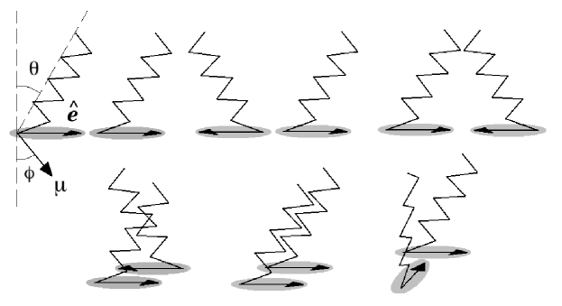
Figure 1: Schematic of representative effective-particle configurations and corresponding lipid chain orientations. Details given in the text.

Fig. 1 shows the most representative effective-particle configurations. Let us associate a two-dimensional unit vector $\hat{\bm{e}}_{i}$ with the $i$th molecule. This vector is on the plane of the monolayer and points along the projection of the lipid tail. Therefore, it is parallel to the long axis of the effective two-dimensional particle. If $\hat{\bm{r}}$ is the unit vector joining particle 1 with 2, we define $a_{i}=\hat{\bm{r}}\cdot\hat{\bm{e}}_{i}$ and $b=\hat{\bm{e}}_{1}\cdot\hat{\bm{e}}_{2}$. Then the three end-to-end configurations have $(b,a_{1},a_{2})=(+1,+1,+1)$, $(-1,\pm 1,\mp 1)$, while for the two side-to-side configurations $(b,a_{1},a_{2})=(+1,0,0)$ and $(-1,0,0)$. With the chain molecular structure in mind, it is clear that, as far as van der Waals interactions are concerned, the first two end-to-end configurations, $\rightarrow\rightarrow$ and $\rightarrow\leftarrow$, cannot have the same energy (note that the configurations $\rightarrow\leftarrow$ and $\leftarrow\rightarrow$ are taken as equivalent). Also, the two side-to-side configurations, $\uparrow\uparrow$ and $\uparrow\downarrow$, cannot have the same energy either. These two configurations contain the most important relative difference energetically: in the case $b=+1$ lipid chains are in complete contact, whereas in the second $b=-1$ they interact much less.

Thus, to the HR potential, an anisotropic attractive contribution between the effective particles is added. This contribution is intended to represent the van der Waals attraction between the lipid chains, and should be sensitive to the sign of $b$. The model for the attractive interaction will be a modified Gay-Berne (GB) potential GB . The GB potential is an anisotropic Lennard-Jones-like potential which has been extensively studied in three-dimensional fluids to account for interactions between anisotropic, mesogenic particles. However, its use in two-dimensional systems is scarce, probably because it predicts a continuous, rather than first order, phase transition between isotropic and nematic fluids. Since the original GB model presents head-to-tail symmetry, it cannot discriminate between the two side-to-side (or end-to-end) configurations, and a modification is required to introduce a splitting between the configurations.

In the original GB model the potential energy for two particles with relative centre-of-mass vector ${\bm{r}}={\bm{r}}_{2}-{\bm{r}}_{1}$ and orientations $\hat{\bm{e}}_{1}$ and $\hat{\bm{e}}_{2}$ is

$$\Phi_{\rm GB}({\bm{r}},\hat{\bm{e}}_{1},\hat{\bm{e}}_{2})=4\epsilon\left({\bm{r}},\hat{\bm{e}}_{1},\hat{\bm{e}}_{2},\right)f\left({\bm{r}},\hat{\bm{e}}_{1},\hat{\bm{e}}_{2}\right)$$ (1)

with

$$\epsilon\left({\bm{r}},\hat{\bm{e}}_{1},\hat{\bm{e}}_{2},\right)=\epsilon_{\rm GB}\epsilon_{1}^{\nu}\left(\hat{\bm{e}}_{1},\hat{\bm{e}}_{2}\right)\epsilon_{2}^{\mu}\left(\hat{\bm{r}},\hat{\bm{e}}_{1},\hat{\bm{e}}_{2}\right)$$ (2)

and

$$f\left({\bm{r}},\hat{\bm{e}}_{1},\hat{\bm{e}}_{2}\right)=\left(\frac{\sigma_{0}}{r-\sigma\left(\hat{\bm{r}},\hat{\bm{e}}_{1},\hat{\bm{e}}_{2}\right)+\sigma_{0}}\right)^{12}-\left(\frac{\sigma_{0}}{r-\sigma\left(\hat{\bm{r}},\hat{\bm{e}}_{1},\hat{\bm{e}}_{2}\right)+\sigma_{0}}\right)^{6}.$$ (3)

$\sigma\left(\hat{\bm{r}},\hat{\bm{e}}_{1},\hat{\bm{e}}_{2}\right)$ is a contact distance that depends on the relative particle angle $\hat{\bm{r}}$ and the two particle orientations $\hat{\bm{e}}_{1},\hat{\bm{e}}_{2}$. $\epsilon_{\rm GB}$ is an energy scale, while $\mu=2$ and $\nu=1$ are exponents. $\sigma_{0}$ is made to coincide with the particle width. In the standard Gay-Berne model the contact distance is given by the Hard-Gaussian Overlap (HGO) model. The full expressions are:

$$\sigma\left(\hat{\bm{r}},\hat{\bm{e}}_{1},\hat{\bm{e}}_{2}\right)=\sigma_{\rm HGO}\left(\hat{\bm{r}},\hat{\bm{e}}_{1},\hat{\bm{e}}_{2}\right)=\sigma_{0}\left\{1-\frac{\chi}{2}\left[\frac{\left(a_{1}+a_{2}\right)^{2}}{1+\chi b}+\frac{\left(a_{1}-a_{2}\right)^{2}}{1-\chi b}\right]\right\}^{-1/2},$$

$$\epsilon_{1}\left(\hat{\bm{e}}_{1},\hat{\bm{e}}_{2}\right)=\left\{1-\chi^{2}b^{2}\right\}^{-1/2},$$

$$\epsilon_{2}\left(\hat{\bm{r}},\hat{\bm{e}}_{1},\hat{\bm{e}}_{2}\right)=1-\frac{\chi^{\prime}}{2}\left[\frac{\left(a_{1}+a_{2}\right)^{2}}{1+\chi^{\prime}b}+\frac{\left(a_{1}-a_{2}\right)^{2}}{1-\chi^{\prime}b}\right],$$ (4)

where $\sigma_{\rm HGO}\left(\hat{\bm{r}},\hat{\bm{e}}_{1},\hat{\bm{e}}_{2}\right)$ is the contact distance of the HGO model (which closely approximates that of hard ellipses).

In our modified model, we introduce two variations to the standard GB model, Eqns. (4). The first is forced by the fact that the HGO model for the hard core does not produce a first-order phase transition between the isotropic and nematic phases. As discussed, this is a necessary requirement for the model in our application to coexisting domains in the monolayer (note that the presence of an attractive contribution in the GB model does not modify this scenario). To correct this unwanted feature, we have modified the hard core and adopted a HR shape. This model is known to exhibit a first-order transition from the isotropic phase to the uniaxial nematic phase in a range of aspect ratios Yuri . In particular, for an aspect ratio $\kappa=3$, the phase transition is of first order, and gives rise to a density gap with a sufficiently wide coexistence region. The modification involves substituting the contact distance in (4) by that of the HR model, $\sigma\left(\hat{\bm{r}},\hat{\bm{e}}_{1},\hat{\bm{e}}_{2}\right)=\sigma_{\rm HR}\left(\hat{\bm{r}},\hat{\bm{e}}_{1},\hat{\bm{e}}_{2}\right)$.

Figure 2: Modified Gay-Berne potential for various relative configurations of two molecules. $\hat{\bm{e}}$ vectors for each configuration are indicated as arrows. Values of the parameters are $\kappa=3$, $\kappa^{\prime}=0.3$, $\mu=2$ and $\nu=1$. (a) $\delta=0$. (b) $\delta=1.5$.

The second modification involves splitting the energy of parallel $b=+1$ and antiparallel $b=-1$ configurations, as discussed above. The simplest way to implement this feature is by modifying the $\epsilon_{1}$ function to

$$\epsilon_{1}\left(\hat{\bm{e}}_{1},\hat{\bm{e}}_{2}\right)=\left\{1-\frac{1}{2}\chi^{2}(1+\delta b)\right\}^{-1/2},$$ (5)

where $\delta$ is an asymmetry parameter that quantifies the energy splitting. The resulting modified potential (1) with (5) instead of (4) for the energy function $\epsilon_{1}$ will be called Modified Gay-Berne (MGB) potential, $\Phi_{\rm MGB}({\bm{r}},\hat{\bm{e}}_{1},\hat{\bm{e}}_{2})$. Note that $\delta=0$ does not reduce (5) to the standard GB model.

Fig. 2 shows the MGB potential for various selected relative configurations of two particles: the two side-to-side configurations $\uparrow\uparrow$ and $\uparrow\downarrow$, the two T configurations $\uparrow\leftarrow$ and $\uparrow\rightarrow$, and the two side-to-side configurations $\rightarrow\rightarrow$ and $\rightarrow\leftarrow$. The parameter $\kappa^{\prime}$ describes the relative energy between parallel and T configurations in the original GB potential, and is set to $0.3$. In the figure results for two different values of the $\delta$ are shown: $\delta=0$, panel (a), and $\delta=1.5$, panel (b). We see how the two side-to-side configurations are degenerate for $\delta=0$ but split into two distinct levels for $\delta>0$. The end-to-end configurations are also affected by $\delta$, but not the T configurations, which remain degenerate.

Therefore our model represents lipid molecules as two-dimensional elongated objects (on the plane of the monolayer), interacting through anisotropic van der Waals forces. Note that, in our model, interactions between the effective particles do not depend on the phase these particles belong to. This means that interactions are not sensitive to the chain disorder of molecules in the LE phase, as opposed to the perfect chain order in the LC phase. This shortcoming of the model could be overcome by considering an additional particle variable accounting for the mean number of defects along the lipid chains. The variable would be coupled to the other variables through modification of the energy prefactors in (4). However, we believe that the impact of assuming that interactions do not depend on chain ordering is negligible in view of the fact that our results for the line tension are in reasonable agreement with experiment, as commented below.

In addition to the van der Waals interaction, an embedded linear dipole pointing along some direction (not necessarily oriented in the plane) in included. This dipole represents the joint electrostatic charges of the neutral head group of the lipid molecule. The pair potential energy is written as a sum of two contributions, the modified Gay-Berne term and the dipole energy:

$$\Phi({\bm{r}}_{12},\hat{\bm{e}}_{1},\hat{\bm{e}}_{2})=\Phi_{\rm MGB}({\bm{r}},\hat{\bm{e}}_{1},\hat{\bm{e}}_{2})+\Phi_{\rm dip}({\bm{r}},\hat{\bm{e}}_{1},\hat{\bm{e}}_{2}).$$ (6)

The dipolar energy term is

$$\Phi_{\rm dip}(\hat{\bm{r}},\hat{\bm{e}}_{1},\hat{\bm{e}}_{2}) = \frac{\mu_{\perp}^{2}}{\epsilon_{0}\epsilon_{\parallel}r^{3}}+\frac{\mu_{\parallel}^{2}}{\epsilon_{0}\epsilon_{\perp}r^{3}}\left[\hat{\bm{e}}_{1}\cdot\hat{\bm{e}}_{2}-3\left(\hat{\bm{e}}_{1}\cdot\hat{\bm{r}}\right)\left(\hat{\bm{e}}_{2}\cdot\hat{\bm{r}}\right)\right]=\frac{\mu_{\perp}^{2}}{\epsilon_{0}\epsilon_{\parallel}r^{3}}+\frac{\mu_{\parallel}^{2}}{\epsilon_{0}\epsilon_{\perp}r^{3}}\left(b-3a_{1}a_{2}\right).$$ (7)

The dipole may have components normal and parallel to the monolayer, respectively $\mu_{\perp}=\mu\cos{\theta}$ and $\mu_{\parallel}=\mu\sin{\theta}$, where $\theta$ is the polar angle of the dipole moment. In this dipolar model we are assuming that the dielectric constants in the two directions may be different. Atomistic simulations indicate that the angle $\theta$ in both LC and LE domains is very close to $22^{\circ}$. As regards the parallel component, it is assumed to be aligned along the long axis of the effective projected particle, $\hat{\bm{e}}$. This assumption is at variance with the results of the latter simulation, which predicts a parallel component that librates in the azimuthal angle, essentially uncorrelated with $\hat{\bm{e}}$. This result may be a feature of the force field used in the simulations and should be confirmed. In our model this situation would correspond to setting the in-plane component of the dipole $\mu_{\parallel}$ to zero. Note that the model does not contemplate the situation where $\hat{\bm{e}}$ is not in the plane spanned by the dipole moment and the normal to the monolayer.

With this model we attempt to describe a phase diagram involving two phases, one with orientational disorder (equivalent to the LE phase of the lipid monolayer) and another with orientational order (akin to the LC phase). Also, the effect of the dipolar strength on the coexistence gap can be studied, along with the stability and shape of domains, and eventually some dynamical aspects of domain growth. Some of these issues are addressed in the present study. Others will be left for future work.

As formulated, the model is expected to present a number of stable equilibrium phases. Among these are the isotropic phase, where molecules are both spatially and orientationally disordered, and the nematic phase, a fluid phase where molecules are oriented on average along some common direction, called the director. The model also contains an exotic nematic phase, the tetratic, which is a fluid phase with two equivalent directors. The tetratic can replace the standard nematic phase when the aspect ratio of the particles is sufficiently low. Also the model exhibits a crystalline, fully ordered phase at high density. The existence of this sequence of stable phases is based on the known properties of the hard core interaction of the model, the HR model, which are well known. These and related models have been studied theoretically using mean-field theory Yuri ; B3 and by means of simulation Stillinger . In contrast, the effect of the addition of an anisotropic attractive interaction and a linear dipole has not been investigated. Although the nature of the stable phases is not expected to be modified (based on similar models in two and three dimensions), the effect of the new ingredients will certainly be a profound one. In particular, we would like to obtain some trends as to the effect of the dipole orientation and strength. Initially we formulate a general model and explore the consequences on phase behaviour.

The model is here analysed using classical density-functional theory (DFT) and associated mean-field approximations to examine the phase behaviour. At this point we neglect non-uniform spatial ordering since the introduction of this order in the theory gives rise to an unnecessarily complicated numerical problem. Therefore, at the DFT level we restrict ourselves to a description of the uniform phases, i.e. isotropic and nematic (we choose the aspect ratio of the particles in such a way as to avoid the stabilisation of tetratic ordering, which is certainly not observed in lipid monolayers). These phases will be identified respectively with the LE and LC phases.

One crucial assumption of our approach concerns the identification of the phases. The isotropic phase of the model is identified with the Liquid Expanded (LE) phase of the monolayer, while the nematic phase is meant to represent the Liquid Condensed (LC) phase. This may not be a realistic representation, especially in the case of the LC phase, but at least the model has two essential ingredients: in the LC phase the aliphatic chains of the molecules are rigid and oriented to optimise the van der Waals energy; and the components of the dipolar moment on the monolayer should be aligned and contribute to a global dipolar moment.

We now formulate a perturbation theory, taking the HR model as reference system. We write the one-particle density, Without loss of generality, as $\rho({\bm{r}},\hat{\bm{e}})=\rho({\bm{r}})f({\bm{r}},\hat{\bm{e}})$, where $\rho({\bm{r}})$ is the local number density and $f({\bm{r}},\hat{\bm{e}})$ the orientational distribution function. In the isotropic phase $f({\bm{r}},\hat{\bm{e}})=\frac{1}{2\pi}$, since the distribution function has to be normalised:

$$\int d\hat{\bm{e}}f({\bm{r}},\hat{\bm{e}})=\int_{0}^{2\varphi}d\varphi f({\bm{r}},\varphi)=1.$$ (8)

Now the potential energy is split into hard repulsive and attractive parts using a Barker-Henderson scheme. Then we write a free-energy functional as a sum of ideal and excess part, with the latter containing contributions from the MGB and dipolar terms:

$$F[\rho]=F_{\rm id}[\rho]+F_{\rm HR}[\rho]+F_{\rm MGB}[\rho]+F_{\rm dip}[\rho]$$ (9)

where

$$\beta F_{\rm id}[\rho] = \int d{\bm{r}}\int d\hat{\bm{e}}\rho({\bm{r}},\hat{\bm{e}})\left\{\log{\left[\rho({\bm{r}},\hat{\bm{e}})\Lambda^{2}\right]}-1\right\}$$ (10)

$$= \int d{\bm{r}}\rho({\bm{r}})\left\{\log{\left[\frac{\rho({\bm{r}})}{2\pi}\Lambda^{2}\right]}-1+\int d\hat{\bm{e}}f({\bm{r}},\hat{\bm{e}})\log{\left[2\pi f({\bm{r}},\hat{\bm{e}})\right]}\right\},$$

is the ideal free-energy contribution. $\Lambda$ is the thermal wavelength. The hard-core contribution can be written as

$$\beta F_{\rm HR}[\rho] = \psi_{\rm HR}(\rho_{0})\int d{\bm{r}}_{1}\int d\hat{\bm{e}}_{1}\rho({\bm{r}}_{1},\hat{\bm{e}}_{1})\int d{\bm{r}}_{2}\int d\hat{\bm{e}}_{2}\rho({\bm{r}}_{2},\hat{\bm{e}}_{2})v_{\rm exc}({\bm{r}}_{2}-{\bm{r}}_{1},\hat{\bm{e}}_{1},\hat{\bm{e}}_{2}),$$ (11)

where

$$v_{\rm exc}({\bm{r}},\hat{\bm{e}}_{1},\hat{\bm{e}}_{2})=\left\{\begin{array}[]{ll}\displaystyle 1,&r<\sigma_{\rm HC}(\hat{\bm{r}},\hat{\bm{e}}_{1},\hat{\bm{e}}_{2})\\ 0,&r>\sigma_{\rm HC}(\hat{\bm{r}},\hat{\bm{e}}_{1},\hat{\bm{e}}_{2})\end{array}\right\}=\Theta\left[\sigma_{\rm HC}(\hat{\bm{r}},\hat{\bm{e}}_{1},\hat{\bm{e}}_{2})-r\right]$$ (14)

is the overlap function, and $\rho_{0}$ is the mean density. The exact formulation of this functional depends on the hard-core model considered. In the case of HR, scaled-particle theory has been implemented in the past Yuri , and this is the theory used here. Also,

$$F_{\rm MGB}[\rho] = \frac{1}{2}\int d{\bm{r}}_{1}\int d\hat{\bm{e}}_{1}\rho({\bm{r}}_{1},\hat{\bm{e}}_{1})\int d{\bm{r}}_{2}\int d\hat{\bm{e}}_{2}\rho({\bm{r}}_{2},\hat{\bm{e}}_{2})$$ (15)

$$\hskip 56.9055pt\times\Theta\left[\left|{\bm{r}}_{2}-{\bm{r}}_{1}\right|-\sigma_{\rm HC}\left(\hat{\bm{r}}_{12},\hat{\bm{e}}_{1},\hat{\bm{e}}_{2}\right)\right]\Phi_{\rm MGB}({\bm{r}}_{2}-{\bm{r}}_{1},\hat{\bm{e}}_{1},\hat{\bm{e}}_{2})$$

is the attractive MGB contribution to the free energy. Finally

$$F_{\rm dip}[\rho] = \frac{1}{2}\int d{\bm{r}}_{1}\int d\hat{\bm{e}}_{1}\rho({\bm{r}}_{1},\hat{\bm{e}}_{1})\int d{\bm{r}}_{2}\int d\hat{\bm{e}}_{2}\rho({\bm{r}}_{2},\hat{\bm{e}}_{2})$$ (16)

$$\hskip 56.9055pt\times\Theta\left[\left|{\bm{r}}_{2}-{\bm{r}}_{1}\right|-\sigma_{\rm HR}\left(\hat{\bm{r}}_{12},\hat{\bm{e}}_{1},\hat{\bm{e}}_{2}\right)\right]\Phi_{\rm dip}({\bm{r}}_{2}-{\bm{r}}_{1},\hat{\bm{e}}_{1},\hat{\bm{e}}_{2})$$

is the dipolar contribution. In these expression we are assuming that correlations are given by a simple step function (i.e. only the correlation hole is taken into account).

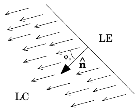
Figure 3: Definition of the angle $\varphi_{0}$ at the boundary between LE and LC domains. Arrows represent the orientation of the local director, which is taken to be uniform in our model. $\hat{\bm{n}}$ is the unit vector along the inward normal.

Now we give some details on how the theory is solved. We only sketch the basic approximations and the numerical approach, considering the more general interfacial case; the thermodynamics of the bulk phases can be obtained from the same interfacial approach, using the corresponding bulk distributions. The interfacial structure is computed using a variational method, where the density $\rho(x)$ and a set of orientational parameters $\{\Lambda_{n}(x)\}$ are taken as variational functions. In the context of the present mean-field approach, we do not consider fluctuations of the boundary and instead assume a flat boundary. The reference axis $x$ is taken along the boundary normal. This means that the variational parameters, $\rho(x)$ and $\{\Lambda_{n}(x)\}$, will be functions of the $x$ coordinate only. The orientational distribution function is then $f(x,\varphi)=f(\varphi;\{\Lambda_{n}(x)\})$, where $\varphi$ is the angle between the long axis of a particle $\hat{\bm{e}}$ and the $x$ axis of the lab reference frame. The following parameterisation is used:

$$f(x,\varphi)=\frac{\displaystyle e^{\displaystyle\sum_{n=1}^{\infty}\Lambda_{n}(x)\cos{n\left(\varphi-\varphi_{0}\right)}}}{\displaystyle\int_{0}^{2\pi}d\varphi^{\prime}e^{\displaystyle\sum_{n=1}^{\infty}\Lambda_{n}(x)\cos{n\varphi^{\prime}}}}.$$ (17)

In this expression we allow for the possibility that, in the nematic phase, the director is oriented at an angle different from the normal direction. This effect is central to our discussion and is taken into account through the angle $\varphi_{0}$ in (17), which implies a global rotation of the director, see Fig. 3. The parameters $\{\Lambda_{n}(x)\}$ at each position $x$ will be a measure of particle ordering about the direction dictated by $\varphi_{0}$. Note that in this work we do not assume a spatial dependence of the angle $\varphi_{0}$, which means that the director is uniform across the boundary with no deformation. This assumption is based on our choice of a flat geometry for the boundary and on our inability to tackle the more general problem of boundary deformations and fluctuations within the present formulation. We limit the number of variational parameters to the first two parameters, $\Lambda_{1}(x)$ and $\Lambda_{2}(x)$, which contain the symmetry of the polar and uniaxial nematic phases. Once the equilibrium values of $\Lambda_{1}(x)$ and $\Lambda_{2}(x)$ are obtained, the corresponding local order parameters $s_{1}(x)$ and $s_{2}(x)$ in the proper frame (i.e. the frame associated with the nematic director) can be obtained from

$$s_{n}(x)=\int_{0}^{2\pi}d\varphi f(x;{\varphi})\cos{n(\varphi-\varphi_{0})}.$$ (18)

The minimisation is realised by discretising the spatial coordinates, which turns the problem into a minimisation problem of a function of many variables, i.e. all the values of $\rho$, $\Lambda_{1}$ and $\Lambda_{2}$ at the discrete points defined along the $x$ axis. Due to the long-range nature of the dipolar interactions, many such points have be defined, meaning that the computation box containing the interfacial boundary between the isotropic and nematic phases will be very long in the direction normal to the boundary. The cutoff in the interactions is set to $30\sigma_{0}$. We have used a box of length $100\sigma_{0}$ in the direction normal to the interface, with a grid size $\Delta x=0.1\sigma_{0}$ (the effective box length is in fact extended to $160\sigma_{0}$ to take into account the nonlocal interactions).

Using the property of translational invariance in the direction of the flat boundary ($y$ axis), all integrals over ${\bm{r}}_{1}=(x_{1},y_{1})$ and ${\bm{r}}_{2}=(x_{2},y_{2})$ in Eqns. (11), (15) and (16) can be written as integrals along $x$ coordinates only. In the process, effective potentials $\tilde{v}_{\rm exc}(x,\varphi_{1},\varphi_{2})$, $\tilde{\Phi}_{\rm MGB}(x,\varphi_{1},\varphi_{2})$ and $\tilde{\Phi}_{\rm dip}(x,\varphi_{1},\varphi_{2})$, are defined, which can be computed in advance. These effective potentials are already integrated in the $y$ coordinates, and incorporate the correlation hole given by the Heaviside function. For example, in the case of the dipolar term, we have:

$$F_{\rm dip}[\rho] = \frac{L}{2}\int_{-\infty}^{\infty}dx_{1}\rho(x_{1})\int_{-\infty}^{\infty}dx_{2}\rho(x_{2})$$ (19)

$$\times \int_{0}^{2\pi}d\varphi_{1}\int_{0}^{2\pi}d\varphi_{2}f\left(\varphi_{1};\Lambda_{1}(x_{1}),\Lambda_{2}(x_{1})\right)f\left(\varphi_{2};\Lambda_{1}(x_{2}),\Lambda_{2}(x_{2})\right)\tilde{\Phi}_{\rm dip}(x_{1}-x_{2},\varphi_{1},\varphi_{2}).$$

The factor $L$, which represents the length of the (flat) boundary, comes by invoking translational invariance along the boundary, which is expressed by the presence of the factor $y_{1}-y_{2}$. The calculation of integrals such as those in (19), which have the same structure in the case of the other free-energy contributions, involves a serious numerical burden. We must bear in mind that a minimisation process over many variables is imposed on the full free-energy functional, and this process involves a very large number of free-energy evaluations.

Our strategy was to evaluate the double angular integrals in a single step before the minimisations. For example, for the dipolar term, we evaluate

$$V_{\rm dip}(\Lambda_{1}^{(1)},\Lambda_{2}^{(1)},\Lambda_{1}^{(2)},\Lambda_{2}^{(2)})$$

$$\hskip 28.45274pt\equiv\int_{0}^{2\pi}d\varphi_{1}\int_{0}^{2\pi}d\varphi_{2}f\left(\varphi_{1};\Lambda_{1}(x_{1}),\Lambda_{2}(x_{1})\right)f\left(\varphi_{2};\Lambda_{1}(x_{2}),\Lambda_{2}(x_{2})\right)\tilde{\Phi}_{\rm dip}(x_{1}-x_{2},\varphi_{1},\varphi_{2}),$$ (20)

and create a large table with four entries: the values of two parameters $\Lambda_{1},\Lambda_{2}$ evaluated at the first particle (coordinates with subindex $1$) and the values of two parameters $\Lambda_{1},\Lambda_{2}$ evaluated at the second particle (coordinates with subindex $2$), i.e. $\Lambda_{1}^{(1)}\equiv\Lambda_{1}(x_{1})$, $\Lambda_{2}^{(1)}\equiv\Lambda_{2}(x_{1})$, $\Lambda_{1}^{(2)}\equiv\Lambda_{1}(x_{2})$ and $\Lambda_{2}^{(2)}\equiv\Lambda_{2}(x_{2})$. This table is then interpolated for intermediate values of the parameters. The accuracy of this procedure is reasonable. The same procedure is applied to the other free-energy contributions. This strategy saves a lot of computer time and simplifies the boundary calculations considerably.

The relevant free-energy function to minimise is the line tension, which is defined as the excess grand potential per unit length, $\lambda=(\Omega-\Omega_{0})/L$, where $\Omega=F-\mu N$ is the grand potential, $L$ the interface length, $\mu$ the chemical potential at coexistence, $N$ the number of particles, and $\Omega_{0}$ is the bulk grand potential. The line tension is minimised with respect to all the independent variables defined on the discretised $x$ axis, $\rho(x)$, $\Lambda_{1}(x)$ and $\Lambda_{2}(x)$, using a conjugate-gradient method. In each case the angle $\varphi_{0}$ between the nematic director and the monolayer normal is fixed at some value in the interval $[0^{\circ},180^{\circ}]$. This process recovers the bulk results and bulk coexistence very accurately. However, despite the numerical accuracy of our strategy, very small deviations exist for the bulk properties at different values of $\varphi_{0}$. This is a problem since the computation box is assumed to be coupled to bulk isotropic and nematic phases at each side of the box, and definite coexistence values for density and order parameters, consistent with the numericals of the interfacial problem, have to be fixed as boundary conditions. Any minor difference in the boundary conditions will be detrimental for the correct minimisation. The solution is to obtain the bulk coexistence consistently for each value of $\varphi_{0}$, which ensures perfect matching and a smooth minimisation process.

For the bulk phases we assume the dependence $\rho(x)=\rho_{0}$ and $f(x;\varphi)=f(\varphi)$ for the phase with the lowest symmetry, the nematic phase. In the isotropic phase $f(\varphi)=1/2\pi$. In this case we numerically minimise the total Helmholtz free-energy functional, using the same strategy as for the interface. Once the equilibrium (constant) values of the $\Lambda_{1}$ and $\Lambda_{2}$ parameters are obtained for the nematic phase, the order parameters and the equilibrium free energy can be evaluated. From this the chemical potential and the pressure can be computed numerically, and the whole phase diagram obtained by applying the equal-pressure and equal-chemical potential conditions at each temperature $T$.

Results and discussion

For both bulk and interface three cases have been analysed: zero dipole, dipole in the plane of the monolayer, and dipole perpendicular to the monolayer. The asymmetry parameter $\delta$ is fixed to a value $\delta=1.5$. This value gives an energy gap between parallel and antiparallel configurations of $58\%$ (see Fig. 2). As discussed previously, we do not claim this value to be representative of any realistic situation. We simply argue that $\delta$ reflects the asymmetry between the two unequivalent configurations of two tilted molecular chains, and that larger tilt angles may reasonably be associated with larger values of $\delta$. A proper connection between the atomistic model and the effective two-dimensional model can be done, but is outside the scope of this exploratory investigation. Larger values of $\delta$, giving stronger energy anisotropies, on the other hand, do not substantially change the results and the qualitative conclusions that can be drawn from the model. In order to check this point, a value $\delta=1.75$, giving an energy gap of $69\%$, was also explored. There is a technical problem with the value of the asymmetry parameter, since in the model the value of $\delta$ cannot be chosen arbitrarily. For example, for clearly smaller values the density gap of the isotropic-nematic transition becomes extremely small or even disappears, which is not realistic for the present application. In practice we have checked that $1.5$ is slightly above the limiting value below which a realistic density gap for the isotropic-nematic transition cannot be obtained. What we mean by ‘realistic density gap’ will be discussed below.

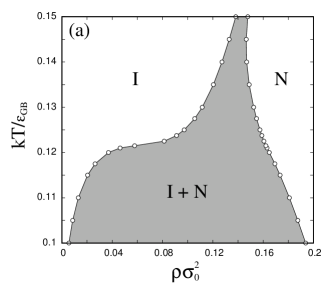
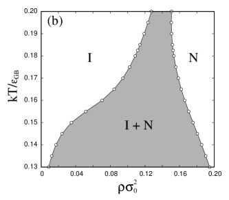
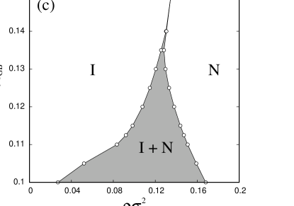
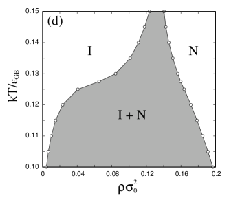
Figure 4: Phase diagrams for different values of the parameters. (a) $\delta=1.5$, $\mu^{*}_{\perp}=0$, $\mu^{*}_{\parallel}=0$. (b) $\delta=1.75$, $\mu^{*}_{\perp}=0$, $\mu^{*}_{\parallel}=0$. (c) $\delta=1.5$, $\mu^{*}_{\perp}=0.6$, $\mu^{*}_{\parallel}=0$. And (d) $\delta=1.5$, $\mu^{*}_{\perp}=0$, $\mu^{*}_{\parallel}=0.6$.

Fig. 4 presents four phase diagrams in the temperature-density plane corresponding to the cases mentioned above. All quantities are scaled with the appropriate parameters to give dimensionless quantities, $\epsilon_{\rm GB}$ for energies and $\sigma_{0}$ for lengths. In the case of the dipolar strengths we scale as $\mu_{i}^{*}=\mu_{i}/\sqrt{\epsilon_{0}\epsilon_{i}\epsilon_{\rm GB}\sigma_{0}^{3}}$, with $i=\parallel,\perp$. All phase diagrams present a common feature: the existence of a transition between an isotropic (LE) phase and a nematic (LC) phase. In all cases the transition is of first order and preempts the isotropic-vapour transition, which is metastable and below the two isotropic-nematic binodal curves. The latter feature is not a limitation of the model for the present study, which focusses on the phase coexistence between orientationally ordered and disordered phases. Also in all cases the density gap between isotropic and nematic phases rapidly decreases with temperature and eventually closes, giving rise to a continuous phase transition at a tricritical point. In real monolayers the density gap disappears at a critical point, above which LC and LE regions can be continuously connected. The different symmetries of the phases involved in our model and the absence of fluctuations in our mean-field treatment precludes the existence of a critical point. Again this shortcoming is not an essential point for our purposes. Note that, for even higher temperatures, the density gap has to return to a finite value since the infinite-temperature limit of the model is the HR model, which exhibits a first-order transition Yuri .

We first compare panels (a) and (b) of Fig. 4, both corresponding to zero dipole but for different values of $\delta$. It is clear that an increasing anisotropy, producing a larger energy gap, does not shift the isotropic-nematic transition in temperature, but gives rise to an increased density gap. Similar conclusion are drawn from a comparison of panels (a) and (d), corresponding to the same value of $\delta$ but to zero dipole and purely inplane dipole, respectively. There exists an incipient isotropic-vapour transition, and the inplane dipole slightly weakens the anisotropic interactions of the MGB model and promotes the stability of the nematic phase. But more importantly, the inplane dipole does not qualitatively affect the phase diagram.

By contrast, the case of a purely perpendicular dipole component, panel (c), is qualitatively different. Condensation of the isotropic phase is clearly discouraged, since the perpendicular dipole introduces a purely repulsive interaction. Also, the effective anisotropic interactions promoting the ordering transition decrease, with the result that the density gap at a given temperature is considerably reduced, and the tricritical point (not visible in the scale of the other panels) moves to lower temperatures.

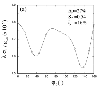
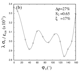
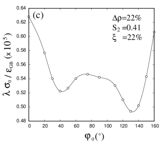
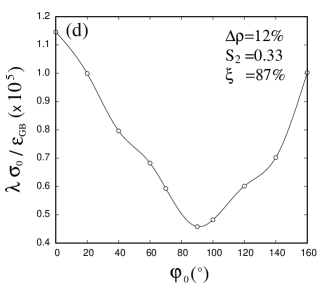
Figure 5: Line tension as a function of the molecular orientation with respect to the domain boundary normal. (a) $\delta=1.5$, $\mu^{*}_{\parallel}=0$, $\mu^{*}_{\perp}=0$ ($kT/\epsilon_{\rm GB}=0.13$), (b) $\delta=1.75$, $\mu^{*}_{\parallel}=0$, $\mu^{*}_{\perp}=0$ ($kT/\epsilon_{\rm GB}=0.1825$). (c) $\delta=1.5$, $\mu^{*}_{\parallel}=0$, $\mu^{*}_{\perp}=0.6$ ($kT/\epsilon_{\rm GB}=0.12$). (d) $\delta=1.5$, $\mu^{*}_{\parallel}=0.6$, $\mu^{*}_{\perp}=0$ ($kT/\epsilon_{\rm GB}=0.15$). Continuous line is a cubic spline fitting intended only as a guide to the eye.

Fig. 5 presents the line tension $\lambda(\varphi_{0})$ as a function of the angle $\varphi_{0}$ between the average projection of the molecular chains in the LC domains (director) and the normal to the phase boundary $\hat{\bm{n}}$, see Fig. 3. The four panels correspond to the four cases shown in Fig. 4. As a reference, in each case the value of the temperature is chosen such that the density gap is close or of the same order as that observed in the atomistic simulations us , which is approximately $27\%$ with respect to the density of the LC phase. Therefore the temperatures are $kT/\epsilon_{\rm GB}=0.13$ in panel (a), $0.1825$ in panel (b), $0.12$ in panel (c) and $0.15$ in panel (d), giving density gaps of $27\%$, $27\%$, $22\%$ and $12\%$, respectively.

The first observation is that the line tension is considerably reduced when dipole interactions, either perpendicular or parallel to the monolayer, are introduced. This reduction cannot be explained alone by the density gap since their values are similar, see e.g. panels (a) and (c). Also, the gap in the order parameters, e.g. the nematic order parameter $S_{2}$, at the transition, cannot explain by itself the drop in line tension. The conclusion is that the dipolar interactions are responsible for the substantial reduction in $\lambda$. Experimental values of $\lambda$ for lipid monolayers, extracted from domain size distributions Israelachvili , are in the range $1-10$ fN (although values measured using other techniques may be higher by even two orders of magnitude depending on the system CWT ; line_tension1 ; line_tension2 ). Using $\sigma_{0}\sim 0.4$ nm (estimated from experimental values of area per lipid in LC domains of DPPC monolayers) and $\epsilon_{\rm GB}\sim 50$ kT (estimated from atomistic force-field simulations us , and see also Libro_Israel ), we obtain values of $\lambda\sim 2-15$ fN, i. e. within the same order of magnitude as in Israelachvili .

Interestingly, line tensions exhibit well-defined minima which correspond to equilibrium oblique configurations at the boundary between LE and LC phases. This is indicating the existence of an anisotropic line tension. In cases where no dipole exists, panels (a) and (b), there is a global minimum at $\varphi_{0}\simeq 135^{\circ}$ and a local minimum at $\varphi_{0}\simeq 40^{\circ}$. These two angles are close to being supplementary angles, which means that, in both configurations, the long axes of the effective particles lie on the same straight line, but the projected chains point in opposite directions. The most stable configuration corresponds to chains pointing towards the bulk of LE regions at an angle of $135^{\circ}-90^{\circ}=45^{\circ}$ with respect to the boundary. Panel (c) corresponds to a model where a dipole perpendicular to the monolayer is added. Clearly, the barrier between minima is reduced, but the location of the minima does not change. This indicates that a perpendicular dipole does not affect the anisotropy introduced by the MGB component. Finally, in panel (d) a purely inplane dipole has been added. In this case the situation drastically changes, as only one minimum is visible at a angle of $\varphi_{0}=90^{\circ}$. This corresponds to molecular projections parallel to the phase boundary. In all cases the line tension is anisotropic, meaning that the interface pins the molecular orientation, which is transmitted to the bulk via elastic forces, a situation similar to the anchoring phenomena in liquid crystals.

Another interesting question is the degree of anisotropy of the line tension. A possible measure of the anisotropy, $\xi$, is given by the amplitude of its variation in the whole range of $\varphi_{0}$, $\Delta\lambda$, divided by the mean value $\lambda_{0}$, i.e. $\xi=\Delta\lambda/\lambda_{0}$. In the cases shown in Fig. 5 the values for the anisotropy are $\xi=0.16$, $0.22$ and $0.87$ in panels (a), (c) and (d), respectively. Dipolar interactions parallel to the monolayer have a profound impact on the line-tension anisotropy, whereas the perpendicular components also add some anisotropy over that of the pure MGB potential which, at $\xi=16\%$, is already substantial. We are not aware of any experimental values for the anisotropy.

These results should be compared with available evidence on molecular structure and ordering. An important source of information comes from atomistic computer simulations. Two such simulations on DPPC monolayers have recently been published Javanainen ; us . The two use the same force fields and the only difference is system size. We focus on Ref. Javanainen , in which complete phase separation was probed along the coexistence region, and pictures of representative molecular configurations were shown. Invariably, an angle $\varphi_{0}$ at the domain boundaries different from $90^{\circ}$ can be seen in the configurations. Direct visual estimates of the angle provide a value of $\sim 27^{\circ}$ (see panel 3, Fig. 2 of Ref. Javanainen ).

The above results imply that the inplane dipolar component cannot be large, or at least cannot influence the structural properties of the domain. This is supported by the results of Ref. us that the inplane component of the dipoles show almost complete librational motion about the monolayer normal. This could imply that the inplane dipolar components of neighbouring molecules interact weakly, because of strong screening Moy or otherwise. Therefore, the only relevant or effective dipolar component would be the perpendicular one. The line tension is strongly affected by this component, which reduces its value. The angular anisotropy of the line tension, which is otherwise contained in the model with no dipole interactions, increases moderately when perpendicular dipole forces are present. However, the main contribution of the anisotropy is due to the molecular tilt, and the perpendicular dipoles only contribute to a lesser extent. The angular dependence of the line tension can be represented by

$$\lambda(\varphi_{0})=\lambda_{0}+\sum_{n=1}^{\infty}\lambda_{n}\cos{n\varphi_{0}}.$$ (21)

The different behaviours shown in Fig. 5 can be explained in terms of the $n=1,2,3$ and $4$ components. Minima at $\simeq 45^{\circ}$ and $135^{\circ}$ are due to the $n=4$ term. The $n=1$ and $3$ components affect the relative stability of these two minima. The minimum at $90^{\circ}$ is due to the $n=2$ component. A model potential with no gap between $\uparrow\uparrow$ and $\uparrow\downarrow$ configurations promotes a $90^{\circ}$ angle at the boundary Yuri1 (planar orientation). Inplane dipoles also favour this configuration. The presence of a tilt-induced gap is responsible for the preferred orientations at oblique angles.

Competition between bulk interactions from perpendicular dipoles and an isotropic line tension $\lambda_{0}$ has been invoked as a mechanism to determine domain shape in mesoscopic models. Dipole interactions promote elongated shapes, which are counterbalanced by an isotropic line tension. Different shape regimes emerge from this competition. However, the angle-dependent terms (21), which are present even in the absence of dipolar interactions, play the same role as these interactions. In this alternative scenario, long linear sectors of the domain boundary would optimise the line free energy, thus favouring the formation of elongated domains with long linear boundaries. In fact, the results presented in this section correspond to a value of the line-tension-to-dipolar strength ratio of $\Lambda=\lambda_{0}^{*}/(\mu_{\perp}^{*}\Delta\rho^{*})^{2}\simeq 0.02$, i.e. to a regime dominated by dipolar interactions. A reduction of $\mu_{\perp}^{*}$ to $0.1$ would increase $\Lambda$ to $\sim 1$. Even in this case domains with a high number of lobes are stabilised, according to mesoscopic models domains1 ; Aurora . Anisotropic line tensions are expected to suppress or at least reduce the stability of these highly-lobed structures in favour of shapes with lower overall curvature.

Summary and conclusions

In this work we have formulated a very simple model to study the interfacial structure at the boundary between LC and LE domains in DPPC monolayers. The model predicts an anisotropic line tension $\lambda(\varphi_{0})$ with respect to the angle $\varphi_{0}$ between the nematic director (which describes orientation of the projected molecular chains in LC domains) and the normal to the boundary. The minimum line tension occurs at oblique angles, which is in agreement with results from atomistic simulation us ; Javanainen . Anisotropy in the line tension is already implicit in a model with only van der Waals lipid chain interactions (modified Gay-Berne potential), and dipolar components perpendicular to the monolayer only marginally increase the anisotropy. Indirectly our model also supports the concept that inplane dipolar components should have a minor role in the value of line tension since these components favour a planar orientation at the boundary, which is incompatible with the results from atomistic simulations. This may be explained by the stronger screening of inplane dipoles as compared to perpendicular dipoles.

Our results indicate that theoretical mesoscopic models aimed at predicting domain shape and domain shape transitions should be extended to account for anisotropy in the line tension. On the one hand, inplane dipolar components may not be relevant to construct realistic models (see Ref. Moy where the effect of such contributions is discussed). On the other, models with perpendicular dipoles should also reflect the anisotropy in the line tension stemming from the combined effect of nonzero tilt angles of lipid chains and perpendicular dipoles. We should recall that all atomistic simulations to date consistently predict nonzero lipid-chain tilt angles in LC domains. In our model, the perpendicular dipole component seems to play an important role in reducing the line tension, but only induces a small incremental anisotropy. Of course, competition between (long-range) dipolar bulk interactions and line tension is a relevant factor for the global domain morphology, as indicated by mesoscopic models domains1 ; domains2 ; Aurora , but an anisotropic line tension may be a crucial requirement.

References

- (1) Pérez-Gil, J.; Wüstneck, N.; Cruz, A.; Fainerman, V. B.; Pison, U. Interfacial properties of pulmonary surfactant layers, Adv. Coll. Interf. Sci. 2005, 117, 33-58.
- (2) Casals, C.; Cañadas, O. Role of Lipid Ordered/Disordered Phase Coexistence in Pulmonay Surfactant Function, Biochim. et Biophys. Acta 2012, 1818, 2550-2562.
- (3) Kaganer, V. M.; Möhwald, H.; Dutta, P. Structure and Phase Transitions in Langmuir Monolayers, Rev. Mod. Phys. 1999, 71, 778-891.
- (4) Moy, V. T.; Keller, D. J.; Gaub, H. E.; McConnell, H. M. Long-Range Molecular Orientational Order in Monolayer Solid Domains of Phospholipid, J. Phys. Chem. 1986, 90, 3198-3202.
- (5) Keller, D. J.; Korb, J. P.; McConnell, H. M. Theory of Shape Transitions in Two-Dimensional Phospholipid Domains, J. Phys. Chem. 1987, 91, 6417-6422.
- (6) Campelo, F.; Cruz, A.; Pérez-Gil, J.; Vázquez, L.; Hernández-Machado, A. Phase-field Model for the Morphology of Monolayer Lipid Domains, Eur. Phys. J. E 2012, 35, 49.
- (7) Ipsen, J. H.; Mouritsen, O. G.; Zuckermann, M. J. Decoupling of crystalline and conformational degrees of freedom in lipid monolayers, J. Chem. Phys. 1989, 91, 1855-1865.
- (8) Mouritsen, O. G.; Zuckermann, M. J. Acyl chain ordering and crystallization in lipid monolayers, Chem. Phys. Lett. 1987, 135, 294-298.
- (9) Panzuela, S.; Tielemann, P.; Mederos, L.; Velasco, E. Molecular ordering in lipid monolayers: an atomistic simulation, arXiv:1903.06659 [cond-mat.soft].
- (10) Javanainen, M.; Lamberg, A.; Cwiklik, L.; Vattulainen, I.; Samuli Ollila, O. H. Atomistic Model for Nearly Quantitative Simulations of Langmuir Monolayers, Langmuir 2018, 34, 2565-2572.
- (11) J. G.; Berne, B. J. Modification of the overlap potential to mimic a linear site-site potential, J. Chem Phys. 1981, 74, 3316-3319.
- (12) Martínez-Ratón, Y.; Velasco, E.; Mederos, L Effect of particle geometry on phase transitions in two-dimensional liquid crystals, J. Chem. Phys. 2005, 122, 064903.
- (13) Martínez-Ratón, Y.; Velasco, E.; Mederos, L. Orientational ordering in hard rectangles: The role of three-body correlations, J. Chem. Phys. 2006, 125, 014501.
- (14) Donev, A.; Burton, J.; Stillinger, F. H.; Torquato, S. Tetratic order in the phase behavior of a hard-rectangle system, Phys. Rev. E 2006, 73, 054109.
- (15) Lee, D. W.; Min, Y.; Dhar, P.; Ramachandran, A.; Israelachvili, J. N.; Zasadzinski, J. A. Relating domain size distribution to line tension and molecular dipole density in model cytoplasmic myelin lipid monolayers, PNAS 2011, 108, 9425-9430.
- (16) Stottrup, B. L; Heussler, A. M.; Bibelnieks, T. A. Determination of Line Tension in Lipid Monolayers by Fourier Analysis of Capillary Waves, J. Phys. Chem. B 2007, 111, 11091-11094.
- (17) Benvegnu, D. J.; McConnell, H. M. Line tension between liquid domains in lipid monolayers, J. Phys. Chem. 1992, 96, 6820-6824.
- (18) Wurlitzer, S.; Steffen, P.; Fischer, Th. M. J. Line tension of Langmuir monolayer phase boundaries determined with optical tweezers, J. Chem. Phys. 2000, 112, 5915-5918.
- (19) Israelachvili, J. Intermolecular and surface forces 1992 Academic Press, London.
- (20) McConnell, H. M.; Moy, V. T. Shapes of finite two-dimensional lipid domains, J. Phys. Chem. 1988, 92, 4520-4525.
- (21) Martínez-Ratón, Y. Capillary ordering and layering transitions in two-dimensional hard-rod fluids, Phys. Rev. E 2007, 75, 051708.