Abstract

The generalization of (super)integrable Euclidean classical Hamiltonian systems to the two-dimensional sphere and the hyperbolic space by preserving their (super)integrability properties is reviewed. The constant Gaussian curvature of the underlying spaces is introduced as an explicit deformation parameter, thus allowing the construction of new integrable Hamiltonians in a unified geometric setting in which the Euclidean systems are obtained in the vanishing curvature limit. In particular, the constant curvature analogue of the generic anisotropic oscillator Hamiltonian is presented, and its superintegrability for commensurate frequencies is shown. As a second example, an integrable version of the Hénon–Heiles system on the sphere and the hyperbolic plane is introduced. Projective Beltrami coordinates are shown to be helpful in this construction, and further applications of this approach are sketched.

MSC: 37J35, 70H06, 22E60

PACS: 02.30.Ik, 45.20.Jj, 02.20.Sv, 02.40.Ky

Keywords: Integrable systems, Curvature, Sphere, Hyperbolic plane, Integrable perturbations, Oscillator potential, Hénon-Heiles

section*

section*

1 Introduction

The aim of this contribution is to review some new recent results related to a seemingly elementary issue in the theory of finite-dimensional integrable systems [1, 2, 3, 4, 5], whose solution presents quite a number of interesting features. The problem can explicitly be stated as follows.

Let us consider a certain Liouville integrable natural Hamiltonian system for a particle with unit mass moving on the two-dimensional (2D) Euclidean space endowed with the standard bracket $\{q_{i},p_{j}\}=\delta_{ij}$ in terms of canonical coordinates and momenta, namely

$$\mathcal{H}=\mathcal{T}+\mathcal{V}=\dfrac{1}{2}(p_{1}^{2}+p_{2}^{2})+\mathcal{V}(q_{1},q_{2}),$$ (1)

where $\mathcal{T}$ is the kinetic energy and $\mathcal{V}$ is the potential. The Liouville integrability of this system will be provided by a constant of the motion given by a globally defined function $\mathcal{I}(p_{1},p_{2},q_{1},q_{2})$ such that $\left\{\mathcal{H},\mathcal{I}\right\}=0$.

The proposed problem consists in finding a one-parameter integrable deformation of $\mathcal{H}$ of the form

$$\mathcal{H}_{\kappa}=\mathcal{T}_{\kappa}(p_{1},p_{2},q_{1},q_{2})+\mathcal{V}_{\kappa}(q_{1},q_{2}),\qquad\kappa\in\mathbb{R},$$

with integral of the motion given by the smooth and globally defined function $\mathcal{I}_{\kappa}(p_{1},p_{2},q_{1},q_{2})$ (therefore $\left\{\mathcal{H}_{\kappa},\mathcal{I}_{\kappa}\right\}=0$), and such that the following two conditions hold:

1. The smooth function $\mathcal{T}_{\kappa}$ is the kinetic energy of a particle on a 2D space whose constant curvature is given by the parameter $\kappa$, i.e. the 2D sphere S² will arise in the case $\kappa>0$ and the hyperbolic plane $\textbf{H}^{2}$ when $\kappa<0$.
   

2. The Euclidean system $\mathcal{H}$ given by (1) has to be smoothly recovered in the zero-curvature limit $\kappa\to 0$, namely

   $$\mathcal{H}=\lim_{\kappa\to 0}{\mathcal{H}_{\kappa}},\qquad\mathcal{I}=\lim_{\kappa\to 0}{\mathcal{I}_{\kappa}}.$$

If these two conditions are fulfilled, we will say that $\mathcal{H}_{\kappa}$ is an integrable curved version of $\mathcal{H}$ on the sphere and the hyperbolic space. We stress that within this framework the Gaussian curvature $\kappa$ of the space enters as a deformation parameter, and the curved system $\mathcal{H}_{\kappa}$ can be thought of as smooth integrable perturbation of the flat one $\mathcal{H}$ in terms of the curvature parameter. Therefore, integrable Hamiltonian systems on S² ($\kappa>0$), H² ($\kappa<0$) and E² ($\kappa=0$) will be simultaneously constructed and analysed.

Moreover, it could happen that the initial Hamiltonian $\mathcal{H}$ is not only integrable but superintegrable, i.e. another globally defined and functionally independent integral of the motion $\mathcal{K}(p_{1},p_{2},q_{1},q_{2})$ does exist such that

$$\left\{\mathcal{H},\mathcal{I}\right\}=\left\{\mathcal{H},\mathcal{K}\right\}=0,\qquad\left\{\mathcal{I},\mathcal{K}\right\}\neq 0.$$

In that case we could further impose the existence of the curved (and functionally independent) analogue $\mathcal{K}_{\kappa}$ of the second integral such that

$$\mathcal{K}=\lim_{\kappa\to 0}{\mathcal{K}_{\kappa}}.$$

If we succeed in finding such second integral fulfilling

$$\left\{\mathcal{H_{\kappa}},\mathcal{I_{\kappa}}\right\}=\left\{\mathcal{H_{\kappa}},\mathcal{K_{\kappa}}\right\}=0,\qquad\left\{\mathcal{I_{\kappa}},\mathcal{K_{\kappa}}\right\}\neq 0,$$

we will say that we have obtained a superintegrable curved generalization of the Euclidean superintegrable Hamiltonian $\mathcal{H}$.

The explicit curvature-dependent description of S² and H² is well-known in the literature and can be found, for instance, in [6, 7, 8, 9, 10, 11, 12, 13, 14, 15, 16, 17, 18, 19, 20, 21, 22, 23, 24, 25, 26, 27, 28] (see also references therein) where it has been mainly considered in the classification and description of superintegrable systems on these two spaces. In this contribution we will present several recent works in which this geometric framework has been applied for non-superintegrable systems where the lack of additional symmetries forces to make use of a purely integrable perturbation approach. Moreover, this perturbative viewpoint shows that the uniqueness of this construction is not guaranteed, since in general different $\mathcal{V}_{\kappa}$ integrable potentials (and their associated $\mathcal{I}_{\kappa}$ integrals) having the same $\kappa\to 0$ limit could exist and be found. As an outstanding example of this plurality, we will present the construction of different integrable curved analogues on S² ($\kappa>0$) and H² ($\kappa<0$) of some anisotropic oscillators.

The second novel technical aspect to be emphasized in the results here presented is that in some cases projective coordinates turn out to be helpful in order to construct the (super)integrable deformations $\mathcal{H}_{\kappa}$, since when these coordinates are considered on S² and H² then the curved kinetic energy $\mathcal{T}_{\kappa}$ is expressed as a polynomial in the canonical variables describing the projective phase space. Therefore, some of the examples here presented can be thought of as instances of integrable projective dynamics, in the sense of [29, 30].

The structure of the paper is the following. In the next Section we review the description of the geodesic dynamics on the sphere and the hyperboloid by making use of the above mentioned curvature-dependent formalism. In particular, ambient space coordinates as well as geodesic parallel and geodesic polar coordinates for S² and H² will be introduced. In Section 3 the projective dynamics on the sphere and the hyperboloid in terms of Beltrami coordinates will also be summarized, thus providing a complete set of geometric possibilities for the description of dynamical systems on these curved spaces. In Section 4 we recall the (super)integrability properties of the 2D anisotropic oscillator with arbitrary frequencies and also with commensurate ones, and in Section 5 the explicit construction of the $\mathcal{H_{\kappa}}$ Hamiltonian defining its curved analogue will be presented. Section 6 will be devoted to recall the three integrable versions of the well-known (non-integrable) Hénon–Heiles Hamiltonian. In Section 7 the construction of the curved version on S² and H² of an integrable Hénon–Heiles system related to the KdV hierarchy will be constructed, thus exemplifying the usefulness of the approach here presented for the obtention of new integrable systems on curved spaces. Furthermore, the full Ramani–Dorizzi–Grammaticos series of integrable polynomial potentials will also be generalized to the curved case. Finally, a Section including some remarks and open problems under investigation closes the paper.

2 Geodesic dynamics on the sphere and the hyperboloid

Let us consider the one-parametric family of 3D real Lie algebras $\mathfrak{so}_{\kappa}(3)={\rm span}\{J_{01},J_{02},J_{12}\}$ with commutation relations given by (in the sequel we follow the curvature-dependent formalism as presented in [31, 32]):

$$[J_{12},J_{01}]=J_{02},\qquad[J_{12},J_{02}]=-J_{01},\qquad[J_{01},J_{02}]=\kappa J_{12},$$ (2)

where $\kappa$ is a real parameter. The Casimir invariant, coming from the Killing–Cartan form, reads

$${\cal C}=J_{01}^{2}+J_{02}^{2}+\kappa J_{12}^{2}.$$ (3)

The family $\mathfrak{so}_{\kappa}(3)$ comprises three specific Lie algebras: $\mathfrak{so}(3)$ for $\kappa>0$, $\mathfrak{so}(2,1)\simeq\mathfrak{sl}_{2}(\mathbb{R})$ for $\kappa<0$, and $\mathfrak{iso}(2)\equiv\mathfrak{e}(2)=\mathfrak{so}(2)\oplus_{S}\mathbb{R}^{2}$ for $\kappa=0$. Note that the value of $\kappa$ can be reduced to $\{+1,0,-1\}$ through a rescaling of the Lie algebra generators; therefore setting $\kappa=0$ in (2) can be shown to be equivalent to applying an Inönü–Wigner contraction [33].

The involutive automorphism defined by

$$\Theta(J_{01},J_{02},J_{12})=(-J_{01},-J_{02},J_{12}),$$

generates a $\mathbb{Z}_{2}$-grading of $\mathfrak{so}_{\kappa}(3)$ in such a manner that $\kappa$ is a graded contraction parameter [34], and $\Theta$ gives rise to the following Cartan decomposition of the Lie algebra:

$$\mathfrak{so}_{\kappa}(3)={\mathfrak{h}}\oplus{\mathfrak{p}},\qquad{\mathfrak{h}}={\rm span}\{J_{12}\}=\mathfrak{so}(2),\qquad{\mathfrak{p}}={\rm span}\{J_{01},J_{02}\}.$$

We denote $\rm{SO}_{\kappa}(3)$ and $H$ the Lie groups with Lie algebras $\mathfrak{so}_{\kappa}(3)$ and $\mathfrak{h}$, respectively, and we consider the 2D symmetrical homogeneous space defined by

$$\mathbf{S}^{2}_{\kappa}={\rm SO}_{\kappa}(3)/H,\qquad H={\rm SO}(2)=\langle J_{12}\rangle.$$ (4)

This coset space has constant Gaussian curvature equal to $\kappa$ and is endowed with a metric having positive definite signature. The generator $J_{12}$ leaves a point $O$ invariant, the origin, so generating rotations around $O$, while $J_{01}$ and $J_{02}$ generate translations which move $O$ along two basic orthogonal geodesics $l_{1}$ and $l_{2}$.

Therefore $\mathbf{S}^{2}_{\kappa}$ (4) covers the three classical 2D Riemannian spaces of constant curvature:

$$\begin{array}[]{lll}{\mathbf{S}}^{2}_{+}:\ \mbox{ Sphere}&\qquad{\mathbf{S}}^{2}_{0}:\ \mbox{Euclidean plane}&\qquad{\mathbf{S}}^{2}_{-}:\ \mbox{Hyperbolic space}\\[2.0pt] {\mathbf{S}}^{2}={\rm SO}(3)/{\rm SO}(2)&\qquad{\mathbf{E}}^{2}={\rm ISO}(2)/{\rm SO}(2)&\qquad{\mathbf{H}}^{2}={\rm SO}(2,1)/{\rm SO}(2)\end{array}$$

We recall that these three spaces (and their motion groups ${\rm SO}_{\kappa}(3)$) are contained within the family of the so-called 2D orthogonal Cayley–Klein geometries [6, 35, 36], which are parametrized in terms of two graded contraction parameters $\kappa\equiv\kappa_{1}$ and $\kappa_{2}$ [34].

In what follows we describe the metric structure and the geodesic motion on the above spaces in terms of several sets of coordinates that will be used throughout the paper. We stress that all the resulting expressions will have always a smooth and well-defined flat limit (contraction) $\kappa\to 0$ reducing to the corresponding Euclidean ones.

2.1 Ambient space coordinates

The vector representation of $\mathfrak{so}_{\kappa}(3)$ is provided by the following faithful matrix representation $\rho:\mathfrak{so}_{\kappa}(3)\rightarrow\rm{End}(\mathbb{R}^{3})$ [8, 9]

$$\rho(J_{01})=\left(\begin{array}[]{ccc}0&\,-\kappa&0\cr 1&0&0\cr 0&0&0\end{array}\right),\ \ \rho(J_{02})=\left(\begin{array}[]{ccc}0&0&\,-\kappa\cr 0&0&0\cr 1&0&0\end{array}\right),\ \ \rho(J_{12})=\left(\begin{array}[]{ccc}0&0&0\cr 0&0&-1\cr 0&1&0\end{array}\right),$$ (5)

which satisfies

$$\rho(J_{ij})^{T}{\mathbb{I}}_{\kappa}\,+{\mathbb{I}}_{\kappa}\rho(J_{ij})=0,\qquad{\mathbb{I}}_{\kappa}=\rm{diag}(1,\kappa,\kappa).$$ (6)

The matrix exponentiation of (5) leads to the following one-parametric subgroups of $\rm{SO}_{\kappa}(3)$:

$${\rm e}^{\alpha\rho(J_{01})} =\left(\begin{array}[]{ccc}{\rm\ \!C}_{\kappa}(\alpha)&-\kappa{\rm\ \!S}_{\kappa}(\alpha)&0\\[1.0pt] {\rm\ \!S}_{\kappa}(\alpha)&{\rm\ \!C}_{\kappa}(\alpha)&0\\[1.0pt] 0&0&1\end{array}\right),\quad{\rm e}^{\gamma\rho({J_{12}})}=\left(\begin{array}[]{ccc}1&0&0\\[1.0pt] 0&\cos\gamma&-\sin\gamma\\[1.0pt] 0&\sin\gamma&\cos\gamma\end{array}\right),$$ (7)

$${\rm e}^{\beta\rho(J_{02})} =\left(\begin{array}[]{ccc}{\rm\ \!C}_{\kappa}(\beta)&0&-\kappa{\rm\ \!S}_{\kappa}(\beta)\\[1.0pt] 0&1&0\\[1.0pt] {\rm\ \!S}_{\kappa}(\beta)&0&{\rm\ \!C}_{\kappa}(\beta)\end{array}\right),$$

where we have introduced the $\kappa$-dependent cosine and sine functions [6, 8]

$${\rm\ \!C}_{\kappa}(x):=\sum_{l=0}^{\infty}(-\kappa)^{l}\frac{x^{2l}}{(2l)!}=\left\{\begin{array}[]{ll}\cos{\sqrt{\kappa}\,x}&\quad\kappa>0\\ \qquad 1&\quad\kappa=0\\ \cosh{\sqrt{-\kappa}\,x}&\quad\kappa<0\end{array}\right.$$

$${\rm\ \!S}{{}_{\kappa}}(x):=\sum_{l=0}^{\infty}(-\kappa)^{l}\frac{x^{2l+1}}{(2l+1)!}=\left\{\begin{array}[]{ll}\frac{1}{\sqrt{\kappa}}\sin{\sqrt{\kappa}\,x}&\quad\kappa>0\\ \qquad x&\quad\kappa=0\\ \frac{1}{\sqrt{-\kappa}}\sinh{\sqrt{-\kappa}\,x}&\quad\kappa<0\end{array}\right..$$

The $\kappa$-tangent function is defined as

$${\rm\ \!T}_{\kappa}(x):=\frac{{\rm\ \!S}_{\kappa}(x)}{{\rm\ \!C}_{\kappa}(x)}\,.$$

These curvature-dependent trigonometric functions coincide with the circular and hyperbolic ones for $\kappa=\pm 1$, while under the contraction $\kappa=0$ they reduce to the parabolic functions: ${\rm\ \!C}_{0}(x)=1$ and ${\rm\ \!S}_{0}(x)={\rm\ \!T}_{0}(x)=x$. Some trigonometric relations read [8]

$${\rm\ \!C}^{2}_{\kappa}(x)+\kappa{\rm\ \!S}^{2}_{\kappa}(x)=1,\ \ {\rm\ \!C}_{\kappa}(2x)={\rm\ \!C}^{2}_{\kappa}(x)-\kappa{\rm\ \!S}^{2}_{\kappa}(x),\ \ {\rm\ \!S}_{\kappa}(2x)=2{\rm\ \!S}_{\kappa}(x){\rm\ \!C}_{\kappa}(x)$$

and their derivatives are given by [9]

$$\frac{{\rm d}}{{\rm d}x}{\rm\ \!C}_{\kappa}(x)=-\kappa{\rm\ \!S}_{\kappa}(x),\qquad\frac{{\rm d}}{{\rm d}x}{\rm\ \!S}_{\kappa}(x)={\rm\ \!C}_{\kappa}(x),\qquad\frac{{\rm d}}{{\rm d}x}{\rm\ \!T}_{\kappa}(x)=\frac{1}{{\rm\ \!C}^{2}_{\kappa}(x)}\,.$$

Therefore, under the matrix realization (7), the Lie group ${\rm SO}_{\kappa}(3)$ becomes a group of isometries of the bilinear form ${\mathbb{I}}_{\kappa}$ (6),

$$g^{T}{\mathbb{I}}_{\kappa}\,g={\mathbb{I}}_{\kappa},\quad\forall g\in{\rm SO}_{\kappa}(3),$$

acting on a 3D linear ambient space $\mathbb{R}^{3}=(x_{0},x_{1},x_{2})$ through matrix multiplication. The subgroup ${\rm e}^{\gamma\rho({J_{12}})}$ (7) is the isotropy subgroup of the point $O=(1,0,0)$, which is taken as the origin in the homogeneous space $\mathbf{S}^{2}_{\kappa}$ (4). The orbit of $O$ is contained in the “$\kappa$-sphere” determined by ${\mathbb{I}}_{\kappa}$ (6):

$$\Sigma_{\kappa}\,:\ x_{0}^{2}+\kappa\bigl{(}x_{1}^{2}+x_{2}^{2}\bigr{)}=1.$$ (8)

The connected component of $\Sigma_{\kappa}$ is identified with the space ${\mathbf{S}}^{2}_{\kappa}$ and the action of ${\rm SO}_{\kappa}(3)$ is transitive on it. The coordinates $(x_{0},x_{1},x_{2})$, satisfying the constraint (8) are called ambient space or Weierstrass coordinates. Notice that for $\kappa>0$ we recover the sphere, if $\kappa<0$ we find the two-sheeted hyperboloid, and in the flat case with $\kappa=0$ we get two Euclidean planes $x_{0}=\pm 1$ with Cartesian coordinates $(x_{1},x_{2})$. Since $O=(1,0,0)$, we identify the hyperbolic space $\mathbf{H}^{2}$ with the connected component corresponding to the sheet of the hyperboloid with $x_{0}\geq 1$, and the Euclidean space $\mathbf{E}^{2}$ with the plane $x_{0}=+1$.

The metric on ${\mathbf{S}}^{2}_{\kappa}$ comes from the flat ambient metric in $\mathbb{R}^{3}$ divided by the curvature $\kappa$ and restricted to $\Sigma_{\kappa}$:

$$({\rm d}s)_{\kappa}^{2}=\left.\frac{1}{\kappa}\bigl{(}{\rm d}x_{0}^{2}+\kappa\left({\rm d}x_{1}^{2}+{\rm d}x_{2}^{2}\right)\bigr{)}\right|_{\Sigma_{\kappa}}\!\!=\frac{\kappa\left(x_{1}{\rm d}x_{1}+x_{2}{\rm d}x_{2}\right)^{2}}{1-\kappa\left(x_{1}^{2}+x_{2}^{2}\right)}+{\rm d}x_{1}^{2}+{\rm d}x_{2}^{2}\,.$$ (9)

Isometry vector fields in ambient coordinates for $\mathfrak{so}_{\kappa}(3)$, fulfilling (2), are directly obtained from the vector representation (5):

$$J_{01}=\kappa\,x_{1}\partial_{0}-x_{0}{\partial_{1}},\qquad J_{02}=\kappa\,x_{2}{\partial_{0}}-x_{0}{\partial_{2}},\qquad J_{12}=x_{2}{\partial_{1}}-x_{1}{\partial_{2}},$$ (10)

where $\partial_{\mu}=\partial/{\partial x_{\mu}}$ $(\mu=0,1,2)$.

Now we consider the ambient momenta $\pi_{\mu}$ conjugate to $x_{\mu}$ fulfilling the canonical Poisson bracket $\{x_{\mu},\pi_{\nu}\}=\delta_{\mu\nu}$ subjected to the constraint (8). The vector fields (10) give rise to a symplectic realization of $\mathfrak{so}_{\kappa}(3)$ in terms of ambient variables by setting $\partial_{\mu}\to-\pi_{\mu}$:

$$J_{01}=x_{0}\pi_{1}-\kappa\,x_{1}\pi_{0},\qquad J_{02}=x_{0}\pi_{2}-\kappa\,x_{2}\pi_{0},\qquad J_{12}=x_{1}\pi_{2}-x_{2}\pi_{1},$$ (11)

which close the Poisson brackets defining the Lie–Poisson algebra $\mathfrak{so}_{\kappa}(3)$

$$\{J_{12},J_{01}\}=J_{02},\qquad\{J_{12},J_{02}\}=-J_{01},\qquad\{J_{01},J_{02}\}=\kappa J_{12}.$$

The metric (9) provides the free Lagrangian ${\cal L}_{\kappa}$ with ambient velocities $\dot{x}_{\mu}$ for a particle with unit mass, so determining geodesic motion on ${\mathbf{S}}^{2}_{\kappa}$:

$${\cal L}_{\kappa}=\left.\frac{1}{2\kappa}\bigl{(}\dot{x}_{0}^{2}+\kappa\left(\dot{x}_{1}^{2}+\dot{x}_{2}^{2}\bigr{)}\right)\right|_{\Sigma_{\kappa}}\!\!=\frac{\kappa\left(x_{1}\dot{x}_{1}+x_{2}\dot{x}_{2}\right)^{2}}{2\left(1-\kappa\left(x_{1}^{2}+x_{2}^{2}\right)\right)}+\frac{1}{2}\left(\dot{x}_{1}^{2}+\dot{x}_{2}^{2}\right).$$ (12)

Thus the corresponding momenta $\pi_{\mu}=\partial{\cal L}_{\kappa}/\partial\dot{x}_{\mu}$ read

$$\pi_{0}=\dot{x}_{0}/\kappa,\qquad\pi_{1}=\dot{x}_{1},\qquad\pi_{2}=\dot{x}_{2}.$$ (13)

The time derivative of the constraint (8) provides the relation

$$\Sigma_{\kappa}\,:\ x_{0}\pi_{0}+x_{1}\pi_{1}+x_{2}\pi_{2}=0.$$

Finally, by introducing (13) in (12) we obtain that the kinetic energy ${\cal T}_{\kappa}$ in ambient variables is given by

$${\cal T}_{\kappa}=\left.\frac{1}{2}\left(\kappa\,\pi_{0}^{2}+\pi_{1}^{2}+\pi_{2}^{2}\right)\right|_{\Sigma_{\kappa}}\!\!=\frac{\kappa\left(x_{1}\pi_{1}+x_{2}\pi_{2}\right)^{2}}{2\left(1-\kappa\left(x_{1}^{2}+x_{2}^{2}\right)\right)}+\frac{1}{2}\bigl{(}\pi_{1}^{2}+\pi_{2}^{2}\bigl{)}.$$ (14)

Notice that the contraction $\kappa=0$ is well-defined in the r.h.s. of the equations (9), (12) and (14) yielding the Euclidean expresions

$$({\rm d}s)_{0}^{2}={\rm d}x_{1}^{2}+{\rm d}x_{2}^{2},\qquad{\cal L}_{0}=\tfrac{1}{2}(\dot{x}_{1}^{2}+\dot{x}_{2}^{2}),\qquad{\cal T}_{0}=\tfrac{1}{2}(\pi_{1}^{2}+\pi_{2}^{2}).$$

2.2 Geodesic parallel and polar coordinates

The ambient coordinates (8) can also be parametrized in terms of two intrinsic variables of geodesic type. For our purposes let us consider the so-called geodesic parallel $(x,y)$ and geodesic polar $(r,\phi)$ coordinates of a point $Q=(x_{0},x_{1},x_{2})\in\mathbf{S}^{2}_{\kappa}$ [7, 9], which are defined through the following action of the one-parametric subgroups (7) on the origin $O=(1,0,0)$:

$$(x_{0},x_{1},x_{2})^{T} =\exp(x\rho(J_{01}))\exp(y\rho(J_{02}))O^{T}$$

$$=\exp(\phi\rho(J_{12}))\exp(r\rho(J_{01}))O^{T},$$

which gives

$$x_{0} ={\rm\ \!C}_{\kappa}(x){\rm\ \!C}_{\kappa}(y)={\rm\ \!C}_{\kappa}(r),$$ (15)

$$x_{1} ={\rm\ \!S}_{\kappa}(x){\rm\ \!C}_{\kappa}(y)={\rm\ \!S}_{\kappa}(r)\cos\phi,$$

$$x_{2} ={\rm\ \!S}_{\kappa}(y)={\rm\ \!S}_{\kappa}(r)\sin\phi.$$

In this construction, the variable $r$ is the distance between the origin $O$ and the point $Q$ measured along the geodesic $l$ that joins both points, while $\phi$ is the angle of $l$ with respect to a base geodesic $l_{1}$ (associated with the translation generator $J_{01}$). Let $Q_{1}$ be the intersection point of $l_{1}$ with its orthogonal geodesic $l_{2}^{\prime}$ through $Q$. Then $x$ is the geodesic distance between $O$ and $Q_{1}$ measured along $l_{1}$ and $y$ is the geodesic distance between $Q_{1}$ and $Q$ measured along $l_{2}^{\prime}$. On $\mathbf{E}^{2}$ with $\kappa=0$, the relations (15) lead to $x_{0}=1$ and $(x_{1},x_{2})=(x,y)=(r\cos\phi,r\sin\phi)$ so reducing to Cartesian and polar coordinates.

These coordinates are shown Figure 1 for $\mathbf{S}^{2}$ and $\mathbf{H}^{2}$. In these pictures, $l_{2}$ is the base geodesic orthogonal to $l_{1}$ through $O$, so related to $J_{02}$, and $Q_{2}$ is the intersection point of $l_{2}$ with its orthogonal geodesic $l_{1}^{\prime}$ through $Q$.

We substitute (15) in the ambient metric (9) and in the free Lagrangian (12), finding that

$$({\rm d}s)_{\kappa}^{2} ={\rm\ \!C}^{2}_{\kappa}(y){\rm d}x^{2}+{\rm d}y^{2}={\rm d}r^{2}+{\rm\ \!S}^{2}_{\kappa}(r){\rm d}\phi^{2},$$

$${\cal L}_{\kappa} =\tfrac{1}{2}\bigr{(}\!{\rm\ \!C}^{2}_{\kappa}(y)\dot{x}^{2}+\dot{y}^{2}\bigl{)}=\tfrac{1}{2}\bigr{(}\dot{r}^{2}+{\rm\ \!S}^{2}_{\kappa}(r)\dot{\phi}^{2}\bigr{)}.$$

Now, we denote $(p_{x},p_{y})$ and $(p_{r},p_{\phi})$ the conjugate momenta of the coordinates $(x,y)$ and $(r,\phi)$, respectively, and the free Hamiltonian (kinetic energy) turns out to be

$${\cal T}_{\kappa}=\frac{1}{2}\left(\frac{p_{x}^{2}}{{\rm\ \!C}_{\kappa}^{2}(y)}+p_{y}^{2}\right)=\frac{1}{2}\left(p_{r}^{2}+\frac{p_{\phi}^{2}}{{\rm\ \!S}_{\kappa}^{2}(r)}\right).$$ (16)

According to (15) and avoiding singularities in (16), we find that the domain of the geodesic coordinates on $\mathbf{S}^{2}$ and $\mathbf{H}^{2}$ reads (always $\phi\in[0,2\pi)$)

$${\mathbf{S}}^{2}\ (\kappa>0): -\frac{\pi}{\sqrt{\kappa}}<x\leq\frac{\pi}{\sqrt{\kappa}},\quad-\frac{\pi}{2\sqrt{\kappa}}<y<\frac{\pi}{2\sqrt{\kappa}},\quad 0<r<\frac{\pi}{\sqrt{\kappa}}.$$

$${\mathbf{H}}^{2}\ (\kappa<0): -\infty<x<\infty,\quad-\infty<y<\infty,\quad 0<r<\infty.$$ (17)

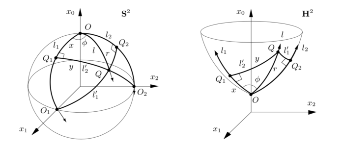
Figure 1: Ambient $(x_{0},x_{1},x_{2})$, geodesic parallel $(x,y)$ and geodesic polar $(r,\phi)$ coordinates of a point $Q$ on the sphere ${\mathbf{S}}^{2}$ with $\kappa=+1$ and on the hyperbolic space ${\mathbf{H}}^{2}$ with $\kappa=-1$ and $x_{0}\geq 1$. The origin of the space in ambient coordinates is $O=(1,0,0)$. Note that on ${\mathbf{S}}^{2}$, $O_{1}=(0,1,0)$ and $O_{2}=(0,0,1)$

3 Beltrami coordinates and projective dynamics

The quotients $(x_{1}/x_{0},x_{2}/x_{0})\equiv(q_{1},q_{2})$ of the ambient coordinates (8) are just the Beltrami coordinates of projective geometry for the sphere and the hyperbolic plane. They are obtained by applying the central stereographic projection with pole $(0,0,0)\in\mathbb{R}^{3}$ of a point $Q=(x_{0},x_{1},x_{2})$ onto the projective plane with $x_{0}=1$ and coordinates $(q_{1},q_{2})$:

$$(x_{0},x_{1},x_{2})\in\Sigma_{\kappa}\ \to\ (0,0,0)+\mu\,(1,q_{1},q_{2})\in\Sigma_{\kappa},$$

giving rise to the expressions

$$x_{0} =\mu=\frac{1}{\sqrt{1+\kappa(q_{1}^{2}+q_{2}^{2})}},\qquad x_{i}=\mu\,q_{i}=\frac{q_{i}}{\sqrt{1+\kappa(q_{1}^{2}+q_{2}^{2})}},$$ (18)

$$q_{i} =\frac{x_{i}}{x_{0}},\qquad q_{1}^{2}+q_{2}^{2}=\frac{1-x_{0}^{2}}{\kappa x_{0}^{2}},\qquad i=1,2.$$

Thus the origin $O=(1,0,0)\in\Sigma_{\kappa}$ goes to the origin $(q_{1},q_{2})=(0,0)$ in the projective space ${\mathbf{S}}^{2}_{\kappa}$.

The domain of $(q_{1},q_{2})$ depends on the value of the curvature $\kappa$. We write $\kappa$ in terms of the radius $R$ of the space as $\kappa=\pm 1/R^{2}$ and we find that in the sphere ${\mathbf{S}}^{2}$ with $\kappa=1/R^{2}>0$, $q_{i}\in(-\infty,+\infty)$. The points in the equator in $\Sigma_{\kappa}$ with $x_{0}=0$ ($x_{1}^{2}+x_{2}^{2}=R^{2}$) go to infinity, so that the projection (18) is well-defined for the hemisphere with $x_{0}>0$. In the hyperbolic or Lobachevski space ${\mathbf{H}}^{2}$ with $\kappa=-1/R^{2}<0$ and $x_{0}\geq 1$ it is satisfied that

$$q_{1}^{2}+q_{2}^{2}=\frac{x_{0}^{2}-1}{|\kappa|x_{0}^{2}}<R^{2},$$

which is the Poincaré disk in Beltrami coordinates and

$$q_{i}\in\bigl{(}-1/\sqrt{|\kappa|},+1/\sqrt{|\kappa|}\bigr{)}=\left(-R,+R\right).$$

The points at the infinity in ${\mathbf{H}}^{2}$ $(x_{0}\to\infty)$ are mapped onto to the circle $q_{1}^{2}+q_{2}^{2}=R^{2}$. Finally, in the Euclidean plane ${\mathbf{E}}^{2}$, with $\kappa=0$ ($R\to\infty$), the Beltrami coordinates are just the Cartesian ones $x_{i}=q_{i}\in(-\infty,+\infty)$.

By introducing (18) in the ambient metric (9) and in the free Lagrangian (12) we obtain that

$$({\rm d}s)_{\kappa}^{2}=\frac{(1+\kappa\,{\mathbf{q}}^{2}){\rm d}{\mathbf{q}}^{2}-\kappa({\mathbf{q}}\cdot{\rm d}{\mathbf{q}})^{2}}{(1+\kappa\,{\mathbf{q}}^{2})^{2}},\quad{\cal L}_{\kappa}=\frac{(1+\kappa\,{\mathbf{q}}^{2})\dot{{\mathbf{q}}}^{2}-\kappa({\mathbf{q}}\cdot\dot{{\mathbf{q}}})^{2}}{2(1+\kappa\,{\mathbf{q}}^{2})^{2}},$$ (19)

where ${\mathbf{q}}=(q_{1},q_{2})$ and hereafter we shall use the following notation for any 2-vectors ${\mathbf{a}}=(a_{1},a_{2})$ and ${\mathbf{b}}=(b_{1},b_{2})$:

$${\mathbf{a}}^{2}=a_{1}^{2}+a_{2}^{2},\qquad{\mathbf{a}}\cdot{\mathbf{b}}=a_{1}b_{1}+a_{2}b_{2}.$$

The Beltrami momenta ${\mathbf{p}}=(p_{1},p_{2})$ conjugate to the coordinates ${\mathbf{q}}$, such that $\{q_{i},p_{j}\}=\delta_{ij}$, come from $p_{i}=\partial{\cal L}_{\kappa}/\partial\dot{q}_{i}$

$$p_{i}=\frac{(1+\kappa\,{\mathbf{q}}^{2})\dot{q}_{i}-\kappa({\mathbf{q}}\cdot{\dot{{\mathbf{q}}}})q_{i}}{(1+\kappa\,{\mathbf{q}}^{2})^{2}},\qquad\dot{q}_{i}=(1+\kappa\,{\mathbf{q}}^{2})\bigl{(}p_{i}+\kappa({\mathbf{q}}\cdot{{{\mathbf{p}}}})q_{i}\bigr{)}.$$ (20)

And by inserting these expressions into ${\cal L}_{\kappa}$ (19) we get the free Hamiltonian

$${\cal T}_{\kappa}=\tfrac{1}{2}(1+\kappa\,{\mathbf{q}}^{2})\bigl{(}{\mathbf{p}}^{2}+\kappa({\mathbf{q}}\cdot{{{\mathbf{p}}}})^{2}\bigr{)}.$$ (21)

By introducing (18) and (20) in (13) we obtain the ambient momenta written in terms of the Beltrami variables, $\pi_{\mu}({\mathbf{q}},{\mathbf{p}})$, and from this result a symplectic realization of the Lie–Poisson generators (11) in these variables is directly found. These expressions are displayed in Table 1. Notice that the kinetic energy (21) can also be recovered by computing the symplectic realization of the Casimir (3) of $\mathfrak{so}_{\kappa}(3)$ in Beltrami variables as ${\mathcal{T}}_{\kappa}\equiv\frac{1}{2}{\mathcal{C}}$. Likewise the ambient momenta $\pi_{\mu}$ and symplectic realization of the Lie–Poisson generators $J_{\mu\nu}$ can be computed in the geodesic variables introduced in Section 2.2, and these are also presented in Table 1.

We recall that a similar procedure can be performed with Poincaré coordinates [37] which come from the stereographic projection with pole $(-1,0,0)$. The resulting expressions can be found in [32].

Table 1: Expressions for the ambient variables $(x_{\mu},\pi_{\mu})$, free Hamiltonian ${\cal T}_{\kappa}$ and symplectic realization of the Lie–Poisson generators $J_{\mu\nu}$ of $\mathfrak{so}_{\kappa}(3)$ in terms of Beltrami, geodesic parallel and geodesic polar canonical variables. The specific expressions for ${\mathbf{S}}^{2}$, ${\mathbf{H}}^{2}$ and ${\mathbf{E}}^{2}$ correspond to set $\kappa>0$, $\kappa<0$ and $\kappa=0$, respectively

	Beltrami $({\mathbf{q}},{\mathbf{p}})$	Geodesic parallel $(x,y,p_{x},p_{y})\qquad$	Geodesic polar $(r,\phi,p_{r},p_{\phi})$
$x_{0}$	$\displaystyle{\frac{1}{({1+\kappa{\mathbf{q}}^{2}})^{1/2}}}$	${\rm\ \!C}_{\kappa}(x){\rm\ \!C}_{\kappa}(y)$	${\rm\ \!C}_{\kappa}(r)$
$x_{1}$	$\displaystyle{\frac{q_{1}}{({1+\kappa{\mathbf{q}}^{2}})^{1/2}}}$	${\rm\ \!S}_{\kappa}(x){\rm\ \!C}_{\kappa}(y)$	${\rm\ \!S}_{\kappa}(r)\cos\phi$
$x_{2}$	$\displaystyle{\frac{q_{2}}{({1+\kappa{\mathbf{q}}^{2}})^{1/2}}}$	${\rm\ \!S}_{\kappa}(y)$	${\rm\ \!S}_{\kappa}(r)\sin\phi$
$\pi_{0}$	$\displaystyle{-\sqrt{1+\kappa{\mathbf{q}}^{2}}\,({\mathbf{q}}\cdot{\mathbf{p}})}$	$\displaystyle{-\frac{{\rm\ \!S}_{\kappa}(x)}{{\rm\ \!C}_{\kappa}(y)}\,p_{x}-{\rm\ \!C}_{\kappa}(x){\rm\ \!S}_{\kappa}(y)p_{y}}$	$-{\rm\ \!S}_{\kappa}(r)\,p_{r}$
$\pi_{1}$	$\displaystyle{\sqrt{1+\kappa{\mathbf{q}}^{2}}\,p_{1}}$	$\displaystyle{\frac{{\rm\ \!C}_{\kappa}(x)}{{\rm\ \!C}_{\kappa}(y)}\,p_{x}-\kappa{\rm\ \!S}_{\kappa}(x){\rm\ \!S}_{\kappa}(y)p_{y}}$	$\displaystyle{{\rm\ \!C}_{\kappa}(r)\cos\phi\,p_{r}-\frac{\sin\phi}{{\rm\ \!S}_{\kappa}(r)}\,p_{\phi}}$
$\pi_{2}$	$\displaystyle{\sqrt{1+\kappa{\mathbf{q}}^{2}}\,p_{2}}$	$\displaystyle{{\rm\ \!C}_{\kappa}(y)p_{y}}$	$\displaystyle{{\rm\ \!C}_{\kappa}(r)\sin\phi\,p_{r}+\frac{\cos\phi}{{\rm\ \!S}_{\kappa}(r)}\,p_{\phi}}$
${\cal T}_{\kappa}$	$\displaystyle{\frac{1}{2}(1+\kappa{\mathbf{q}}^{2})({\mathbf{p}}^{2}+\kappa({\mathbf{q}}\cdot{\mathbf{p}})^{2})}\quad$	$\displaystyle{\frac{1}{2}\left(\frac{p_{x}^{2}}{{\rm\ \!C}_{\kappa}^{2}(y)}+p_{y}^{2}\right)}$	$\displaystyle{\frac{1}{2}\left(p_{r}^{2}+\frac{p_{\phi}^{2}}{{\rm\ \!S}_{\kappa}^{2}(r)}\right)}$
$J_{01}$	$\displaystyle{p_{1}+\kappa({\mathbf{q}}\cdot{\mathbf{p}})q_{1}}$	$\displaystyle{p_{x}}$	$\displaystyle{\cos\phi\,p_{r}-\frac{\sin\phi}{{\rm\ \!T}_{\kappa}(r)}\,p_{\phi}}$
$J_{02}$	$\displaystyle{p_{2}+\kappa({\mathbf{q}}\cdot{\mathbf{p}})q_{2}}$	$\displaystyle{{\rm\ \!C}_{\kappa}(x)p_{y}+\kappa{\rm\ \!S}_{\kappa}(x){\rm\ \!T}_{\kappa}(y)p_{x}}$	$\displaystyle{\sin\phi\,p_{r}+\frac{\cos\phi}{{\rm\ \!T}_{\kappa}(r)}\,p_{\phi}}$
$J_{12}$	$\displaystyle{q_{1}p_{2}-q_{2}p_{1}}$	$\displaystyle{{\rm\ \!S}_{\kappa}(x)p_{y}-{\rm\ \!C}_{\kappa}(x){\rm\ \!T}_{\kappa}(y)p_{x}}$	$\displaystyle{p_{\phi}}$

4 Anisotropic oscillators on the Euclidean plane

To start with, let us consider the Hamiltonian determining the anisotropic oscillator with unit mass and frequencies $\omega_{x}$ and $\omega_{y}$ on the Euclidean plane in Cartesian coordinates $(x,y)\in\mathbb{R}^{2}$ and conjugate momenta $(p_{x},p_{y})$:

$${H}=\frac{1}{2}(p_{x}^{2}+p_{y}^{2})+\frac{1}{2}(\omega_{x}^{2}x^{2}+\omega_{y}^{2}y^{2}).$$ (22)

Clearly, this Hamiltonian is always integrable due to its separability in Cartesian coordinates so that it Poisson-commutes with the (quadratic in the momenta) integrals of motion

$${I}_{x}=\frac{1}{2}p_{x}^{2}+\frac{1}{2}\omega_{x}^{2}x^{2},\qquad{I}_{y}=\frac{1}{2}p_{y}^{2}+\frac{1}{2}\omega_{y}^{2}y^{2},$$

which are not independent since

$${H}={I}_{x}+{I}_{y}.$$

Furthermore, it is also well-known that for commensurate frequencies $\omega_{x}:\omega_{y}$ the Hamiltonian (22) provides a superintegrable system [38, 39, 40], in such a manner that an “additional” (in general higher-order in the momenta) integral of motion does exist.

The (super)integrability properties of the commensurate oscillator will be sketched by following the approach given in [41, 42], which is based on a classical factorization formalism (see [43, 44, 45, 46, 47] and references therein). If we denote

$$\omega_{x}=\gamma\omega_{y},\qquad\omega_{y}=\omega,\qquad\gamma\in\mathbb{R}^{+}/\{0\},$$ (23)

then $H$ (22) can be written in terms of the parameter $\gamma$ and frequency $\omega$ as

$$H=\frac{1}{2}(p_{x}^{2}+p_{y}^{2})+\frac{\omega^{2}}{2}\left((\gamma x)^{2}+y^{2}\right).$$ (24)

Next we introduce new canonical variables

$$\xi=\gamma x,\qquad p_{\xi}=p_{x}/\gamma,\qquad\xi\in\mathbb{R},$$ (25)

giving rise to

$$H=\frac{1}{2}\,p_{y}^{2}+\frac{\omega^{2}}{2}\,y^{2}+\gamma^{2}\left(\frac{1}{2}\,p_{\xi}^{2}+\frac{\omega^{2}}{2\gamma^{2}}\,\xi^{2}\right).$$ (26)

Therefore we obtain two 1D Hamiltonians $H^{\xi}$ and $H^{y}$ given by

$$H^{\xi}=\frac{1}{2}\,p_{\xi}^{2}+\frac{\omega^{2}}{2\gamma^{2}}\xi^{2},\qquad H^{y}=\frac{1}{2}\,p_{y}^{2}+\frac{\omega^{2}}{2}y^{2},\qquad H=H^{y}+\gamma^{2}H^{\xi},$$ (27)

which are two integrals of the motion for $H$. The 1D Hamiltonian $H^{\xi}$ (27) can then be factorized in terms of “ladder functions” $B^{\pm}$ as

$$H^{\xi}=B^{+}B^{-},\qquad B^{\pm}={\mp}\frac{i}{\sqrt{2}}\,p_{\xi}+\frac{1}{\sqrt{2}}\frac{\omega}{\gamma}\,\xi\,,$$ (28)

fulfilling

$$\{H^{\xi},B^{\pm}\}=\mp i\,\frac{\omega}{\gamma}\,B^{\pm},\qquad\{B^{-},B^{+}\}=-i\,\frac{\omega}{\gamma}.$$

The remaining 1D Hamiltonian $H^{y}$ (27) can also be factorized through “shift functions” $A^{\pm}$ in the form

$$H^{y}=A^{+}A^{-},\qquad A^{\pm}=\mp\frac{i}{\sqrt{2}}\,p_{y}-\frac{\omega}{\sqrt{2}}\,y\,,$$ (29)

so that

$$\{H^{y},A^{\pm}\}=\pm i{\omega}A^{\pm},\qquad\{A^{-},A^{+}\}=i{\omega}.$$

Notice that the sets of functions $(H^{\xi},B^{\pm},1)$ and $(H^{y},A^{\pm},1)$ span a Poisson–Lie algebra isomorphic to the harmonic oscillator Lie algebra $\mathfrak{h}_{4}$. Hence, the 2D Hamiltonian (26) can finally be expressed in terms of the above ladder and shift functions as

$$H=A^{+}A^{-}+\gamma^{2}B^{+}B^{-},\qquad\{H,B^{\pm}\}=\mp i{\gamma}{\omega}B^{\pm},\qquad\{H,A^{\pm}\}=\pm{i\omega}A^{\pm}\,.$$

The remarkable fact now is that if we consider a rational value for $\gamma$,

$$\gamma=\frac{\omega_{x}}{\omega_{y}}=\frac{m}{n},\qquad m,n\in\mathbb{N}^{\ast},$$ (30)

we obtain two additional complex constants of the motion $X^{\pm}$ for $H$ (26)

$$X^{\pm}=(B^{\pm})^{n}(A^{\pm})^{m}\,,\qquad\bar{X}^{+}={X}^{-},$$ (31)

which are of $(m+n)$th-order in the momenta. Real-valued integrals of the motion can be defined through the expressions

$$X=\frac{1}{2}(X^{+}+X^{-}),\qquad Y=\frac{1}{2i}(X^{+}-X^{-}).$$ (32)

The final result can be summarized as follows [41, 42].

1. The Hamiltonian $H$ (26) is always integrable for any value of the real parameter $\gamma$, since it is endowed with a quadratic constant of the motion given by either $H^{\xi}$ or $H^{y}$ (27).
   

2. When $\gamma=m/n$ is a rational parameter (30), the Hamiltonian (26) defines a superintegrable anisotropic oscillator with commensurate frequencies $\omega_{x}:\omega_{y}$ and the additional constant of the motion is given by either $X$ or $Y$ in (32). The sets $(H,H^{\xi},X)$ and $(H,H^{\xi},Y)$ are formed by three functionally independent functions.
   

3. When $(m+n)$ is even, the highest order constant of the motion in the momenta is $X$ being of $(m+n)$-degree, while $Y$ is of lower order $(m+n-1)$. When $(m+n)$ is odd, the highest $(m+n)$-degree integral is $Y$ while $X$ is of lower order $(m+n-1)$.

It is worth recalling that the Hamiltonian (22) can be enlarged by adding two Rosochatius (or Smorodinski-Winternitz) terms as

$${H}_{\lambda}=\frac{1}{2}(p_{x}^{2}+p_{y}^{2})+\frac{1}{2}(\omega_{x}^{2}x^{2}+\omega_{y}^{2}y^{2})+\frac{\lambda_{1}}{x^{2}}+\frac{\lambda_{2}}{y^{2}},$$ (33)

where $\lambda_{1}$ and $\lambda_{2}$ are real parameters, which provide centrifugal barriers when both constants are positive ones. In the 3D case, the resulting Hamiltonian, called “caged anisotropic oscillator”, has been solved in [48] (for both classical and quantum systems), and the general $N$D case has been fully studied in [40]. Despite the introduction of the $\lambda_{i}$-potentials, the Hamiltonian (33) is again (maximally) superintegrable for commensurate frequencies (in any dimension).

We also remark that any $m:n$ oscillator (labelled by $\gamma$) is equivalent to the $n:m$ one (with $1/\gamma$) via the interchanges $x\leftrightarrow y$ and $\gamma\omega\leftrightarrow\omega$. Consequently, according to the above statement the only anisotropic oscillators which are quadratically superintegrable correspond to the cases with $\gamma=1$ and $\gamma=2$ (so also $\gamma=1/2$), in agreement with the classifications on superintegrable Euclidean systems given in [7, 49, 50]. In the sequel, we will illustrate the previous general results by working out these two particular cases.

4.1 The $\gamma=1$ or 1:1 (isotropic) oscillator

We set $m=n=1$ so that the relations (23) and (25) simply give $\omega_{x}=\omega_{y}=\omega$ and $\xi=x$ and $p_{\xi}=p_{x}$. Thus we recover the isotropic oscillator

$${H}^{1:1}=\frac{1}{2}(p_{x}^{2}+p_{y}^{2})+\frac{\omega^{2}}{2}(x^{2}+y^{2}),$$ (34)

and the constants of the motion (32) reduce to

$$X=-\tfrac{1}{2}(p_{x}p_{y}+\omega^{2}xy),\qquad Y=-\tfrac{1}{2}\omega(xp_{y}-yp_{x}).$$ (35)

Since $(m+n)=2$ is even, we find a quadratic integral $X$, which is one of the components of the Demkov–Fradkin tensor [51, 52], and a first-order one $Y$ which is proportional to the angular momentum

$$\mathcal{J}=xp_{y}-yp_{x}.$$ (36)

We recall that if we add the two “centrifugal” $\lambda_{i}$-terms (33), then we get the 2D version of the so-called Smorodinsky–Winternitz system [53] which has been widely studied (see, e.g., [12, 15, 50, 54, 55, 56] and references therein).

4.2 The $\gamma=2$ or 2:1 oscillator

If we take $m=2$ and $n=1$, then $\omega_{x}=2\omega_{y}=2\omega$, $\xi=2x$ and $p_{\xi}=p_{x}/2$. The Hamiltonian (26) and the integrals (32) turn out to be

$$H^{2:1}=\frac{1}{2}\,p_{y}^{2}+\frac{\omega^{2}}{2}\,y^{2}+4\left(\frac{1}{2}\,p_{\xi}^{2}+\frac{\omega^{2}}{8}\,\xi^{2}\right)=\frac{1}{2}(p_{x}^{2}+p_{y}^{2})+\frac{\omega^{2}}{2}\left(4x^{2}+y^{2}\right),$$

$$X=-\frac{\omega}{4\sqrt{2}}\left(p_{y}(\xi p_{y}-4yp_{\xi})-\omega^{2}\xi y^{2}\right)=-\frac{\omega}{2\sqrt{2}}\left(p_{y}\mathcal{J}-\omega^{2}xy^{2}\right),$$ (37)

$$Y=\frac{1}{2\sqrt{2}}\left(p_{\xi}p_{y}^{2}+\omega^{2}y(\xi p_{y}-yp_{\xi})\right)=\frac{1}{4\sqrt{2}}\left(p_{x}p_{y}^{2}+\omega^{2}y(4xp_{y}-yp_{x})\right).$$

In this case $(m+n)=3$ is odd, so that we find a cubic integral $Y$ and a quadratic one $X$, which involves the angular momentum $\mathcal{J}$ (36); the latter is the integral of the motion which is usually considered in the literature (see e.g. [7, 57]) and shows that the 2:1 oscillator can be regarded as a superintegrable system with quadratic constants of the motion.

Notice that if we add a single Rosochatius-Winternitz potential $\lambda_{2}/y^{2}$ (by setting $\lambda_{1}=0$) the generalized system remains quadratically superintegrable [7], but if both $\lambda_{i}$-terms are introduced, the additional integral turns out to be of sixth-order in the momenta [40].

5 Anisotropic oscillators on ${{\mathbf{S}}}^{2}$ and ${{\mathbf{H}}}^{2}$

Let us recall that the classification of all possible superintegrable systems on ${\mathbf{S}}^{2}$ and ${\mathbf{H}}^{2}$ with quadratic integrals of the motion was performed in [7], where two curved superintegrable oscillator potentials were found:

• The isotropic Higgs oscillator [58], whose Euclidean limit is the 1:1 isotropic oscillator (34).
  

• The curved version of the superintegrable Euclidean 2:1 oscillator (37).

The aim of this Section is to present the construction of the constant-curvature Hamiltonian analogue $H_{\kappa}$ of the anisotropic Euclidean Hamiltonian $H$ (24) with arbitrary commensurate frequencies. The idea is to introduce appropriately the curvature parameter $\kappa$ by requiring to keep the same (super)integrability properties as given in the previous Section for (24) (or (26)) and, simultaneously, allowing for a smooth and well-defined flat limit $\kappa\to 0$ of the curved Hamiltonian and its constants of the motion.

This result has been achieved in [41] by using the geodesic parallel variables described in Section 2.2, so with kinetic term ${\cal T}_{\kappa}$ given by (16). Explicitly, the curved Hamiltonian ${H}_{\kappa}$ has been shown to be of the form

$${H}_{\kappa}={\cal T}_{\kappa}+{U}^{\gamma}_{\kappa}=\frac{1}{2}\left(\frac{p_{x}^{2}}{{\rm\ \!C}_{\kappa}^{2}(y)}+p_{y}^{2}\right)+\frac{\omega^{2}}{2}\left(\frac{{\rm\ \!T}_{\kappa}^{2}(\gamma x)}{{\rm\ \!C}_{\kappa}^{2}(y)}+{\rm\ \!T}_{\kappa}^{2}(y)\right).$$ (38)

By taking into account (17) and the presence of the $\kappa$-tangent ${\rm\ \!T}_{\kappa}(\gamma x)$ in the potential ${U}^{\gamma}_{\kappa}$, we find that the domain of the geodesic parallel coordinates $(x,y)$ is restricted to

$${\mathbf{S}}^{2}\ (\kappa>0): -\frac{\pi}{2\sqrt{\kappa}}<\gamma x<\frac{\pi}{2\sqrt{\kappa}},\quad-\frac{\pi}{2\sqrt{\kappa}}<y<\frac{\pi}{2\sqrt{\kappa}},\quad\gamma\geq\frac{1}{2}.$$

$${\mathbf{H}}^{2}\ (\kappa<0): x,y\in\mathbb{R},\quad\gamma\in\mathbb{R}^{+}/\{0\}.$$

Now we assume that $\kappa\neq 0$ and since $1+\kappa{\rm\ \!T}_{\kappa}^{2}(u)=1/{\rm\ \!C}_{\kappa}^{2}(u)$ we rewrite the Hamiltonian ${H}_{\kappa}$ (38) as

$$H_{\kappa}=\frac{p_{y}^{2}}{2}+\frac{1}{{\rm\ \!C}_{\kappa}^{2}(y)}\left(\frac{p_{x}^{2}}{2}+\frac{\omega^{2}}{2\kappa{\rm\ \!C}_{\kappa}^{2}(\gamma x)}\right)-\frac{\omega^{2}}{2\kappa},\qquad\kappa\neq 0.$$ (39)

Next we introduce the canonical variables $(\xi,p_{\xi})$ (25) finding that

$$H_{\kappa}=\frac{p_{y}^{2}}{2}+\frac{\gamma^{2}}{{\rm\ \!C}_{\kappa}^{2}(y)}\left(\frac{p_{\xi}^{2}}{2}+\frac{\omega^{2}}{2\kappa\gamma^{2}{\rm\ \!C}_{\kappa}^{2}(\xi)}\right)-\frac{\omega^{2}}{2\kappa}\,,\qquad\kappa\neq 0.$$

And the curved Hamiltonian (39) is finally expressed as

$$H_{\kappa}=\frac{p_{y}^{2}}{2}+\frac{\gamma^{2}H_{\kappa}^{\xi}}{{\rm\ \!C}_{\kappa}^{2}(y)}-\frac{\omega^{2}}{2\kappa},\qquad H_{\kappa}^{\xi}=\frac{p_{\xi}^{2}}{2}+\frac{\omega^{2}}{2\kappa\gamma^{2}{\rm\ \!C}_{\kappa}^{2}(\xi)},\qquad\kappa\neq 0,$$ (40)

where $H_{\kappa}^{\xi}$ is a constant of the motion. Notice that in this form, the 1D Hamiltonians $H_{\kappa}^{\xi}$ and $H_{\kappa}$ correspond to Pöschl–Teller systems [44]. Consequently, $H_{\kappa}$ determines an integrable system for any value of $\omega$ and $\gamma$.

In the sequel, we factorize the 1D Hamiltonians $H_{\kappa}^{\xi}$ and $H_{\kappa}$ (40) (see [42, 41, 44] for details). By one hand, the Hamiltonian $H_{\kappa}^{\xi}$ is factorized in terms of ladder functions as

$$H_{\kappa}^{\xi}=B_{\kappa}^{+}B_{\kappa}^{-}+\frac{\omega^{2}}{2\kappa\gamma^{2}},\qquad B_{\kappa}^{\pm}={\mp}\frac{i}{\sqrt{2}}{\rm\ \!C}_{\kappa}(\xi)\,p_{\xi}+\frac{\mathcal{E}_{\kappa}}{\sqrt{2}}{\rm\ \!S}_{\kappa}(\xi),$$ (41)

where $\mathcal{E}_{\kappa}$ is a constant of the motion defined by

$$\mathcal{E}_{\kappa}(p_{\xi},\xi):=\sqrt{2\kappa H_{\kappa}^{\xi}}\,.$$ (42)

Thus we get the Poisson algebra

$$\{H_{\kappa}^{\xi},B_{\kappa}^{\pm}\}=\mp i\,\mathcal{E}_{\kappa}\,B_{\kappa}^{\pm},\qquad\{B_{\kappa}^{-},B_{\kappa}^{+}\}=-i\,\mathcal{E}_{\kappa}\,,$$

so that

$$\{H_{\kappa},B_{\kappa}^{\pm}\}=\mp i\,\frac{\gamma^{2}\mathcal{E}_{\kappa}}{{\rm\ \!C}_{\kappa}^{2}(y)}\,B_{\kappa}^{\pm}.$$

On the other hand, $H_{\kappa}$ is factorized by means of shift functions in the form

$$H_{\kappa}=A_{\kappa}^{+}A_{\kappa}^{-}+\frac{1}{2\kappa}\left(\gamma^{2}\mathcal{E}_{\kappa}^{2}-\omega^{2}\right),\qquad A_{\kappa}^{\pm}=\mp\frac{i}{\sqrt{2}}\,p_{y}-\frac{\gamma\mathcal{E}_{\kappa}}{\sqrt{2}}{\rm\ \!T}_{\kappa}(y),$$ (43)

closing on the Poisson algebra

$$\{H_{\kappa},A_{\kappa}^{\pm}\}=\pm i\,\frac{\gamma\mathcal{E}_{\kappa}}{{\rm\ \!C}_{\kappa}^{2}(y)}\,A_{\kappa}^{\pm},\qquad\{A_{\kappa}^{-},A_{\kappa}^{+}\}=i\,\frac{\gamma\mathcal{E}_{\kappa}}{{\rm\ \!C}^{2}_{\kappa}(y)}.$$

As in the Euclidean case, when $\gamma$ takes a rational value (30), two additional complex integrals of motion arise for $H_{\kappa}$ (38) (under the change of variable (25)), namely

$$X_{\kappa}^{\pm}=(B_{\kappa}^{\pm})^{n}(A_{\kappa}^{\pm})^{m},\qquad\bar{X}_{\kappa}^{+}={X}_{\kappa}^{-}.$$ (44)

Nevertheless, in order to obtain real constants of the motion, $X_{\kappa}$ and $Y_{\kappa}$, we are now led to distinguish between two situations [47] (due to the presence of powers of $\mathcal{E}_{\kappa}$ (42) in (44)):

$$\mbox{When $m+n$ is even:}\quad X_{\kappa}^{\pm}=\pm i\,\mathcal{E}_{\kappa}Y_{\kappa}+X_{\kappa}.$$ (45)

$$\mbox{When $m+n$ is odd:}\quad X_{\kappa}^{\pm}=\mathcal{E}_{\kappa}X_{\kappa}\pm i\,Y_{\kappa}.$$

Summing up, the generalization to $\mathbf{S}^{2}$ and $\mathbf{H}^{2}$ of the anisotropic oscillator can be stated as follows [41].

1. For any value of $\gamma$, the Hamiltonian $H_{\kappa}$ (38) always determines an integrable anisotropic curved oscillator on ${\mathbf{S}}^{2}$ and ${\mathbf{H}}^{2}$, with quadratic constant of motion given by $H^{\xi}_{\kappa}$ (40).
   

2. When $\gamma$ is a rational parameter (30), the Hamiltonian $H_{\kappa}$ defines a superintegrable anisotropic curved oscillator and the additional constant of the motion is given by either $X_{\kappa}$ or $Y_{\kappa}$ in (45). The sets $(H_{\kappa},H_{\kappa}^{\xi},X_{\kappa})$ and $(H_{\kappa},H_{\kappa}^{\xi},Y_{\kappa})$ are formed by three functionally independent functions.
   

3. The integrals $X_{\kappa}$ and $Y_{\kappa}$ are polynomial in the momenta, whose degrees are $(m+n)$ and $(m+n-1)$ when $(m+n)$ is even, and $(m+n-1)$ and $(m+n)$ when $(m+n)$ is odd, respectively.

Some remarks are in order. Firstly, although the (flat) Euclidean limit $\kappa\to 0$ is precluded for $H_{\kappa}$ written in the forms (39) and (40), it is actually well-defined in all the remaining expressions. To perform the contractions one has to take into account the following flat limit of the integrals $H_{\kappa}^{\xi}$ (40) and $\mathcal{E}_{\kappa}$ (42)

$$\lim_{\kappa\to 0}\kappa H_{\kappa}^{\xi}=\frac{\omega^{2}}{2\gamma^{2}},\qquad\lim_{\kappa\to 0}\mathcal{E}_{\kappa}=\frac{\omega}{\gamma}.$$ (46)

Therefore, it can be easily checked that when $\kappa\to 0$, the curved Hamiltonian $H_{\kappa}$ (38) reduce to $H$ (24), the curved ladder functions $B_{\kappa}^{\pm}$ (41) to $B^{\pm}$ (28), the curved shift functions $A_{\kappa}^{\pm}$ (43) to $A^{\pm}$ (29), and so the curved integrals $X_{\kappa}^{\pm}$ (44) to $X^{\pm}$ (31).

Secondly, as in the Euclidean system (33), the curved Hamiltonian $H_{\kappa}$ (38) can be generalized by adding two curved Rosochatius–Winternitz potentials which in ambient coordinates (15) adopt a very simple expression [12, 15]. Explicitly, the corresponding potential reads

$${U}^{\gamma}_{\kappa,\lambda}={U}^{\gamma}_{\kappa}+\frac{\lambda_{1}}{x_{1}^{2}}+\frac{\lambda_{2}}{x_{2}^{2}}=\left(\frac{{\rm\ \!T}_{\kappa}^{2}(\gamma x)}{{\rm\ \!C}_{\kappa}^{2}(y)}+{\rm\ \!T}_{\kappa}^{2}(y)\right)+\frac{\lambda_{1}}{{\rm\ \!S}^{2}_{\kappa}(x){\rm\ \!C}^{2}_{\kappa}(y)}+\frac{\lambda_{2}}{{\rm\ \!S}^{2}_{\kappa}(y)}.$$ (47)

Then the corresponding Hamiltonian ${H}_{\kappa,\lambda}={\cal T}_{\kappa}+{U}^{\gamma}_{\kappa,\lambda}$ can be written as (with $\kappa\neq 0$)

$${H}_{\kappa,\lambda}=\frac{p_{y}^{2}}{2}+\frac{\lambda_{2}}{{\rm\ \!S}^{2}_{\kappa}(y)}+\frac{1}{{\rm\ \!C}_{\kappa}^{2}(y)}\left(\frac{p_{x}^{2}}{2}+\frac{\omega^{2}}{2\kappa{\rm\ \!C}_{\kappa}^{2}(\gamma x)}+\frac{\lambda_{1}}{{\rm\ \!S}^{2}_{\kappa}(x)}\right)-\frac{\omega^{2}}{2\kappa},$$

to be compared with (39). Consequently, ${H}_{\kappa,\lambda}$ defines an integrable system for any value of $\omega$, $\gamma$, $\lambda_{1}$ and $\lambda_{2}$.

Now it could be expected that if $\gamma$ is a rational number, ${H}_{\kappa,\lambda}$ should be again superintegrable but, to the best of our knowledge, this property has not been proven in general (except for $\gamma=1$). We also point out that each $\lambda_{i}$-term gives rise to a centrifugal barrier on $\mathbf{H}^{2}$ when $\lambda_{i}>0$, as in the Euclidean system but, surprisingly enough, both $\lambda_{1}$- and $\lambda_{2}$-potentials can be interpreted as noncentral 1D curved oscillators on $\mathbf{S}^{2}$ with centres at the points $O_{1}=(0,1,0)$ and $O_{2}=(0,0,1)$, respectively [10, 11, 12, 13, 31, 59] (see Figure 1).

Thirdly, it can be seen from $H_{\kappa}$ (38) that, in general, $U_{\kappa}^{\gamma}$ and $U_{\kappa}^{1/\gamma}$ determine two different systems, in contradistinction with the Euclidean case (recall that the equivalence was provided by the interchanges $x\leftrightarrow y$ and $\gamma\omega\leftrightarrow\omega$). However when $\kappa=0$ both potentials reduce to equivalent Euclidean potentials. This clearly illustrates the fact that given a flat Hamiltonian system there could be not a single but several curved generalizations (or curvature integrable deformations) which would be non-equivalent in the sense that no canonical change of variables exist between them.

Fourthly, according to the results previously presented, the only anisotropic curved oscillators which are quadratically superintegrable correspond to the same values of $\gamma$ as in the Euclidean system [7, 60, 61]: $\gamma=1$, $\gamma=2$ and (now the non-equivalent) $\gamma=1/2$. In what follows we shall present the corresponding results for the these three cases.

And finally, we recall that other integrable anisotropic oscillators on the spheres and hyperbolic spaces can be found in [62, 63, 64, 65] (see also references therein).

5.1 The $\gamma=1$ or 1:1 curved (isotropic) oscillator

This case is also known as the Higgs oscillator [58, 66] and it has been widely studied in the literature (see [7, 16, 31, 67, 68, 69, 70] and references therein).

We set $\gamma=m=n=1$ so that $\xi=x$ and $p_{\xi}=p_{x}$. The Hamiltonian $H_{\kappa}$ (38) reduces to

$${H}_{\kappa}^{1:1}=\frac{1}{2}\left(\frac{p_{x}^{2}}{{\rm\ \!C}_{\kappa}^{2}(y)}+p_{y}^{2}\right)+\frac{\omega^{2}}{2}\left(\frac{{\rm\ \!T}_{\kappa}^{2}(x)}{{\rm\ \!C}_{\kappa}^{2}(y)}+{\rm\ \!T}_{\kappa}^{2}(y)\right)=\frac{p_{y}^{2}}{2}+\frac{H_{\kappa}^{x}}{{\rm\ \!C}_{\kappa}^{2}(y)}-\frac{\omega^{2}}{2\kappa},$$

where the quadratic integral $H_{\kappa}^{x}\equiv H_{\kappa}^{\xi}$ (40) is given by

$$H_{\kappa}^{x}=\frac{p_{x}^{2}}{2}+\frac{\omega^{2}}{2\kappa{\rm\ \!C}_{\kappa}^{2}(x)}.$$

Since $(m+n)=2$ is even the constants of the motion (45) read

$$X_{\kappa}=-\frac{1}{2}\left({\rm\ \!C}_{\kappa}(x)p_{x}p_{y}+\mathcal{E}_{\kappa}^{2}{\rm\ \!S}_{\kappa}(x){\rm\ \!T}_{\kappa}(y)\right),$$

$$Y_{\kappa}=-\frac{1}{2}\,\left({\rm\ \!S}_{\kappa}(x)p_{y}-{\rm\ \!C}_{\kappa}(x){\rm\ \!T}_{\kappa}(y)p_{x}\right).$$

The integral $Y_{\kappa}$ is proportional to the (curved) angular momentum $\mathcal{J}_{\kappa}$ which in geodesic parallel and polar variables is given by [7, 9]

$$\mathcal{J}_{\kappa}={\rm\ \!S}_{\kappa}(x)p_{y}-{\rm\ \!C}_{\kappa}(x){\rm\ \!T}_{\kappa}(y)p_{x}=p_{\phi}.$$

The flat limit $\kappa\to 0$ of all the above expressions leads to the results of the Euclidean isotropic oscillator given in Section 4.1. In particular, provided that $\mathcal{E}_{\kappa}\to\omega$ (46), the integrals $X_{\kappa}$, $\mathcal{E}_{\kappa}Y_{\kappa}$ and the curved angular momentum $\mathcal{J}_{\kappa}$ reduce to (35) and (36).

Notice that the potential of ${H}_{\kappa}^{1:1}$ is expressed in terms of ambient and geodesic polar coordinates (15) as

$${U}_{\kappa}^{1:1}=\frac{\omega^{2}}{2}\left(\frac{x_{1}^{2}+x_{2}^{2}}{x_{0}^{2}}\right)=\frac{\omega^{2}}{2}{\rm\ \!T}^{2}_{\kappa}(r).$$

If we consider the two $\lambda_{i}$-potentials (47), we recover the curved Smorodinsky–Winternitz system

$${U}_{\kappa,\lambda}^{1:1}=\frac{\omega^{2}}{2}\left(\frac{x_{1}^{2}+x_{2}^{2}}{x_{0}^{2}}\right)+\frac{\lambda_{1}}{x_{1}^{2}}+\frac{\lambda_{2}}{x_{2}^{2}},$$

which is known to be quadratically superintegrable [7, 12, 13, 15, 31, 71].

5.2 The $\gamma=2$ or 2:1 curved oscillator

We set $\gamma=m=2$ and $n=1$ so that $\xi=2x$ and $p_{\xi}=p_{x}/2$. The Hamiltonian $H_{\kappa}$ (38) reads

$${H}_{\kappa}^{2:1}=\frac{1}{2}\left(\frac{p_{x}^{2}}{{\rm\ \!C}_{\kappa}^{2}(y)}+p_{y}^{2}\right)+\frac{\omega^{2}}{2}\left(\frac{{\rm\ \!T}_{\kappa}^{2}(2x)}{{\rm\ \!C}_{\kappa}^{2}(y)}+{\rm\ \!T}_{\kappa}^{2}(y)\right)=\frac{p_{y}^{2}}{2}+\frac{4H_{\kappa}^{\xi}}{{\rm\ \!C}_{\kappa}^{2}(y)}-\frac{\omega^{2}}{2\kappa},$$

where

$$H_{\kappa}^{\xi}=\frac{p_{\xi}^{2}}{2}+\frac{\omega^{2}}{8\kappa{\rm\ \!C}_{\kappa}^{2}(\xi)}=\frac{p_{x}^{2}}{8}+\frac{\omega^{2}}{8\kappa{\rm\ \!C}_{\kappa}^{2}(2x)}.$$

Now $(m+n)=3$ is odd so that the constants of the motion (45) turn out to be

$$X_{\kappa}=-\frac{1}{2\sqrt{2}}\left(\left[{\rm\ \!S}_{\kappa}(2x)p_{y}-2{\rm\ \!C}_{\kappa}(2x){\rm\ \!T}_{\kappa}(y)p_{x}\right]p_{y}-4\mathcal{E}_{\kappa}^{2}{\rm\ \!S}_{\kappa}(2x){\rm\ \!T}^{2}_{\kappa}(y)\right),$$

$$Y_{\kappa}=\frac{1}{4\sqrt{2}}\left(\!{\rm\ \!C}_{\kappa}(2x)p_{x}p_{y}^{2}+4\mathcal{E}_{\kappa}^{2}{\rm\ \!T}_{\kappa}(y)\left[2{\rm\ \!S}_{\kappa}(2x)p_{y}-{\rm\ \!C}_{\kappa}(2x){\rm\ \!T}_{\kappa}(y)p_{x}\right]\right),$$

that is $X_{\kappa}$ is quadratic in the momenta, while $Y_{\kappa}$ is cubic; this means that ${H}_{\kappa}^{2:1}$ is a quadratically superintegrable system. The limit $\kappa\to 0$ (46) gives $\mathcal{E}_{\kappa}\to\omega/2$, hence the Hamiltonian ${H}_{\kappa}^{2:1}$ and the integrals $\mathcal{E}_{\kappa}X_{\kappa}$ and $Y_{\kappa}$ reduce to (37), thus reproducing the results of Section 4.2.

In terms of ambient and geodesic polar coordinates (15), the potential of ${H}_{\kappa}^{2:1}$ adopts the (cumbersome) expressions

$$\!\!\!{U}_{\kappa}^{2:1}=\frac{\omega^{2}}{2}\left(\frac{4x_{0}^{2}x_{1}^{2}}{(x_{0}^{2}+\kappa x_{1}^{2})(x_{0}^{2}-\kappa x_{1}^{2})^{2}}+\frac{x_{2}^{2}}{(1-\kappa x_{2}^{2})}\right)$$

$$\qquad=\frac{\omega^{2}}{2}\left(\frac{4{\rm\ \!T}^{2}_{\kappa}(r)\cos^{2}\phi}{\left(1-\kappa{\rm\ \!S}^{2}_{\kappa}(r)\sin^{2}\phi\right)\left(1-\kappa{\rm\ \!T}^{2}_{\kappa}(r)\cos^{2}\phi\right)^{2}}+\frac{{\rm\ \!S}^{2}_{\kappa}(r)\sin^{2}\phi}{1-\kappa{\rm\ \!S}^{2}_{\kappa}(r)\sin^{2}\phi}\right)$$

the latter is the one formerly introduced in [7].

In this case it is only possible to add a single $\lambda_{i}$-potential (47) keeping the quadratic superintegrability of the system [7]

$${U}_{\kappa,\lambda}^{2:1}={U}_{\kappa}^{2:1}+\frac{\lambda_{2}}{x_{2}^{2}},$$

which has been studied in detail in [31, 32]. In this respect, we remark that an equivalent superintegrable system can be obtained by interchanging the ambient coordinates $x_{1}\leftrightarrow x_{2}$ (so the role of the geodesics $l_{1}\leftrightarrow l_{2}$ in Section 2.2) which means that the geodesic parallel coordinates are mapped as $(x,y)\to(y^{\prime},x^{\prime})$, that is,

$$x_{0}={\rm\ \!C}_{\kappa}(x^{\prime}){\rm\ \!C}_{\kappa}(y^{\prime}),\qquad x_{1}={\rm\ \!S}_{\kappa}(x^{\prime}),\qquad x_{2}={\rm\ \!C}_{\kappa}(x^{\prime}){\rm\ \!S}_{\kappa}(y^{\prime}).$$

In fact, the coordinates $(x^{\prime},y^{\prime})$ are just the so-called geodesic parallel coordinates of type II [9]. These transformations provide the equivalent system

$${H^{\prime}}_{\kappa}^{2:1}={\cal T}_{\kappa}+\frac{\omega^{2}}{2}\left(\frac{x_{1}^{2}}{(1-\kappa x_{1}^{2})}+\frac{4x_{0}^{2}x_{2}^{2}}{(x_{0}^{2}+\kappa x_{2}^{2})(x_{0}^{2}-\kappa x_{2}^{2})^{2}}\right)$$

$$\qquad\quad=\frac{1}{2}\left(p_{x^{\prime}}^{2}+\frac{p_{y^{\prime}}^{2}}{{\rm\ \!C}_{\kappa}^{2}(x^{\prime})}\right)+\frac{\omega^{2}}{2}\left({\rm\ \!T}_{\kappa}^{2}(x^{\prime})+\frac{{\rm\ \!T}_{\kappa}^{2}(2y^{\prime})}{{\rm\ \!C}_{\kappa}^{2}(x^{\prime})}\right).$$ (48)

This is exactly the expression for the 2:1 curved oscillator considered in [31, 32].

5.3 The $\frac{1}{2}$:1 curved oscillator

We set $\gamma=1/2$, $m=1$ and $n=2$, so that $\xi=x/2$, $p_{\xi}=2p_{x}$. Thus the Hamiltonian $H_{\kappa}$ (38) is

$${H}_{\kappa}^{\frac{1}{2}:1}=\frac{1}{2}\left(\frac{p_{x}^{2}}{{\rm\ \!C}_{\kappa}^{2}(y)}+p_{y}^{2}\right)+\frac{\omega^{2}}{2}\left(\frac{{\rm\ \!T}_{\kappa}^{2}(\frac{x}{2})}{{\rm\ \!C}_{\kappa}^{2}(y)}+{\rm\ \!T}_{\kappa}^{2}(y)\right)=\frac{p_{y}^{2}}{2}+\frac{H_{\kappa}^{\xi}}{4{\rm\ \!C}_{\kappa}^{2}(y)}-\frac{\omega^{2}}{2\kappa}\,,$$

where

$$H_{\kappa}^{\xi}=\frac{p_{\xi}^{2}}{2}+\frac{2\omega^{2}}{\kappa{\rm\ \!C}_{\kappa}^{2}(\xi)}=2{p_{x}^{2}}+\frac{2\omega^{2}}{\kappa{\rm\ \!C}_{\kappa}^{2}(\frac{x}{2})}.$$

The sum $(m+n)=3$ is again odd, and the additional integrals (45) read

$$X_{\kappa}=-\frac{1}{4\sqrt{2}}\left(4\left[{\rm\ \!S}_{\kappa}(x)p_{y}-{\rm\ \!C}^{2}_{\kappa}(\tfrac{x}{2}){\rm\ \!T}_{\kappa}(y)p_{x}\right]p_{x}+\mathcal{E}_{\kappa}^{2}{\rm\ \!S}^{2}_{\kappa}(\tfrac{x}{2}){\rm\ \!T}_{\kappa}(y)\right),$$

$$Y_{\kappa}=\frac{1}{2\sqrt{2}}\left(4{\rm\ \!C}^{2}_{\kappa}(\tfrac{x}{2})p^{2}_{x}p_{y}-\mathcal{E}_{\kappa}^{2}\left[{\rm\ \!S}^{2}_{\kappa}(\tfrac{x}{2})p_{y}-{\rm\ \!S}_{\kappa}(x){\rm\ \!T}_{\kappa}(y)p_{x}\right]\right),$$

which shows that ${H}_{\kappa}^{\frac{1}{2}:1}$ is again a quadratically superintegrable system.

As a consequence, when both Hamiltonians ${H}_{\kappa}^{2:1}$ and ${H}_{\kappa}^{\frac{1}{2}:1}$ are considered altogether, one finds a particular issue where the curvature-deformation approach gives rise to two non-equivalent systems starting from the common “seed” given by the Euclidean system ${H}^{2:1}\simeq{H}^{\frac{1}{2}:1}$ (37) described in Section 4.2. Therefore, the plurality of possible integrable curved generalizations of a given Euclidean system becomes evident, and a deeper analysis of the curved system ${H}_{\kappa}^{\frac{1}{2}:1}$ seems to be needed, since –to the best of our knowledge– it has not been appropriately considered in the literature so far.

6 Integrable Hénon–Heiles systems

By making use of the results described in the previous Sections, our aim now will be to present the generalization to the 2D sphere and the hyperbolic space of the integrable Hénon–Heiles Hamiltonian given by

$$\mathcal{H}=\dfrac{1}{2}(p_{1}^{2}+p_{2}^{2})+\Omega\left(q_{1}^{2}+4q_{2}^{2}\right)+\alpha\left(q_{1}^{2}q_{2}+2q_{2}^{3}\right),$$ (49)

where $\Omega$ and $\alpha$ are real constants. Such curved Hénon–Heiles Hamiltonian will be constructed by considering it as an integrable cubic perturbation of the 1:2 anisotropic oscillator that we have introduced in the previous Section 5.2, in the form (48), although in this case projective Beltrami coordinates of Section 3 will be the ones that are naturally adapted to the construction of the curved system.

We recall that the original (non-integrable) Hénon–Heiles system

$${H}=\dfrac{1}{2}(p_{1}^{2}+p_{2}^{2})+\dfrac{1}{2}(q_{1}^{2}+q_{2}^{2})+\lambda\left(q_{1}^{2}q_{2}-\frac{1}{3}\,q_{2}^{3}\right),$$

was introduced in [72] in order to model a Newtonian axially-symmetric galactic system. When the following generalization containing adjustable parameters was studied

$$\mathcal{H}=\dfrac{1}{2}(p_{1}^{2}+p_{2}^{2})+\Omega_{1}q_{1}^{2}+\Omega_{2}q_{2}^{2}+\alpha\left(q_{1}^{2}q_{2}+\beta q_{2}^{3}\right),$$

it was found that the only Liouville-integrable members of this family of generalized Hénon–Heiles Hamiltonians were given by three specific choices of the real parameters $\Omega_{1}$, $\Omega_{2}$, $\alpha$ and $\beta$ (see [73, 74, 75, 76, 77, 78, 79, 80, 81, 82, 83, 84, 85]):

• The Sawada–Kotera system, given by $\beta=1/3$ and $\Omega_{1}=\Omega_{2}=\Omega$:

  $$\mathcal{H}=\dfrac{1}{2}(p_{1}^{2}+p_{2}^{2})+\Omega\left(q_{1}^{2}+q_{2}^{2}\right)+\alpha\left(q_{1}^{2}q_{2}+\frac{1}{3}q_{2}^{3}\right).$$ (50)

  This system is separable in rotated Euclidean coordinates, and therefore its integral of the motion is quadratic in the momenta.
  

• The Korteweg–de Vries (KdV) system, with $\beta=2$ and $(\Omega_{1},\Omega_{2})$ arbitrary parameters:

  $$\mathcal{H}=\dfrac{1}{2}(p_{1}^{2}+p_{2}^{2})+\Omega_{1}q_{1}^{2}+\Omega_{2}q_{2}^{2}+\alpha\left(q_{1}^{2}q_{2}+2q_{2}^{3}\right),$$ (51)

  which is separable in parabolic coordinates and has also a quadratic integral of the motion.
  

• The Kaup–Kuperschdmit system, with $\beta=16/3$ and $\Omega_{2}=16\Omega_{1}=16\Omega$:

  $$\mathcal{H}=\dfrac{1}{2}(p_{1}^{2}+p_{2}^{2})+\Omega\left(q_{1}^{2}+16q_{2}^{2}\right)+\alpha\left(q_{1}^{2}q_{2}+\frac{16}{3}q_{2}^{3}\right),$$ (52)

  whose integral is quartic in the momenta.

Hence the particular KdV case (51) arising when $\Omega_{2}=4\Omega_{1}$ gives the Hamiltonian (49) and this is connected to the so-called Ramani–Dorizzi–Grammaticos (RDG) series of integrable potentials [86, 87], which are just the polynomial potentials on the Euclidean plane that can be separated in parabolic coordinates and can freely be superposed by preserving integrability [78, 88]. Moreover, such separability in parabolic coordinates explains why a large collection of integrable rational perturbations can be added to the RDG potentials (see [88, 89, 90, 91, 92] and references therein).

In the sequel we review the main results concerning the flat KdV Hénon–Heiles Hamiltonian (51) with $\Omega_{2}=4\Omega_{1}$ along with its associated RDG potentials. And in the next Section 7 we will sketch its integrable curved analogue on the 2D sphere S² and the hyperbolic (or Lobachevski) space H² which was constructed in [93], together with the full curved counterpart of the integrable RDG series of potentials. The corresponding integrable perturbations of the curved KdV system can be found in [85].

6.1 An integrable KdV Hénon–Heiles system on the Euclidean plane

Le us consider the integrable (albeit non-superintegrable) Hamiltonian system (49) defined on E² whose constant of motion is quadratic in the momenta and given by

$$\mathcal{I}=p_{1}(q_{1}p_{2}-q_{2}p_{1})+q_{1}^{2}\left(2\Omega q_{2}+\dfrac{\alpha}{4}(q_{1}^{2}+4q_{2}^{2})\right).$$ (53)

This system can be regarded as an integrable cubic perturbation of the 1:2 oscillator with frequencies $(\omega,2\omega)$ once the identification $\omega^{2}=2\Omega$ is performed (see Section 4.2).

The potential functions included in both the Hamiltonian (49) and its invariant (53) are directly connected to the so-called RDG series of integrable potentials, which consists of the homogeneous polynomial potentials of degree $n$ given by [86, 87]

$$\mathcal{V}_{n}(q_{1},q_{2})=\sum\limits_{i=0}^{[\frac{n}{2}]}2^{n-2i}\dbinom{n-i}{i}q_{1}^{2i}q_{2}^{n-2i}\,,\qquad n=1,2,\dots$$

Namely, the four members of this family read

$$\mathcal{V}_{1}(q_{1},q_{2})=2q_{2},$$

$$\mathcal{V}_{2}(q_{1},q_{2})=q_{1}^{2}+4q_{2}^{2},$$

$$\mathcal{V}_{3}(q_{1},q_{2})=4q_{1}^{2}q_{2}+8q_{2}^{3},$$

$$\mathcal{V}_{4}(q_{1},q_{2})=q_{1}^{4}+12q_{1}^{2}q_{2}^{2}+16q_{2}^{4}.$$

It is straightforward to realize that the quadratic and cubic potentials in the Hamiltonian (49) are just the second- and the third-order RDG potentials $\mathcal{V}_{2}$ and $\mathcal{V}_{3}$, respectively. Moreover, the integral $\mathcal{I}$ (53) contains the linear $\mathcal{V}_{1}$ and the quadratic $\mathcal{V}_{2}$ RDG potentials. Therefore, the integrable system (49) is constructed through the building block functions $\mathcal{V}_{1}$, $\mathcal{V}_{2}$ and $\mathcal{V}_{3}$.

In fact, it can be straightforwardly proven that a Hamiltonian $\mathcal{H}_{n}$ containing the RDG potential $\mathcal{V}_{n}$, namely,

$$\mathcal{H}_{n}=\dfrac{1}{2}(p_{1}^{2}+p_{2}^{2})+\alpha_{n}\mathcal{V}_{n},$$

is always Liouville integrable, with integral of the motion $\mathcal{L}_{n}$ involving the $\mathcal{V}_{n-1}$ potential in the form

$$\mathcal{L}_{n}=p_{1}(q_{1}p_{2}-q_{2}p_{1})+\alpha_{n}q_{1}^{2}\mathcal{V}_{n-1},\quad\ \{\mathcal{H}_{n},\mathcal{L}_{n}\}=0.$$ (54)

Note that formula (54) holds provided that the 0-th order RDG potential is defined as the constant $\mathcal{V}_{0}:=1$, and the first integrable Hamiltonian system within the RDG series reads

$$\mathcal{H}_{1}=\dfrac{1}{2}(p_{1}^{2}+p_{2}^{2})+\alpha_{1}(2q_{2}),\qquad\mathcal{L}_{1}=p_{1}(q_{1}p_{2}-q_{2}p_{1})+\alpha_{1}q_{1}^{2}.$$

Furthermore, all RDG potentials can freely be superposed by preserving integrability [87, 91, 92]. More explicitly, the Hamiltonian

$$\mathcal{H}_{(M)}=\dfrac{1}{2}\left(p_{1}^{2}+p_{2}^{2}\right)+\sum\limits_{n=1}^{M}\alpha_{n}\mathcal{V}_{n}$$

$$\qquad\ \,=\dfrac{1}{2}\left(p_{1}^{2}+p_{2}^{2}\right)+\sum\limits_{n=1}^{M}\sum\limits_{i=0}^{[\frac{n}{2}]}\alpha_{n}2^{n-2i}\dbinom{n-i}{i}q_{1}^{2i}q_{2}^{n-2i},$$ (55)

where $M=1,2,\dots$ and $\alpha_{n}$ are arbitrary real constants, has the following integral of the motion

$$\!\!\!\!\!\!\!\!\!\!\!\!\!\!\!\mathcal{L}_{(M)}=p_{1}(q_{1}p_{2}-q_{2}p_{1})+q_{1}^{2}\sum\limits_{n=1}^{M}\alpha_{n}\mathcal{V}_{n-1}$$

$$\!\!\!\!\ \,=p_{1}(q_{1}p_{2}-q_{2}p_{1})+q_{1}^{2}\left(\sum\limits_{n=1}^{M}\sum\limits_{i=0}^{[\frac{n-1}{2}]}\alpha_{n}2^{n-1-2i}\dbinom{n-1-i}{i}q_{1}^{2i}q_{2}^{n-1-2i}\right)\!.$$ (56)

Therefore, the KdV Hénon–Heiles Hamiltonian $\mathcal{H}$ (49) and its integral $\mathcal{I}$ (53) can be thought of as the Hamiltonian $\mathcal{H}_{(M)}$ (55) and the integral $\mathcal{L}_{(M)}$ (56) by setting

$$M=3,\qquad\alpha_{1}=0,\qquad\alpha_{2}=\Omega,\qquad\alpha_{3}=\alpha/4,$$ (57)

since in that case we obtain that

$$\mathcal{H}_{(3)}=\dfrac{1}{2}(p_{1}^{2}+p_{2}^{2})+\alpha_{2}\mathcal{V}_{2}+\alpha_{3}\mathcal{V}_{3},$$

$$\mathcal{L}_{(3)}=p_{1}(q_{1}p_{2}-q_{2}p_{1})+q_{1}^{2}\left(\alpha_{2}\mathcal{V}_{1}+{\alpha_{3}}\mathcal{V}_{2}\right).$$

As we will see in the sequel, this integrability structure associated to the RDG potentials can be fully generalized after introducing the integrable deformation generated by the curvature parameter.

7 An integrable KdV Hénon–Heiles system on ${{\mathbf{S}}}^{2}$ and ${{\mathbf{H}}}^{2}$

The curved counterpart of the KdV Hénon–Heiles system (49) was constructed in [93] by making use of the approach we advocate in this paper, which can be summarized as follows. Given an integrable Euclidean Hénon–Heiles system

$$\mathcal{H}=\mathcal{T}+\mathcal{V}=\dfrac{1}{2}(p_{1}^{2}+p_{2}^{2})+\mathcal{V}_{2}(q_{1},q_{2})+\mathcal{V}_{3}(q_{1},q_{2}),$$

an integrable generalization of this system to S² and H² of the form

$$\mathcal{H}_{\kappa}=\mathcal{T}_{\kappa}(p_{1},p_{2},q_{1},q_{2})+\mathcal{V}_{\kappa,2}(q_{1},q_{2})+\mathcal{V}_{\kappa,3}(q_{1},q_{2}),$$ (58)

is constructed through the following steps:

1. Use the projective coordinates presented in Section 3 in order to describe the free motion on S² and H² (so such kinetic energy term $\mathcal{T}_{\kappa}$ is known and given by (21)).
   

2. Take the integrable curved anisotropic 1:2 oscillator and its integral of the motion given in Section 5.2 in the form (48) as the initial data in order to construct the cuved family of RDG potentials.
   

3. Construct the full family of integrable curved RDG potentials on S² and H² (that we shall denote as $\mathcal{V}_{{\kappa},n}$) through a recurrence procedure.
   

4. Show that the curved RDG potentials can be superposed by preserving integrability.
   

5. Obtain the curved 1:2 KdV Hénon–Heiles system as the particular case (58) of the latter curved RDG system.

Two important comments concerning this approach have to be pointed out: firstly, that projective coordinates will be the suitable ones in order to construct the curved RDG potentials and, secondly, that the integrability properties of $\mathcal{V}_{\kappa,2}$ will be our “initial conditions” that will guide the construction of the full integrability structure.

By following this procedure (see [93] for details), the RDG potentials on the sphere ${{\mathbf{S}}}^{2}$ and the hyperbolic space ${{\mathbf{H}}}^{2}$ can be defined in terms of projective Beltrami coordinates $(q_{1},q_{2})$ as

$$\!\!\!\!\!\!\mathcal{V}_{{\kappa},n}=\left(\dfrac{1+\kappa{{\mathbf{q}}}^{2}}{1-{\kappa}q_{2}^{2}}\right)^{\!2}\times$$

$$\qquad\qquad\sum\limits_{i=0}^{[\frac{n}{2}]}2^{n-2i}\dbinom{n-i}{i}\!\left(\dfrac{q_{1}}{\sqrt{1+\kappa{{\mathbf{q}}}^{2}}}\right)^{\!2i}\!\!\left(1-\dfrac{i}{n-i}\left[\dfrac{\kappa q_{1}^{2}}{1+\kappa{{\mathbf{q}}}^{2}}\right]\right)\!\left(\dfrac{q_{2}}{1+\kappa{{\mathbf{q}}}^{2}}\right)^{\!n-2i}$$

with $n=1,2,\dots$. It is straightforward to prove that each curved RDG Hamiltonian

$$\mathcal{H}_{{\kappa},n}={\cal T}_{\kappa}+\alpha_{n}\mathcal{V}_{{\kappa},n},$$

is integrable, with integral of motion $\mathcal{L}_{{\kappa},n}$ being quadratic in the momenta and given by

$$\mathcal{L}_{{\kappa},n}=J_{01}J_{12}+\alpha_{n}\,\dfrac{q_{1}^{2}}{1+\kappa\bf{q}^{2}}\mathcal{V}_{{\kappa},n-1},\qquad\{\mathcal{H}_{{\kappa},n},\mathcal{L}_{{\kappa},n}\}=0,$$

where ${\cal T}_{\kappa}$ is the kinetic energy (21) and $J_{01}$, $J_{12}$ are the functions given in Table 1 in Beltrami variables. We stress that in order to get a suitable recurrence relation, the 0-term $\mathcal{V}_{{\kappa},0}$ in the curved RGD series of potentials is by no means a constant and it has to be defined as the function

$$\mathcal{V}_{{\kappa},0}:=\dfrac{(1+\kappa q_{2}^{2})(1+\kappa{\mathbf{q}}^{2})}{\left(1-\kappa q_{2}^{2}\right)^{2}}\,.$$

Note that the quadratic curved RDG Hamiltonian, $\mathcal{H}_{{\kappa},2}={\cal T}_{\kappa}+\alpha_{2}\mathcal{V}_{{\kappa},2}$, is just the superintegrable curved 1:2 oscillator (48), formerly introduced in [7] and further studied in [31, 32].

It is convenient to recall that in terms of the ambient coordinates $(x_{0},x_{1},x_{2})$, subjected to the constraint (8), the first curved RDG potentials turn out to be

$$\!\!\!\!\!\!\mathcal{V}_{{\kappa},0}=\dfrac{1-\kappa x_{1}^{2}}{(x_{0}^{2}-\kappa x_{2}^{2})^{2}},$$

$$\!\!\!\!\!\!{V}_{{\kappa},1}=\dfrac{2x_{0}x_{2}}{(x_{0}^{2}-\kappa x_{2}^{2})^{2}}\,,$$

$$\!\!\!\!\!\!{V}_{{\kappa},2}=\frac{x_{1}^{2}(1-{\kappa}x_{1}^{2})+4x_{0}^{2}x_{2}^{2}}{(x_{0}^{2}-\kappa x_{2}^{2})^{2}}\,,$$

$$\!\!\!\!\!\!{V}_{{\kappa},3}=\dfrac{4x_{0}x_{1}^{2}x_{2}(1-\frac{1}{2}{\kappa}x_{1}^{2})+8x_{0}^{3}x_{2}^{3}}{(x_{0}^{2}-\kappa x_{2}^{2})^{2}}\,,$$

and the general formula for the curved RGD potentials is given by

$$\mathcal{V}_{{\kappa},n}=\dfrac{1}{(x_{0}^{2}-\kappa x_{2}^{2})^{2}}\sum\limits_{i=0}^{[\frac{n}{2}]}2^{n-2i}\dbinom{n-i}{i}x_{1}^{2i}\left(1-\dfrac{i}{n-i}\kappa x_{1}^{2}\right)\left(x_{0}x_{2}\right)^{n-2i}\,.$$

Obviously, from these expressions these potentials can be written in any other coordinate system. Notice also that ${V}_{{\kappa},2}$ is exactly the potential written in (48) due to the relation (8).

As in the Euclidean case the curved RDG potentials can be superposed and therefore expressions (55) and (56) can be generalized to the curved case [93]. In this way, it can straightforwardly be shown that the Hamiltonian

$$\mathcal{H}_{\kappa,(M)}={\cal T}_{\kappa}+\sum\limits_{n=1}^{M}\alpha_{n}\mathcal{V}_{{\kappa},n}\,,\qquad M=1,2,\dots$$

Poisson-commutes with the function

$$\mathcal{L}_{\kappa,(M)}=J_{01}J_{12}+\dfrac{q_{1}^{2}}{1+\kappa\bf{q}^{2}}\sum\limits_{n=1}^{M}\alpha_{n}\mathcal{V}_{{\kappa},n-1}\,,$$

where $J_{01}$, $J_{12}$ and ${\cal T}_{\kappa}$ are again given in Table 1.

Finally, the integrable curved counterpart of the Hénon–Heiles KdV Hamiltonian (49) on ${\mathbf{S}}^{2}$ and ${\mathbf{H}}^{2}$ arises as a straightforward corollary of the previous result as the particular case $\mathcal{H}_{\kappa,(3)}$ and by considering (57). Explicitly,

$$\mathcal{H}_{\kappa}={\cal T}_{\kappa}+{\cal V}_{\kappa}={\cal T}_{\kappa}+\Omega\,\mathcal{V}_{\kappa,2}+\frac{\alpha}{4}\,\mathcal{V}_{\kappa,3}\,,$$

and the curved analogue of the Hénon–Heiles KdV potential is so given by

$${\cal V}_{\kappa}=\Omega\,\frac{q_{1}^{2}(1+{\kappa}q_{2}^{2})+4q_{2}^{2}}{(1-\kappa{q}_{2}^{2})^{2}}+{\alpha}\,\frac{q_{1}^{2}q_{2}(1+{\kappa}{\mathbf{q}}^{2}-\frac{1}{2}{\kappa}q_{1}^{2})+2q_{2}^{3}}{(1-\kappa{q}_{2}^{2})^{2}(1+{\kappa}{\mathbf{q}}^{2})}\,.$$

The associated integral of the motion comes from $\mathcal{L}_{\kappa,(3)}$ and reads

$$\mathcal{I}_{\kappa}=J_{01}J_{12}+\frac{q_{1}^{2}}{1+\kappa\bf{q}^{2}}\left(\Omega\,\mathcal{V}_{{\kappa},1}+\frac{\alpha}{4}\,\mathcal{V}_{{\kappa},2}\right)$$

$$\quad\ =\left(p_{1}+\kappa(\mathbf{q}\cdot\mathbf{p})q_{1}\right)\left(q_{1}p_{2}-q_{2}p_{1}\right)$$

$$\qquad\qquad+\frac{q_{1}^{2}}{1+\kappa\bf{q}^{2}}\left(\Omega\,\frac{2q_{2}(1+\kappa{{\mathbf{q}}}^{2})}{(1-\kappa q_{2}^{2})^{2}}+{\alpha}\,\frac{q_{1}^{2}(1+{\kappa}q_{2}^{2})+4q_{2}^{2}}{4(1-\kappa{q}_{2}^{2})^{2}}\right)\,.$$

We stress that, by construction, the $\kappa\to 0$ limit of all these expressions leads smoothly to their Euclidean counterparts (49) and (53) we started with.

8 Remarks and open problems

In this contribution we have intended to provide a summary of recent results concerning the construction of new (super)integrable systems on 2D spaces of constant curvature as (super)integrable deformations of the corresponding Euclidean systems, where the Gaussian curvature of the space plays the role of the parameter for an integrable deformation theory.

This approach can be developed in different coordinate systems, and we have stressed the fact that projective Beltrami coordinates are computationally very useful from the viewpoint of algebraic integrability, since in these coordinates the curved kinetic energy is just a polynomial in the canonical projective variables and the curved integrable potentials so obtained can be expressed as rational functions. As a summarizing example illustrating this fact we recall that the Higgs oscillator Hamiltonian ${\cal H}_{\kappa}^{1:1}$ [58, 94] (this is just the 1:1 oscillator on ${{\mathbf{S}}}^{2}$ and ${{\mathbf{H}}}^{2}$ presented in Section 5.1) is expressed, respectively, in terms of ambient, geodesic polar and Beltrami canonical variables as follows:

$${\cal H}_{\kappa}^{1:1}=\frac{\kappa\left(x_{1}\pi_{1}+x_{2}\pi_{2}\right)^{2}}{2\left(1-\kappa\left(x_{1}^{2}+x_{2}^{2}\right)\right)}+\frac{1}{2}\bigl{(}\pi_{1}^{2}+\pi_{2}^{2}\bigl{)}+\,\delta\,\frac{{\mathbf{x}}^{2}}{(1-{\kappa}{\mathbf{x}}^{2})}\,,$$

$$\quad\quad\ =\frac{1}{2}\left(p_{r}^{2}+\frac{p_{\phi}^{2}}{{\rm\ \!S}_{\kappa}^{2}(r)}\right)+\delta{\rm\ \!T}^{2}_{\kappa}(r)\,,$$

$$\quad\quad\ =\tfrac{1}{2}(1+\kappa\,{\mathbf{q}}^{2})\bigl{(}{\mathbf{p}}^{2}+\kappa({\mathbf{q}}\cdot{{{\mathbf{p}}}})^{2}\bigr{)}+\delta\,\mathbf{q}^{2}\,.$$

The computational advantages of the projective dynamics approach become evident from these expressions, specially for the search of curved analogues of non-superintegrable systems (like Hénon–Heiles ones) where the lack of additional symmetries implies the need of making use of a purely computational approach. We also recall that in terms of Beltrami coordinates the superintegrable Kepler–Coulomb potential on ${{\mathbf{S}}}^{2}$ and ${{\mathbf{H}}}^{2}$ is given by ${\cal V}^{{\rm KC}}=k/\sqrt{\mathbf{q}^{2}}$ (see [15, 19]), where again the potential in projective coordinates coincides formally with its corresponding Euclidean expression, and all the dynamical modifications arising from a non-vanishing curvature are concentrated in the kinetic energy term.

It should also be stressed that both anisotropic Euclidean oscillators and the integrable Hénon–Heiles Hamiltonian here considered preserve their integrability under the addition of some centrifugal terms, and the curved analogues of these “centrifugally perturbed” Hamiltonians can also be constructed. On the other hand, the wide applicability of the method here presented is currently being used in order to construct the curved analogue of the KdV Hénon–Heiles system (51) for arbitrary $\Omega_{1}$ and $\Omega_{2}$ parameters, as well as the curved analogue of the Sawada–Kotera case (50) as an integrable curvature perturbation of the Higgs 1:1 oscillator. Also, the construction of the curved Kaup–Kuperschdmit Hénon–Heiles Hamiltonian (52) should be based on the constant curvature analogue of the superintegrable 1:4 curved oscillator, and is currently under investigation.

Finally, two further generalizations of the approach here presented should be mentioned. The first of them is the construction of integrable curved analogues of Minkowskian (instead of Euclidean) integrable systems, which could be addressed by following the same curvature-deformation approach, but considering the corresponding relativistic geometries with constant curvature (see [6, 8, 9, 14, 95] and references therein). The second one deals with the construction of integrable systems on spaces with non-constant curvature, which in some cases can also be considered as (quantum) deformations of known (super)integrable systems on the Euclidean space. In these cases, a quite similar approach based on integrable perturbations in terms of a parameter related with the curvature has led to the obtention of new superintegrable oscillator and Kepler–Coulomb potentials on Darboux III and Taub-NUT spaces (see [96, 97, 98, 99, 100, 101, 102, 103, 104, 105] for further details and references on integrability on spaces with non-constant curvature).

References

• [1] Perelomov A.M.: Integrable systems of classical mechanics and Lie algebras. Berlin, Birkhäuser (1990)
• [2] Goriely A.: Integrability and nonintegrability of dynamical systems. Singapore, World Scientific (2001)
• [3] Vozmischeva T.G.: Integrable problems of celestial mechanics in spaces of constant curvature. Astrophysics and Space Science Library, vol. 295. Kluwer, Dordrecht (2003)
• [4] Boccaletti D., Pucacco G.: Theory of Orbits. Berlin, Springer (2004).
• [5] Miller W.Jr., Post S., Winternitz P.: Classical and quantum superintegrability with applications. J. Phys. A: Math. Theor. 46, 423001 (2013) doi:10.1088/1751-8113/46/42/423001.
• [6] Ballesteros A., Herranz F.J., del Olmo M.A., Santander M.: Quantum structure of the motion groups of the two-dimensional Cayley–Klein geometries. J. Phys. A: Math. Gen. 26, 5801–5823 (1993) doi:10.1088/0305-4470/26/21/019.
• [7] Rañada M.F., Santander M.: Superintegrable systems on the two-dimensional sphere $S^{2}$ and the hyperbolic plane $H^{2}$. J. Math. Phys. 40, 5026–5057 (1999) doi:10.1063/1.533014
• [8] Herranz F.J., Ortega R., Santander M.: Trigonometry of spacetimes: A new self-dual approach to a curvature/signature (in)dependent trigonometry. J. Phys. A: Math. Gen. 33, 4525–4551 (2000) doi:10.1088/0305-4470/33/24/309
• [9] Herranz F.J., Santander M.: Conformal symmetries of spacetimes. J. Phys. A: Math. Gen. 35, 6601–6618 (2002) doi:10.1088/0305-4470/35/31/306.
• [10] Rañada M.F., Santander M.: On some properties of harmonic oscillator on spaces of constant curvature. Rep. Math. Phys. 49, 335–343 (2002) doi:10.1016/S0034-4877(02)80031-3.
• [11] Rañada M.F., Santander M.: On harmonic oscillators on the two-dimensional sphere $S^{2}$ and the hyperbolic plane $H^{2}$. J. Math. Phys. 43, 431–451 (2002) doi:10.1063/1.1423402.
• [12] Ballesteros A., Herranz F.J., Santander M., Sanz-Gil T.: Maximal superintegrability on $N$-dimensional curved spaces. J. Phys. A: Math. Gen. 36, L93–L99 (2003) doi:10.1088/0305-4470/36/7/101.
• [13] Herranz F.J., Ballesteros A., Santander M., Sanz-Gil T.: Maximally superintegrable Smorodinsky–Winternitz systems on the N-dimensional sphere and hyperbolic spaces. Superintegrability in Classical and Quantum Systems, CRM Proceedings and Lecture Notes, vol. 37, pp. 75–89, ed. P. Tempesta et al. American Mathematical Society, Providence, R.I., (2004) doi:10.1090/crmp/037.
• [14] Herranz F.J., Ballesteros A.: Superintegrability on three-dimensional Riemannian and relativistic spaces of constant curvature. SIGMA Symmetry Integrability Geom. Methods Appl. 2. 010 (2006) doi:10.3842/SIGMA.2006.010.
• [15] Ballesteros A., Herranz F.J.: Universal integrals for superintegrable systems on $N$-dimensional spaces of constant curvature. J. Phys. A: Math. Theor. 40, F51–F59 (2007) doi:10.1088/1751-8113/40/2/F01.
• [16] Cariñena J.F., Rañada M.F., Santander M.: The quantum harmonic oscillator on the sphere and the hyperbolic plane. Ann. Phys. 322, 2249–2278 (2007) doi:10.1016/j.aop.2006.10.010.
• [17] Cariñena J.F., Rañada M.F., Santander M.: Superintegrability on curved spaces, orbits and momentum hodographs: revisiting a classical result by Hamilton, J. Phys. A: Math. Theor. 40, 13645–13666 (2007) doi:10.1088/1751-8113/40/45/010.
• [18] Cariñena J.F., Rañada M.F., Santander M.: The Kepler problem and the Laplace-Runge-Lenz vector on spaces of constant curvature and arbitrary signature. Qual. Theory Dyn. Syst. 7, 87–99 (2008) doi:10.1007/s12346-008-0004-3.
• [19] Ballesteros A., Herranz F. J.: Maximal superintegrability of the generalized Kepler–Coulomb system on N-dimensional curved spaces. J. Phys. A: Math. Theor. 42, 245203 (2009) doi:10.1088/1751-8113/42/24/245203.
• [20] Diacu F., Pérez-Chavela E.: Homographic solutions of the curved 3-body problem J. Diff. Equations 250, 340–366 (2011) doi:10.1016/j.jde.2010.08.011.
• [21] Diacu F., Pérez-Chavela E., Santoprete M.: The $n$-body problem in spaces of constant curvature. Part I: Relative Equilibria. J. Nonlinear Sci. 22, 247–266 (2012) doi:10.1007/s00332-011-9116-z.
• [22] Diacu F., Pérez-Chavela E., Santoprete M.: The $n$-body problem in spaces of constant curvature. Part II: Singularities Equilibria. J. Nonlinear Sci. 22, 267–275 (2012) doi:10.1007/s00332-011-9117-y.
• [23] Diacu F.: Relative equilibria in the 3-dimensional curved $n$-body problem. Memoirs Amer. Math. Soc. 228, 1071 (2014) doi:10.1090/memo/1071.
• [24] Gonera C., Kaszubska M.: Superintegrable systems on spaces of constant curvature. Ann. Phys. 364, 91–102 (2014) doi:10.1016/j.aop.2014.04.005.
• [25] Rañada M.F.: The Tremblay-Turbiner-Winternitz system on spherical and hyperbolic spaces : Superintegrability, curvature-dependent formalism and complex factorization. J. Phys. A: Math. Theor. 47, 165203 (2014) doi:10.1088/1751-8113/47/16/165203.
• [26] Rañada M.F.: The Post-Winternitz system on spherical and hyperbolic spaces: a proof of the superintegrability making use of complex functions and a curvature-dependent formalism. Phys. Lett. A 379, 2267–2271 (2015) doi:10.1016/j.physleta.2015.07.043.
• [27] Rañada M.F.: Superintegrable deformations of superintegrable systems: Quadratic superintegrability and higher-order superintegrability. J. Math. Phys. 56, 042703 (2015) doi:10.1063/1.4918611.
• [28] Chanu C.M., Degiovanni L., Rastelli G.: Warped product of Hamiltonians and extensions of Hamiltonian systems. J. Phys.: Conf. Ser. 597, 012024 (2015) doi:10.1088/1742-6596/597/1/012024
• [29] Albouy A.: There is a projective dynamics. Eur. Math. Soc. Newsl. 89, 37–43 (2013) http://www.ems-ph.org/journals/newsletter/pdf/2013-09-89.pdf.
• [30] Albouy A.: Projective dynamics and first integrals. Regul. Chaot. Dyn. 20, 247–276 (2015) doi:10.1134/S1560354715030041.
• [31] Ballesteros A., Herranz F.J., Musso F.: The anisotropic oscillator on the 2D sphere and the hyperbolic plane. Nonlinearity 26, 971–990 (2013) doi:10.1088/0951-7715/26/4/971.
• [32] Ballesteros A., Blasco A., Herranz F.J., Musso F.: A new integrable anisotropic oscillator on the two-dimensional sphere and the hyperbolic plane. J. Phys. A: Math. Theor. 47, 345204 (2014) doi:10.1088/1751-8113/47/34/345204.
• [33] Inönü E., Wigner E.P.: On the contractions of groups and their representations. Proc. Natl. Acad. Sci. U.S.A. 39, 510–524 (1953) doi:10.1073/pnas.39.6.510.
• [34] Herranz F.J., de Montigny M., del Olmo M.A., Santander M.: Cayley–Klein algebras as graded contractions of $so(N+1)$. J. Phys. A: Math. Gen. 27, 2515–2526 (1994) doi:10.1088/0305-4470/27/7/027.
• [35] Yaglom I.M.: A Simple Non-Euclidean Geometry and its Physical Basis. Springer, New York (1979)
• [36] Gromov N.A., Man’ko V.I.: The Jordan–Schwinger representations of Cayley–Klein groups. I. The orthogonal groups. J. Math. Phys. 31 1047–1053 (1990) doi:10.1063/1.528781.
• [37] Doubrovine B., Novikov S., Fomenko A.: Géométrie Contemporaine, Méthodes et Applications First Part. Moscow, MIR (1982).
• [38] Jauch J.M., Hill E.L.: On the problem of degeneracy in quantum mechanics. Phys. Rev. 57, 641–645 (1940) doi:10.1103/PhysRev.57.641.
• [39] Amiet J.P., Weigert S.: Commensurate harmonic oscillators: Classical symmetries. J. Math. Phys. 43, 4110–4126 (2002) doi:10.1063/1.1488672.
• [40] Rodríguez M.A., Tempesta P., Winternitz P.: Reduction of superintegrable systems: The anisotropic harmonic oscillator. Phys. Rev. E 78, 046608 (2008) doi:10.1103/PhysRevE.78.046608.
• [41] Ballesteros A., Herranz F.J., Kuru S., Negro J.: The anisotropic oscillator on curved spaces: A new exactly solvable model. Ann. Phys. 373, 399–423 (2016) doi:10.1016/j.aop.2016.07.006.
• [42] Ballesteros A., Herranz F.J., Kuru S., Negro J.: Factorization approach to superintegrable systems: Formalism and applications. Phys. Atom. Nuclei 80, 389–396 (2017) doi:10.1134/S1063778817020053.
• [43] Fernández C. D.J., Negro J., del Olmo M.A.: Group approach to the factorization of the radial oscillator equation. Ann. Phys. 252, 386–412 (1996) doi:10.1006/aphy.1996.0138.
• [44] Kuru S., Negro J.: Factorizations of one-dimensional classical systems. Ann. Phys. 323, 413–431 (2008) doi:10.1016/j.aop.2007.10.004.
• [45] Calzada J.A., Kuru S., Negro J., del Olmo M.A.: Dynamical algebras of general two-parametric Pöschl–Teller Hamiltonian. Ann. Phys. 327, 808–822 (2012) doi:10.1016/j.aop.2011.12.014.
• [46] Celeghini E., Kuru S., Negro J., del Olmo M.A.: A unified approach to quantum and classical TTW systems based on factorizations. Ann. Phys. 332, 27–37 (2013) doi:10.1016/j.aop.2013.01.008.
• [47] Calzada J.A., Kuru S., Negro J.: Superintegrable Lissajous systems on the sphere. Eur. Phys. J. Plus 129, 129–164 (2014) doi:10.1140/epjp/i2014-14164-5.
• [48] Evans N.W., Verrier P.E.: Superintegrability of the caged anisotropic oscillator. J. Math. Phys. 49, 092902 (2008) doi:10.1063/1.2988133.
• [49] Evans N.W.: Superintegrability in classical mechanics. Phys. Rev. A 41, 5666–5676 (1990) doi:10.1103/PhysRevA.41.5666.
• [50] Kalnins E.G., Williams G.C., Miller W., Pogosyan G.S.: Superintegrability in the three–dimensional Euclidean space. J. Math. Phys. 40, 708–725 (1999) doi:10.1063/1.532699.
• [51] Demkov Yu. N.: Symmetry group of the isotropic oscillator. Soviet Phys. JETP 36, 63–66, (1959) http://www.jetp.ac.ru/cgi-bin/dn/e_009_01_0063.pdf.
• [52] Fradkin D.M.: Three-dimensional isotropic harmonic oscillator and $SU_{3}$. Amer. J. Phys. 33, 207–211 (1965) doi:10.1119/1.1971373.
• [53] Fris T.I., Mandrosov V., Smorodinsky Y.A., Uhlir M., Winternitz P.: On higher symmetries in quantum mechanics. Phys. Lett. 16, 354–356 (1965) doi:10.1016/0031-9163(65)90885-1.
• [54] Evans N.W.: Super-integrability of the Winternitz system. Phys. Lett. A 147, 483–486 (1990) doi:10.1016/0375-9601(90)90611-Q.
• [55] Evans N.W.: Group theory of the Smorodinsky-Winternitz system. J. Math. Phys. 32, 3369–3375 (1991) doi:10.1063/1.529449.
• [56] Grosche C., Pogosyan G.S., Sissakian A.N.: Path integral discussion for Smorodinsky–Winternitz potentials I. Two- and three dimensional Euclidean spaces. Fortschr. Phys. 43, 453–521 (1995) doi:10.1002/prop.2190430602.
• [57] Wolf K.B., Boyer C.P.: The 2:1 anisotropic oscillator, separation of variables and symmetry group in Bargmann space. J. Math. Phys. 16, 2215–2223 (1975) doi:10.1063/1.522471.
• [58] Higgs P.W.: Dynamical symmetries in a spherical geometry I. J. Phys. A: Math. Gen. 12, 309–323 (1979) doi:10.1088/0305-4470/12/3/006.
• [59] Rañada M.F., Santander M.: On harmonic oscillators on the two-dimensional sphere $S^{2}$ and the hyperbolic plane $H^{2}$ II. J. Math. Phys. 44, 2149–2167 (2003) doi:10.1063/1.1560552.
• [60] Kalnins E.G., Pogosyan G.S., Miller W.Jr.: Completeness of multiseparable superintegrability on the complex 2-sphere. J. Phys. A: Math. Gen. 33, 6791–6806 (2000) doi:10.1088/0305-4470/33/38/310.
• [61] Kalnins E.G., Kress J.M., Pogosyan G.S., Miller W.Jr.: Completeness of superintegrability in two-dimensional constant-curvature spaces. J. Phys. A: Math. Gen. 34, 4705–4720 (2001) doi:10.1088/0305-4470/34/22/311.
• [62] Kalnins E.G., Benenti S., Miller W.Jr.: Integrability, Stäckel spaces, and rational potentials. J. Math. Phys. 38, 2345–2365 (1997) doi:10.1063/1.531977.
• [63] Saksida P.: Integrable anharmonic oscillators on spheres and hyperbolic spaces. Nonlinearity 14, 977–994 (2001) doi:10.1088/0951-7715/14/5/304.
• [64] Nerssesian A., Yeghikyan V.: Anisotropic inharmonic Higgs oscillator and related (MICZ-)Kepler-like systems. J. Phys. A: Math. Theor. 41, 155203 (2008) doi:10.1088/1751-8113/41/15/155203.
• [65] Marquette I.: Generalized MICZ-Kepler system, duality, polynomial, and deformed oscillator algebras. J. Math. Phys. 51, 102105 (2010) doi:10.1063/1.3496900.
• [66] Leemon H.I.: Dynamical symmetries in a spherical geometry II. J. Phys. A: Math. Gen. 12, 489–501 (1979) doi:10.1088/0305-4470/12/4/009.
• [67] Hakobyan Ye.M., Pogosyan G.S., Sissakian A.N., Vinitsky S.I.: Isotropic oscillator in a space of constant positive curvature: Interbasis expansions. Phys. Atom. Nucl. 62, 623–637 (1999) arXiv:quant-ph/9710045.
• [68] Nersessian A., Pogosyan G.: Relation of the oscillator and Coulomb systems on spheres and pseudospheres. Phys. Rev. A 63, 020103 (2001) doi:10.1103/PhysRevA.63.020103.
• [69] Cariñena J.F., Rañada M.F., Santander M., Senthilvelan M.: A non-linear oscillator with quasi-harmonic behaviour: two- and n-dimensional oscillators. Nonlinearity 17, 1941-1963 (2004) doi:10.1088/0951-7715/17/5/019.
• [70] Ballesteros A., Enciso A., Herranz F.J., Ragnisco O.: Superintegrability on N-dimensional curved spaces: Central potentials, centrifugal terms and monopoles. Ann. Phys. 324, 1219–1233 (2009) doi:10.1016/j.aop.2009.03.001.
• [71] Grosche C., Pogosyan G.S., Sissakian A.N.: Path integral discussion for Smorodinsky–Winternitz potentials II. The two- and three-dimensional sphere. Fortschr. Phys. 43 523–563 (1995) doi:10.1002/prop.2190430603.
• [72] Hénon M., Heiles C.: The applicability of the third integral of motion: Some numerical experiments. Astron. J. 69, 73–79 (1964) doi:10.1086/109234.
• [73] Bountis T., Segur H., Vivaldi F.: Integrable Hamiltonian systems and the Painlevé property. Phys. Rev. A 25, 1257–1264 (1982) doi:10.1103/PhysRevA.25.1257.
• [74] Chang Y.F., Tabor M., Weiss J.: Analytic structure of the Hénon–Heiles Hamiltonian in integrable and nonintegrable regimes. J. Math. Phys. 23, 531–538 (1982) doi:10.1063/1.525389.
• [75] Grammaticos B., Dorizzi B., Padjen R.: Painlevé property and integrals of motion for the Hénon–Heiles system. Phys. Lett. A 89, 111–113 (1982) doi:10.1016/0375-9601(82)90868-4.
• [76] Hietarinta J.: Integrable families of Hénon–Heiles-type Hamiltonians and a new duality. Phys. Rev. A 28 3670–3672 (1983) doi:10.1103/PhysRevA.28.3670.
• [77] Fordy A.P.: Hamiltonian symmetries of the Hénon–Heiles system. Phys. Lett. A 97, 21–23 (1983) doi10.1016/0375-9601(83)90091-9.
• [78] Wojciechowski S.: Separability of an integrable case of the Hénon–Heiles system. Phys. Lett. A 100, 277–278 (1984) doi10.1016/0375-9601(84)90535-8.
• [79] Sahadevan R., Lakshmanan M.: Invariance and integrability: Hénon–Heiles and two coupled quartic anharmonic oscillator systems. J. Phys. A: Math. Gen. 19, L949–L954 (1986) doi:10.1088/0305-4470/19/16/001.
• [80] Fordy A.P.: The Hénon–Heiles system revisited. Physica D 52, 204–210 (1991) doi:10.1016/0167-2789(91)90122-P.
• [81] Sarlet W.: New aspects of integrability of generalized Hénon–Heiles systems. J. Phys. A: Math. Gen. 24, 5245–5251 (1991) doi:10.1088/0305-4470/24/22/008.
• [82] Ravoson V., Gavrilov L., Caboz R.: Separability and Lax pairs for Hénon–Heiles system. J. Math. Phys. 34 2385–2393 (1993) doi:10.1063/1.530123.
• [83] Tondo G.: On the integrability of stationary and restricted flows of the KdV hierarchy. J. Phys. A: Math. Gen. 28, 5097–5115 (1995) doi:10.1088/0305-4470/28/17/034.
• [84] Conte R., Musette M., Verhoeven C.: Completeness of the cubic and quartic Hénon–Heiles Hamiltonians. Theor. Math. Phys. 144, 888–898 (2005) doi:10.1007/s11232-005-0115-9.
• [85] Ballesteros A., Blasco A., Herranz F.J.: A curved Hénon-Heiles system and its integrable perturbations J. Phys.: Conf. Ser. 597 012013 (2015) doi:10.1088/1742-6596/597/1/012013.
• [86] Ramani A., Dorizzi B., Grammaticos B.: Painlevé conjecture revisited. Phys. Rev. Lett. 49, 1539–1541 (1982) doi:10.1103/PhysRevLett.49.1539.
• [87] Hietarinta J.: Direct method for the search of the second invariant. Phys. Rep. 147, 87–154 (1987) doi:10.1016/0370-1573(87)90089-5.
• [88] Ferapontov E.V., Fordy A.P.: Separable Hamiltonians and integrable systems of hydrodynamic type. J. Geom. Phys. 21, 169–182 (1997) doi:10.1016/S0393-0440(96)00013-7.
• [89] Hone A.N.W., Novikov V., Verhoeven C.: An integrable hierarchy with a perturbed Hénon–Heiles system. Inv. Probl. 22, 2001–2020 (2006) doi:10.1088/0266-5611/22/6/006.
• [90] Hone A.N.W., Novikov V., Verhoeven C.: An extended Hénon–Heiles system. Phys. Lett. A 372, 1440–1444 (2008) doi:10.1016/j.physleta.2007.09.063.
• [91] Blasco A.: Integrability of non-linear Hamiltonian systems with $N$ degrees of freedom PhD Thesis (Burgos: Burgos University) (2009) http://riubu.ubu.es/bitstream/10259/106/4/Blasco_Sanz.pdf.
• [92] Ballesteros A., Blasco A.: Integrable Hénon–Heiles Hamiltonians: a Poisson algebra approach. Ann. Phys. 325, 2787–2799 (2010) doi:10.1016/j.aop.2010.08.002.
• [93] Ballesteros A., Blasco A., Herranz F.J., Musso F.: An integrable Hénon–Heiles system on the sphere and the hyperbolic plane. Nonlinearity 28, 3789–3801 (2015) doi:10.1088/0951-7715/28/11/3789.
• [94] Serret P.: Théorie nouvelle géométrique et mécanique des lignes à double courbure. Paris, Mallet-Bachelier (1859).
• [95] Petrosyan D.R., Pogosyan G.S.: Harmonic oscillator on the SO(2,2) hyperboloid. SIGMA Symmetry Integrability Geom. Methods Appl. 11, 096 (2015) doi:10.3842/SIGMA.2015.096.
• [96] Kalnins E.G., Kress J.M., Winternitz P.: Superintegrability in a two-dimensional space of nonconstant curvature. J. Math. Phys. 43, 970–983 (2002) doi:10.1063/1.1429322 .
• [97] Ballesteros A., Herranz F.J., Ragnisco O.: Integrable potentials on spaces with curvature from quantum groups. J. Phys. A: Math. Theor. 38, 7129–7144 (2005) doi:10.1088/0305-4470/38/32/004.
• [98] Ballesteros A., Enciso A., Herranz F.J., Ragnisco O.: A maximally superintegrable system on an n-dimensional space of nonconstant curvature. Physica D 237, 505–509 (2008) doi:10.1016/j.physd.2007.09.021.
• [99] Ballesteros A., Enciso A., Herranz F.J., Ragnisco O.: Bertrand spacetimes as Kepler/oscillator potentials. Class. Quantum Grav. 25, 165005 (2008) doi:10.1088/0264-9381/25/16/165005.
• [100] Ballesteros A., Enciso A., Herranz F.J., Ragnisco O.: Hamiltonian systems admitting a Runge-Lenz vector and an optimal extension of Bertrand’s theorem to curved manifolds. Comm. Math. Phys. 290, 1033–1049 (2009) doi:10.1007/s00220-009-0793-5
• [101] Ballesteros A., Blasco A., Herranz F.J., Musso F., Ragnisco O.: (Super)integrability from coalgebra symmetry: formalism and applications. J. Phys.: Conf. Ser. 175, 012004 (2009) doi:10.1088/1742-6596/175/1/012004
• [102] Ragnisco O., Riglioni D.: A family of exactly solvable radial quantum systems on space of non-constant curvature with accidental degeneracy in the spectrum. SIGMA Symmetry Integrability Geom. Methods Appl. 6, 097 (2010) doi:10.3842/SIGMA.2010.097.
• [103] Ballesteros A., Enciso A., Herranz F.J., Ragnisco O., Riglioni O.: Superintegrable oscillator and Kepler systems on spaces of nonconstant curvature via the Säckel Transform. SIGMA Symmetry Integrability Geom. Methods Appl. 7, 048 (2011) doi:10.3842/SIGMA.2011.048.
• [104] Ballesteros A., Enciso A., Herranz F.J., Ragnisco O., Riglioni O.: Quantum mechanics on spaces of nonconstant curvature: the oscillator problem and superintegrability. Ann. Phys. 326, 2053–2073 (2011) doi:10.1016/j.aop.2011.03.002.
• [105] Ballesteros A., Enciso A., Herranz F.J., Ragnisco O., Riglioni D.: An exactly solvable deformation of the Coulomb problem associated with the Taub-NUT metric. Ann. Phys. 351, 540–577 (2014) doi:10.1016/j.aop.2014.09.013.