Robust globally divergence-free weak Galerkin finite element methods for natural convection problems

Abstract

This paper proposes and analyzes a class of weak Galerkin (WG) finite element methods for stationary natural convection problems in two and three dimensions. We use piecewise polynomials of degrees $k,k-1,$ and $k$ $(k\geq 1)$ for the velocity, pressure, and temperature approximations in the interior of elements, respectively, and piecewise polynomials of degrees $l,k,l$ $(l=k-1,k)$ for the numerical traces of velocity, pressure and temperature on the interfaces of elements. The methods yield globally divergence-free velocity solutions. Well-posedness of the discrete scheme is established, optimal a priori error estimates are derived, and an unconditionally convergent iteration algorithm is presented. Numerical experiments confirm the theoretical results and show the robustness of the methods with respect to Rayleigh number.

52B10, 65D18, 68U05, 68U07

1 Introduction

Let $\mathbb{R}^{d}(d=2,3)$ be a polygonal or polyhedral domain with a polygonal or polyhedral subdomain $\Omega_{f}\subset\Omega$ and $\Omega_{s}:=\Omega\setminus\Omega_{f}$, we consider the following stationary natural convection (or conduction-convection) problem: seek the velocity $\bm{u}=(u_{1},u_{2},\cdots,u_{d})^{T}$, the pressure $p$, and the temperature $T$ such that

$$\left\{\begin{array}[]{rl}-\Pr\Delta\bm{u}+\nabla\cdot(\bm{u}\otimes\bm{u})+\nabla p-\Pr Ra\bm{j}T=\bm{f}&in\quad\Omega_{f},\\ \nabla\cdot\bm{u}=0&in\quad\Omega_{f},\\ -\kappa\Delta T+\nabla\cdot(\bm{u}T)=g&in\quad\Omega,\\ \bm{u}\equiv\bm{0}&in\quad\Omega_{s}\bigcup\partial\Omega_{f},\\ T=0&on\quad\partial\Omega,\end{array}\right.$$ (1.6)

where $\otimes$ is defined by $\bm{u}\otimes\bm{v}=(u_{i}v_{j})_{d\times d}$ for $\bm{v}=(v_{1},v_{2},\cdots,v_{d})^{T}$, $\bm{j}$ is the vector of gravitational acceleration with $\bm{j}=(0,1)^{T}$ when $d=2$ and $\bm{j}=(0,0,1)^{T}$ when $d=3$, $\bm{f}\in[L^{2}(\Omega_{f})]^{d}$, $g\in L^{2}(\Omega)$ are the forcing functions, and $\Pr$, $Ra$ denote the Prandtl and Rayleigh numbers, respectively,.

The model problem (1.6), arising both in nature and in engineering applications, is a coupled system of fluid flow, governed by the incompressible Navier-Stokes equations, and heat transfer, governed by the energy equation. Due to its practical significance, the development of efficient numerical methods for natural convection has attracted a great many of research efforts; see, e.g. [1],[2],[3],[29],[23],[12],[15],[18],[20],[19],[21],[22],[25],[26],[28],[38],[39]. In [2, 3], error estimates for some finite element methods were derived in approximating stationary and non-stationary natural convection problems. [20, 19] applied Petrov-Galerkin least squares mixed finite element methods to discretize the problems. [25, 26] developed a nonconforming mixed element method and a Petrov-Galerkin least squares nonconforming mixed element method for the stationary problems. In [37], three kinds of decoupled two level finite element methods were presented. [38, 39] applied the variational multiscale method to solve the stationary and non-stationary problems.

In this paper, we consider a weak Galerkin (WG) finite element discretization of the model problem (1.6). The WG method was first proposed and analyzed to solve second-order elliptic problems [30, 31]. It is designed by using a weakly defined gradient operator over functions with discontinuity, and then allows the use of totally discontinuous functions in the finite element procedure. Similar to the hybridized discontinuous Galerkin (HDG) method [11], the WG method is of the property of local elimination of unknowns defined in the interior of elements. We note that in some special cases the WG method and the HDG method are equivalent (cf. [6, 7, 8]). In [6], a class of robust globally divergence-free weak Galerkin methods for Stokes equations were developed, and then were extended in [40] to solve incompressible quasi-Newtonian Stokes equations.We also refer to [9, 16, 13, 17, 24, 33, 32, 41, 10, 35, 34, 36] for some other developments and applications of the WG method.

This paper aims to propose a class of WG methods for the natural convection problems. The methods include as unknowns the velocity, pressure, and temperature variables both in the interior of elements and on the interfaces of elements. In the interior of elements, we use piecewise polynomials of degrees $k,k-1,$ and $k$ $(k\geq 1)$ for the velocity, pressure, and temperature approximations, respectively. On the interfaces of elements, we use piecewise polynomials of degrees $l,k,l$ $(l=k-1,k)$ for the numerical traces of velocity, pressure and temperature. The methods are shown to yield globally divergence-free velocity approximations.

The rest of the paper is organized as follows. Section 2 introduces the WG finite element scheme. Section 3 shows the existence and uniqueness of the discrete solution. Section 4 derives a priori error estimates. Section 5 discusses the local elimination property and the convergence of an iteration method for the WG scheme. Finally, Section 6 provides numerical examples to verify the theoretical results.

Throughout this paper, we use $a\apprle b$ $(a\apprge b)$ to denote $a\leq Cb$ $(a\geq Cb)$, where the constant C is positive independent of mesh size $h,h_{K},h_{e}$ and the $\Pr$, $\kappa$ and Rayleigh number.

2 WG finite element scheme

2.1 Notation

For any bounded domain $D\in\mathbb{R}^{s}(s=d,d-1)$, let $H^{m}(D)$ and $H_{0}^{m}(D)$ denote the usual $m^{th}$-order Sobolev spaces on D, and $\lVert\cdot\rVert_{m,D},\lvert\cdot\rvert_{m,D}$ denote the norm and semi-norm on these spaces. We use $(\cdot,\cdot)_{m,D}$ to denote the inner product of $H^{m}(D)$, with $(\cdot,\cdot)_{D}:=(\cdot,\cdot)_{0,D}$. When $D=\Omega$, we set $\lVert\cdot\rVert_{m}:=\lVert\cdot\rVert_{m,\Omega},\lvert\cdot\rvert_{m}:=\lvert\cdot\rvert_{m,\Omega},$ and $(\cdot,\cdot):=(\cdot,\cdot)_{\Omega}$. In particular, when $D\subset R^{d-1}$, we use $\langle\cdot,\cdot\rangle_{D}$ to replace $(\cdot,\cdot)_{D}$. For integer $k\geqslant 0$, $P_{k}(D)$ denotes the set of all polynomials on D with degree no more than $k$. We also need the following spaces:

$L_{0}^{2}(\Omega):=\{q\in L^{2}(\Omega):(q,1)=0\}$,

$\bm{H}(div,D):=\{\bm{v}\in\bm{L}^{2}(D):\nabla\cdot\bm{v}\in L^{2}(D)\}.$

Let $\mathcal{T}_{h}^{s}$ and $\mathcal{T}_{h}^{f}$ be shape-regular simplicial decompositions of the subdomains $\Omega_{s}$ and $\Omega_{f}$, respectively. Then $\mathcal{T}_{h}:=\mathcal{T}_{h}^{s}\cup\mathcal{T}_{h}^{f}=\bigcup\{K\}$ is a shape-regular simplicial decomposition of $\Omega$. Let $\varepsilon_{h}^{s}$ and $\varepsilon_{h}^{f}$ be the sets of all edges (faces) of all elements in $\mathcal{T}_{h}^{s}$ and $\mathcal{T}_{h}^{f}$, respectively, and set $\varepsilon_{h}:=\varepsilon_{h}^{s}\cup\varepsilon_{h}^{f}=\bigcup\{e\}$. For any $K\in\mathcal{T}_{h}$, $e\in\varepsilon_{h}$, we denote by $h_{K}$ and $h_{e}$ the diameters of $K$ and $e$, respectively, and set $h:=\max\limits_{K\in\mathcal{T}_{h}}h_{K}$. Let $\bm{n}_{K}$ and $\bm{n}_{e}$ be the outward unit normal vectors along the boundary $\partial K$ and $e$. We denote by $\nabla_{h}$ and $\nabla_{h}\cdot$ the piecewise-defined gradient and divergence with respect to $\mathcal{T}_{h}$. We also introduce the mesh-dependent inner products and mesh-dependent norms:

$$\langle u,v\rangle_{\partial\mathcal{T}_{h}}:= \sum_{K\in\mathcal{T}_{h}}\langle u,v\rangle_{\partial K},\quad\lVert u\rVert_{0,\partial\mathcal{T}_{h}}:=\left(\sum_{K\in\mathcal{T}_{h}}\lVert u\rVert_{0,\partial K}^{2}\right)^{1/2}$$

$$(u,v)_{\mathcal{T}_{h}}:= \sum_{K\in\mathcal{T}_{h}}(u,v)_{K},\quad\quad\lVert u\rVert_{0,\mathcal{T}_{h}}:=\left(\sum_{K\in\mathcal{T}_{h}}\lVert u\rVert_{0,K}^{2}\right)^{1/2}.$$

2.2 Weak problem

We first introduce the space

$$\bm{W}:=\{\bm{v}\in[H_{0}^{1}(\Omega_{f})]^{d}:\nabla\cdot\bm{v}=0\}$$

and the following bilinear and trilinear forms: for any $\bm{u},\bm{v},\bm{w}\in H_{0}^{1}(\Omega_{f})$, $q\in L_{0}^{2}(\Omega_{f})$, and $T,s\in H_{0}^{1}(\Omega)$,

$$a(\bm{u},\bm{v}) :=\Pr(\nabla\bm{u},\nabla\bm{v}),\quad b(\bm{v},q):=(\nabla q,\bm{v}),$$

$$d(T,\bm{v}) :=\Pr Ra(\bm{j}T,\bm{v}),\quad\overline{a}(T,s):=\kappa(\nabla T,\nabla s),$$

$$c(\bm{w};\bm{u},\bm{v}) :=((\bm{w}\cdot\nabla)\bm{u},\bm{v}),\quad\overline{c}(\bm{w};T,s):=((\bm{w}\cdot\nabla)T,s).$$

It is easy to see that, for $\bm{u}\in\bm{W}$,

$$c(\bm{u};\bm{u},\bm{v}) =\frac{1}{2}(\nabla\cdot(\bm{u}\otimes\bm{u}),\bm{v})-\frac{1}{2}(\nabla\cdot(\bm{u}\otimes\bm{v}),\bm{u}),$$

$$\overline{c}(\bm{u};T,s) =\frac{1}{2}(\nabla\cdot(\bm{u}T),s)-\frac{1}{2}(\nabla\cdot(\bm{u}s),T).$$

Then the variational problem of (1.6) reads as follows: seek $(\bm{u},p,T)\in\bm{W}\times L_{0}^{2}(\Omega_{f})\times H_{0}^{1}(\Omega)$ such that

$$\left\{\begin{array}[]{rl}A(\bm{u};\bm{u},\bm{v})+b(\bm{v},p)-b(\bm{u},q)-d(T,\bm{v})&=(\bm{f},\bm{v}),\forall(\bm{v},q)\in\bm{W}\times L_{0}^{2}(\Omega_{f}),\\ \overline{A}(\bm{u};T,s)&=(g,s),\forall s\in H_{0}^{1}(\Omega),\end{array}\right.$$ (2.3)

where

$$A(\bm{u};\bm{u},\bm{v}) :=a(\bm{u},\bm{v})+c(\bm{u};\bm{u},\bm{v}),$$

$$\overline{A}(\bm{u};T,s) =\overline{a}(T,s)+\overline{c}(\bm{u};T,s).$$

Theorem 2.1.

[3]For $\bm{f}\in[H^{-1}(\Omega_{f})]^{d}$ and $g\in H^{-1}(\Omega)$, the weak problem (2.3) has at least one solution. In addition, it admits a unique solution $(\bm{u},p,T)\in\bm{W}\times L_{0}^{2}(\Omega_{f})\times H_{0}^{1}(\Omega)$ if

$$({\Pr}^{-1}\mathcal{N}Ra\kappa^{-1}+Ra\mathcal{M}\kappa^{-2})\lVert g\rVert_{-1}+\mathcal{N}{\Pr}^{-2}\lVert\bm{f}\rVert_{-1}<1,$$

where

$$\mathcal{N}:=\sup\limits_{\bm{0}\neq\bm{w},\bm{u},\bm{v}\in\bm{W}}\frac{c(\bm{w};\bm{u},\bm{v})}{\lvert\bm{w}\rvert_{1}\lvert\bm{u}\rvert_{1}\lvert\bm{v}\rvert_{1}},\quad\mathcal{M}:=\sup\limits_{\begin{subarray}{c}\bm{0}\neq\bm{w}\in\bm{W},\\ 0\neq T,s\in H_{0}^{1}(\Omega)\end{subarray}}\frac{\overline{c}(\bm{w};T,s)}{\lvert\bm{w}\rvert_{1}\lvert T\rvert_{1}\lvert s\rvert_{1}}.$$

In what follows, we assume that the solution $(\bm{u},p,T)$ is unique and, more precisely, there exists a fixed constant $\delta>0$ such that

$$({\Pr}^{-1}\mathcal{N}Ra\kappa^{-1}+Ra\mathcal{M}\kappa^{-2})\lVert g\rVert_{-1}+\mathcal{N}{\Pr}^{-2}\lVert\bm{f}\rVert_{-1}<1-\delta.$$

2.3 Discrete weak operators

In order to design a WG finite element scheme for the problem (1.1), we introduce the discrete weak gradient operator $\nabla_{w,r}$ and the discrete weak divergence operator $\nabla_{w,r}\cdot$ as follows.

Definition 2.1.

For any $K\in\mathcal{T}_{h}$ and $v\in\mathcal{V}(K):=\left\{\{v_{0},v_{b}\}:v_{0}\in L^{2}(K),v_{b}\in H^{1/2}(\partial K)\right\}$, the discrete weak gradient $\nabla_{w,r,K}v\in[P_{r}(K)]^{d}$ on $K$ is determined by the equation

$$(\nabla_{w,r,K}v,\bm{\tau})_{K}=-(v_{0},\nabla\cdot\bm{\tau})_{K}+\langle v_{b},\bm{\tau}\cdot\bm{n}_{K}\rangle_{\partial K}\quad\forall\bm{\tau}\in[P_{r}(K)]^{d}.$$

Then we define the global discrete weak gradient operator $\nabla_{w,r}$ by

$\nabla_{w,r}|_{K}=\nabla_{w,r,K},\quad\forall K\in\mathcal{T}_{h}$.

For a vector $\bm{v}=(v_{1},\cdots,v_{d})^{T}\in[\mathcal{V}(K)]^{d}$, we define its discrete weak gradient $\nabla_{w,r}\bm{v}$ by

$$\nabla_{w,r}\bm{v}:=(\nabla_{w,r}v_{1},\cdots,\nabla_{w,r}v_{d})^{T}.$$

Definition 2.2.

For any $K\in\mathcal{T}_{h}$ and $\bm{v}\in\mathcal{W}(K):=\left\{\{\bm{v}_{0},\bm{v}_{b}\}:\bm{v}_{0}\in[L^{2}(K)]^{d},\bm{v}_{b}\cdot\bm{n}_{K}\in H^{-1/2}(\partial K)\right\}$, the discrete weak divergence $\nabla_{w,r,K}\cdot\bm{v}\in P_{r}(K)$ is determined by the equation

$$(\nabla_{w,r,K}\cdot\bm{v},\tau)_{K}=-(\bm{v}_{0},\nabla\tau)_{K}+\langle\bm{v}_{b}\cdot\bm{n}_{K},\tau\rangle_{\partial K}\quad\forall\tau\in P_{r}(K).$$

Then we define the global discrete weak divergence operator $\nabla_{w,r}\cdot$ by

$$\nabla_{w,r}\cdot|_{K}=\nabla_{w,r,K}\cdot,\forall K\in\mathcal{T}_{h}.$$

For a tensor $\bm{w}=(\bm{w}_{1},\cdots,\bm{w}_{d})^{T}\in[\mathcal{W}(K)]^{d\times d}$ with $\bm{w}_{i}\in[\mathcal{W}(K)]^{d}$ for $i=1,\cdots,d$, we define its discrete weak divergence $\nabla_{w,r}\cdot\bm{w}$ by

$$\nabla_{w,r}\cdot\bm{w}=(\nabla_{w,r}\cdot\bm{w}_{1},\cdots,\nabla_{w,r}\cdot\bm{w}_{d})^{T}.$$

2.4 WG finite element scheme

For any $K\in\mathcal{T}_{h},e\in\varepsilon_{h}$ and any integer $j\geq 0$, let $Q_{j}^{0}:L^{2}(K)\rightarrow P_{j}(K)$ and $Q^{b}_{j}:L^{2}(e)\rightarrow P_{j}(e)$ be the usual $L^{2}$ projection operators. We shall use $\bm{Q}_{j}^{b}$ to denote $Q^{b}_{j}$ for vector spaces.

For any integer $k\geq 1$ and $l=k-1,k$, we introduce the following finite dimensional spaces:

$$\bm{V}_{h} =\{\bm{v}_{h}=\{\bm{v}_{h0},\bm{v}_{hb}\}:\bm{v}_{h0}|_{K}\in[P_{k}(K)]^{d},\bm{v}_{hb}|_{e}\in[P_{l}(e)]^{d},\forall K\in\mathcal{T}_{h},\forall e\in\varepsilon_{h}\},$$

$$\bm{V}_{h}^{0} =\{\bm{v}_{h}=\{\bm{v}_{h0},\bm{v}_{hb}\}\in\bm{V}_{h}:\bm{v}_{hb}|_{\partial\Omega_{f}}=0\},$$

$$Q_{h} =\{q_{h}=\{q_{h0},q_{hb}\}:q_{h0}|_{K}\in P_{k-1}(K),q_{hb}|_{e}\in P_{k}(e),\forall K\in\mathcal{T}_{h},\forall e\in\varepsilon_{h}\},$$

$$Q_{h}^{0} =\{q_{h}=\{q_{h0},q_{hb}\}\in Q_{h}:q_{h0}\in L_{0}^{2}(\Omega_{f})\},$$

$$S_{h} =\{s_{h}=\{s_{h0},s_{hb}\}:s_{h0}|_{K}\in P_{k}(K),s_{hb}|_{e}\in P_{l}(e),\forall K\in\mathcal{T}_{h},\forall e\in\varepsilon_{h}\},$$

$$S_{h}^{0} =\{s_{h}=\{s_{h0},s_{hb}\}\in S_{h}:s_{hb}|_{\partial\Omega}=0\}.$$

For any $\bm{u}_{h}=\{\bm{u}_{h0},\bm{u}_{hb}\},\bm{v}_{h}=\{\bm{v}_{h0},\bm{v}_{hb}\}\in\bm{V}_{h}^{0}$, $q_{h}=\{q_{h0},q_{hb}\}\in Q_{h}^{0}$, and $T_{h}=\{T_{h0},T_{hb}\},s_{h}=\{s_{h0},s_{hb}\}\in S_{h}^{0}$, define the following bilinear and trilinear forms:

$$a_{h}(\bm{u}_{h},\bm{v}_{h}) :=\Pr(\nabla_{w,m}\bm{u}_{h},\nabla_{w,m}\bm{v}_{h})+\Pr\langle\tau(\bm{Q}_{l}^{b}\bm{u}_{h0}-\bm{u}_{hb}),\bm{Q}_{l}^{b}\bm{v}_{h0}-\bm{v}_{hb}\rangle_{\partial\mathcal{T}_{h}^{f}},$$

$$b_{h}(\bm{v}_{h},q_{h}) :=(\nabla_{w,k}q_{h},\bm{v}_{h0}),$$

$$d_{h}(T_{h},\bm{v}_{h}) :=\Pr Ra(\bm{j}T_{h0},\bm{v}_{h0}),$$

$$\overline{a}_{h}(T_{h},s_{h}) :=\kappa(\nabla_{w,m}T_{h},\nabla_{w,m}s_{h})+\kappa\langle\tau(Q_{l}^{b}T_{h0}-T_{hb}),Q_{l}^{b}s_{h0}-s_{hb}\rangle_{\partial\mathcal{T}_{h}},$$

$$c_{h}(\bm{w}_{h};\bm{u}_{h},\bm{v}_{h}) :=\frac{1}{2}(\nabla_{w,k}\cdot(\bm{u}_{h}\otimes\bm{w}_{h}),\bm{v}_{h0})-\frac{1}{2}(\nabla_{w,k}\cdot(\bm{v}_{h}\otimes\bm{w}_{h}),\bm{u}_{h0}),$$

$$\overline{c}_{h}(\bm{u}_{h};T_{h},s_{h}) :=\frac{1}{2}(\nabla_{w,k}\cdot(\bm{u}_{h}T_{h}),s_{h0})-\frac{1}{2}(\nabla_{w,k}\cdot(\bm{u}_{h}s_{h}),T_{h0}).$$

It is easy to see that

$$c_{h}(\bm{w}_{h};\bm{v}_{h},\bm{v}_{h})=0,\quad\overline{c}_{h}(\bm{w}_{h};s_{h},s_{h})=0.$$ (2.4)

The WG finite element scheme for (1.6) is then given as follows: seek $\bm{u}_{h}=\{\bm{u}_{h0},\bm{u}_{hb}\}\in\bm{V}_{h}^{0}$, $p_{h}=\{p_{h0},p_{hb}\}\in Q_{h}^{0}$, and $T_{h}=\{T_{h0},T_{hb}\}\in S_{h}^{0}$ such that

$$\left\{\begin{array}[]{rl}A_{h}(\bm{u}_{h};\bm{u}_{h},\bm{v}_{h})+b_{h}(\bm{v}_{h},p_{h})-b_{h}(\bm{u}_{h},q_{h})-d_{h}(T_{h},\bm{v}_{h})&=(\bm{f},\bm{v}_{h0}),\forall(\bm{v}_{h},q_{h})\in\bm{V}_{h}^{0}\times Q_{h}^{0},\\ \overline{A}_{h}(\bm{u}_{h};T_{h},s_{h})&=(g,s_{h0}),\forall s_{h}\in S_{h}^{0},\end{array}\right.$$ (2.7)

where

$$A_{h}(\bm{w}_{h};\bm{u}_{h},\bm{v}_{h}) :=a_{h}(\bm{u}_{h},\bm{v}_{h})+c_{h}(\bm{w}_{h};\bm{u}_{h},\bm{v}_{h}),$$ (2.8)

$$\overline{A}_{h}(\bm{u}_{h};T_{h},s_{h}) :=\overline{a}_{h}(T_{h},s_{h})+\overline{c}_{h}(\bm{u}_{h};T_{h},s_{h}),$$ (2.9)

$\tau|_{\partial T}=h_{T}^{-1}$, and m is an integer with $k-1\leq m\leq l$.

Remark 2.1.

It’s easy to show that the scheme (2.7) yields globally divergence-free velocity approximation $\bm{u}_{h0}$. In fact, let $K_{1},K_{2}\in\mathcal{T}_{h}$ be any two adjacent elements with a common face $e$, introduce a function $r_{hb}\in L^{2}(\varepsilon_{h})$ with

$$r_{hb}|_{e}=\left\{\begin{array}[]{l}-(\bm{u}_{h0}\cdot\bm{n}_{e})|_{K_{1}\bigcap e}-(\bm{u}_{h0}\cdot\bm{n}_{e})|_{K_{2}\bigcap e},\quad\forall e\in\varepsilon_{h}^{f}/\partial\Omega_{f},\\ 0,\quad\forall e\in\partial\Omega_{f},\end{array}\right.$$

and set $c_{0}:=\frac{1}{|\Omega_{f}|}\int_{\Omega_{f}}\nabla_{h}\cdot\bm{u}_{h0}d\bm{x}$. Then, taking $(\bm{v}_{h0},\bm{v}_{hb},q_{h0},q_{hb},s_{h0},s_{hb})=(\bm{0},\bm{0},\nabla_{h}\cdot\bm{u}_{h0}-c_{0},r_{hb}-c_{0},0,0)$ in (2.7) yields

$$\lVert\nabla_{h}\cdot\bm{u}_{h0}\rVert_{0}^{2}+\sum_{e\in\varepsilon_{h}^{f}/\partial\Omega_{f}}\lVert(\bm{u}_{h0}\cdot\bm{n}_{e})|_{K_{1}}+(\bm{u}_{h0}\cdot\bm{n}_{e})|_{K_{2}}\rVert_{0,e}^{2}=0.$$

This indicates $\bm{u}_{h0}\in\bm{H}(div,\Omega_{f})$ and $\nabla_{h}\cdot\bm{u}_{h0}=\nabla\cdot\bm{u}_{h0}=0$, i.e. the velocity approximation $\bm{u}_{h0}$ is globally divergence-free in a pointwise sense.

3 Well-posedness of the discrete scheme

3.1 Some basic results

For the projections $Q_{j}^{0}$ and $Q_{j}^{b}$ with $j\geq 0$, the following stability and approximation results are standard.

Lemma 3.1.

([27]) Let $s$ be an integer with $1\leq s\leq j+1$. Then we have, for any $K\in\mathcal{T}_{h}$ and $e\in\varepsilon_{h}$,

$$\lVert v-Q_{j}^{0}v\rVert_{0,K}+h_{K}\lvert v-Q_{j}^{0}v\rvert_{1,K} \apprle h_{K}^{s}\lvert v\rvert_{s,K},\forall v\in H^{s}(K),$$

$$\lVert v-Q_{j}^{0}v\rVert_{0,\partial K} \apprle h_{K}^{s-1/2}\lvert v\rvert_{s,K},\forall v\in H^{s}(K),$$

$$\lVert v-Q_{j}^{b}v\rVert_{0,\partial K} \apprle h_{K}^{s-1/2}\lvert v\rvert_{s,K},\forall v\in H^{s}(K),$$

$$\lVert Q_{j}^{0}v\rVert_{0,K} \leq\lVert v\rVert_{0,K},\forall v\in L^{2}(K),$$

$$\lVert Q_{j}^{b}v\rVert_{0,e} \leq\lVert v\rVert_{0,e},\forall v\in L^{2}(e).$$

By using the trace theorem, the inverse inequality, and scaling arguments metioned in [27], we can get the following lemma.

Lemma 3.2.

For all $K\in\mathcal{T}_{h}$, $w\in H^{1}(K)$, and $1\leq\tilde{q}\leq\infty$, we have

$$\lVert w\rVert_{0,\tilde{q},\partial K}\apprle h_{K}^{-\frac{1}{\tilde{q}}}\lVert w\rVert_{0,\tilde{q},K}+h_{K}^{1-\frac{1}{\tilde{q}}}\lvert w\rvert_{1,\tilde{q},K},$$

In particular, for all $w\in P_{k}(K)$,

$$\lVert w\rVert_{0,\tilde{q},\partial K}\apprle h_{K}^{-\frac{1}{\tilde{q}}}\lVert w\rVert_{0,\tilde{q},K}.$$

Lemma 3.3.

([6]) Let $0\leq k-1\leq m\leq l\leq k$. For all $K\in\mathcal{T}_{h}$ and $\bm{v}_{h}=\{\bm{v}_{h0},\bm{v}_{hb}\}\in[P_{k}(K)]^{d}\times[P_{l}(\partial K)]^{d}$, the following estimates hold:

$$\lVert\nabla\bm{v}_{h0}\rVert_{0,K} \apprle\lVert\nabla_{w,m}\bm{v}_{h}\rVert_{0,K}+h_{K}^{-1/2}\lVert\bm{Q}_{l}^{b}\bm{v}_{h0}-\bm{v}_{hb}\rVert_{0,\partial K},$$ (3.1)

$$\lVert\nabla_{w,m}\bm{v}_{h}\rVert_{0,K} \apprle\lVert\nabla\bm{v}_{h0}\rVert_{0,K}+h_{K}^{-1/2}\lVert\bm{Q}_{l}^{b}\bm{v}_{h0}-\bm{v}_{hb}\rVert_{0,\partial K},$$ (3.2)

We introduce the following semi-norms: for any $(\bm{v}_{h},q_{h},s_{h})\in\bm{V}_{h}\times Q_{h}\times S_{h}$,

$$\interleave\bm{v}_{h}\interleave^{2}:= \lVert\nabla_{w,m}\bm{v}_{h}\rVert_{0}^{2}+\lVert\tau^{1/2}(\bm{Q}_{l}^{b}\bm{v}_{h0}-\bm{v}_{hb})\rVert_{0,\partial\mathcal{T}_{h}^{f}}^{2},$$

$$\lVert q_{h}\rVert^{2}:= \lVert q_{h0}\rVert_{0}^{2}+\sum_{K\in\mathcal{T}_{h}^{f}}\lVert\nabla_{w,k}q_{h}\rVert_{0,K}^{2},$$

$$\interleave s_{h}\interleave^{2}:= \lVert\nabla_{w,m}s_{h}\rVert_{0}^{2}+\lVert\tau^{1/2}(Q_{l}^{b}s_{h0}-s_{hb})\rVert_{0,\partial\mathcal{T}_{h}}^{2}.$$

Here we recall that $\tau|_{\partial K}=h_{K}^{-1}$. It is easy to see that the above three semi-norms are norms on $\bm{V}_{h}^{0}$, $Q_{h}^{0}$ and $S_{h}^{0}$, respectively (cf. [6]). In addition, from the lemma above it follows

$$\lVert\nabla_{h}\bm{v}_{h0}\rVert_{0}\apprle\interleave\bm{v}_{h}\interleave,\quad\forall\bm{v}_{h}\in\bm{V}_{h}^{0}.$$ (3.3)

Remark 3.1.

We note that the estimates (3.1), (3.2), and (3.3) also hold for all $s_{h}\in S_{h}^{0}$ due to the fact that $s_{h}|_{K}=\{s_{h0},s_{hb}\}\in P_{k}(K)\times P_{l}(\partial K)$.

Lemma 3.4.

([14]) For all $s_{h0}\in S_{h0}=\{s_{h0}:s_{h0}|_{K}\in P_{k}(K),\forall K\in\mathcal{T}_{h}\}$, there exists an interpolation $I_{k}s_{h0}\in S_{h0}\cap H_{0}^{1}(\Omega)$ such that

$$\sum_{K\in\mathcal{T}_{h}}\lVert s_{h0}-I_{k}s_{h0}\rVert_{0,K}^{2} \apprle\sum_{e\in\varepsilon_{h}}h_{e}\lVert[s_{h0}]\rVert_{0,e}^{2},$$

$$\sum_{K\in\mathcal{T}_{h}}\lVert\nabla(s_{h0}-I_{k}s_{h0})\rVert_{0,K}^{2} \apprle\sum_{e\in\varepsilon_{h}}h_{e}^{-1}\lVert[s_{h0}]\rVert_{0,e}^{2}.$$

From this lemma it follows that, for all $\bm{v}_{h0}\in\bm{V}_{h0}=\{\bm{v}_{h0}:\bm{v}_{h0}|_{K}\in P_{k}(K),\forall K\in\mathcal{T}_{h}^{f}\}$, there exists an interpolation $\bm{I}_{k}\bm{v}_{h0}\in\bm{V}_{h0}\cap[H_{0}^{1}(\Omega)]^{d}$ such that

$$\sum_{K\in\mathcal{T}_{h}}\lVert\bm{v}_{h0}-\bm{I}_{k}\bm{v}_{h0}\rVert_{0,K}^{2} \apprle\sum_{e\in\varepsilon_{h}}h_{e}\lVert[\bm{v}_{h0}]\rVert_{0,e}^{2},$$ (3.4)

$$\sum_{K\in\mathcal{T}_{h}}\lVert\nabla(\bm{v}_{h0}-\bm{I}_{k}\bm{v}_{h0})\rVert_{0,K}^{2} \apprle\sum_{e\in\varepsilon_{h}}h_{e}^{-1}\lVert[\bm{v}_{h0}]\rVert_{0,e}^{2}.$$ (3.5)

Lemma 3.5.

For all $\bm{v}_{h}\in\bm{V}_{h}^{0}$ and $s_{h}\in S_{h}^{0}$, we have

$$\lVert\bm{v}_{h0}\rVert_{0,\tilde{q}} \leq C_{\tilde{q}1}\interleave\bm{v}_{h}\interleave,$$ (3.6)

$$\lVert s_{h0}\rVert_{0,\tilde{q}} \leq C_{\tilde{q}2}\interleave s_{h}\interleave,$$ (3.7)

where $2\leq\tilde{q}<\infty$ when $d=2$, $2\leq\tilde{q}\leq 6$ when $d=3$, and $C_{\tilde{q}1}$, $C_{\tilde{q}2}$ are positive constants only depending on $\tilde{q}$.

Proof.

For all $\bm{v}_{h}\in\bm{V}_{h}^{0}$, we apply the Sobolev embedding theorem and Poincáre inequality to get

$$\lVert\bm{I}_{k}\bm{v}_{h0}\rVert_{0,\tilde{q}}\apprle\lVert\bm{I}_{k}\bm{v}_{h0}\rVert_{1}\apprle\lVert\nabla\bm{I}_{k}\bm{v}_{h0}\rVert_{0}.$$ (3.8)

From (3.5), (3.3), the definition of $\interleave\cdot\interleave$, and the projection property of $\bm{Q}_{l}^{b}$, it follows

$$\lVert\nabla\bm{I}_{k}\bm{v}_{h0}\rVert_{0} \apprle\lVert\nabla_{h}\bm{v}_{h0}\rVert_{0}+\big{(}\sum_{e\in\varepsilon_{h}}h_{e}^{-1}\lVert[\bm{v}_{h0}]\rVert_{0,e}^{2}\big{)}^{\frac{1}{2}}$$ (3.9)

$$\apprle\interleave\bm{v}_{h}\interleave+\big{(}\sum_{e\in\varepsilon_{h}}h_{e}^{-1}\lVert[\bm{v}_{h0}-\bm{v}_{hb}]\rVert_{0,e}^{2}\big{)}^{\frac{1}{2}}$$

$$\apprle\interleave\bm{v}_{h}\interleave.$$

Using the Sobolev embedding theorem and the inverse inequality once again, by the properties of the projection-mean operator ([27]) $\bm{\Pi_{h}}:\bm{V}_{h0}=\{\bm{v}_{h0}:\bm{v}_{h0}|_{K}\in P_{k}(K),\forall K\in\mathcal{T}_{h}^{f}\}\rightarrow W^{1,2}(\Omega_{f})\cap W^{0,\tilde{q}}(\Omega_{f})$ and the fact that $2\leq\tilde{q}<\infty$ when $d=2$ and $2\leq\tilde{q}\leq 6$ when $d=3$, we have

$$\lVert\bm{v}_{h0}-\bm{I}_{k}\bm{v}_{h0}\rVert_{0,\tilde{q}} \leq\lVert\bm{v}_{h0}-\bm{\Pi_{h}}\bm{v}_{h0}\rVert_{0,\tilde{q}}+\lVert\bm{\Pi_{h}}\bm{v}_{h0}-\bm{I}_{k}\bm{v}_{h0}\rVert_{0,\tilde{q}}$$

$$\apprle h\lVert\nabla_{h}\bm{v}_{h0}\rVert_{0,\tilde{q}}+\lVert\bm{\Pi_{h}}\bm{v}_{h0}-\bm{I}_{k}\bm{v}_{h0}\rVert_{1,2}$$

$$\apprle h^{1-(\frac{d}{2}-\frac{d}{\tilde{q}})}\lVert\nabla_{h}\bm{v}_{h0}\rVert_{0,2}+\lVert\bm{v}_{h0}-\bm{\Pi_{h}}\bm{v}_{h0}\rVert_{1,2}+\lVert\bm{v}_{h0}-\bm{I}_{k}\bm{v}_{h0}\rVert_{1,2}$$

$$\apprle\lVert\nabla_{h}\bm{v}_{h0}\rVert_{0}+\lVert\nabla_{h}(\bm{v}_{h0}-\bm{I}_{k}\bm{v}_{h0})\rVert_{0}$$

$$\apprle\interleave\bm{v}_{h}\interleave,$$

which, together with (3.8) and (3.9), yields the desired estimate (3.6).

Similarly, we can obtain (3.7). This finishes the proof. ∎

For any nonnegative integer $j$ and any $K\in\mathcal{T}_{h}$, we introduce the local Raviart-Thomas(RT) element space

$$\bm{RT}_{j}(K)=[P_{j}(K)]^{d}+\bm{x}P_{j}(K).$$

Lemmas 3.6-3.8 show some properties of the $RT$ projection which can be founded in ([5].Page 9-10).

Lemma 3.6.

For any $\bm{v}_{h0}\in\bm{RT}_{j}(K)$, $\nabla\cdot\bm{v}_{h0}|_{K}=0$ implies $\bm{v}_{h0}\in[P_{j}(K)]^{d}$.

Lemma 3.7.

For any $K\in\mathcal{T}_{h}$ and $\bm{v}\in[H^{1}(K)]^{d}$, there exists a unique $\bm{P}_{j}^{RT}\bm{v}\in\bm{RT}_{j}(K)$ such that

$$\langle\bm{P}_{j}^{RT}\bm{v}\cdot\bm{n}_{e},w_{j}\rangle_{e} =\langle\bm{v}\cdot\bm{n}_{e},w_{j}\rangle_{e},\quad\forall w_{j}\in P_{j}(e),e\in\partial K,$$ (3.10)

$$(\bm{P}_{j}^{RT}\bm{v},\bm{w}_{j-1})_{K} =(\bm{v},\bm{w}_{j-1})_{K},\quad\forall\bm{w}_{j-1}\in[P_{j-1}(K)]^{d}.$$ (3.11)

If $j=0$, $\bm{P}_{j}^{RT}\bm{v}$ is determined only by (3.10). Moreover, the following approximation holds:

$$\lVert\bm{v}-\bm{P}_{j}^{RT}\bm{v}\rVert_{0,K}\apprle h_{K}^{r}\lvert\bm{v}\rvert_{r,K},\quad\forall 1\leq r\leq j+1,\forall\bm{v}\in[H^{r}(K)]^{d}.$$

Lemma 3.8.

The operator $\bm{P}_{j}^{RT}$ defined in Lemma 3.7 satisfies

$$(\nabla\cdot\bm{P}_{j}^{RT}\bm{v},q_{h})_{K}=(\nabla\cdot\bm{v},q_{h})_{K},\quad\forall\bm{v}\in[H^{1}(K)]^{d},q_{h}\in P_{j}(K),K\in\mathcal{T}_{h}.$$

Lemma 3.9.

([6]) It holds the following commutativity properties:

$$\nabla_{w,m}\{\bm{P}_{k}^{RT}\bm{v},\bm{Q}_{l}^{b}\bm{v}\} =\bm{Q}_{m}^{0}(\nabla\bm{v}),\quad\forall\bm{v}\in[H^{1}(\Omega_{f})]^{d}.$$ (3.12)

$$\nabla_{w,k}\{Q_{k-1}^{0}q,Q_{k}^{b}q\} =\bm{Q}_{k}^{0}(\nabla q),\quad\forall q\in H^{1}(\Omega_{f}),$$ (3.13)

$$\nabla_{w,m}\{Q_{k}^{0}s,Q_{l}^{b}s\} =\bm{Q}_{m}^{0}(\nabla s),\quad\forall s\in H^{1}(\Omega).$$ (3.14)

3.2 Stability conditions

Lemma 3.10.

For any $\bm{u}_{h},\bm{v}_{h}\in\bm{V}_{h}$, and $T_{h},s_{h}\in S_{h}$, the following inequalities hold:

$$a_{h}(\bm{u}_{h},\bm{v}_{h}) \apprle\Pr\interleave\bm{u}_{h}\interleave\cdot\interleave\bm{v}_{h}\interleave,$$ (3.15)

$$a_{h}(\bm{v}_{h},\bm{v}_{h}) =\Pr\interleave\bm{v}_{h}\interleave^{2},$$ (3.16)

$$\overline{a}_{h}(T_{h},s_{h}) \apprle\kappa\interleave T_{h}\interleave\cdot\interleave s_{h}\interleave,$$ (3.17)

$$\overline{a}_{h}(s_{h},s_{h}) =\kappa\interleave s_{h}\interleave^{2},$$ (3.18)

$$c_{h}(\bm{w}_{h};\bm{u}_{h},\bm{v}_{h}) \apprle\interleave\bm{w}_{h}\interleave\cdot\interleave\bm{u}_{h}\interleave\cdot\interleave\bm{v}_{h}\interleave,$$ (3.19)

$$\overline{c}_{h}(\bm{w}_{h};T_{h},s_{h}) \apprle\interleave\bm{w}_{h}\interleave\cdot\interleave T_{h}\interleave\cdot\interleave s_{h}\interleave,$$ (3.20)

$$d_{h}(T_{h},\bm{v}_{h}) \apprle\Pr Ra\interleave T_{h}\interleave\cdot\interleave\bm{v}_{h}\interleave.$$ (3.21)

Proof.

From the definitions of $a_{h}(\cdot,\cdot),\overline{a}_{h}(\cdot,\cdot),c_{h}(\cdot;\cdot,\cdot),\overline{c}_{h}(\cdot;\cdot,\cdot),d_{h}(\cdot,\cdot)$, Cauchy-Schwarz inequality and Lemma 3.5, we can easily get (3.15),(3.17), and (3.21).

For all $\bm{u}_{h},\bm{v}_{h}\in\bm{V}_{h}$, by the definition of $\nabla_{w,k}\cdot$ we have

$$2c_{h}(\bm{w}_{h};\bm{u}_{h},\bm{v}_{h})= (\bm{v}_{h0}\otimes\bm{w}_{h0},\nabla_{h}\bm{u}_{h0})-(\bm{u}_{h0}\otimes\bm{w}_{h0},\nabla_{h}\bm{v}_{h0})$$

$$\quad-\langle\bm{v}_{hb}\otimes\bm{w}_{hb}\bm{n},\bm{u}_{h0}\rangle_{\partial\mathcal{T}_{h}^{f}}+\langle\bm{u}_{hb}\otimes\bm{w}_{hb}\bm{n},\bm{v}_{h0}\rangle_{\partial\mathcal{T}_{h}^{f}}$$

$$= \big{(}(\bm{v}_{h0}\otimes\bm{w}_{h0},\nabla_{h}\bm{u}_{h0})-(\bm{u}_{h0}\otimes\bm{w}_{h0},\nabla_{h}\bm{v}_{h0})\big{)}$$

$$+\langle(\bm{u}_{h0}-\bm{u}_{hb})\otimes(\bm{w}_{h0}-\bm{w}_{hb})\bm{n},\bm{v}_{h0}\rangle$$

$$-\langle(\bm{u}_{h0}-\bm{u}_{hb})\otimes\bm{w}_{h0}\bm{n},\bm{v}_{h0}\rangle$$

$$-\langle(\bm{v}_{h0}-\bm{v}_{hb})\otimes(\bm{w}_{h0}-\bm{w}_{hb})\bm{n},\bm{u}_{h0}\rangle$$

$$+\langle(\bm{v}_{h0}-\bm{v}_{hb})\otimes\bm{w}_{h0}\bm{n},\bm{u}_{h0}\rangle$$

$$=: \sum_{i=1}^{5}R_{i}.$$

In light of Hölder’s inequality and Lemma 3.5, we obtain

$$\lvert R_{1}\rvert \leq\lVert\bm{v}_{h0}\rVert_{0,4}\lVert\bm{w}_{h0}\rVert_{0,4}\lVert\nabla_{h}\bm{u}_{h0}\rVert_{0,2}+\lVert\bm{u}_{h0}\rVert_{0,4}\lVert\bm{w}_{h0}\rVert_{0,4}\lVert\nabla_{h}\bm{v}_{h0}\rVert_{0,2}$$

$$\apprle\interleave\bm{w}_{h}\interleave\cdot\interleave\bm{u}_{h}\interleave\cdot\interleave\bm{v}_{h}\interleave.$$

From Hölder’s inequality, Lemma 3.2, Lemma 3.5, and the inverse inequality, it follows

$$|R_{2}| \leq\sum_{K\in\mathcal{T}_{h}^{f}}\lVert\bm{w}_{h0}-\bm{w}_{hb}\rVert_{0,3,\partial K}\lVert\bm{u}_{h0}-\bm{u}_{hb}\rVert_{0,2,\partial K}\lVert\bm{v}_{h0}\rVert_{0,6,\partial K}$$

$$\leq\sum_{K\in\mathcal{T}_{h}^{f}}h_{K}^{-\frac{d-1}{6}}\lVert\bm{w}_{h0}-\bm{w}_{hb}\rVert_{0,2,\partial K}\lVert\bm{u}_{h0}-\bm{u}_{hb}\rVert_{0,2,\partial K}h_{K}^{-\frac{1}{6}}\lVert\bm{v}_{h0}\rVert_{0,6,K}$$

$$\leq\sum_{K\in\mathcal{T}_{h}^{f}}h_{K}^{-\frac{1}{2}}\lVert\bm{w}_{h0}-\bm{w}_{hb}\rVert_{0,2,\partial K}h_{K}^{-\frac{1}{2}}\lVert\bm{u}_{h0}-\bm{u}_{hb}\rVert_{0,2,\partial K}h_{K}^{1-\frac{d}{6}}\lVert\bm{v}_{h0}\rVert_{0,6,K}$$

$$\apprle\interleave\bm{w}_{h}\interleave\cdot\interleave\bm{u}_{h}\interleave\cdot\interleave\bm{v}_{h}\interleave$$

and

$$|R_{3}| \leq\sum_{K\in\mathcal{T}_{h}^{f}}\lVert\bm{w}_{h0}\rVert_{0,4,\partial K}\lVert\bm{u}_{h0}-\bm{u}_{hb}\rVert_{0,2,\partial K}\lVert\bm{v}_{h0}\rVert_{0,4,\partial K}$$

$$\leq\sum_{K\in\mathcal{T}_{h}^{f}}h_{K}^{-\frac{1}{4}}\lVert\bm{w}_{h0}\rVert_{0,4,K}\lVert\bm{u}_{h0}-\bm{u}_{hb}\rVert_{0,2,\partial K}h_{K}^{-\frac{1}{4}}\lVert\bm{v}_{h0}\rVert_{0,4,K}$$

$$\leq\sum_{K\in\mathcal{T}_{h}^{f}}\lVert\bm{w}_{h0}\rVert_{0,4,K}h_{K}^{-\frac{1}{2}}\lVert\bm{u}_{h0}-\bm{u}_{hb}\rVert_{0,2,\partial K}\lVert\bm{v}_{h0}\rVert_{0,4,K}$$

$$\apprle\interleave\bm{w}_{h}\interleave\cdot\interleave\bm{u}_{h}\interleave\cdot\interleave\bm{v}_{h}\interleave.$$

Similarly, we can get

$$|R_{4}|+|R_{5}| \apprle\interleave\bm{w}_{h}\interleave\cdot\interleave\bm{u}_{h}\interleave\cdot\interleave\bm{v}_{h}\interleave.$$

As a result, the estimate (3.19) holds.

The estimate (3.20) follows similarly. ∎

By (2.4), Lemma 3.10, and the definitions of the trilinear forms $A_{h}(\cdot;\cdot,\cdot)$ and $\overline{A}_{h}(\cdot;\cdot,\cdot)$, we easily get the following continuity and coercivity results.

Lemma 3.11.

For any $\bm{w}_{h},\bm{u}_{h},\bm{v}_{h}\in\bm{V}_{h},T_{h},s_{h}\in S_{h}$, it holds

$$A_{h}(\bm{w}_{h};\bm{u}_{h},\bm{v}_{h}) \apprle(\Pr+\interleave\bm{w}_{h}\interleave)\interleave\bm{u}_{h}\interleave\cdot\interleave\bm{v}_{h}\interleave,$$ (3.22)

$$\overline{A}_{h}(\bm{w}_{h};T_{h},s_{h}) \apprle(\kappa+\interleave\bm{w}_{h}\interleave)\interleave T_{h}\interleave\interleave s_{h}\interleave,$$ (3.23)

$$A_{h}(\bm{v}_{h};\bm{v}_{h},\bm{v}_{h}) =\Pr\interleave\bm{v}_{h}\interleave^{2},$$ (3.24)

$$\overline{A}_{h}(\bm{v}_{h};s_{h},s_{h}) =\kappa\interleave s_{h}\interleave^{2}.$$ (3.25)

By following the same routine as in the proof of ([6, Theorem 3.1]), we can obtain the following inf-sup inequality.

Lemma 3.12.

For any $(\bm{v}_{h},q_{h})\in\bm{V}_{h}^{0}\times Q_{h}^{0}$, it holds

$$\sup\limits_{\bm{v}_{h}\in\bm{V}_{h}^{0}}\frac{b_{h}(\bm{v}_{h},q_{h})}{\interleave\bm{v}_{h}\interleave}\apprge\lVert q_{h}\rVert.$$

3.3 Existence and uniqueness results

We define a space

$$\bm{W}_{h}:=\{\bm{w}_{h}\in\bm{V}_{h}^{0}:b_{h}(\bm{w}_{h},q_{h})=0,\forall q_{h}\in Q_{h}^{0}\},$$

and introduce the following discretization problem: seek $(\bm{u_{h}},T_{h})\in\bm{W}_{h}\times S_{h}^{0}$

$$\left\{\begin{array}[]{rl}A_{h}(\bm{u}_{h};\bm{u}_{h},\bm{v}_{h})-d_{h}(T_{h},\bm{v}_{h})&=(\bm{f},\bm{v}_{h0}),\forall\bm{v}_{h}\in\bm{W}_{h},\\ \overline{A}_{h}(\bm{u}_{h};T_{h},s_{h})&=(g,s_{h0}),\forall s_{h}\in S_{h}^{0}.\end{array}\right.$$ (3.28)

It is easy to see that, by Lemma 3.12 and the theory of mixed finite element methods [5], the following conclusion holds.

Lemma 3.13.

The problems (2.7) and (3.28) are equivalent in the sense that (i) and (ii) hold:

(i) if $(\bm{u}_{h},p_{h},T_{h})\in\bm{V}_{h}^{0}\times Q_{h}^{0}\times S_{h}^{0}$ is the solution to the problem (2.7), then $(\bm{u_{h}},T_{h})$ is the solution to the problem (3.28);

(ii) if $(\bm{u_{h}},T_{h})\in\bm{W}_{h}\times S_{h}^{0}$ is the solution to the problem (3.28), then $(\bm{u}_{h},p_{h},T_{h})$ is the solution to the problem (2.7), where $p_{h}\in Q_{h}^{0}$ is determined by

$$b_{h}(\bm{v}_{h},p_{h})=(\bm{f},\bm{v}_{h0})-A_{h}(\bm{u}_{h};\bm{u}_{h},\bm{v}_{h})+d_{h}(T_{h},\bm{v}_{h}),\forall\bm{v}_{h}\in\bm{V}_{h}^{0}.$$

In what follows we shall discuss the existence and uniqueness of the solution to the problem (3.28). To this end, we set

$$\mathcal{N}_{h} :=\sup\limits_{0\neq\bm{w}_{h},\bm{u}_{h},\bm{v}_{h}\in\bm{W}_{h}}\frac{c_{h}(\bm{w}_{h};\bm{u}_{h},\bm{v}_{h})}{\interleave\bm{w}_{h}\interleave\cdot\interleave\bm{u}_{h}\interleave\cdot\interleave\bm{v}_{h}\interleave},$$ (3.29)

$$\mathcal{M}_{h} :=\sup\limits_{\begin{subarray}{c}0\neq\bm{w}_{h}\in\bm{W}_{h},\\ 0\neq T,s\in S_{h}^{0}\end{subarray}}\frac{\overline{c}_{h}(\bm{w}_{h};T_{h},s_{h})}{\interleave\bm{w}_{h}\interleave\cdot\interleave T_{h}\interleave\cdot\interleave s_{h}\interleave},$$ (3.30)

$$\lVert\bm{f}\rVert_{h} :=\sup\limits_{0\neq\bm{v}_{h}\in\bm{W}_{h}}\frac{(\bm{f},\bm{v}_{h0})}{\interleave\bm{v}_{h}\interleave},$$ (3.31)

$$\lVert g\rVert_{h} :=\sup\limits_{0\neq s_{h}\in S_{h}^{0}}\frac{(g,s_{h0})}{\interleave s_{h}\interleave}.$$ (3.32)

From Lemma 3.10 we easily know that $\mathcal{N}_{h},\mathcal{M}_{h}$ are bounded from above by a positive constant independent of the mesh size $h$.

Theorem 3.1.

The problem (3.28) admits at least one solution $(\bm{u}_{h},T_{h})\in\bm{W}_{h}\times S_{h}^{0}$.

Proof.

First, by Lemma 3.11 it is easy to see that, for a given $\bm{u}_{h}\in\bm{W}_{h}$, the bilinear form $\overline{A}_{h}(\bm{u}_{h};\cdot,\cdot)$ is continuous and coercive on $S_{h}^{0}\times S_{h}^{0}$. Hence, by Lax-Milgram theorem there is a unique $T_{h}\in S_{h}^{0}$ such that the second equation of (3.28) holds.

Define a mapping $F:\bm{W}_{h}\rightarrow S_{h}^{0}$ by $F(\bm{u}_{h})=T_{h}$. Then the thing left is to show that there exists at least one $\bm{u}_{h}\in\bm{W}_{h}$ such that

$$A_{h}(\bm{u}_{h};\bm{u}_{h},\bm{v}_{h})=a_{h}(\bm{u}_{h},\bm{v}_{h})+c_{h}(\bm{u}_{h};\bm{u}_{h},\bm{v}_{h})=d_{h}(F(\bm{u}_{h}),\bm{v}_{h})+(\bm{f},\bm{v}_{h0}),\forall\bm{v}_{h}\in\bm{W}_{h}.$$ (3.33)

Take $s_{h}=T_{h}$ in the second equation of (3.28), and apply (3.32) and (3.25) to get

$$\kappa\interleave T_{h}\interleave^{2}=(g,T_{h0})\leq\lVert g\rVert_{h}\cdot\interleave T_{h}\interleave,$$

which yields

$$\interleave F(\bm{u}_{h})\interleave=\interleave T_{h}\interleave\leq\kappa^{-1}\lVert g\rVert_{h}.$$ (3.34)

Take $\bm{v}_{h}=\bm{u}_{h}$ in (3.33), and we obtain

$$\Pr\interleave\bm{u}_{h}\interleave^{2} =d_{h}(F(\bm{u}_{h}),\bm{u}_{h})+(\bm{f},\bm{u}_{h0})$$

$$\leq(\Pr Ra\interleave F(\bm{u}_{h})\interleave+\lVert\bm{f}\rVert_{h})\interleave\bm{u}_{h}\interleave$$

$$\leq(\Pr Ra\kappa^{-1}\lVert g\rVert_{h}+\lVert\bm{f}\rVert_{h})\interleave\bm{u}_{h}\interleave.$$

This indicates

$$\interleave\bm{u}_{h}\interleave\leq Ra\kappa^{-1}\lVert g\rVert_{h}+{\Pr}^{-1}\lVert\bm{f}\rVert_{h}.$$ (3.35)

By Lemma 3.10 and (3.31), we also have

$$\lvert-c_{h}(\bm{u}_{h};\bm{u}_{h},\bm{v}_{h})+d_{h}(F(\bm{u}_{h}),\bm{v}_{h})+(\bm{f},\bm{v}_{h0})\rvert\apprle\big{(}\interleave\bm{u}_{h}\interleave^{2}+\Pr Ra\interleave F(\bm{u}_{h})\interleave+\lVert\bm{f}\rVert_{h}\big{)}\interleave\bm{v}_{h}\interleave.$$

Now we introduce another mapping, $\mathcal{A}:\bm{W}_{h}\rightarrow\bm{W}_{h}$, defined by $\mathcal{A}(\bm{u}_{h})=\bm{w}$, where $\bm{w}\in\bm{W}_{h}$ is determined by

$$a_{h}(\bm{w},\bm{v}_{h})=-c_{h}(\bm{u}_{h};\bm{u}_{h},\bm{v}_{h})+d_{h}(F(\bm{u}_{h}),\bm{v}_{h})+(\bm{f},\bm{v}_{h0}),\forall\bm{v}_{h}\in\bm{W}_{h}.$$ (3.36)

Clearly, $\bm{u}_{h}$ is a solution to (3.33) if it is a solution to

$$\mathcal{A}(\bm{u}_{h})=\bm{u}_{h}.$$

To show this system has a solution, from the Leray-Schauder’s principle it suffices to prove the following two assertions: (i) $\mathcal{A}$ is a continuous and compact mapping; (ii) for any $0\leq\lambda\leq 1$, the set $\bm{W}_{\lambda,h}:=\{\bm{v}_{h}\in\bm{W}_{h}:\bm{v}_{h}=\lambda\mathcal{A}\bm{v}_{h}\}$ is bounded.

Let $\bm{u}_{1h},\bm{u}_{2h}\in\bm{W}_{h}$, set $\bm{w}_{2}=\mathcal{A}(\bm{u}_{2h})$ and $\bm{w}_{1}=\mathcal{A}(\bm{u}_{1h})$, then we obtain

$$a_{h}(\bm{w}_{1},\bm{v}_{h})=-c_{h}(\bm{u}_{1h};\bm{u}_{1h},\bm{v}_{h})+d_{h}(F(\bm{u}_{1h}),\bm{v}_{h})+(\bm{f},\bm{v}_{h0}),$$ (3.37)

$$a_{h}(\bm{w}_{2},\bm{v}_{h})=-c_{h}(\bm{u}_{2h};\bm{u}_{2h},\bm{v}_{h})+d_{h}(F(\bm{u}_{2h}),\bm{v}_{h})+(\bm{f},\bm{v}_{h0}).$$ (3.38)

Subtracting (3.38) from (3.37), and taking $\bm{v}_{h}=\bm{w}:=\bm{w}_{1}-\bm{w}_{2}$, we get

$$a_{h}(\bm{w},\bm{w})=-c_{h}(\bm{u}_{1h}-\bm{u}_{2h};\bm{u}_{1h},\bm{w})-c_{h}(\bm{u}_{2h};\bm{u}_{1h}-\bm{u}_{2h},\bm{w})+d_{h}(F(\bm{u}_{1h})-F(\bm{u}_{2h}),\bm{w}).$$ (3.39)

Substitute $T_{h}=F(\bm{u}_{1h})$ and $T_{h}=F(\bm{u}_{2h})$ into the second equation of (3.28), respectively, and subtract the two resultant equations each other, then, in view of (2.9), we have

$$\overline{a}_{h}(F(\bm{u}_{1h})-F(\bm{u}_{2h}),s_{h})=-\overline{c}_{h}(\bm{u}_{1h}-\bm{u}_{2h};F(\bm{u}_{1h}),s_{h})-\overline{c}_{h}(\bm{u}_{2h};F(\bm{u}_{1h})-F(\bm{u}_{2h}),s_{h}),\forall s_{h}\in S_{h}^{0},$$

Taking $s_{h}=F(\bm{u}_{1h})-F(\bm{u}_{2h})$ in this equation, together with (2.4), (3.34), and Lemma 3.10, leads to

$$\kappa\interleave F(\bm{u}_{1h})-F(\bm{u}_{2h})\interleave \apprle\interleave\bm{u}_{1h}-\bm{u}_{2h}\interleave\cdot\interleave F(\bm{u}_{1h})\interleave$$ (3.40)

$$\leq\kappa^{-1}\interleave\bm{u}_{1h}-\bm{u}_{2h}\interleave\cdot\lVert g\rVert_{h}.$$

As a result, from (3.39) and (3.35) it follows

$$\interleave\mathcal{A}(\bm{u}_{1h})-\mathcal{A}(\bm{u}_{2h})\interleave =\interleave\bm{w}\interleave\apprle({\Pr}^{-1}(\interleave\bm{u}_{1h}\interleave+\interleave\bm{u}_{2h}\interleave)+\kappa^{-2}Ra\lVert g\rVert_{h})\interleave\bm{u}_{1h}-\bm{u}_{2h}\interleave$$

$$\leq\big{(}2{\Pr}^{-1}(Ra\kappa^{-1}\lVert g\rVert_{h}+{\Pr}^{-1}\lVert\bm{f}\rVert_{h})+\kappa^{-2}Ra\lVert g\rVert_{h}\big{)}\interleave\bm{u}_{1h}-\bm{u}_{2h}\interleave,$$

which means that $\mathcal{A}$ is equicontinuous and uniformly bounded. Thus, $\mathcal{A}$ is compact by the Arzelá-Ascoli theorem[4].

It remains to show (ii). If $\lambda=0$, then $\bm{W}_{\lambda,h}=\{0\}$. For $\lambda\in(0,1]$ and $\bm{v}_{h}\in\bm{W}_{\lambda,h}$, by (3.36) and (2.4) we have

$$\lambda^{-1}a_{h}(\bm{v}_{h},\bm{v}_{h})=a_{h}(\mathcal{A}\bm{v}_{h},\bm{v}_{h}) =-c_{h}(\bm{v}_{h};\bm{v}_{h},\bm{v}_{h})+d_{h}(F(\bm{v}_{h}),\bm{v}_{h})+(\bm{f},\bm{v}_{h0})$$

$$=d_{h}(F(\bm{v}_{h}),\bm{v}_{h})+(\bm{f},\bm{v}_{h0}),$$

which implies

$$\interleave\bm{v}_{h}\interleave\leq\lambda Ra\interleave F(\bm{v}_{h})\interleave+\lambda{\Pr}^{-1}\lVert\bm{f}\rVert_{h}\\ \leq\lambda Ra\kappa^{-1}\lVert g\rVert_{h}+\lambda{\Pr}^{-1}\lVert\bm{f}\rVert_{h}.$$

This completes the proof. ∎

We now give a global uniqueness criteria for the case of small data (small Rayleigh number $Ra$).

Theorem 3.2.

Suppose

$$({\Pr}^{-1}\mathcal{N}_{h}Ra\kappa^{-1}+\mathcal{M}_{h}Ra\kappa^{-2})\lVert g\rVert_{h}+\mathcal{N}_{h}{\Pr}^{-2}\lVert\bm{f}\rVert_{h}<1.$$ (3.41)

Then the problem (3.28) admits a unique solution $(\bm{u}_{h},T_{h})\in\bm{W}_{h}\times S_{h}^{0}$ with $T_{h}=F(\bm{u}_{h})$.

Proof.

By Theorem 3.1, let $\bm{u}_{1h},\bm{u}_{2h}\in\bm{W}_{h}$ be two solutions to the problem (3.33). Then it suffices to show $\bm{u}_{1h}=\bm{u}_{2h}$. In fact, we have

$$a_{h}(\bm{u}_{1h},\bm{v}_{h})=-c_{h}(\bm{u}_{1h};\bm{u}_{1h},\bm{v}_{h})+d_{h}(F(\bm{u}_{1h}),\bm{v}_{h})+(\bm{f},\bm{v}_{h0}),$$

$$a_{h}(\bm{u}_{2h},\bm{v}_{h})=-c_{h}(\bm{u}_{2h};\bm{u}_{2h},\bm{v}_{h})+d_{h}(F(\bm{u}_{2h}),\bm{v}_{h})+(\bm{f},\bm{v}_{h0}).$$

Subtracting the above two equations each other with $\bm{v}_{h}=\bm{u}_{1h}-\bm{u}_{2h}$, and using (2.4), we obtain

$$a_{h}(\bm{u}_{1h}-\bm{u}_{2h},\bm{u}_{1h}-\bm{u}_{2h})=-c_{h}(\bm{u}_{1h}-\bm{u}_{2h};\bm{u}_{1h},\bm{u}_{1h}-\bm{u}_{2h})+d_{h}(F(\bm{u}_{1h})-F(\bm{u}_{2h}),\bm{u}_{1h}-\bm{u}_{2h}),$$

which, together with Lemma 3.10, (3.40) and (3.35), yields

$$\Pr\interleave\bm{u}_{1h}-\bm{u}_{2h}\interleave^{2} \leq\mathcal{N}_{h}\interleave\bm{u}_{1h}-\bm{u}_{2h}\interleave^{2}\cdot\interleave\bm{u}_{1h}\interleave+\Pr Ra\interleave F(\bm{u}_{1h})-F(\bm{u}_{2h})\interleave\cdot\interleave\bm{u}_{1h}-\bm{u}_{2h}\interleave$$

$$\leq\mathcal{N}_{h}\interleave\bm{u}_{1h}-\bm{u}_{2h}\interleave^{2}\cdot\interleave\bm{u}_{1h}\interleave+\mathcal{M}_{h}\Pr Ra\kappa^{-2}\cdot\interleave\bm{u}_{1h}-\bm{u}_{2h}\interleave^{2}\cdot\lVert g\rVert_{h},$$

$$\leq\big{(}(\mathcal{N}_{h}Ra\kappa^{-1}+\mathcal{M}_{h}\Pr Ra\kappa^{-2})\lVert g\rVert_{h}+\mathcal{N}_{h}{\Pr}^{-1}\lVert\bm{f}\rVert_{h}\big{)}\interleave\bm{u}_{1h}-\bm{u}_{2h}\interleave^{2}.$$

If $\bm{u}_{1h}\neq\bm{u}_{2h}$, then, by the assumption (3.41), we further have

$$\Pr\interleave\bm{u}_{1h}-\bm{u}_{2h}\interleave^{2}<\Pr\interleave\bm{u}_{1h}-\bm{u}_{2h}\interleave^{2},$$

which contradicts. Therefore $\bm{u}_{1h}=\bm{u}_{2h}$. ∎

4 A priori error estimates

This section is devoted to the error estimation of the WG scheme (2.7). We set

$$\bm{I}_{h}\bm{u}:=\{\bm{P}_{k}^{RT}\bm{u},\bm{Q}_{l}^{b}\bm{u}\},J_{h}p:=\{Q_{k-1}^{0}p,Q_{k}^{b}p\},H_{h}T:=\{Q_{k}^{0}T,Q_{l}^{b}T\}.$$

We recall that $k\geq 1$ and $l=k,k-1$.

Lemma 4.1.

For any $\bm{w},\bm{u}\in\bm{W}$, $T\in H_{0}^{1}(\Omega)$, $\bm{v}_{h}\in\bm{V}_{h}^{0}$ and $s_{h}\in S_{h}^{0}$, it holds

$$c_{h}(\bm{I}_{h}\bm{w};\bm{I}_{h}\bm{u},\bm{v}_{h})= (\nabla\cdot(\bm{u}\otimes\bm{w}),\bm{v}_{h0})+E_{N}(\bm{w};\bm{u},\bm{v}_{h}),$$ (4.1)

$$\overline{c}_{h}(\bm{I}_{h}\bm{u};H_{h}T,s_{h})= (\nabla\cdot(\bm{u}T),s_{h0})+\overline{E}_{N}(\bm{u};T,s_{h}),$$ (4.2)

where

$$E_{N}(\bm{w};\bm{u},\bm{v}_{h}):= \frac{1}{2}(\bm{u}\otimes\bm{w}-\bm{P}_{k}^{RT}\bm{u}\otimes\bm{P}_{k}^{RT}\bm{w},\nabla_{h}\bm{v}_{h0})-\frac{1}{2}\langle(\bm{u}\otimes\bm{w}-\bm{Q}_{l}^{b}\bm{u}\otimes\bm{Q}_{l}^{b}\bm{w})\cdot\bm{n},\bm{v}_{h0}\rangle_{\partial\mathcal{T}_{h}^{f}}$$

$$\quad-\frac{1}{2}(\bm{w}\cdot\nabla\bm{u}-\bm{P}_{k}^{RT}\bm{w}\cdot\nabla_{h}\bm{P}_{k}^{RT}\bm{u},\bm{v}_{h0})-\frac{1}{2}\langle\bm{v}_{hb}\otimes\bm{Q}_{l}^{b}\bm{w}\cdot\bm{n},\bm{P}_{k}^{RT}\bm{u}\rangle_{\partial\mathcal{T}_{h}^{f}},$$

$$\overline{E}_{N}(\bm{u};T,s_{h}):= \frac{1}{2}(\bm{u}T-\bm{P}_{k}^{RT}\bm{u}Q_{k}^{0}T,\nabla_{h}s_{h0})-\frac{1}{2}\langle(\bm{u}T-\bm{Q}_{l}^{b}\bm{u}Q_{l}^{b}T)\cdot\bm{n},s_{h0}\rangle_{\partial\mathcal{T}_{h}}$$

$$\quad-\frac{1}{2}(\bm{u}\cdot\nabla T-\bm{P}_{K}^{RT}\bm{u}\cdot\nabla_{h}Q_{k}^{0}T,s_{h0})-\frac{1}{2}\langle(\bm{Q}_{l}^{b}\bm{u}s_{hb})\cdot\bm{n},Q_{k}^{0}T\rangle_{\partial\mathcal{T}_{h}}.$$

Proof.

From the definition of weak divergence and Green’s formula, we have

$$(\nabla_{w,k}\cdot(\bm{I}_{h}\bm{u}\otimes\bm{I}_{h}\bm{w}),\bm{v}_{h0})= (\nabla\cdot(\bm{u}\otimes\bm{w}),\bm{v}_{h0})+(\bm{u}\otimes\bm{w}-\bm{P}_{k}^{RT}\bm{u}\otimes\bm{P}_{k}^{RT}\bm{w},\nabla_{h}\bm{v}_{h0})$$

$$-\langle(\bm{u}\otimes\bm{w}-\bm{Q}_{l}^{b}\bm{u}\otimes\bm{Q}_{l}^{b}\bm{w})\cdot\bm{n},\bm{v}_{h0}\rangle_{\partial\mathcal{T}_{h}^{f}},$$

$$(\nabla_{w,k}\cdot(\bm{v}_{h}\otimes\bm{I}_{h}\bm{w}),\bm{P}_{k}^{RT}\bm{u})= (\nabla\cdot(\bm{u}\otimes\bm{w}),\bm{v}_{h0})+(\bm{w}\cdot\nabla\bm{u}-\bm{P}_{K}^{RT}\bm{w}\cdot\nabla_{h}\bm{P}_{k}^{RT}\bm{u},\bm{v}_{h0})$$

$$+\langle\bm{v}_{hb}\otimes\bm{Q}_{l}^{b}\bm{w}\cdot\bm{n},\bm{P}_{k}^{RT}\bm{u}\rangle_{\partial\mathcal{T}_{h}^{f}},$$

which, together with the definition of the trilinear form $c_{h}(\cdot;\cdot,\cdot)$, yields (4.1).

Similarly, we can obtain (4.2). ∎

Lemma 4.2.

Let $j,r$ be nonnegative integers. For any $K\in\mathcal{T}_{h}$ and $\bm{v}\in[H^{r}(K)]^{d}$, the following estimates hold for the RT projection operator:

$$\lvert\bm{v}-\bm{P}_{j}^{RT}\bm{v}\rvert_{1,2,K} \apprle h_{K}^{r-1}\lvert\bm{v}\rvert_{r,2,K},\forall 1\leq r\leq j+1,$$ (4.3)

$$\lvert\bm{v}-\bm{P}_{j}^{RT}\bm{v}\rvert_{0,3,K} \apprle h_{K}^{r-\frac{d}{6}}\lvert\bm{v}\rvert_{r,2,K},\forall 0\leq r\leq j+1,$$ (4.4)

$$\lvert\bm{v}-\bm{P}_{j}^{RT}\bm{v}\rvert_{0,2,\partial K} \apprle h_{K}^{r-\frac{1}{2}}\lvert\bm{v}\rvert_{r,2,K},\forall 1\leq r\leq j+1,$$ (4.5)

$$\lvert\bm{v}-\bm{P}_{j}^{RT}\bm{v}\rvert_{0,3,\partial K} \apprle h_{K}^{r-\frac{1}{3}-\frac{d}{6}}\lvert\bm{v}\rvert_{r,2,K},\forall 1\leq r\leq j+1.$$ (4.6)

Proof.

We only prove (4.3), since the estimates (4.4)-(4.6) follow similarly.

For $1\leq r\leq j+1$, by the triangle inequality, the inverse inequality, Lemma 3.1, and Lemma 3.7, we get

$$\lvert\bm{v}-\bm{P}_{j}^{RT}\bm{v}\rvert_{1,2,K} \leq\lvert\bm{v}-\bm{Q}_{r-1}^{0}\bm{v}\rvert_{1,2,K}+\lvert\bm{Q}_{r-1}^{0}\bm{v}-\bm{P}_{j}^{RT}\bm{v}\rvert_{1,2,K}$$

$$\apprle\lvert\bm{v}-\bm{Q}_{r-1}^{0}\bm{v}\rvert_{1,2,K}+h_{K}^{-1}\lvert\bm{Q}_{r-1}^{0}\bm{v}-\bm{P}_{j}^{RT}\bm{v}\rvert_{0,2,K}$$

$$\leq\lvert\bm{v}-\bm{Q}_{r-1}^{0}\bm{v}\rvert_{1,2,K}+h_{K}^{-1}\lvert\bm{Q}_{r-1}^{0}\bm{v}-\bm{v}\rvert_{0,2,K}+h_{K}^{-1}\lvert\bm{v}-\bm{P}_{j}^{RT}\bm{v}\rvert_{0,2,K}$$

$$\apprle h_{K}^{r-1}\lvert\bm{v}\rvert_{r,2,K},$$

i.e. (4.3) holds. ∎

Lemma 4.3.

For $\bm{u}\in[H^{k+1}(\Omega_{f})]^{d}$ with $\nabla\cdot\bm{u}=0$ and $T\in H^{k+1}(\Omega)$, it holds

$$E_{N}(\bm{u};\bm{u},\bm{v}_{h}) \apprle h^{k}\lVert\bm{u}\rVert_{2}\lVert\bm{u}\rVert_{k+1}\interleave\bm{v}_{h}\interleave,\forall\bm{v}_{h}\in\bm{V}_{h}^{0},$$

$$\overline{E}_{N}(\bm{u};T,s_{h}) \apprle h^{k}(\lVert\bm{u}\rVert_{2}\lVert T\rVert_{k+1}+\lVert T\rVert_{2}\lVert\bm{u}\rVert_{k+1})\interleave s_{h}\interleave,\forall s_{h}\in S_{h}^{0},$$

for $l=k$ when $d=2,3$, and for $l=k-1$ when $d=2$.

Proof.

From the hölder inequality, the sobolev inequality, and the projection properties, we have

$$\lvert(\bm{u}\otimes\bm{u}-\bm{P}_{k}^{RT}\bm{u}\otimes\bm{P}_{k}^{RT}\bm{u},\nabla_{h}\bm{v}_{h0})\rvert$$

$$\leq \lvert((\bm{u}-\bm{P}_{k}^{RT}\bm{u})\otimes\bm{u},\nabla_{h}\bm{v}_{h0})\rvert+\lvert(\bm{P}_{k}^{RT}\bm{u}\otimes(\bm{u}-\bm{P}_{k}^{RT}\bm{u}),\nabla_{h}\bm{v}_{h0})\rvert$$

$$\apprle \sum_{K\in\mathcal{T}_{h}}\lvert\bm{u}-\bm{P}_{k}^{RT}\bm{u}\rvert_{0,2,K}\lvert\bm{u}\rvert_{0,\infty,K}\lVert\nabla_{h}\bm{v}_{h0}\rVert_{0,2,K}+\sum_{K\in\mathcal{T}_{h}}\lvert\bm{u}-\bm{P}_{k}^{RT}\bm{u}\rvert_{0,2,K}\lvert\bm{P}_{k}^{RT}\bm{u}\rvert_{0,\infty,K}\lVert\nabla_{h}\bm{v}_{h0}\rVert_{0,2,K}$$

$$\apprle h^{k+1}\lvert\bm{u}\rvert_{0,\infty}\lvert\bm{u}\rvert_{k+1}\interleave\bm{v}_{h}\interleave$$

$$\apprle h^{k+1}\lVert\bm{u}\rVert_{2}\lVert\bm{u}\rVert_{k+1}\interleave\bm{v}_{h}\interleave.$$

For $l=k$ when $d=2,3$, and for $l=k-1$ when $d=2$, we have

$$\lvert\langle(\bm{u}\otimes\bm{u}-\bm{Q}_{l}^{b}\bm{u}\otimes\bm{Q}_{l}^{b}\bm{u})\cdot\bm{n},\bm{v}_{h0}\rangle_{\partial\mathcal{T}_{h}^{f}}\rvert=\lvert\langle(\bm{u}\otimes\bm{u}-\bm{Q}_{l}^{b}\bm{u}\otimes\bm{Q}_{l}^{b}\bm{u})\cdot\bm{n},\bm{v}_{h0}-\bm{v}_{hb}\rangle_{\partial\mathcal{T}_{h}^{f}}\rvert$$

$$\leq \lvert\langle(\bm{u}-\bm{Q}_{l}^{b}\bm{u})\otimes\bm{u}\cdot\bm{n},\bm{v}_{h0}-\bm{v}_{hb}\rangle_{\partial\mathcal{T}_{h}^{f}}\rvert+\lvert\langle\bm{Q}_{l}^{b}\bm{u}\otimes(\bm{u}-\bm{Q}_{l}^{b}\bm{u})\cdot\bm{n},\bm{v}_{h0}-\bm{v}_{hb}\rangle_{\partial\mathcal{T}_{h}^{f}}\rvert$$

$$\apprle \lvert\langle(\bm{u}-\bm{Q}_{l}^{b}\bm{u})\otimes(\bm{u}-\bm{Q}_{k}^{0}\bm{u})\cdot\bm{n},\bm{v}_{h0}-\bm{v}_{hb}\rangle_{\partial\mathcal{T}_{h}^{f}}\rvert+\lvert\langle(\bm{u}-\bm{Q}_{l}^{b}\bm{u})\otimes\bm{Q}_{k}^{0}\bm{u}\cdot\bm{n},\bm{v}_{h0}-\bm{v}_{hb}\rangle_{\partial\mathcal{T}_{h}^{f}}\rvert$$

$$+\lvert\langle(\bm{Q}_{l}^{0}\bm{u}-\bm{Q}_{l}^{b}\bm{u})\otimes(\bm{u}-\bm{Q}_{l}^{b}\bm{u})\cdot\bm{n},\bm{v}_{h0}-\bm{v}_{hb}\rangle_{\partial\mathcal{T}_{h}^{f}}\rvert+\lvert\langle\bm{Q}_{l}^{0}\bm{u}\otimes(\bm{u}-\bm{Q}_{l}^{b}\bm{u})\cdot\bm{n},\bm{v}_{h0}-\bm{v}_{hb}\rangle_{\partial\mathcal{T}_{h}^{f}}\rvert$$

$$\leq \sum_{K\in\mathcal{T}_{h}}(\lvert\bm{u}-\bm{Q}_{l}^{b}\bm{u}\rvert_{0,2,\partial K}\lvert\bm{u}-\bm{Q}_{k}^{0}\bm{u}\rvert_{0,2,\partial K}\lvert\bm{v}_{h0}-\bm{v}_{hb}\rvert_{0,\infty,\partial K}+\lvert\bm{u}-\bm{Q}_{l}^{b}\bm{u}\rvert_{0,2,\partial K}\lvert\bm{Q}_{k}^{0}\bm{u}\rvert_{0,\infty,\partial K}\lvert\bm{v}_{h0}-\bm{v}_{hb}\rvert_{0,2,\partial K})$$

$$+\sum_{K\in\mathcal{T}_{h}}(\lvert\bm{Q}_{l}^{0}\bm{u}-\bm{Q}_{l}^{b}\bm{u}\rvert_{0,2,\partial K}\lvert\bm{u}-\bm{Q}_{l}^{b}\bm{u}\rvert_{0,2,\partial K}\lvert\bm{v}_{h0}-\bm{v}_{hb}\rvert_{0,\infty,\partial K}+\lvert\bm{u}-\bm{Q}_{l}^{b}\bm{u}\rvert_{0,2,\partial K}\lvert\bm{Q}_{k}^{0}\bm{u}\rvert_{0,\infty,\partial K}\lvert\bm{v}_{h0}-\bm{v}_{hb}\rvert_{0,2,\partial K})$$

$$\apprle h^{l+1/2}\lvert\bm{u}\rvert_{l+1}h^{1/2}\lvert\bm{u}\rvert_{1}h^{1-d/2}\interleave\bm{v}_{h}\interleave+h^{l+1/2}\lvert\bm{u}\rvert_{l+1}\lvert\bm{u}\rvert_{0,\infty}h^{1/2}\interleave\bm{v}_{h}\interleave$$

$$\apprle h^{k}\lVert\bm{u}\rVert_{2}\lVert\bm{u}\rVert_{k+1}\interleave\bm{v}_{h}\interleave,$$

$$\lvert(\bm{u}\cdot\nabla\bm{u}-\bm{P}_{k}^{RT}\bm{u}\cdot\nabla_{h}\bm{P}_{k}^{RT}\bm{u},\bm{v}_{h0})\rvert$$

$$\leq \lvert((\bm{u}-\bm{P}_{k}^{RT}\bm{u})\cdot\nabla\bm{u},\bm{v}_{h0})\rvert+\lvert(\bm{P}_{k}^{RT}\bm{u}\cdot(\nabla\bm{u}-\nabla_{h}\bm{P}_{k}^{RT}\bm{u}),\bm{v}_{h0})\rvert$$

$$\apprle \sum_{K\in\mathcal{T}_{h}}\lvert\bm{u}-\bm{P}_{k}^{RT}\bm{u}\rvert_{0,3,K}\lvert\nabla\bm{u}\rvert_{0,2,K}\lVert\bm{v}_{h0}\rVert_{0,6,K}+\sum_{K\in\mathcal{T}_{h}}\lvert\nabla\bm{u}-\nabla\bm{P}_{k}^{RT}\bm{u}\rvert_{0,2,K}\lvert\bm{P}_{k}^{RT}\bm{u}\rvert_{0,\infty,K}\lVert\bm{v}_{h0}\rVert_{0,2,K}$$

$$\apprle h^{k+1-d/6}\lvert\bm{u}\rvert_{k+1}\lvert\bm{u}\rvert_{1,2}\lvert\bm{v}_{h0}\rvert_{1,2}+\lvert\bm{u}\rvert_{0,\infty}h^{k}\lvert\bm{u}\rvert_{k+1}\lvert\bm{v}_{h0}\rvert_{0,2}$$

$$\apprle h^{k}\lVert\bm{u}\rVert_{2}\lVert\bm{u}\rVert_{k+1}\interleave\bm{v}_{h}\interleave,$$

and

$$\lvert\langle\bm{v}_{hb}\otimes\bm{Q}_{l}^{b}\bm{u}\cdot\bm{n},\bm{P}_{k}^{RT}\bm{u}\rangle_{\partial\mathcal{T}_{h}^{f}}\rvert=\lvert\langle\bm{v}_{hb}\otimes\bm{Q}_{l}^{b}\bm{u}\cdot\bm{n},\bm{P}_{k}^{RT}\bm{u}-\bm{Q}_{k}^{b}\bm{u}\rangle_{\partial\mathcal{T}_{h}^{f}}\rvert$$

$$\leq \lvert\langle(\bm{v}_{h0}-\bm{v}_{hb})\otimes(\bm{Q}_{l}^{b}\bm{u}-\bm{Q}_{l}^{0}\bm{u})\cdot\bm{n},\bm{P}_{k}^{RT}\bm{u}-\bm{Q}_{k}^{b}\bm{u}\rangle_{\partial\mathcal{T}_{h}^{f}}\rvert+\lvert\langle\bm{v}_{h0}\otimes(\bm{Q}_{l}^{b}\bm{u}-\bm{Q}_{l}^{0}\bm{u})\cdot\bm{n},\bm{P}_{k}^{RT}\bm{u}-\bm{Q}_{k}^{b}\bm{u}\rangle_{\partial\mathcal{T}_{h}^{f}}\rvert$$

$$+\lvert\langle(\bm{v}_{h0}-\bm{v}_{hb})\otimes\bm{Q}_{l}^{0}\bm{u}\cdot\bm{n},\bm{P}_{k}^{RT}\bm{u}-\bm{Q}_{k}^{b}\bm{u}\rangle_{\partial\mathcal{T}_{h}^{f}}\rvert+\lvert\langle\bm{v}_{h0}\otimes\bm{Q}_{l}^{0}\bm{u}\cdot\bm{n},\bm{P}_{k}^{RT}\bm{u}-\bm{Q}_{k}^{b}\bm{u}\rangle_{\partial\mathcal{T}_{h}^{f}}\rvert$$

$$\leq \sum_{K\in\mathcal{T}_{h}}\lvert\bm{v}_{h0}-\bm{v}_{hb}\rvert_{0,\infty,\partial K}\lvert\bm{Q}_{l}^{b}\bm{u}-\bm{Q}_{l}^{0}\bm{u}\rvert_{0,2,\partial K}\lvert\bm{P}_{k}^{RT}\bm{u}-\bm{Q}_{k}^{b}\bm{u}\rvert_{0,2,\partial K}+\sum_{K\in\mathcal{T}_{h}}\lvert\bm{v}_{h0}\rvert_{0,\infty,\partial K}\lvert\bm{Q}_{l}^{b}\bm{u}-\bm{Q}_{l}^{0}\bm{u}\rvert_{0,2,\partial K}\lvert\bm{P}_{k}^{RT}\bm{u}-\bm{Q}_{k}^{b}\bm{u}\rvert_{0,2,\partial K}$$

$$+\sum_{K\in\mathcal{T}_{h}}\lvert\bm{v}_{h0}-\bm{v}_{hb}\rvert_{0,2,\partial K}\lvert\bm{Q}_{l}^{0}\bm{u}\rvert_{0,6,\partial K}\lvert\bm{P}_{k}^{RT}\bm{u}-\bm{Q}_{k}^{b}\bm{u}\rvert_{0,3,\partial K}+\sum_{K\in\mathcal{T}_{h}}\lvert\bm{v}_{h0}\rvert_{0,3,\partial K}\lvert\bm{Q}_{l}^{0}\bm{u}\rvert_{0,6,\partial K}\lvert\bm{P}_{k}^{RT}\bm{u}-\bm{Q}_{k}^{b}\bm{u}\rvert_{0,2,\partial K}$$

$$\apprle h^{1-d/2}\interleave\bm{v}_{h}\interleave h^{1/2}\lvert\bm{u}\rvert_{1}h^{k+1/2}\lvert\bm{u}\rvert_{k+1}+h^{-d/6}\lvert\bm{v}_{h0}\rvert_{0,6}h^{1/2}\lvert\bm{u}\rvert_{1}h^{k+1/2}\lvert\bm{u}\rvert_{k+1}$$

$$+h^{1/2}\interleave\bm{v}_{h}\interleave h^{-1/6}\lvert\bm{u}\rvert_{0,6}h^{k+1-1/3-d/6}\lvert\bm{u}\rvert_{k+1}+h^{-1/3}\lvert\bm{v}_{h0}\rvert_{0,3}h^{-1/6}\lvert\bm{u}\rvert_{0,6}h^{k+1/2}\lvert\bm{u}\rvert_{k+1}$$

$$\apprle h^{k}\lVert\bm{u}\rVert_{2}\lVert\bm{u}\rVert_{k+1}\interleave\bm{v}_{h}\interleave.$$

Similarly, we can obtain

$$\lvert(\bm{u}T-\bm{P}_{k}^{RT}\bm{u}Q_{k}^{0}T,\nabla_{h}s_{h0})\rvert$$

$$\leq \lvert(\bm{u}(T-Q_{k}^{0}T),\nabla_{h}s_{h0})\rvert+\lvert((\bm{u}-\bm{P}_{k}^{RT}\bm{u})Q_{k}^{0}T,\nabla_{h}s_{h0})\rvert$$

$$\apprle \sum_{K\in\mathcal{T}_{h}}\lvert T-Q_{k}^{0}T\rvert_{0,2,K}\lvert\bm{u}\rvert_{0,\infty,K}\lVert\nabla_{h}s_{h0}\rVert_{0,2,K}+\sum_{K\in\mathcal{T}_{h}}\lvert\bm{u}-\bm{P}_{k}^{RT}\bm{u}\rvert_{0,2,K}\lvert Q_{k}^{0}T\rvert_{0,\infty,K}\lVert\nabla_{h}s_{h0}\rVert_{0,2,K}$$

$$\apprle h^{k+1}\lvert\bm{u}\rvert_{0,\infty}\lvert T\rvert_{k+1}\interleave s_{h}\interleave+h^{k+1}\lvert T\rvert_{0,\infty}\lvert\bm{u}\rvert_{k+1}\interleave s_{h}\interleave$$

$$\apprle h^{k+1}\lVert\bm{u}\rVert_{2}\lVert T\rVert_{k+1}\interleave s_{h}\interleave+h^{k+1}\lVert T\rVert_{2}\lVert\bm{u}\rVert_{k+1}\interleave s_{h}\interleave,$$

$$\lvert(\bm{u}\cdot\nabla T-\bm{P}_{k}^{RT}\bm{u}\cdot\nabla_{h}Q_{k}^{0}T,s_{h0})\rvert$$

$$\leq \lvert((\bm{u}-\bm{P}_{k}^{RT}\bm{u})\cdot\nabla T,s_{h0})\rvert+\lvert(\bm{P}_{k}^{RT}\bm{u}\cdot(\nabla T-\nabla_{h}Q_{k}^{0}T),s_{h0})\rvert$$

$$\apprle \sum_{K\in\mathcal{T}_{h}}\lvert\bm{u}-\bm{P}_{k}^{RT}\bm{u}\rvert_{0,3,K}\lvert\nabla T\rvert_{0,2,K}\lVert s_{h0}\rVert_{0,6,K}+\sum_{K\in\mathcal{T}_{h}}\lvert\nabla T-\nabla_{h}Q_{k}^{0}T\rvert_{0,2,K}\lvert\bm{P}_{k}^{RT}\bm{u}\rvert_{0,\infty,K}\lVert s_{h0}\rVert_{0,2,K}$$

$$\apprle h^{k+1-d/6}\lvert\bm{u}\rvert_{k+1}\lvert T\rvert_{1,2}\lvert s_{h0}\rvert_{1,2}+\lvert\bm{u}\rvert_{0,\infty}h^{k}\lvert T\rvert_{k+1}\lvert s_{h0}\rvert_{0,2}$$

$$\apprle h^{k}\lVert\bm{u}\rVert_{2}\lVert T\rVert_{k+1}\interleave s_{h}\interleave+h^{k}\lVert T\rVert_{2}\lVert\bm{u}\rVert_{k+1}\interleave s_{h}\interleave.$$

For $l=k$ when $d=2,3$, and for $l=k-1$ when $d=2$, we have

$$\lvert\langle(\bm{u}T-\bm{Q}_{l}^{b}\bm{u}Q_{l}^{b}T)\cdot\bm{n},s_{h0}\rangle_{\partial\mathcal{T}_{h}}\rvert=\lvert\langle(\bm{u}T-\bm{Q}_{l}^{b}\bm{u}Q_{l}^{b}T)\cdot\bm{n},s_{h0}-s_{hb}\rangle_{\partial\mathcal{T}_{h}}\rvert$$

$$\leq \lvert\langle(\bm{u}(T-Q_{l}^{b}T))\cdot\bm{n},s_{h0}-s_{hb}\rangle_{\partial\mathcal{T}_{h}}\rvert+\lvert\langle((\bm{u}-\bm{Q}_{l}^{b}\bm{u})Q_{l}^{b}T)\cdot\bm{n},s_{h0}-s_{hb}\rangle_{\partial\mathcal{T}_{h}}\rvert$$

$$\apprle \lvert\langle(T-Q_{l}^{b}T)(\bm{u}-\bm{Q}_{k}^{0}\bm{u})\cdot\bm{n},s_{h0}-s_{hb}\rangle_{\partial\mathcal{T}_{h}}\rvert+\lvert\langle(T-Q_{l}^{b}T)\bm{Q}_{k}^{0}\bm{u}\cdot\bm{n},s_{h0}-s_{hb}\rangle_{\partial\mathcal{T}_{h}}\rvert$$

$$+\lvert\langle(Q_{l}^{b}T-Q_{l}^{0}T)(\bm{u}-\bm{Q}_{l}^{b}\bm{u})\cdot\bm{n},s_{h0}-s_{hb}\rangle_{\partial\mathcal{T}_{h}}\rvert+\lvert\langle Q_{l}^{0}T(\bm{u}-\bm{Q}_{l}^{b}\bm{u})\cdot\bm{n},s_{h0}-s_{hb}\rangle_{\partial\mathcal{T}_{h}}\rvert$$

$$\leq \sum_{K\in\mathcal{T}_{h}}(\lvert T-Q_{l}^{b}T\rvert_{0,2,\partial K}\lvert\bm{u}-\bm{Q}_{k}^{0}\bm{u}\rvert_{0,2,\partial K}\lvert s_{h0}-s_{hb}\rvert_{0,\infty,\partial K}+\lvert T-Q_{l}^{b}T\rvert_{0,2,\partial K}\lvert\bm{Q}_{k}^{0}\bm{u}\rvert_{0,\infty,\partial K}\lvert s_{h0}-s_{hb}\rvert_{0,2,\partial K})$$

$$+\sum_{K\in\mathcal{T}_{h}}(\lvert Q_{l}^{b}T-Q_{l}^{0}T\rvert_{0,2,\partial K}\lvert\bm{u}-\bm{Q}_{l}^{b}\bm{u}\rvert_{0,2,\partial K}\lvert s_{h0}-s_{hb}\rvert_{0,\infty,\partial K}+\lvert Q_{l}^{0}T\rvert_{0,\infty,\partial K}\lvert\bm{u}-\bm{Q}_{l}^{b}\bm{u}\rvert_{0,2,\partial K}\lvert s_{h0}-s_{hb}\rvert_{0,2,\partial K})$$

$$\apprle h^{l+1/2}\lvert T\rvert_{l+1}h^{1/2}\lvert\bm{u}\rvert_{1}h^{1-d/2}\interleave s_{h}\interleave+h^{l+1/2}\lvert T\rvert_{l+1}\lvert\bm{u}\rvert_{0,\infty}h^{1/2}\interleave s_{h}\interleave$$

$$+h^{l+1/2}\lvert T\rvert_{l+1}h^{1/2}\lvert\bm{u}\rvert_{1}h^{1-d/2}\interleave s_{h}\interleave+\lvert T\rvert_{0,\infty}h^{l+1/2}\lvert\bm{u}\rvert_{l+1}h^{1/2}\interleave s_{h}\interleave$$

$$\apprle h^{k}\lVert\bm{u}\rVert_{2}\lVert T\rVert_{k+1}\interleave s_{h}\interleave+h^{k}\lVert T\rVert_{2}\lVert\bm{u}\rVert_{k+1}\interleave s_{h}\interleave,$$

$$\lvert\langle s_{hb}\bm{Q}_{l}^{b}\bm{u}\cdot\bm{n},Q_{k}^{0}T\rangle_{\partial\mathcal{T}_{h}}\rvert=\lvert\langle s_{hb}\bm{Q}_{l}^{b}\bm{u}\cdot\bm{n},Q_{k}^{0}T-Q_{k}^{b}T\rangle_{\partial\mathcal{T}_{h}}\rvert$$

$$\leq \lvert\langle(s_{h0}-s_{hb})(\bm{Q}_{l}^{b}\bm{u}-\bm{Q}_{l}^{0}\bm{u})\cdot\bm{n},Q_{k}^{0}T-Q_{k}^{b}T\rangle_{\partial\mathcal{T}_{h}}\rvert+\lvert\langle s_{h0}(\bm{Q}_{l}^{b}\bm{u}-\bm{Q}_{l}^{0}\bm{u})\cdot\bm{n},Q_{k}^{0}T-Q_{k}^{b}T\rangle_{\partial\mathcal{T}_{h}}\rvert$$

$$+\lvert\langle(s_{h0}-s_{hb})\bm{Q}_{l}^{0}\bm{u}\cdot\bm{n},Q_{k}^{0}T-Q_{k}^{b}T\rangle_{\partial\mathcal{T}_{h}}\rvert+\lvert\langle s_{h0}\bm{Q}_{l}^{0}\bm{u}\cdot\bm{n},Q_{k}^{0}T-Q_{k}^{b}T\rangle_{\partial\mathcal{T}_{h}}\rvert$$

$$\leq \sum_{K\in\mathcal{T}_{h}}\lvert s_{h0}-s_{hb}\rvert_{0,\infty,\partial K}\lvert\bm{Q}_{l}^{b}\bm{u}-\bm{Q}_{l}^{0}\bm{u}\rvert_{0,2,\partial K}\lvert Q_{k}^{0}T-Q_{k}^{b}T\rvert_{0,2,\partial K}+\sum_{K\in\mathcal{T}_{h}}\lvert s_{h0}\rvert_{0,\infty,\partial K}\lvert\bm{Q}_{l}^{b}\bm{u}-\bm{Q}_{l}^{0}\bm{u}\rvert_{0,2,\partial K}\lvert Q_{k}^{0}T-Q_{k}^{b}T\rvert_{0,2,\partial K}$$

$$+\sum_{K\in\mathcal{T}_{h}}\lvert s_{h0}-s_{hb}\rvert_{0,2,\partial K}\lvert\bm{Q}_{l}^{0}\bm{u}\rvert_{0,6,\partial K}\lvert Q_{k}^{0}T-Q_{k}^{b}T\rvert_{0,3,\partial K}+\sum_{K\in\mathcal{T}_{h}}\lvert s_{h0}\rvert_{0,3,\partial K}\lvert\bm{Q}_{l}^{0}\bm{u}\rvert_{0,6,\partial K}\lvert Q_{k}^{0}T-Q_{k}^{b}T\rvert_{0,2,\partial K}$$

$$\apprle h^{1-d/2}\interleave s_{h}\interleave h^{1/2}\lvert\bm{u}\rvert_{1}h^{k+1/2}\lvert T\rvert_{k+1}+h^{-d/6}\lvert s_{h0}\rvert_{0,6}h^{1/2}\lvert\bm{u}\rvert_{1}h^{k+1/2}\lvert T\rvert_{k+1}$$

$$+h^{1/2}\interleave s_{h}\interleave h^{-1/6}\lvert\bm{u}\rvert_{0,6}h^{k+2/3-d/6}\lvert T\rvert_{k+1}+h^{-1/3}\lvert s_{h0}\rvert_{0,3}h^{-1/6}\lvert\bm{u}\rvert_{0,6}h^{k+1/2}\lvert T\rvert_{k+1}$$

$$\apprle h^{k}\lVert\bm{u}\rVert_{2}\lVert T\rVert_{k+1}\interleave s_{h}\interleave.$$

As a result, the two desired results follow from the definitions of $E_{N}(\bm{u};\bm{u},\bm{v}_{h})$, $\overline{E}_{N}(\bm{u};T,s_{h})$ given in Lemma 4.1. ∎

Lemma 4.4.

Let $(\bm{u},p,T)$ be the solution to the problem (1.6), then it holds

$$A_{h}(\bm{I}_{h}\bm{u};\bm{I}_{h}\bm{u},\bm{v}_{h}) + b_{h}(\bm{v}_{h},J_{h}p)-b_{h}(\bm{u}_{h},q_{h})-d_{h}(H_{h}T,\bm{v}_{h})$$ (4.7)

$$= (\bm{f},\bm{v}_{h0})+E_{L}(\bm{u},\bm{v}_{h})+E_{N}(\bm{u};\bm{u},\bm{v}_{h}),\forall(\bm{v}_{h},q_{h})\in\bm{V}_{h}^{0}\times Q_{h}^{0},$$

$$\overline{A}_{h}(\bm{I}_{h}\bm{u};H_{h}T,s_{h}) = (g,s_{h0})+\overline{E}_{L}(T,s_{h})+\overline{E}_{N}(\bm{u};T,s_{h}),\forall s_{h}\in S_{h}^{0},$$ (4.8)

where

$$E_{L}(\bm{u},\bm{v}_{h}) :=\Pr\langle(\nabla\bm{u}-\bm{Q}_{m}^{0}\nabla\bm{u})\cdot\bm{n},\bm{v}_{h0}-\bm{v}_{hb}\rangle_{\partial\mathcal{T}_{h}^{f}}+\Pr\langle\tau(\bm{P}_{k}^{RT}\bm{u}-\bm{u}),\bm{v}_{h0}-\bm{v}_{hb}\rangle_{\partial\mathcal{T}_{h}^{f}},$$

$$\overline{E}_{L}(T,s_{h}) :=\kappa\langle(\nabla T-\bm{Q}_{m}^{0}\nabla T)\cdot\bm{n},s_{h0}-s_{hb}\rangle_{\partial\mathcal{T}_{h}}+\kappa\langle\tau(Q_{k}^{0}T-T),s_{h0}-s_{hb}\rangle_{\partial\mathcal{T}_{h}}.$$

In addition, it holds

$$\bm{P}_{k}^{RT}\bm{u}|_{K}\in[P_{k}(K)]^{d},\quad\forall K\in\mathcal{T}_{h}^{f}.$$ (4.9)

Proof.

We first show (4.9). In fact, for all $K\in\mathcal{T}_{h},\varphi\in P_{k}(K)$, by Lemma 3.8 we get

$$(\nabla\cdot\bm{P}_{k}^{RT}\bm{u},\varphi)_{K}=(\nabla\cdot\bm{u},\varphi)_{K}=0,$$

which indicates

$$\nabla\cdot\bm{P}_{k}^{RT}\bm{u}=0.$$ (4.10)

Thus, the result (4.9) follows from Lemma 3.6.

By the definition of $a_{0}(\cdot,\cdot),A(\cdot,\cdot)$ and $d_{h}(\cdot,\cdot)$, we obtain

$$A_{h}(\bm{I}_{h}\bm{u};\bm{I}_{h}\bm{u},\bm{v}_{h})+b_{h}(\bm{v}_{h},J_{h}p)-b_{h}(\bm{u}_{h},q_{h})-d_{h}(H_{h}T,\bm{v}_{h})$$ (4.11)

$$= \Pr(\nabla_{w,m}\bm{I}_{h}\bm{u},\nabla_{w,m}\bm{v}_{h})$$

$$+\Pr\langle\tau\bm{Q}_{l}^{b}(\bm{P}_{k}^{RT}\bm{u}-\bm{u}),\bm{Q}_{l}^{b}\bm{v}_{h0}-\bm{v}_{hb}\rangle_{\partial\mathcal{T}_{h}^{f}}$$

$$+\frac{1}{2}(\nabla_{w,k}\cdot(\bm{I}_{h}\bm{u}\otimes\bm{I}_{h}\bm{u}),\bm{v}_{h0})-\frac{1}{2}(\nabla_{w,k}\cdot(\bm{v}_{h}\otimes\bm{I}_{h}\bm{u}),\bm{P}_{k}^{RT}\bm{u})$$

$$+(\nabla_{w,k}\{Q_{k-1}^{0}p,Q_{k}^{b}p\},\bm{v}_{h0})$$

$$-(\nabla_{w,k}q_{h},\bm{P}_{k}^{RT}\bm{u})$$

$$-\Pr Ra(\bm{j}Q_{k}^{0}T,\bm{v}_{h0})$$

$$:= \sum_{i=1}^{6}R_{i}.$$

From the commutativity property (3.12), the definition of weak gradient, Green’s formula, the property of the projection $\bm{Q}_{l}^{b}$, and the relation $\langle\nabla\bm{u}\cdot\bm{n},\bm{v}_{hb}\rangle_{\partial\mathcal{T}_{h}}=0$, it follows

$$R_{1} =\Pr(\bm{Q}_{m}^{0}\nabla\bm{u},\nabla_{w,k}\bm{v}_{h})$$ (4.12)

$$=-\Pr(\nabla_{h}\cdot\bm{Q}_{m}^{0}\nabla\bm{u},\bm{v}_{h0})+\Pr\langle\bm{Q}_{m}^{0}\nabla\bm{u}\cdot\bm{n},\bm{v}_{hb}\rangle_{\partial\mathcal{T}_{h}^{f}}$$

$$=\Pr(\bm{Q}_{m}^{0}\nabla\bm{u},\nabla_{h}\bm{v}_{h0})+\Pr\langle\bm{Q}_{m}^{0}\nabla\bm{u}\cdot\bm{n},\bm{v}_{hb}-\bm{v}_{h0}\rangle_{\partial\mathcal{T}_{h}^{f}}$$

$$=-\Pr(\Delta\bm{u},\bm{v}_{h0})+\Pr\langle(\nabla\bm{u}-\bm{Q}_{m}^{0}\nabla\bm{u})\cdot\bm{n},\bm{v}_{hb}-\bm{v}_{h0}\rangle_{\partial\mathcal{T}_{h}^{f}}.$$

By the definitions of the projections $\bm{Q}_{l}^{b}$ and $Q_{k}^{0}$, we have

$$R_{2}=\Pr\langle\tau(\bm{P}_{k}^{RT}\bm{u}-\bm{u}),\bm{Q}_{l}^{b}\bm{v}_{h0}-\bm{v}_{hb}\rangle_{\partial\mathcal{T}_{h}^{f}},\\$$ (4.13)

$$R_{6}=\Pr Ra(\bm{j}Q_{k}^{0}T,\bm{v}_{h0})=\Pr Ra(\bm{j}T,\bm{v}_{h0}).$$ (4.14)

By (4.1), we get

$$R_{3}= (\nabla\cdot(\bm{u}\otimes\bm{u}),\bm{v}_{h0})+E_{N}(\bm{u};\bm{u},\bm{v}_{h}).$$ (4.15)

The commutativity property (3.13) gives

$$R_{4}=(\bm{Q}_{k}^{0}\nabla p,\bm{v}_{h0})=(\nabla p,\bm{v}_{h0}).$$ (4.16)

In view of (4.10), (3.10), and the definitions of $d_{h}(\cdot,\cdot)$ and weak gradient, we obtain

$$R_{5} =-(\bm{P}_{k}^{RT}\bm{u},\nabla_{w,k}q_{h})$$ (4.17)

$$=(\nabla\cdot\bm{P}_{k}^{RT}\bm{u},q_{h0})-\langle\bm{P}_{k}^{RT}\bm{u}\cdot\bm{n},q_{hb}\rangle_{\partial\mathcal{T}_{h}^{f}}$$

$$=-\langle\bm{u}\cdot\bm{n},q_{hb}\rangle_{\partial\mathcal{T}_{h}^{f}}$$

$$=0.$$

Finally, the desired relation (4.7) follows from the combination of (4.11)-(4.17) and the first equation of (1.6).

Similarly, we can get the relation (4.8). This completes the proof. ∎

Lemma 4.5.

For $\bm{u}\in[H^{k+1}(\Omega_{f})]^{d}$ and $T\in H^{k+1}(\Omega)$, it holds

$$\lvert E_{L}(\bm{u},\bm{v}_{h})\rvert \apprle\Pr h^{k}\lvert\bm{u}\rvert_{k+1}\interleave\bm{v}_{h}\interleave,\quad\forall\bm{v}_{h}\in\bm{V}_{h}^{0},$$ (4.18)

$$\lvert\overline{E}_{L}(T,s_{h})\rvert \apprle\kappa h^{k}\lvert T\rvert_{k+1}\interleave s_{h}\interleave,\quad\forall s_{h}\in S_{h}^{0}.$$ (4.19)

Proof.

By Lemma 3.1 and the definition of $\bm{Q}_{m}^{0}$, we have

$$\lvert E_{L}(\bm{u},\bm{v}_{h})\rvert =\lvert\Pr\langle(\nabla\bm{u}-\bm{Q}_{m}^{0}\nabla\bm{u})\cdot\bm{n},\bm{v}_{h0}-\bm{v}_{hb}\rangle_{\partial\mathcal{T}_{h}^{f}}\rvert+\lvert\Pr\langle\tau(\bm{P}_{k}^{RT}\bm{u}-\bm{u}),\bm{Q}_{l}^{b}\bm{v}_{h0}-\bm{v}_{hb}\rangle_{\partial\mathcal{T}_{h}^{f}}\rvert$$

$$\leq\sum_{K\in\mathcal{T}_{h}^{f}}\Pr\lVert\nabla\bm{u}-\bm{Q}_{m}^{0}\nabla\bm{u}\rVert_{0,\partial K}(\lVert\bm{v}_{h0}-\bm{Q}_{l}^{b}\bm{v}_{h0}\rVert_{0,\partial K}+\lVert\bm{Q}_{l}^{b}\bm{v}_{h0}-\bm{v}_{hb}\rVert_{0,\partial K})$$

$$\quad+\sum_{K\in\mathcal{T}_{h}^{f}}\Pr\lVert\tau^{1/2}(\bm{P}_{k}^{RT}\bm{u}-\bm{u})\rVert_{0,\partial K}\lVert\tau^{1/2}(\bm{Q}_{l}^{b}\bm{v}_{h0}-\bm{v}_{hb})\rVert_{0,\partial K}$$

$$\apprle\Pr h^{k}\lvert\bm{u}\rvert_{k+1}(\lVert\nabla_{h}\bm{v}_{h0}\rVert_{0}+\lVert\tau^{1/2}(\bm{v}_{h0}-\bm{v}_{hb})\rVert_{0,\partial\mathcal{T}_{h}^{f}})+\Pr h^{k}\lvert\bm{u}\rvert_{k+1}\lVert\lvert\bm{v}_{h}\rvert\rVert$$

$$\apprle\Pr h^{k}\lvert\bm{u}\rvert_{k+1}\lVert\lvert\bm{v}_{h}\rvert\rVert.$$

i.e. (4.18) holds. The estimate (4.19) follows similarly. ∎

Theorem 4.1.

Let $(\bm{u},p,T)\in[H^{k+1}(\Omega_{f})]^{d}\times H^{k}(\Omega_{f})\times H^{k+1}(\Omega)$ and $(\bm{u}_{h},p_{h},T_{h})\in\bm{V}_{h}^{0}\times Q_{h}^{0}\times S_{h}^{0}$ be the solutions to the problem (1.6) and the WG scheme (2.7), respectively. Then, under the assumption (3.41) with

$$C_{0}:=1-({\Pr}^{-1}\mathcal{N}_{h}Ra\kappa^{-1}+\mathcal{M}_{h}Ra\kappa^{-2})\lVert g\rVert_{h}+\mathcal{N}_{h}{\Pr}^{-2}\lVert\bm{f}\rVert_{h}>0,$$ (4.20)

it holds the following estimates: for $l=k$ when $d=2,3$, and for $l=k-1$ when $d=2$,

$$\interleave\bm{I}_{h}\bm{u}-\bm{u}_{h}\interleave\apprle C_{1}h^{k}\lVert\bm{u}\rVert_{k+1},$$ (4.21)

$$\interleave H_{h}T-T_{h}\interleave\apprle(C_{1}\mathcal{M}_{h}\kappa^{-2}\lVert g\rVert_{h}+\kappa^{-1}\lVert T\rVert_{2})h^{k}\lVert\bm{u}\rVert_{k+1}+(1+\kappa^{-1}\lVert\bm{u}\rVert_{2})h^{k}\lVert T\rVert_{k+1},$$ (4.22)

$$\lVert J_{h}p-p_{h}\rVert\apprle\Pr(C_{1}+Ra\kappa^{-1}\lVert T\rVert_{2})h^{k}\lVert\bm{u}\rVert_{k+1}+\Pr Ra(1+\kappa^{-1}\lVert\bm{u}\rVert_{2})h^{k}\lVert T\rVert_{k+1},$$ (4.23)

where $C_{1}:=\frac{1+{\Pr}^{-1}\lVert\bm{u}\rVert_{2}}{C_{0}+\mathcal{M}_{h}Ra\kappa^{-2}\lVert g\rVert_{h}}$.

Proof.

From (2.7) and Lemma 4.4 we easily get the following error equations:

$$a_{h}(\bm{I}_{h}\bm{u}-\bm{u}_{h},\bm{v}_{h})+c_{h}(\bm{I}_{h}\bm{u};\bm{I}_{h}\bm{u},\bm{v}_{h})-c_{h}(\bm{u}_{h};\bm{u}_{h},\bm{v}_{h})+b_{h}(\bm{v}_{h},J_{h}p-p_{h})$$ (4.24)

$$\quad-b_{h}(\bm{I}_{h}\bm{u}-\bm{u}_{h},q_{h})-d_{h}(H_{h}T-T_{h},\bm{v}_{h})=E_{L}(\bm{u},\bm{v}_{h})+E_{N}(\bm{u};\bm{u},\bm{v}_{h}),\forall(\bm{v}_{h},q_{h})\in\bm{V}_{h}^{0}\times Q_{h}^{0},$$

$$\overline{a}_{h}(H_{h}T-T_{h},s_{h})+\overline{c}_{h}(\bm{I}_{h}\bm{u};H_{h}T,s_{h})-\overline{c}_{h}(\bm{u}_{h};T_{h},s_{h})=\overline{E}_{L}(T,s_{h})+\overline{E}_{N}(\bm{u};T,s_{h}),\forall s_{h}\in S_{h}^{0}.$$ (4.25)

Take $(\bm{v}_{h},q_{h},s_{h})=(\bm{I}_{h}\bm{u}-\bm{u}_{h},J_{h}p-p_{h},H_{h}T-T_{h})$ in the above two equations, then we have

$$\Pr\interleave\bm{I}_{h}\bm{u}-\bm{u}_{h}\interleave^{2} =E_{L}(\bm{u},\bm{I}_{h}\bm{u}-\bm{u}_{h})+E_{N}(\bm{u};\bm{u},\bm{I}_{h}\bm{u}-\bm{u}_{h})$$ (4.26)

$$-c_{h}(\bm{I}_{h}\bm{u};\bm{I}_{h}\bm{u},\bm{I}_{h}\bm{u}-\bm{u}_{h})+c_{h}(\bm{u}_{h};\bm{u}_{h},\bm{I}_{h}\bm{u}-\bm{u}_{h}),$$

$$\kappa\interleave H_{h}T-T_{h}\interleave^{2} =\overline{E}_{L}(T,H_{h}T-T_{h})+\overline{E}_{N}(\bm{u};T,H_{h}T-T_{h})$$ (4.27)

$$-\overline{c}_{h}(\bm{I}_{h}\bm{u};H_{h}T,H_{h}T-T_{h})+\overline{c}_{h}(\bm{u}_{h};T_{h},H_{h}T-T_{h})$$

By (2.4) and (3.35), it holds

$$c_{h}(\bm{I}_{h}\bm{u};\bm{I}_{h}\bm{u},\bm{I}_{h}\bm{u}-\bm{u}_{h})-c_{h}(\bm{u}_{h};\bm{u}_{h},\bm{I}_{h}\bm{u}-\bm{u}_{h})$$

$$= c_{h}(\bm{I}_{h}\bm{u}-\bm{u}_{h};\bm{u}_{h},\bm{I}_{h}\bm{u}-\bm{u}_{h})$$

$$\leq \mathcal{N}_{h}\interleave\bm{u}_{h}\interleave\interleave\bm{I}_{h}\bm{u}-\bm{u}_{h}\interleave^{2}$$

$$\leq \mathcal{N}_{h}(Ra\kappa^{-1}\lVert g\rVert_{h}+{\Pr}^{-1}\lVert\bm{f}\rVert_{h})\interleave\bm{I}_{h}\bm{u}-\bm{u}_{h}\interleave^{2},$$

which, together with (4.26), (4.20), Lemma 4.3, and Lemma 4.5, leads to

$$(C_{0}+\mathcal{M}_{h}Ra\kappa^{-2}\lVert g\rVert_{h})\interleave\bm{I}_{h}\bm{u}-\bm{u}_{h}\interleave\apprle(1+{\Pr}^{-1}\lVert\bm{u}\rVert_{2})h^{k}\lVert\bm{u}\rVert_{k+1},$$

i.e. (4.21) holds.

Similarly, we can obtain

$$\interleave H_{h}T-T_{h}\interleave \leq\mathcal{M}_{h}\kappa^{-2}\lVert g\rVert_{h}\interleave\bm{I}_{h}\bm{u}-\bm{u}_{h}\interleave+\kappa^{-1}(\kappa+\lVert\bm{u}\rVert_{2})h^{k}\lVert T\rVert_{k+1}+\kappa^{-1}h^{k}\lVert T\rVert_{2}\lVert\bm{u}\rVert_{k+1}$$

$$\apprle(C_{1}\mathcal{M}_{h}\kappa^{-2}\lVert g\rVert_{h}+\kappa^{-1}\lVert T\rVert_{2})h^{k}\lVert\bm{u}\rVert_{k+1}+(1+\kappa^{-1}\lVert\bm{u}\rVert_{2})h^{k}\lVert T\rVert_{k+1},$$

i.e. (4.22) holds.

Finally, let us estimate $\lVert J_{h}p-p_{h}\rVert$. In light of Theorem 3.12, (4.24), Lemma 3.10, Lemma 4.3, Lemma 4.5, (4.21), and (4.22), we have

$$\lVert J_{h}p-p_{h}\rVert\apprle\sup\limits_{\bm{0}\neq\bm{v}_{h}\in\bm{V}_{h}^{0}}\frac{b_{h}(\bm{v}_{h},J_{h}p-p_{h})}{\interleave\bm{v}_{h}\interleave}$$

$$= \sup\limits_{\bm{0}\neq\bm{v}_{h}\in\bm{V}_{h}^{0}}\frac{E_{L}(\bm{u},\bm{v}_{h})+E_{N}(\bm{u};\bm{u},\bm{v}_{h})-a_{h}(\bm{I}_{h}\bm{u}-\bm{u}_{h},\bm{v}_{h})-c_{h}(\bm{I}_{h}\bm{u};\bm{I}_{h}\bm{u},\bm{v}_{h})+c_{h}(\bm{u}_{h};\bm{u}_{h},\bm{v}_{h})+d_{h}(H_{h}T-T_{h},\bm{v}_{h})}{\interleave\bm{v}_{h}\interleave}$$

$$\apprle (\Pr+\lVert\bm{u}\rVert_{2})h^{k}\lVert\bm{u}\rVert_{k+1}+(\Pr+\mathcal{N}_{h}(Ra\kappa^{-1}\lVert g\rVert_{h}+{\Pr}^{-1}\lVert\bm{f}\rVert_{h}))\interleave\bm{I}_{h}\bm{u}-\bm{u}_{h}\interleave+\Pr Ra\interleave H_{h}T-T_{h}\interleave$$

$$\apprle \Pr(C_{1}+Ra\kappa^{-1}\lVert T\rVert_{2})h^{k}\lVert\bm{u}\rVert_{k+1}+\Pr Ra(1+\kappa^{-1}\lVert\bm{u}\rVert_{2})h^{k}\lVert T\rVert_{k+1},$$

i.e. (4.23) holds. ∎

From Theorem 4.1, Lemma 3.3, and the triangle inequality, it follows the following error estimates:

Theorem 4.2.

Under the same conditions of Theorem 4.1, it holds

$$\lVert\nabla\bm{u}-\nabla_{h}\bm{u}_{h0}\rVert_{0}\apprle(C_{1}+1)h^{k}\lVert\bm{u}\rVert_{k+1},$$

$$\lVert\nabla\bm{u}-\nabla_{w,m}\bm{u}_{h}\rVert_{0}\apprle(C_{1}+1)h^{k}\lVert\bm{u}\rVert_{k+1},$$

$$\lVert\nabla T-\nabla_{h}T_{h0}\rVert_{0}\apprle(\mathcal{M}_{h}\kappa^{-2}\lVert g\rVert_{h}C_{1}+\kappa^{-1}\lVert T\rVert_{2})h^{k}\lVert\bm{u}\rVert_{k+1}+(1+\kappa^{-1}\lVert\bm{u}\rVert_{2})h^{k}\lVert T\rVert_{k+1},$$

$$\lVert\nabla T-\nabla_{w,m}T_{h}\rVert_{0}\apprle(\mathcal{M}_{h}\kappa^{-2}\lVert g\rVert_{h}C_{1}+\kappa^{-1}\lVert T\rVert_{2})h^{k}\lVert\bm{u}\rVert_{k+1}+(1+\kappa^{-1}\lVert\bm{u}\rVert_{2})h^{k}\lVert T\rVert_{k+1},$$

$$\lVert p-p_{h0}\rVert_{0}\apprle\Pr(C_{1}+Ra\kappa^{-1}\lVert T\rVert_{2})h^{k}\lVert\bm{u}\rVert_{k+1}+\Pr Ra(1+\kappa^{-1}\lVert\bm{u}\rVert_{2})h^{k}\lVert T\rVert_{k+1}+h^{k}\lVert p\rVert_{k}.$$

5 Local elimination property and iteration scheme

5.1 Local elimination

In this subsection, we shall show that in the WG scheme (2.7), the velocity, pressure, and temperature approximations, $(\bm{u}_{h0},p_{h0},T_{h0})$, defined in the interior of the elements, can be locally eliminated by using the numerical traces, $(\bm{u}_{hb},p_{hb},T_{hb})$, defined on the interface of the elements. Therefore, after the local elimination the resultant system only involves degrees of freedom of $(\bm{u}_{hb},p_{hb},T_{hb})$ as unknowns.

We rewrite the scheme (2.7) as the following form: seek $\bm{u}_{h}=(\bm{u}_{h0},\bm{u}_{hb})\in\bm{V}_{h}^{0}$, $p_{h}=(p_{h0},p_{hb})\in Q_{h}^{0}$ and $T_{h}=(T_{h0},T_{hb})\in S_{h}^{0}$ such that

$$\left\{\begin{array}[]{rl}A_{h}(\bm{u}_{h};\bm{u}_{h},\bm{v}_{h})+b_{h}(\bm{v}_{h},p_{h})-b_{h}(\bm{u}_{h},q_{h})-d_{h}(T_{h},\bm{v}_{h})&=(\bm{f},\bm{v}_{h0}),\forall\bm{v}_{h}\in\bm{V}_{h}^{0},\\ \overline{A}_{h}(\bm{u}_{h};T_{h},s_{h})&=(g,s_{h0}),\forall s_{h}\in S_{h}^{0}.\end{array}\right.$$ (5.3)

For all $K\in\mathcal{T}_{h}^{f}$, taking $\bm{v}_{h0}|_{\mathcal{T}_{h}^{f}/K}=\bm{0},\bm{v}_{hb}=\bm{0}$, $q_{h0}|_{\mathcal{T}_{h}^{f}/K}=0,q_{hb}=0$ and $T_{h0}|_{\mathcal{T}_{h}^{f}/K}=0,T_{hb}=0$ in (5.3), we can get the following local problem: seek $(\bm{u}_{h0},p_{h0},T_{h0})\in[P_{k}(K)]^{d}\times P_{k-1}(K)\times P_{k}(K)$ such that, for $\forall(\bm{v}_{h0},q_{h0})\in[P_{k}(K)]^{d}\times P_{k-1}(K),s_{h0}\in P_{k}(K)$,

$$\left\{\begin{array}[]{rl}A_{h,K}(\bm{u}_{h0};\bm{u}_{h0},\bm{v}_{h0})+b_{h,K}(\bm{v}_{h0},p_{h0})-b_{h,K}(\bm{u}_{h0},q_{h0})-d_{h,K}(T_{h0},\bm{v}_{h0})&=F_{h,K}(\bm{v}_{h0}),\\ \overline{A}_{h,K}(\bm{u}_{h0},T_{h0};s_{h0})&=G_{h,K}(s_{h0}).\end{array}\right.$$ (5.6)

where

$$A_{h,K}(\bm{u}_{h0};\bm{u}_{h0},\bm{v}_{h0}):= a_{h,K}(\bm{u}_{h0},\bm{v}_{h0})+c_{h,K}(\bm{u}_{h0};\bm{u}_{h0},\bm{v}_{h0});$$

$$a_{h,K}(\bm{u}_{h0},\bm{v}_{h0}):= \Pr(\nabla_{w,m}\{\bm{u}_{h0},\bm{0}\},\nabla_{w,m}\{\bm{v}_{h0},\bm{0}\})+\Pr\langle\tau\bm{Q}_{l}^{b}\bm{u}_{h0},\bm{Q}_{l}^{b}\bm{v}_{h0}\rangle_{\partial K},$$

$$c_{h,K}(\bm{u}_{h0};\bm{u}_{h0},\bm{v}_{h0}):= \frac{1}{2}(\nabla_{w,k}\cdot\{\bm{u}_{h0}\otimes\bm{u}_{h0},\bm{0}\otimes\bm{0}\},\bm{v}_{h0})-\frac{1}{2}(\nabla_{w,k}\cdot\{\bm{v}_{h0}\otimes\bm{u}_{h0},\bm{0}\otimes\bm{0}\},\bm{u}_{h0}),$$

$$b_{h,K}(\bm{v}_{h0},p_{h0}):= (\nabla_{w,k}\{p_{h0},0\},\bm{v}_{h0}),$$

$$d_{h,K}(T_{h0},\bm{v}_{h0}):= \Pr Ra(\bm{j}T_{h0},\bm{v}_{h0}),$$

$$\overline{A}_{h,K}(\bm{u}_{h0},T_{h0};s_{h0}):= \overline{a}_{h,K}(T_{h0},s_{h0})+\overline{c}_{h,K}(\bm{u}_{h0};T_{h0},s_{h0});$$

$$\overline{a}_{h,K}(T_{h0},s_{h0}):= \kappa(\nabla_{w,m}\{T_{h0},0\},\nabla_{w,m}\{s_{h0},0\})+\kappa\langle\tau Q_{l}^{b}T_{h0},Q_{l}^{b}s_{h0}\rangle_{\partial K}$$

$$\overline{c}_{h,K}(\bm{u}_{h0};T_{h0},s_{h0}):= \frac{1}{2}(\nabla_{w,k}\cdot\{\bm{u}_{h0}T_{h0},\bm{0}\},s_{h0})-\frac{1}{2}(\nabla_{w,k}\cdot\{\bm{u}_{h0}s_{h0},\bm{0}\},T_{h0})$$

$$F_{h,K}(\bm{v}_{h0},q_{h0}):= (\bm{f},\bm{v}_{h0})-\Pr(\nabla_{w,m}\{\bm{0},\bm{u}_{hb}\},\nabla_{w,m}\{\bm{v}_{h0},\bm{0}\})+\Pr\langle\tau\bm{u}_{hb},\bm{Q}_{l}^{b}\bm{v}_{h0}\rangle_{\partial K}$$

$$\quad-\frac{1}{2}(\nabla_{w,k}\cdot\{\bm{0}\otimes\bm{0},\bm{u}_{hb}\otimes\bm{u}_{hb}\},\bm{v}_{h0})-(\nabla_{w,k}\{0,p_{hb}\},\bm{v}_{h0}),$$

$$G_{h,K}(s_{h0}):= (g,s_{h0})-\kappa(\nabla_{w,m}\{0,T_{hb}\},\nabla_{w,m}\{s_{h0},0\})+\Pr\langle\tau T_{hb},\bm{Q}_{l}^{b}s_{h0}\rangle_{\partial K}$$

$$\quad-\frac{1}{2}(\nabla_{w,k}\cdot\{\bm{0},\bm{u}_{hb}T_{hb}\},s_{h0}).$$

For any $K\in\mathcal{T}_{h}$, we define the following semi-norms:

$$\interleave\bm{v}_{h0}\interleave_{K}:= \left(\lVert\nabla_{w,m}\{\bm{v}_{h0},\bm{0}\}\rVert_{0,K}^{2}+\lVert\tau^{1/2}\bm{Q}_{l}^{b}\bm{v}_{h0}\rVert_{0,\partial K}^{2}\right)^{1/2},$$

$$\interleave s_{h0}\interleave_{K}:= \left(\lVert\nabla_{w,m}\{s_{h0},0\}\rVert_{0,K}^{2}+\lVert\tau^{1/2}Q_{l}^{b}s_{h0}\rVert_{0,\partial K}^{2}\right)^{1/2}.$$

It is easy to see that the above semi-norms are norms on the local spaces $[P_{k}(K)]^{d}$ and $P_{k}(K)$, respectively.

By following the same routine as in Section 3 for the global problem (2.7), we can obtain the following existence and uniqueness results for the local problem (5.3).

Theorem 5.1.

For any given $\bm{u}_{hb},p_{hb}$ and $T_{hb}$, and any $K\in\mathcal{T}_{h}$, the local problem (5.6) admits at least one solution. In addition, it admits a unique solution if

$$({\Pr}^{-1}\mathcal{N}_{h,K}Ra\kappa^{-1}+\mathcal{M}_{h,K}Ra\kappa^{-2})\lVert G_{h,K}\rVert_{h}+\mathcal{N}_{h,K}{\Pr}^{-2}\lVert F_{h,K}\rVert_{h}<1,$$

where

$$\mathcal{N}_{h,K} :=\sup\limits_{0\neq\bm{w}_{h0},\bm{u}_{h0},\bm{v}_{h0}\in\bm{W}_{h,K}}\frac{c_{h,K}(\bm{w}_{h0};\bm{u}_{h0},\bm{v}_{h0})}{\interleave\bm{w}_{h0}\interleave_{K}\cdot\interleave\bm{u}_{h0}\interleave_{K}\cdot\interleave\bm{v}_{h0}\interleave_{K}},$$

$$\mathcal{M}_{h,K} :=\sup\limits_{\begin{subarray}{c}0\neq\bm{w}_{h0}\in\bm{W}_{h,K},\\ 0\neq T_{h0},s_{h0}\in P_{k}(K)\end{subarray}}\frac{\overline{c}_{h,K}(\bm{w}_{h0};T_{h0},s_{h0})}{\interleave\bm{w}_{h0}\interleave_{K}\cdot\interleave T_{h0}\interleave_{K}\cdot\interleave s_{h0}\interleave_{K}},$$

$$\lVert F_{h,K}\rVert_{h} :=\sup\limits_{0\neq\bm{v}_{h0}\in\bm{W}_{h,K}}\frac{F_{h,K}(\bm{v}_{h0})}{\interleave\bm{v}_{h0}\interleave_{K}},\quad\lVert G_{h,K}\rVert_{h}:=\sup\limits_{0\neq s_{h0}\in P_{k}(K)}\frac{G_{h,K}(s_{h0})}{\interleave s_{h0}\interleave_{K}},$$

and $\bm{W}_{h,K}:=\{\bm{w}_{h0}\in[P_{k}(K)]^{d}:b_{h,K}(\bm{w}_{h0},q_{h0})=0,\forall q_{h0}\in P_{k-1}(K)\}.$

5.2 Iteration scheme

Since the WG scheme (2.7) is nonlinear, we introduce the following Oseen’s iteration scheme: given $\bm{u}_{h}^{0}$, for $n=1,2,\cdots,$ and $\forall(\bm{v}_{h},q_{h},s_{h})\in\bm{V}_{h}^{0}\times Q_{h}^{0}\times S_{h}^{0}$,

$$\left\{\begin{array}[]{rl}&a_{h}(\bm{u}_{h}^{n},\bm{v}_{h})+c_{h}(\bm{u}_{h}^{n-1};\bm{u}_{h}^{n},\bm{v}_{h})+b_{h}(\bm{v}_{h},p_{h}^{n})-b_{h}(\bm{u}_{h}^{n},q_{h})=(\bm{f},\bm{v}_{h0})+d_{h}(T_{h}^{n},\bm{v}_{h}),\\ &\overline{a}_{h}(T_{h}^{n},s_{h})+\overline{c}_{h}(\bm{u}_{h}^{n-1};T_{h}^{n},s_{h})=(g,s_{h0}).\end{array}\right.$$ (5.9)

We have the following convergence theorem.

Theorem 5.2.

Let $(\bm{u}_{h},p_{h},T_{h})\in\bm{V}_{h}^{0}\times Q_{h}^{0}\times S_{h}^{0}$ be the solution to the WG scheme (2.7), and assume that (4.20) holds. Then the Oseen’s iteration scheme (5.9) is convergent in the following sense:

$$\lim\limits_{n\longrightarrow\infty}\interleave\bm{u}_{h}^{n}-\bm{u}_{h}\interleave=0,\lim\limits_{n\longrightarrow\infty}\lVert p_{h}^{n}-p_{h}\rVert=0,\lim\limits_{n\longrightarrow\infty}\interleave T_{h}^{n}-T_{h}\interleave=0.$$

Proof.

Set $\bm{e}_{u}^{n}:=\bm{u}_{h}^{n}-\bm{u}_{h},e_{p}^{n}:=p_{h}^{n}-p_{h},e_{T}^{n}:=T_{h}^{n}-T_{h}$, then, from (2.7) and (5.9), we have, for $\forall(\bm{v}_{h},q_{h},s_{h})\in\bm{V}_{h}^{0}\times Q_{h}^{0}\times S_{h}^{0}$,

$$\left\{\begin{array}[]{rl}a_{h}(\bm{e}_{u}^{n},\bm{v}_{h})&=-b_{h}(\bm{v}_{h},e_{p}^{n})+b_{h}(e_{u}^{n},q_{h})+c_{h}(\bm{u}_{h};\bm{u}_{h},\bm{v}_{h})-c_{h}(\bm{u}_{h}^{n-1};\bm{u}_{h}^{n},\bm{v}_{h})\\ \overline{a}_{h}(e_{T}^{n},s_{h})&=\overline{c}_{h}(\bm{u}_{h};T_{h},s_{h})-\overline{c}_{h}(\bm{u}_{h}^{n-1};T_{h}^{n},s_{h}).\end{array}\right.$$ (5.12)

Taking $\bm{v}_{h}=\bm{e}_{u}^{n},q_{h}=e_{p}^{n},s_{h}=e_{T}^{n}$ in (5.12), in view of (2.4) and Lemma 3.10, we get

$$\Pr\interleave\bm{e}_{u}^{n}\interleave^{2}= c_{h}(\bm{u}_{h};\bm{u}_{h},\bm{e}_{u}^{n})-c_{h}(\bm{u}_{h}^{n-1};\bm{u}_{h}^{n},\bm{e}_{u}^{n})+d_{h}(e_{T}^{n},\bm{e}_{u}^{n})$$ (5.13)

$$= -c_{h}(\bm{e}_{u}^{n-1};\bm{u}_{h},\bm{e}_{u}^{n})-c_{h}(\bm{u}_{h}^{n-1};\bm{e}_{u}^{n},\bm{e}_{u}^{n})+d_{h}(e_{T}^{n},\bm{e}_{u}^{n})$$

$$\leq \mathcal{N}_{h}\interleave\bm{e}_{u}^{n-1}\interleave\interleave\bm{u}_{h}\interleave\interleave\bm{e}_{u}^{n}\interleave+\Pr Ra\interleave e_{T}^{n}\interleave\interleave\bm{e}_{u}^{n}\interleave,$$

$$\kappa\interleave e_{T}^{n}\interleave^{2}= \overline{c}_{h}(\bm{u}_{h};T_{h},e_{T}^{n})-\overline{c}_{h}(\bm{u}_{h}^{n-1};T_{h}^{n},e_{T}^{n})$$ (5.14)

$$= -\overline{c}_{h}(\bm{e}_{u}^{n-1};T_{h},e_{T}^{n})-\overline{c}_{h}(\bm{u}_{h}^{n-1};e_{T}^{n},e_{T}^{n})$$

$$\leq \mathcal{M}_{h}\interleave\bm{e}_{u}^{n-1}\interleave\interleave T_{h}\interleave\interleave\bm{e}_{T}^{n}\interleave,$$

which, together with (3.34), (3.35), and (4.20), implies

$$\interleave\bm{e}_{u}^{n}\interleave \leq{\Pr}^{-1}\mathcal{N}_{h}\interleave\bm{e}_{u}^{n-1}\interleave\interleave\bm{u}_{h}\interleave+Ra\interleave e_{T}^{n}\interleave$$

$$\leq({\Pr}^{-1}\mathcal{N}_{h}\interleave\bm{u}_{h}\interleave+\kappa^{-1}\mathcal{M}_{h}\interleave T_{h}\interleave)\interleave\bm{e}_{u}^{n-1}\interleave$$

$$\leq(1-C_{0})\interleave\bm{e}_{u}^{n-1}\interleave\leq\cdots\leq(1-C_{0})^{n}\interleave\bm{e}_{u}^{0}\interleave.$$

Since $0<C_{0}<1$, the above inequality leads to the conclusion

$$\lim\limits_{n\longrightarrow\infty}\interleave\bm{u}_{h}^{n}-\bm{u}_{h}\interleave=\lim\limits_{n\longrightarrow\infty}\interleave\bm{e}_{u}^{n}\interleave=0.$$ (5.15)

Thus, from (5.14) and (3.34) it follows

$$\lim\limits_{n\longrightarrow\infty}\interleave T_{h}^{n}-T_{h}\interleave=\lim\limits_{n\longrightarrow\infty}\interleave e_{T}^{n}\interleave=0.$$ (5.16)

Finally, in light of Lemma 3.12 and the first equation of (5.12), we obtain

$$\lVert e_{p}^{n}\rVert\leq \sup\limits_{\bm{v}_{h}\in\bm{V}_{h}^{0}}\frac{b_{h}(\bm{v}_{h},e_{p}^{n})}{\interleave\bm{v}_{h}\interleave}$$

$$= \sup\limits_{\bm{v}_{h}\in\bm{V}_{h}^{0}}\frac{1}{\interleave\bm{v}_{h}\interleave}(-a_{h}(\bm{e}_{u}^{n},\bm{v}_{h})+c_{h}(\bm{u}_{h};\bm{u}_{h},\bm{v}_{h})-c_{h}(\bm{u}_{h}^{n-1};\bm{u}_{h}^{n},\bm{v}_{h})+d_{h}(e_{T}^{n},\bm{v}_{h}))$$

$$= \sup\limits_{\bm{v}_{h}\in\bm{V}_{h}^{0}}\frac{1}{\interleave\bm{v}_{h}\interleave}(-a_{h}(\bm{e}_{u}^{n},\bm{v}_{h})-c_{h}(\bm{e}_{u}^{n-1};\bm{u}_{h},\bm{v}_{h})-c_{h}(\bm{e}_{u}^{n-1};\bm{e}_{u}^{n},\bm{v}_{h})-c_{h}(\bm{e}_{u}^{n};\bm{u}_{h},\bm{v}_{h})+d_{h}(e_{T}^{n},\bm{v}_{h}))$$

$$\leq \Pr\interleave\bm{e}_{u}^{n}\interleave+\mathcal{N}_{h}(\interleave\bm{u}_{h}\interleave\interleave\bm{e}_{u}^{n-1}\interleave+\interleave\bm{e}_{u}^{n}\interleave\interleave\bm{e}_{u}^{n-1}\interleave+\interleave\bm{u}_{h}\interleave\interleave\bm{e}_{u}^{n}\interleave)+\Pr Ra\interleave e_{T}^{n}\interleave,$$

which, together with (5.15) and (5.16), yields $\lim\limits_{n\longrightarrow\infty}\lVert p_{h}^{n}-p_{h}\rVert=0$. ∎

6 Numerical experiments

In this section, we shall show some numerical results to examine the performance of the proposed WG methods for the natural convection equations. The Oseen’s iteration scheme (5.9) with initial guess $\bm{u}_{h}^{0}=0$ is used in all the numerical experiments.

We consider three cases of our WG methods with $k=1,2$:

$$\begin{aligned} WG-I&:&l&=k,&m&=k,\\ WG-II&:&l&=k,&m&=k-1,\\ WG-III&:&l&=k-1,&m&=k-1.\end{aligned}$$

Example 6.1.

Take $\Omega=[-1,1]\times[0,1]$ and $\Omega_{f}=[0,1]\times[0,1]$. The exact solution to the problem (1.6) is given by

$$\left\{\begin{array}[]{rll}u_{1}&=-x^{2}(x-1)^{2}y(y-1)(2y-1)&\text{in}\quad\Omega_{f},\\ u_{2}&=y^{2}(y-1)^{2}x(x-1)(2x-1)&\text{in}\quad\Omega_{f},\\ p&=x^{6}-y^{6}&\text{in}\quad\Omega_{f},\\ T&=(x-1)(x+1)y(y-1)&\text{in}\quad\Omega.\end{array}\right.$$

with $\Pr=1,\kappa=1,Ra=10$. Regular triangular meshes are used for the computation (see Figure 1).

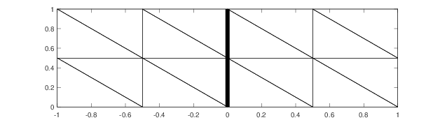
Figure 1: Regular triangular meshes: $4\times 2$ mesh (Left) and $8\times 4$ mesh (Right)

Tables 1 and 2 show the history of convergence for the velocity $\bm{u}_{h0}$, pressure $p_{h0}$, and temperature $T_{h0}$. Results of $div_{h}U_{h}=:\max\limits_{K\in\mathcal{T}_{h}^{f}}h_{K}^{-1}\lVert\nabla\cdot\bm{u}_{h0}\rVert_{0,K}$ are also listed. From the numerical results we have the following observations:

• The convergence rates of $\lVert\nabla\bm{u}-\nabla_{h}\bm{u}_{h0}\rVert_{0},$ $\lVert p-p_{h0}\rVert_{0}$, and $\lVert\nabla T-\nabla_{h}T_{h0}\rVert_{0}$ for the proposed WG methods with $k=1,2$ are of $k^{\text{th}}$ orders, as is consistent with the theoretical results. In addition, the convergence rates of $\lVert\bm{u}-\bm{u}_{h0}\rVert_{0}$ and $\lVert T-T_{h0}\rVert_{0}$ are of $(k+1)^{\text{th}}$ orders.

• Since $\lVert\nabla_{h}\cdot\bm{u}_{h0}\rVert_{0,\infty}\apprle\max\limits_{K\in\mathcal{T}_{h}^{f}}h_{K}^{-1}\lVert\nabla\cdot\bm{u}_{h0}\rVert_{0,K}$, the velocity approximations obtained by our methods are globally divergence-free, which are conformable to the conclusion in Remark 2.1.

Table 1: Results for different methods with $k=1$

mesh	$\frac{\lVert\nabla\bm{u}-\nabla_{h}\bm{u}_{h0}\rVert_{0}}{\lVert\nabla\bm{u}\rVert_{0}}$		$\frac{\lVert\bm{u}-\bm{u}_{h0}\rVert_{0}}{\lVert\bm{u}\rVert_{0}}$		$\frac{\lVert p-p_{h0}\rVert_{0}}{\lVert p\rVert_{0}}$		$\frac{\lVert\nabla T-\nabla_{h}T_{h0}\rVert_{0}}{\lVert\nabla T\rVert_{0}}$		$\frac{\lVert T-T_{h0}\rVert_{0}}{\lVert T\rVert_{0}}$		$div_{h}U_{h}$
	error	order	error	order	error	order	error	order	error	order
$8\times 4$	5.9412E-01		1.6959E-01		4.4819E-01		2.4656E-01		2.7341E-02		3.9988E-16
$16\times 8$	3.1494E-01	0.92	4.7778E-02	1.83	2.3637E-01	0.92	1.2464E-01	0.98	6.8747E-03	1.99	1.9062E-15
$32\times 16$	1.5988E-01	0.98	1.2396E-02	1.95	1.1983E-01	0.98	6.2498E-02	0.99	1.7191E-03	2.00	3.0715E-15
$64\times 32$	8.0247E-02	0.99	3.1249E-03	1.99	6.0122E-02	0.99	3.1272E-02	1.00	4.2894E-04	2.00	3.1834E-14
$128\times 64$	4.0162E-02	1.00	7.8018E-04	2.00	3.0087E-02	1.00	1.5639E-02	1.00	1.0704E-04	2.00	4.6475E-14

(a) Method:WG-I

mesh	$\frac{\lVert\nabla\bm{u}-\nabla_{h}\bm{u}_{h0}\rVert_{0}}{\lVert\nabla\bm{u}\rVert_{0}}$		$\frac{\lVert\bm{u}-\bm{u}_{h0}\rVert_{0}}{\lVert\bm{u}\rVert_{0}}$		$\frac{\lVert p-p_{h0}\rVert_{0}}{\lVert p\rVert_{0}}$		$\frac{\lVert\nabla T-\nabla_{h}T_{h0}\rVert_{0}}{\lVert\nabla T\rVert_{0}}$		$\frac{\lVert T-T_{h0}\rVert_{0}}{\lVert T\rVert_{0}}$		$div_{h}U_{h}$
	error	order	error	order	error	order	error	order	error	order
$8\times 4$	7.0486E-01		7.8104E-01		4.7353E-01		2.6104E-01		1.3922E-01		1.5492E-15
$16\times 8$	3.2996E-01	1.10	1.8899E-01	2.05	2.3962E-01	0.98	1.2868E-01	1.02	3.5017E-02	1.99	5.5321E-16
$32\times 16$	1.6192E-01	1.03	4.8031E-02	1.98	1.2025E-01	0.99	6.4066E-02	1.01	8.7749E-03	2.00	6.8348E-15
$64\times 32$	8.0518E-02	1.01	1.2196E-02	1.98	6.0178E-02	1.00	3.1996E-02	1.00	2.1989E-03	2.00	9.5579E-15
$128\times 64$	4.0158E-02	1.00	3.0774E-03	1.99	3.0095E-02	1.00	1.5993E-02	1.00	5.5203E-04	2.00	2.0390E-14

(b) Method:WG-II

mesh	$\frac{\lVert\nabla\bm{u}-\nabla_{h}\bm{u}_{h0}\rVert_{0}}{\lVert\nabla\bm{u}\rVert_{0}}$		$\frac{\lVert\bm{u}-\bm{u}_{h0}\rVert_{0}}{\lVert\bm{u}\rVert_{0}}$		$\frac{\lVert p-p_{h0}\rVert_{0}}{\lVert p\rVert_{0}}$		$\frac{\lVert\nabla T-\nabla_{h}T_{h0}\rVert_{0}}{\lVert\nabla T\rVert_{0}}$		$\frac{\lVert T-T_{h0}\rVert_{0}}{\lVert T\rVert_{0}}$		$div_{h}U_{h}$
	error	order	error	order	error	order	error	order	error	order
$8\times 4$	7.4774E-01		8.3792E-01		4.7910E-01		3.1663E-01		1.6162E-01		1.0304E-16
$16\times 8$	3.3583E-01	1.02	1.9985E-01	2.07	2.4031E-01	0.99	1.5503E-01	1.03	4.0626E-02	1.99	2.0466E-16
$32\times 16$	1.6272E-01	1.01	5.0551E-02	1.98	1.2033E-01	1.00	7.7080E-02	1.01	1.0178E-02	2.00	1.7369E-15
$64\times 32$	8.0623E-02	1.00	1.2810E-02	1.98	6.0183E-02	1.00	3.8485E-02	1.00	2.5494E-03	2.00	2.3551E-15
$128\times 64$	4.0212E-02	1.00	3.2282E-03	1.99	3.0093E-02	1.00	1.9235E-02	1.00	6.3946E-04	2.00	6.5944E-15

(c) Method:WG-III

Table 2: Results for different methods with $k=2$

mesh	$\frac{\lVert\nabla\bm{u}-\nabla_{h}\bm{u}_{h0}\rVert_{0}}{\lVert\nabla\bm{u}\rVert_{0}}$		$\frac{\lVert\bm{u}-\bm{u}_{h0}\rVert_{0}}{\lVert\bm{u}\rVert_{0}}$		$\frac{\lVert p-p_{h0}\rVert_{0}}{\lVert p\rVert_{0}}$		$\frac{\lVert\nabla T-\nabla_{h}T_{h0}\rVert_{0}}{\lVert\nabla T\rVert_{0}}$		$\frac{\lVert T-T_{h0}\rVert_{0}}{\lVert T\rVert_{0}}$		$div_{h}U_{h}$
	error	order	error	order	error	order	error	order	error	order
$8\times 4$	1.6192E-01		2.8177E-02		6.6611E-02		2.3814E-02		1.5210E-03		1.5852E-15
$16\times 8$	4.2800E-02	1.92	3.6801E-03	2.94	1.7476E-02	1.92	5.9899E-03	1.98	1.9029E-04	2.99	1.3501E-14
$32\times 16$	1.0767E-02	1.99	4.6124E-04	2.99	4.4430E-03	1.98	1.4995E-03	1.99	2.3790E-05	3.00	6.8867E-14
$64\times 32$	2.6808E-03	2.01	5.7386E-05	3.01	1.1115E-03	1.99	3.7495E-04	2.00	2.9736E-06	3.00	3.8064E-14
$128\times 64$	6.7021E-04	2.00	7.1513E-06	3.00	2.7795E-04	2.00	9.3738E-05	2.00	3.7173E-07	3.00	7.2047E-14

(a) Method:WG-I

mesh	$\frac{\lVert\nabla\bm{u}-\nabla_{h}\bm{u}_{h0}\rVert_{0}}{\lVert\nabla\bm{u}\rVert_{0}}$		$\frac{\lVert\bm{u}-\bm{u}_{h0}\rVert_{0}}{\lVert\bm{u}\rVert_{0}}$		$\frac{\lVert p-p_{h0}\rVert_{0}}{\lVert p\rVert_{0}}$		$\frac{\lVert\nabla T-\nabla_{h}T_{h0}\rVert_{0}}{\lVert\nabla T\rVert_{0}}$		$\frac{\lVert T-T_{h0}\rVert_{0}}{\lVert T\rVert_{0}}$		$div_{h}U_{h}$
	error	order	error	order	error	order	error	order	error	order
$8\times 4$	2.5023E-01		5.9209E-02		6.6212E-02		4.1197E-02		4.9610E-03		6.5550E-16
$16\times 8$	6.3163E-02	1.98	7.4474E-03	2.99	1.7485E-02	1.92	1.0276E-02	1.99	6.1111E-04	3.02	7.4872E-15
$32\times 16$	1.5659E-02	2.01	9.3395E-04	2.99	4.4432E-03	1.98	2.5691E-03	2.00	7.5883E-05	3.01	5.6488E-15
$64\times 32$	3.8820E-03	2.01	1.1720E-04	3.00	1.1117E-03	2.00	6.4257E-04	2.00	9.4569E-06	3.00	2.4648E-14
$128\times 64$	9.6547E-04	2.00	1.4685E-05	3.00	2.7815E-04	2.00	1.6070E-04	2.00	1.1804E-06	3.00	2.1412E-13

(b) Method:WG-II

mesh	$\frac{\lVert\nabla\bm{u}-\nabla_{h}\bm{u}_{h0}\rVert_{0}}{\lVert\nabla\bm{u}\rVert_{0}}$		$\frac{\lVert\bm{u}-\bm{u}_{h0}\rVert_{0}}{\lVert\bm{u}\rVert_{0}}$		$\frac{\lVert p-p_{h0}\rVert_{0}}{\lVert p\rVert_{0}}$		$\frac{\lVert\nabla T-\nabla_{h}T_{h0}\rVert_{0}}{\lVert\nabla T\rVert_{0}}$		$\frac{\lVert T-T_{h0}\rVert_{0}}{\lVert T\rVert_{0}}$		$div_{h}U_{h}$
	error	order	error	order	error	order	error	order	error	order
$8\times 4$	1.3075E-01		6.2217E-02		6.6237E-02		2.1605E-02		5.3332E-03		1.6739E-15
$16\times 8$	3.4979E-02	1.90	7.6750E-03	3.02	1.7492E-02	1.92	5.4667E-03	1.98	6.6033E-04	3.02	3.5685E-15
$32\times 16$	8.9627E-03	1.96	9.4948E-04	3.01	4.4333E-03	1.98	1.3734E-03	1.99	8.2232E-05	3.01	3.2603E-14
$64\times 32$	2.2617E-03	1.99	1.1834E-04	3.00	1.1121E-03	2.00	3.4409E-04	2.00	1.0263E-05	3.00	7.3185E-14
$128\times 64$	5.6761E-04	2.00	1.4791E-05	3.00	2.7826E-04	2.00	8.6112E-05	2.00	1.2821E-06	3.00	2.6642E-13

(c) Method:WG-III

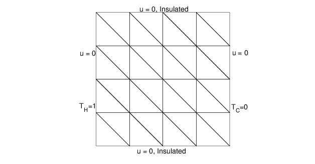
Figure 2: The physical domain with its boundary conditions: $4\times 4$ mesh

Example 6.2.

We consider the well-known test cave for the natural convection codes which is called buoyancy-driven cavity problem. This problem describes the two-dimensional flow of a Boussinesq fluid in an upright square cavity of side $L=1$. Fig.2 shows the physical domain with the boundary conditions. The velocity is zero on all the boundaries. The horizontal walls are insulated with $\frac{\partial T}{\partial\bm{n}}=0$, and the vertical sides are at temperatures $T_{H}=1$ and $T_{C}=0$. We take $\Omega=\Omega_{f}=[0,1]\times[0,1]$, $\kappa=1,\Pr=0.71,\bm{f}=0$, and $g=0$.

For different Rayleigh numbers, i.e. $Ra=10^{3},10^{4},10^{5},10^{6},10^{7}$, we use the WG-I method with $k=1,2$ to compute the following quantities at different mesh sizes:

$u1_{max}$	the maximum horizontal velocity on the vertical mid-plane of the cavity
$u2_{max}$	the maximum vertical velocity on the horizontal mid-plane of the cavity
$\overline{Nu}$	the average Nusselt number throughout the cavity
$Nu_{max}$	the maximum value of the local Nusselt number on the boundary at x=0
$Nu_{min}$	the minimum value of the local Nusselt number on the boundary at x=0

The results are listed in Table 3 and compared with the famous benchmark solutions of de Vahl Davis [12] and of some other authors such as Manzari [21], Massarotti et al [22], Wan et al [29], and Zhang et al [38]. Figure 3 and Figure 4 show the contour maps of the stream function and the isotherms of the flow. We have the following observations:

• From Table 3 we can see that the WG-I method gives good results for all the quantities for different Rayleigh numbers. In particular, the method with $k=2$ behaves very well at the coarsest mesh $40\times 40$.

• Figure 3 demonstrates that, as Rayleigh number $Ra$ increases, the circular vortex at the cavity center begins to deform into an ellipse and then breaks up into two vortices, and then there’s a big vortex in the center.

• Figure 4 shows that, when Rayleigh number $Ra$ is small, the heat transfer mainly depends on heat conduction (isotherms almost vertical), with the increasing of $Ra$, the heat transfer pattern gradually turns to heat convection and boundary layers appear around the two walls (isotherms almost horizontal at the center).

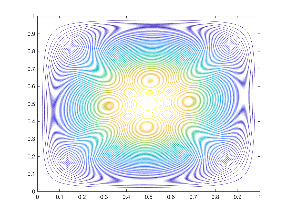
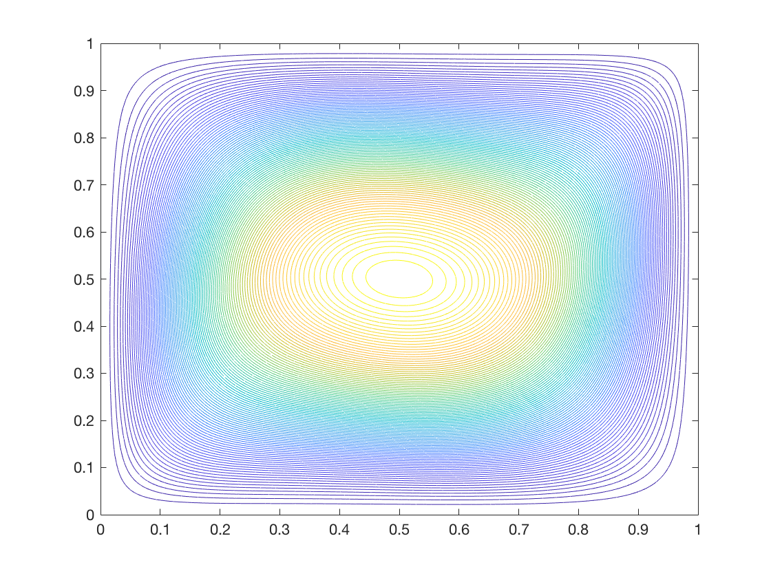
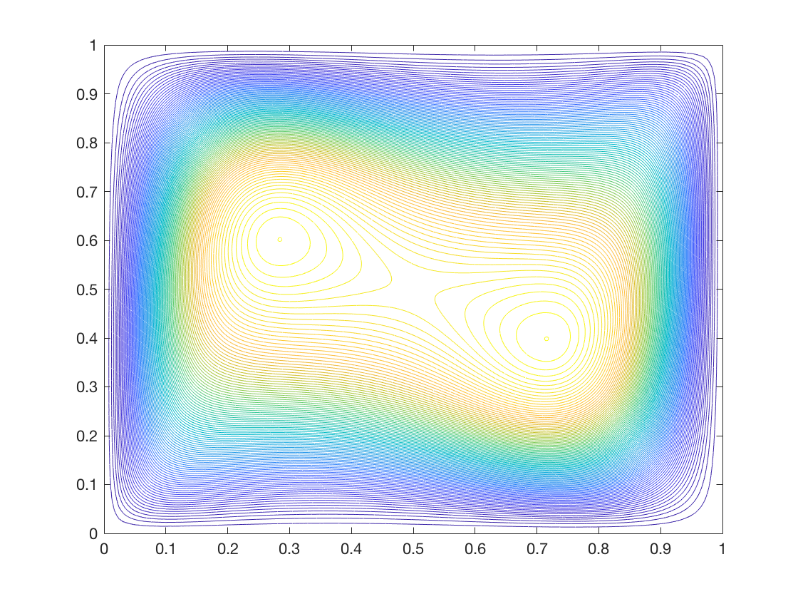
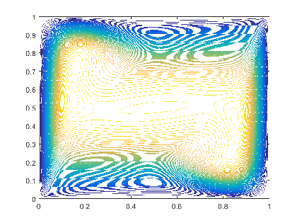
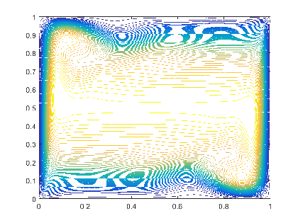
Figure 3: Contour maps of stream function (left to right) with Ra = $10^{3},10^{4},10^{5},10^{6},10^{7}$.

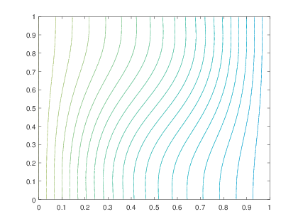
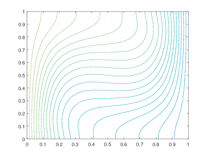
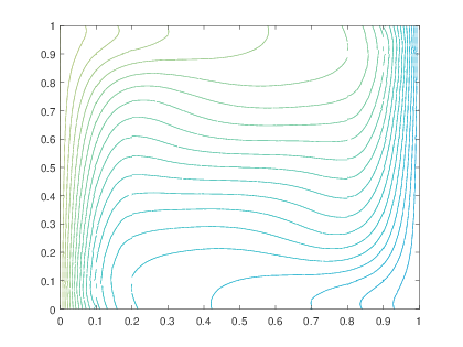
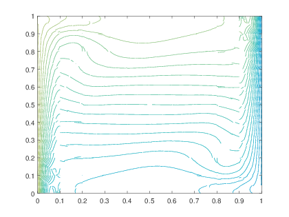
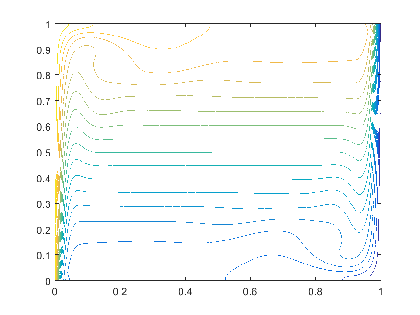
Figure 4: Isotherms(left to right) with Ra = $10^{3},10^{4},10^{5},10^{6},10^{7}$

Table 3: Natural convection in a square cavity: comparison with the benchmark solutions

Ra		WG-I,k=1	WG-I,k=1	WG-I,k=2	WG-I,k=2	Ref.[12]	Ref.[38]	Ref.[21]	Ref.[22]	Ref.[29]
		$40\times 40$	$70\times 70$	$40\times 40$	$50\times 50$		$64\times 64$	$70\times 70$	$70\times 70$	$100\times 100$
$10^{3}$	$u1_{max}$	3.653	3.654	3.640	3.646	3.649	-	3.68	-	3.489
	$u2_{max}$	3.711	3.698	3.697	3.697	3.697	-	3.73	3.686	3.69
	$\overline{Nu}$	1.118	1.118	1.118	1.118	1.118	-	1.074	1.117	1.117
	$Nu_{max}$	1.506	1.506	1.560	1.506	1.505	-	1.47	-	1.501
	$Nu_{min}$	0.691	0.691	0.691	0.691	0.692	-	0.623	-	0.691
$10^{4}$	$u1_{max}$	16.227	16.188	16.183	16.180	16.178	16.19	16.10	-	16.122
	$u2_{max}$	19.744	19.611	19.600	16.628	19.617	19.63	19.90	19.63	19.79
	$\overline{Nu}$	2.243	2.244	2.245	2.245	2.243	-	2.084	2.243	2.254
	$Nu_{max}$	3.528	3.530	3.531	3.531	3.528	-	3.47	-	3.579
	$Nu_{min}$	0.585	0.585	0.585	0.585	0.586	-	0.4968	-	0.577
$10^{5}$	$u1_{max}$	34.829	34.771	34.715	34.702	34.81	34.74	34.00	-	34.00
	$u2_{max}$	69.049	68.736	67.875	68.290	68.22	68.48	70.00	68.85	70.63
	$\overline{Nu}$	4.515	4.519	4.522	4.522	4.519	-	4.30	4.521	4.598
	$Nu_{max}$	7.701	7.713	7.716	7.720	7.717	-	7.71	-	7.945
	$Nu_{min}$	0.726	0.727	0.728	0.728	0.729	-	0.614	-	0.698
$10^{6}$	$u1_{max}$	64.977	64.710	64.835	64.541	64.63	64.81	65.40	-	65.40
	$u2_{max}$	217.307	221.534	208.237	220.609	219.36	220.46	228	221.6	227.11
	$\overline{Nu}$	8.797	8.813	8.825	8.825	8.800	-	8.743	8.806	8.976
	$Nu_{max}$	17.676	17.511	17.462	17.536	17.925	-	17.46	-	17.86
	$Nu_{min}$	0.970	0.976	0.980	0.979	0.989	-	0.716	-	0.913
$10^{7}$	$u1_{max}$	154.770	148.802	148.454	148.596	145.267*	148.40	139.7	-	143.56
	$u2_{max}$	819.329	695.512	703.702	707.696	703.253*	694.14	698	702.3	714.48
	$\overline{Nu}$	16.564	16.484	16.522	16.521	-	-	13.99	16.40	16.656
	$Nu_{max}$	47.155	40.374	40.935	40.329	41.025*	-	30.46	-	38.6
	$Nu_{min}$	1.359	1.353	1.363	1.367	1.380*	-	0.787	-	1.298

• The benchmark solutions with * were mentioned in [23] when $Ra=10^{7}$.

7 Conclusions

In this paper, we have developed a class of weak Galerkin finite element methods with globally divergence-free velocity approximation for the steady-state natural convection problems. Well-posedness of the discrete scheme is analyzed, and optimal error estimates for the velocity, temperature and pressure approximations are derived. The proposed Oseen’s iteration algorithm is unconditionally convergent. Numerical experiments verify the theoretical results.

References

- [1] M. Benítez and A. Bermúdez. A second order characteristics finite element scheme for natural convection problems. Journal of Computational and Applied Mathematics, 235(11):3270–3284, 2011.
- [2] J. Boland and W. Layton. An analysis of the finite element method for natural convection problems. Numerical Methods for Partial Differential Equations, 6(2):115–126, 1990.
- [3] J. Boland and W. Layton. Error analysis for finite element methods for steady natural convection problems. Numerical functional analysis and optimization, 11(5-6):449–483, 1990.
- [4] H. Brezis. Functional analysis, Sobolev spaces and partial differential equations. Springer Science & Business Media, 2010.
- [5] F. Brezzi, D. Boffi, L. Demkowicz, R.G. Durán, R.S. Falk, and M. Fortin. Mixed finite elements, compatibility conditions, and applications. Springer, 2008.
- [6] G. Chen, M. Feng, and X. Xie. Robust globally divergence-free weak Galerkin methods for Stokes equations. Journal of Computational Mathematics, 34(5):549–572, 2016.
- [7] G. Chen, M. Feng, and X. Xie. A robust WG finite element method for convection–diffusion–reaction equations. Journal of Computational and Applied Mathematics, 315:107–125, 2017.
- [8] G. Chen and X. Xie. A robust weak Galerkin finite element method for linear elasticity with strong symmetric stresses. Computational Methods in Applied Mathematics, 16(3):389–408, 2016.
- [9] L. Chen, J. Wang, Y. Wang, and X. Ye. An auxiliary space multigrid preconditioner for the weak Galerkin method. Computers & Mathematics with Applications, 70(4):330–344, 2015.
- [10] Y. Chen, G. Chen, and X. Xie. Weak Galerkin finite element method for Biot’s consolidation problem. Journal of Computational and Applied Mathematics, 330:398–416, 2018.
- [11] B. Cockburn, J. Gopalakrishnan, and R. Lazarov. Unified hybridization of discontinuous Galerkin, mixed, and continuous galerkin methods for second order elliptic problems. Siam Journal on Numerical Analysis, 47(2):1319–1365, 2009.
- [12] G. de Vahl Davis. Natural convection of air in a square cavity: a bench mark numerical solution. International Journal for numerical methods in fluids, 3(3):249–264, 1983.
- [13] B. Deka. A weak galerkin finite element method for elliptic interface problems with polynomial reduction. Numerical Mathematics-Theory Methods and Applications, 11:655–672, 2018.
- [14] O.A. Karakashian and F. Pascal. Convergence of adaptive discontinuous galerkin approximations of second-order elliptic problems. SIAM Journal on Numerical Analysis, 45(2):641–665, 2007.
- [15] H.W.J. Lenferink. An accurate solution procedure for fluid flow with natural convection. Numerical Functional Analysis and Optimization, 15(5-6):661–687, 1994.
- [16] B. Li and X. Xie. A two-level algorithm for the weak Galerkin discretization of diffusion problems. Journal of Computational and Applied Mathematics, 287:179–195, 2015.
- [17] B. Li and X. Xie. BPX preconditioner for nonstandard finite element methods for diffusion problems. SIAM Journal on Numerical Analysis, 54(2):1147–1168, 2016.
- [18] J. Loewe and G. Lube. A projection-based variational multiscale method for large-eddy simulation with application to non-isothermal free convection problems. Mathematical Models and Methods in Applied Sciences, 22(02):1150011, 2012.
- [19] Z. Luo, J. Chen, I.M. Navon, and J. Zhu. An optimizing reduced plsmfe formulation for non-stationary conduction–convection problems. International Journal for Numerical Methods in Fluids, 60(4):409–436, 2009.
- [20] Z. Luo and X. Lu. A least squares galerkin/petrov mixed finite element method for the stationary conduction-convection problems. MATHEMATICA NUMERICA SINICA-CHINESE EDITION, 25(2):231–244, 2003.
- [21] M.T. Manzari. An explicit finite element algorithm for convection heat transfer problems. International Journal of Numerical Methods for Heat & Fluid Flow, 9(8):860–877, 1999.
- [22] N. Massarotti, P. Nithiarasu, and O.C. Zienkiewicz. Characteristic-based-split (cbs) algorithm for incompressible flow problems with heat transfer. International Journal of Numerical Methods for Heat & Fluid Flow, 8(8):969–990, 1998.
- [23] D.A. Mayne, A.S. Usmani, and M. Crapper. h-adaptive finite element solution of high rayleigh number thermally driven cavity problem. International Journal of Numerical Methods for Heat & Fluid Flow, 10(6):598–615, 2000.
- [24] L. Mu, J. Wang, X. Ye, and S. Zhang. A weak Galerkin finite element method for the Maxwell equations. Journal of Scientific Computing, 65(1):363–386, 2015.
- [25] D. Shi and J. Ren. Nonconforming mixed finite element method for the stationary conduction-convection problem. International Journal of Numerical Analysis & Modeling, 6(2), 2009.
- [26] D. Shi and J. Ren. A least squares galerkin–petrov nonconforming mixed finite element method for the stationary conduction–convection problem. Nonlinear Analysis Theory Methods and Applications, 72(3–4):1653–1667, 2010.
- [27] Z. Shi and M. Wang. Finite element methods. Science Press, 2013.
- [28] Z. Si and Y. He. A defect-correction mixed finite element method for stationary conduction-convection problems. Mathematical Problems in Engineering, 2011, 2011.
- [29] C. Wan, B.S.V. Patnaik, and G.W. Wei. A new benchmark quality solution for the buoyancy-driven cavity by discrete singular convolution. Numerical Heat Transfer: Part B: Fundamentals, 40(3):199–228, 2001.
- [30] J. Wang and X. Ye. A weak Galerkin finite element method for second-order elliptic problems. Journal of Computational and Applied Mathematics, 241:103–115, 2013.
- [31] J. Wang and X. Ye. A weak Galerkin mixed finite element method for second order elliptic problems. Mathematics of Computation, 83(289):2101–2126, 2014.
- [32] J. Wang and X. Ye. A weak Galerkin finite element method for the Stokes equations. Advances in Computational Mathematics, 42(1):155–174, 2016.
- [33] R. Wang, X. Wang, Q. Zhai, and R. Zhang. A weak Galerkin finite element scheme for solving the stationary Stokes equations. Journal of Computational and Applied Mathematics, 302:171–185, 2016.
- [34] R. Wang, X. Wang, and R. Zhang. A weak galerkin finite element method for elliptic interface problems with polynomial reduction. Numerical Mathematics-Theory Methods and Applications, 11:518–539, 2018.
- [35] Q. Zhai, R. Zhang, N. Malluwawadu, and S. Hussain. The weak Galerkin method for linear hyperbolic equation. Communications in Computational Physics, 24:152–166, 2018.
- [36] J. Zhang, K. Zhang, J. Li, and X. Wang. A weak Galerkin finite element method for the Navier-Stokes equations. Communications in Computational Physics, 23:706–746, 2018.
- [37] T. Zhang, X. Zhao, and P. Huang. Decoupled two level finite element methods for the steady natural convection problem. Numerical Algorithms, 68(4):837–866, 2015.
- [38] Y. Zhang, Y. Hou, and J. Zhao. Error analysis of a fully discrete finite element variational multiscale method for the natural convection problem. Computers & Mathematics with Applications, 68(4):543–567, 2014.
- [39] Y. Zhang, Y. Hou, and H. Zheng. A finite element variational multiscale method for steady-state natural convection problem based on two local gauss integrations. Numerical methods for partial differential equations, 30(2):361–375, 2014.
- [40] X. Zheng, G. Chen, and X. Xie. A divergence-free weak Galerkin method for quasi-Newtonian Stokes flows. Science China Mathematics, 60(8):1515–1528, 2017.
- [41] X. Zheng and X. Xie. A posteriori error estimator for a weak Galerkin finite element solution of the Stokes problem. East Asian Journal on Applied Mathematics, 7(3):508–529, 2017.