Parallel Adaptive Sampling
with almost no Synchronization

Abstract

Approximation via sampling is a widespread technique whenever exact solutions are too expensive. In this paper, we present techniques for an efficient parallelization of adaptive (a. k. a. progressive) sampling algorithms on multi-threaded shared-memory machines. Our basic algorithmic technique requires no synchronization except for atomic load-acquire and store-release operations. It does, however, require $\mathcal{O}(n)$ memory per thread, where $n$ is the size of the sampling state. We present variants of the algorithm that either reduce this memory consumption to $\mathcal{O}(1)$ or ensure that deterministic results are obtained.

Using the KADABRA algorithm for betweenness centrality (a popular measure in network analysis) approximation as a case study, we demonstrate the empirical performance of our techniques. In particular, on a 32-core machine, our best algorithm is $\numprint{2.8809418644086824}\times$ faster than what we could achieve using a straightforward OpenMP-based parallelization and $\numprint{65.29488898389054}\times$ faster than the existing implementation of KADABRA.

1 Introduction

When a computational problem cannot be solved exactly within the desired time budget, a frequent solution is to employ approximation algorithms [12]. With large data sets being the rule and not the exception today, approximation is frequently applied, even to polynomial-time problems [6]. We focus on a particular subclass of approximation algorithms: sampling algorithms. They sample data according to some (usually algorithm-specific) probability distribution, perform some computation on the sample and induce a result for the full data set.

More specifically, we consider adaptive sampling (ADS) algorithms (also called progressive sampling algorithms). Here, the number of samples that are required is not statically computed (e. g., from the input instance) but also depends on the data that has been sampled so far. While non-adaptive sampling algorithms can often be parallelized trivially by drawing multiple samples in parallel, adaptive sampling constitutes a challenge for parallelization: checking the stopping condition of an ADS algorithm requires access to all the data generated so far and thus mandates some form of synchronization.

Motivation and Contribution.

Our initial motivation was a parallel implementation of the sequential state-of-the-art approximation algorithm KADABRA [6] for betweenness centrality (BC) approximation. BC is a very popular centrality measure in network analysis, see Section 2.2 for more details. To the best of our knowledge, parallel adaptive sampling has not received a generic treatment yet. Hence, we propose techniques to parallelize ADS algorithms in a generic way, while scaling to large numbers of threads. While we turn to KADABRA to demonstrate the effectiveness of the proposed algorithms, our techniques can be adjusted easily to other ADS algorithms.

We introduce two new parallel ADS algorithms, which we call local-frame and shared-frame. Both algorithms try to avoid extensive synchronization when checking the stopping condition. This is done by maintaining multiple copies of the sampling state and ensuring that the stopping condition is never checked on a copy of the state that is currently being written to. Local-frame is designed to use the least amount of synchronization possible – at the cost of an additional memory footprint of $\Theta(n)$ per thread, where $n$ denotes the size of the sampling state. This algorithm performs only atomic load-acquire and store-release operations for synchronization, but no expensive read-modify-write operations (like CAS or fetch-add). Shared-frame, in turn, aims instead at meeting a desired tradeoff between memory footprint and synchronization overhead. In contrast to local-frame, it requires only $\Theta(1)$ additional memory per thread, but uses atomic read-modify-write operations (e. g., fetch-add) to accumulate samples. We also propose the deterministic indexed-frame algorithm; it guarantees that the results of two different executions is the same for a fixed random seed, regardless of the number of threads.

Our experimental results show that local-frame, shared-frame and indexed-frame achieve parallel speedups of $\numprint{15.879639123178466}\times$, $\numprint{18.081267115073295}\times$, and $\numprint{10.818961592817336}\times$ on 32 cores, respectively. Using the same number of cores, our OpenMP-based parallelization (functioning as a baseline) only yields a speedup of $\numprint{6.27616521473421}\times$; thus our algorithms are up to $\numprint{2.8809418644086824}\times$ faster. Moreover, also due to implementation improvements and parameter tuning, our best algorithm performs adaptive sampling $\numprint{65.29488898389054}\times$ faster than the existing implementation of KADABRA (when all implementations use 32 cores).

2 Preliminaries and Baseline for Parallelization

2.1 Basic Definitions

Memory model.

Throughout this paper, we target a multi-threaded shared-memory machine with $T$ threads. We work in the C11 memory model [13] (more details in Appendix 0.A); in particular, we assume the existence of the usual atomic operations, as well as load-acquire and store-release barriers.

Adaptive sampling.

Algorithm 1 Generic Adaptive Sampling

Variable initialization:

$d\leftarrow$ new sampling state structure

$d\mathtt{.data}\leftarrow(0,\ldots,0)$ $\triangleright$ Sampled data.

$d\mathtt{.num}\leftarrow 0$ $\triangleright$ Number of samples.

Main loop:

while not checkForStop($d$) do

     $d\mathtt{.data}\leftarrow d\mathtt{.data}\circ\textsc{sample}(\hbox{})$

     $d\mathtt{.num}\leftarrow d\mathtt{.num}+1$

For our techniques to be applicable, we expect that an ADS algorithm behaves as depicted in Algorithm 1: it iteratively samples data (in sample) and aggregates it (using some operator $\circ$), until a stopping condition (checkForStop) determines that the data sampled so far is sufficient to return an approximate solution within the required accuracy. This condition does not only consider the number of samples ($d\mathtt{.num}$), but also the sampled data ($d\mathtt{.data}$). Throughout this paper, we denote the size of that data (i. e., the number of elements of $d.\mathtt{data}$) by $n$. We assume that the stopping condition needs to be checked on a consistent state, i. e., a state of $d$ that can occur in a sequential execution. Furthermore, to make parallelization feasible at all, we need to assume that $\circ$ is associative.

2.2 Betweenness Centrality and its Approximation

Betweenness Centrality (BC) is one of the most popular vertex centrality measures in the field of network analysis. Such measures indicate the importance of a vertex based on its position in the network [4] (we use the terms graph and network interchangeably). Being a centrality measure, BC constitutes a function $\mathbf{b}:V\to\mathbb{R}$ that maps each vertex of a graph $G=(V,E)$ to a real number – higher numbers represent higher importance. To be precise, the BC of $u\in V$ is defined as $\mathbf{b}(u)=\sum_{s\neq t\in V\setminus\{u\}}\frac{\sigma_{st}(u)}{\sigma_{st}},$ where $\sigma_{st}$ is the number of shortest $s$-$t$-paths and $\sigma_{st}(u)$ is the number of shortest $s$-$t$-paths that contain $u$.

Unfortunately, BC is rather expensive to compute: the standard exact algorithm [8] has time complexity $\Theta(|V||E|)$ for unweighted graphs. Moreover, unless the Strong Exponential Time Hypothesis fails, this asymptotic running time cannot be improved [5]. Numerous approximation algorithms for BC have thus been developed (we refer to Section 5 for an overview). The state of the art of these approximation algorithms is the KADABRA algorithm [6] of Borassi and Natale, which happens to be an ADS algorithm. With probability $(1-\delta)$, KADABRA approximates the BC values of the vertices within an additive error of $\epsilon$ in nearly-linear time complexity, where $\epsilon$ and $\delta$ are user-specified constants.

While our techniques apply to any ADS algorithm, we recall that, as a case study, we focus on scaling the KADABRA algorithm to a large number of threads.

2.3 The KADABRA algorithm

KADABRA samples vertex pairs $(s,t)$ of $G=(V,E)$ uniformly at random and then selects a shortest $s$-$t$-path uniformly at random (in sample in Algorithm 1). After $\tau$ iterations, this results in a sequence of randomly selected shortest paths $\pi_{1},\pi_{2},\dots,\pi_{\tau}$; from those paths, BC is estimated as:

$$\widetilde{\mathbf{b}}(v)=\frac{1}{\tau}\sum_{i=1}^{\tau}x_{i}(v),\quad x_{i}(v)=\begin{cases}1&\text{ if }v\in\pi_{i}\\ 0&\text{otherwise.}\end{cases}$$

$\sum_{i=1}^{\tau}x_{i}$ is exactly the sampled data ($d\mathtt{.data}$) that the algorithm has to store (i. e., the accumulation $\circ$ in Algorithm 1 sums $x_{i}$ over $i$). To compute the stopping condition (checkForStop in Algorithm 1), KADABRA maintains the invariants

$$\Pr(\mathbf{b}(v)\leq\widetilde{\mathbf{b}}(v)-f)\leq\delta_{L}(v)\text{ ~{}and~{} }\Pr(\mathbf{b}(v)\geq\widetilde{\mathbf{b}}(v)+g)\leq\delta_{U}(v)$$ (1)

for two functions $f=f(\widetilde{\mathbf{b}}(v),\delta_{L}(v),\omega,\tau)$ and $g=g(\widetilde{\mathbf{b}}(v),\delta_{U}(v),\omega,\tau)$ depending on a maximal number $\omega$ of samples and per-vertex probability constants $\delta_{L}$ and $\delta_{U}$ (more details in the original paper [6]). The values of those constants are computed in a preprocessing phase (mostly consisting of computing an upper bound on the diameter of the graph). $\delta_{L}$ and $\delta_{U}$ satisfy $\sum_{v\in V}\delta_{L}(v)+\delta_{U}(v)\leq\delta$ for a user-specified parameter $\delta\in(0,1)$. Thus, the algorithm terminates once $f,g<\epsilon$; the result is correct with an absolute error of $\pm\epsilon$ and probability $(1-\delta)$. We note that checking the stopping condition of KADABRA on an inconsistent state leads to incorrect results. For example, this can be seen from the fact that $g$ is increasing with $\widetilde{\mathbf{b}}$ and decreasing with $\tau$, see Appendix 0.B.

2.4 First Attempts at KADABRA Parallelization

In the original KADABRA implementation, a lock is used to synchronize concurrent access to the sampling state. As a first attempt to improve the scalability, we consider an algorithm that iteratively computes a fixed number of samples in parallel (e. g., using an OpenMP parallel for loop), then issues a synchronization barrier (as implied by the parallel for loop) and checks the stopping condition afterwards. While sampling, atomic increments are used to update the global sampling data. This algorithm is arguably the “natural” OpenMP-based parallelization of an ADS algorithm and can be implemented in a few extra lines of code. Moreover, it already improves upon the original parallelization. However, as shown by the experiments in Section 4, further significant improvements in performance are possible by switching to more lightweight synchronization.

3 Scalable Parallelization Techniques

To improve upon the OpenMP parallelization from Section 2.4, we have to avoid the synchronization barrier before the stopping condition can be checked. This is the objective of our epoch-based algorithms that constitute the main contribution of this paper. In Section 3.1, we formulate the main idea of our algorithms as a general framework and prove its correctness. The subsequent subsections present specific algorithms based on this framework and discuss tradeoffs between them.

3.1 Epoch-based Framework

int epoch $\leftarrow e$ int num $\leftarrow 0$ int data[$n$] $\leftarrow(0,\ldots,0)$

(a) Structure of a state frame (SF) for epoch $e$. num: Number of samples, data: Sampled data

bool	stop	$\leftarrow$ false
int	epochToRead	$\leftarrow 0$
SF $\ast$	sfFin[$T$]	$\leftarrow(\textsf{null},\ldots,\textsf{null})$

(b) Shared variables

Figure 1: Data structures used in epoch-based algorithms, including initial values

In our epoch-based algorithms, the execution of each thread is subdivided into a sequence of discrete epochs. During an epoch, each thread iteratively collects samples; the stopping condition is only checked at the end of an epoch. The crucial advantage of this approach is that the end of an epoch does not require global synchronization. Instead, our framework guarantees the consistency of the sampled data by maintaining multiple copies of the sampling state.

As an invariant, it is guaranteed that that no thread writes to a copy of the state that is currently being read by another thread. This is achieved as follows: each copy of the sampling state is labeled by an epoch number $e$, i. e., a monotonically increasing integer that identifies the epoch in which the data was generated. When the stopping condition has to be checked, all threads advance to a new epoch $e+1$ and start writing to a new copy of the sampling state. The stopping condition is only verified after all threads have finished this transition and it only takes the sampling state of epoch $e$ into account.

More precisely, the main data structure that we use to store the sampling state is called a state frame (SF). Each SF $f$ (depicted in Figure 1(a)) consists of (i) an epoch number ($f.\mathtt{epoch}$), (ii) a number of samples ($f.\mathtt{num}$) and (iii) the sampled data ($f.\mathtt{data}$). The latter two symbols directly correspond to $d.\texttt{num}$ and $d.\mathtt{data}$ in our generic formulation of an adaptive sampling algorithm (Algorithm 1). Aside from the SF structures, our framework maintains three global variables that are shared among all threads (depicted in Figure 1(b)): (i) a simple Boolean flag stop to determine if the algorithm should terminate, (ii) a variable epochToRead that stores the number of the epoch that we want to check the stopping condition on and (iii) a pointer sfFin[$t$] for each thread $t$ that points to a SF finished by thread $t$. Incrementing $\mathtt{epochToRead}$ is our synchronization mechanism to notify all threads that they should advance to a new epoch. This transition is visualized in Figure 4 in Appendix 0.D.1.

Algorithm 2 Epoch-based Approach

Per-thread variable initialization:

$e_{\mathrm{sam}}\leftarrow 1$

$f_{\mathrm{sam}}\leftarrow$ new SF for $e_{\mathrm{sam}}=1$

if $t=0$ then

     $e_{\mathrm{chk}}\leftarrow 0$

     $inCheck\leftarrow$ false

Main loop for thread $t$:

1:loop

2:     $doStop\operatorname{\leftarrow_{\mathsf{relaxed}}}\mathtt{stop}$

3:     if $doStop$ then

4:         break      

5:     $f_{\mathrm{sam}}\mathtt{.data}\leftarrow f_{\mathrm{sam}}\mathtt{.data}\circ\textsc{sample}(\hbox{})$

6:     $f_{\mathrm{sam}}\mathtt{.num}\leftarrow f_{\mathrm{sam}}\mathtt{.num}+1$

7:     $r\operatorname{\leftarrow_{\mathsf{relaxed}}}$ epochToRead

8:     if $r=$ $e_{\mathrm{sam}}$ then

9:         reclaim SF of epoch $e_{\mathrm{sam}}-1$

10:         sfFin[t] $\operatorname{\leftarrow_{\mathsf{release}}}$ $f_{\mathrm{sam}}$

11:         $e_{\mathrm{sam}}$ $\leftarrow$ $e_{\mathrm{sam}}$ $+1$

12:         $f_{\mathrm{sam}}$ $\leftarrow$ new SF for $e_{\mathrm{sam}}$      

13:     if $t=0$ then

14:         checkFrames()      

Check of stopping condition by thread $0$:

15:procedure checkFrames()

16:     if not $inCheck$ then

17:         $e_{\mathrm{chk}}\leftarrow e_{\mathrm{chk}}+1$

18:         epochToRead $\operatorname{\leftarrow_{\mathsf{relaxed}}}e_{\mathrm{chk}}$

19:         $inCheck\leftarrow$ true      

20:     for $i\in\{1,\ldots,T\}$ do

21:         $f_{\mathrm{fin}}\operatorname{\leftarrow_{\mathsf{acquire}}}$ sfFin[t]

22:         if $f_{\mathrm{fin}}=\mathsf{null}$ then

23:              return          

24:         if $f_{\mathrm{fin}}$.epoch $\neq e_{\mathrm{chk}}$ then

25:              return               

26:     $d\leftarrow$ new SF for accumulation

27:     for $i\in\{1,\ldots,T\}$ do

28:         $f_{\mathrm{fin}}\operatorname{\leftarrow_{\mathsf{relaxed}}}$ sfFin[t]

29:         $d\mathtt{.data}\leftarrow d\mathtt{.data}\circ f_{\mathrm{fin}}\mathtt{.data}$

30:         $d\mathtt{.num}\leftarrow d\mathtt{.num}+f_{\mathrm{fin}}\mathtt{.num}$      

31:     if checkForStop($d$) then

32:         $\mathtt{stop}\operatorname{\leftarrow_{\mathsf{relaxed}}}$ true      

33:     $inCheck\leftarrow$ false

Algorithm 2 states the pseudocode of our framework. By $\operatorname{\leftarrow_{\mathsf{relaxed}}}$, $\operatorname{\leftarrow_{\mathsf{acquire}}}$ and $\operatorname{\leftarrow_{\mathsf{release}}}$, we denote relaxed memory access, load-acquire and store-release, respectively (see Sections 2.1 and Appendix 0.A). In the algorithm, each thread maintains an epoch number $e_{\mathrm{sam}}$. To be able to check the stopping condition, thread 0 maintains another epoch number $e_{\mathrm{chk}}$. Indeed, thread 0 is the only thread that evaluates the stopping condition (in checkFrames) after accumulating the SFs from all threads. checkFrames determines whether there is an ongoing check for the stopping condition ($inCheck$ is true; line 16). If that is not the case, a check is initiated (by incrementing $e_{\mathrm{chk}}$) and all threads are signaled to advance to the next epoch (by updating epochToRead). Afterwards, checkFrames only continues if all threads $t$ have published their SFs for checking (i. e., $\mathtt{sfFin}[t]$ points to a SF of epoch $e_{\mathrm{chk}}$; line 20). Once that happens, those SFs are accumulated (line 27) and the stopping condition is checked on the accumulated data (line 31). Eventually, the termination flag (stop; line 32) signals to all threads that they should stop sampling. The main algorithm, on the other hand, performs a loops until this flag is set (line 2). Each iteration collects one sample and writes the results to the current SF ($f_{\mathrm{sam}}$). If a thread needs to advance to a new epoch (because an incremented epochToRead is read in line 7), it publishes its current SF to sfFin and starts writing to a new SF ($f_{\mathrm{sam}}$; line 12). Note that the memory used by old SFs can be reclaimed (line 9; however, note that there is no SF for epoch 0). How exactly that is done is left to the algorithms described in later subsections. In the remainder of this subsection, we prove the correctness of our approach.

Proposition 1

Algorithm 2 always checks the stopping condition on a consistent state; in particular, the epoch-based approach is correct.

Proof

The order of lines 10 and 12 implies that no thread $t$ issues a store to a SF $f$ which it already published to $\mathtt{sfFin}[t]$. Nevertheless, we need to prove that all stores by thread $t$ are visible to checkFrames before the frames are accumulated. checkFrames only accumulates $f.\mathtt{data}$ after $f$ has been published to $\mathtt{sfFin}[t]$ via the store-relase in line 10. Furthermore, in line 21, checkFrames performs at least one load-acquire on $\mathtt{sfFin}[t]$ to read the pointer to $f$. Thus, all stores to $f$ are visible to checkFrames before the accumulation in line 27. The proposition now follows from the fact that $\circ$ is associative, so that line 27 indeed produces a SF that occurs in some sequential execution. ∎

3.2 Local-frame and Shared-frame Algorithm

We present two epoch-based algorithms relying on the general framework from the previous section: namely, the local-frame and the shared-frame algorithm. Furthermore, in Appendix 0.D.2, we present the deterministic indexed-frame algorithm (as both local-frame and shared-frame are non-deterministic). Local-frame and shared-frame are both based on the pseudocode in Algorithm 2. They differ, however, in their allocation and reuse (in line 9 of the code) of SFs. The local frame algorithm allocates one pair of SFs per thread and cycles through both SFs of that pair (i. e., epochs with even numbers are assigned the first SF while odd epochs use the second SF). This yields a per-thread memory requirement of $\mathcal{O}(n)$; as before, $n$ denotes the size of the sampling state. The shared-frame algorithm reduces this memory requirement to $\mathcal{O}(1)$ by only allocating $F$ pairs of SFs in total, for a constant number $F$. Thus, $T/F$ threads share a SF in each epoch and atomic fetch-add operations need to be used to write to the SF. The parameter $F$ can be used to balance the memory bandwidth and synchronization costs – a smaller value of $F$ lowers the memory bandwidth required during aggregation but leads to more cache contention due to atomic operations.

3.3 Synchronization Costs

In Algorithm 2, all synchronization of threads $t>0$ is done wait-free in the sense that the threads only have to stop sampling for $\Theta(1)$ instructions to communicate with other threads (i. e., to check $\mathtt{epochToRead}$, update per-thread state and write to $\mathtt{sfFin}[t]$). At the same time, thread $t=0$ generally needs to check all $\mathtt{sfFin}$ pointers. Taken together, this yields the following statement:

Proposition 2

In each iteration of the main loop, threads $t>0$ of local-frame and shared-frame algorithms spend $\Theta(1)$ time to wait for other threads. Thread $t=0$ spends up to $\mathcal{O}(T)$ time to wait for other threads.

In particular, the synchronization cost does not depend on the problem instance – this is in contrast to the OpenMP parallelization in which threads can idle for $\mathcal{O}(\mathcal{S})$ time, where $\mathcal{S}$ denotes the time complexity of a sampling operation (e. g., $\mathcal{S}=\mathcal{O}(|V|+|E|)$ in the case of KADABRA).

Nevertheless, this advantage in synchronization costs comes at a price: the accumulation of the sampling data requires additional evaluations of $\circ$. $\mathcal{O}(Tn)$ evaluations are required in the local-frame algorithm, whereas shared-frame requires $\mathcal{O}(Fn)$. No accumulation is necessary in the OpenMP baseline. As can be seen in Algorithm 2, we perform the accumulation in a single thread (i. e., thread 0). Compared to a parallel implementation (e. g., using parallel reductions), this strategy requires no additional synchronization and has a favorable memory access pattern (as the SFs are read linearly). A disadvantage, however, is that there is a higher latency (depending on $T$) until the algorithm detects that it is able to stop. Appendix 0.C.3 discusses how a constant latency can be achieved heuristically.

4 Experiments

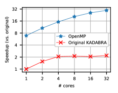
(a) Average speedup (preprecessing + ADS, geom. mean) of OpenMP baseline over the original sequential implementation of KADABRA

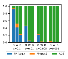
(b) Breakdown of sequential KADABRA running times into preprocessing and ADS (in percent) on instances orkut-links (O), wikipedia_link_de (W), and dimacs9-COL (D)

Figure 2: Performance of OpenMP baseline

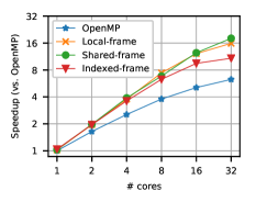
(a) Average ADS speedup (geom. mean) of epoch-based algorithms over sequential OpenMP baseline

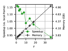
(b) Average ADS speedup (over 36-core local-frame, geom. mean) and memory consumption of shared-frame, depending on the number of SFs

Figure 3: Performance of epoch-based algorithms

The platform we use for our experiments is a Linux server equipped with 1.5TB RAM and two Intel Xeon Gold 6154 CPUs with 18 cores (for a total of 36 cores) at 3.00GHz. Each thread of the algorithm is pinned to a unique core; hyperthreading is disabled. Our implementation is written in C++ building upon the NetworKit toolkit [26]. We use 27 undirected real-world graphs in the experiments (see Appendix 0.E for more details). The error probability for KADABRA is set to $\delta=0.1$ for all experiments. Absolute running times of our experiments are reported in Appendix 0.F.

In a first experiment, we compare our OpenMP baseline against the original implementation of KADABRA (see Section 2.4 for these two approaches). We set the absolute approximation error to $\epsilon=0.01$. The overall speedup (i. e., both preprocessing and ADS) is reported in Figure 2(a). The results show that our OpenMP baseline outperforms the original implementation considerably (i. e., by a factor of $\numprint{6.89846099713451}\times$), even in a single-core setting. This is mainly due to implementation tricks (see Appendix 0.C.1) and parameter tuning (as discussed in Appendix 0.C.2). Furthermore, for 32 cores, our OpenMP baseline performs $\numprint{13.544344311728693}\times$ better than the original impelementation of KADABRA – or $\numprint{22.66442436431893}\times$ if only the ADS phase is considered. Hence, for the remaining experiments, we discard the original implementation as a competitor and focus on the parallel speedup of our algorithms.

To understand the relation between the preprocessing and ADS phases of KADABRA, we break down the running times of the OpenMP baseline in Figure 2(b). In this figure, we present the fraction of time that is spent in ADS on three exemplary instances and for different values of $\epsilon$. Especially if $\epsilon$ is small, the ADS running time dominates the overall performance of the algorithm. Thus, improving the scalability of the ADS phase is of critical importance. For this reason, we neglect the preprocessing phase and only consider ADS when comparing to our local-frame and shared-frame algorithms.

In Figure 3(a), we report the parallel speedup of the ADS phase of our epoch-based algorithms relative to the OpenMP baseline. All algorithms are configured to check the stopping condition after a fixed number of samples (see Appendix 0.C.3 for details). The number $F$ of SF pairs of shared-frame has been configured to $2$, which we found to be a good setting for $T=32$. On 32 cores, local-frame and shared-frame achieve parallel speedups of $\numprint{15.879639123178466}\times$ and $\numprint{18.081267115073295}$; they both significantly improve upon the OpenMP baseline, which can only achieve a parallel speedup of $\numprint{6.27616521473421}\times$ (i. e., local-frame and shared-frame are $\numprint{2.5301499530156892}\times$ and $\numprint{2.8809418644086824}\times$ faster, respectively; they also outperform the original implementation by factors of $\numprint{57.34439224050918}$ and $\numprint{65.29488898389054}$, respectively). The difference between local-frame and shared-frame is insignificant for lower numbers of cores; this is explained by the fact that the reduced memory footprint of shared-frame only improves performance once memory bandwidth becomes a bottleneck. For the same reason, both algorithms scale very well until 16 cores; due to memory bandwidth limitations, this nearly ideal scalability does not extend to 32 cores. This bandwidth issue is known to affect graph traversal algorithms in general [2, 15].

The indexed-frame algorithm is not as fast as local-frame and shared-frame on the instances depicted in Figure 3(a): it achieves a parallel speedup of $\numprint{10.818961592817336}\times$ on 32 cores. However, it is still considerably faster than the OpenMP baseline (by a factor of $\numprint{1.7238172072682618}\times$). There are two reasons why the determinism of indexed-frame is costly: index-frame has similar bandwidth requirements as local-frame; however, it has to allocate more memory as SFs are buffered for longer periods of time. On the other hand, even when enough samples are collected, the stopping condition has to be checked on older samples first, while local-frame and shared-frame can just check the stopping condition on the most recent sampling state.

In a final experiment, we evaluate the impact of the parameter $F$ of shared-frame on its performance. Figure 3(b) depicts the results. The experiment is done with 36 cores; hence memory pressure is even higher than in the previous experiments. The figure demonstrates that in this situation, minimizing the memory bandwith requirements at the expense of synchronization overhead is a good strategy. Hence for larger numbers of cores, we can minimize memory footprint and maximize performance at the same time.

5 Related Work

Our parallelization strategy can be applied to arbitrary ADS algorithms. ADS was first introduced by Lipton and Naughton to estimate the size of the transitive closure of a digraph [14]. It is used in a variety of fields, e. g., in statistical learning [23]. In the context of BC, ADS has been used to approximate distances between pairs of vertices of a graph [22], to approximate the BC values of a graph [3, 25, 6] and to approximate the BC value of a single vertex [9]. An analogous strategy is exploited by Mumtaz and Wang [21] to find approximate solutions to the group betweenness maximization problem.

Regarding more general (i. e., not necessarily ADS) algorithms for BC, a survey from Matta et al. [17] provides a detailed overview of the the state of the art. The RK [24] algorithm represents the leading non-adaptive sampling algorithm for BC approximation; KADABRA was shown to be 100 times faster than RK in undirected real-world graphs, and 70 times faster than RK in directed graphs[6]. McLaughlin and Bader [19] introduced a work-efficient parallel algorithm for BC approximation, implemented for single- and multi-GPU machines. Madduri et al. [16] presented a lock-free parallel algorithm optimized for specific architectures to approximate or compute BC exactly in massive networks.

The SFs used by our algorithms are concurrent data structures that enable us to minimize the synchronization latencies in multithread environments. Devising concurrent (lock-free) data structures that scale over multiple cores is not trivial and much effort has been devoted to this goal [7, 20]. A well-known solution is the Read-Copy-Update mechanism (RCU); it was introduced to achieve high multicore scalability on read-mostly data structures [18], and was leveraged by several applications [1, 10]. Concurrent hash tables [11] are another popular example.

6 Conclusions and Future Work

In this paper, we found that previous techniques to parallelize ADS algorithms are insufficient to scale to large numbers of threads. However, significant speedups can be achieved by employing adequate concurrent data structures. Using such data structures and our epoch mechanism, we were able to devise parallel ADS algorithms that consistently outperform the state of the art but also achieve different trade-offs between synchronization costs, memory footprint and determinism of the results.

Regarding future work, a promising direction for our algorithms is parallel computing with distributed memory; here, the stopping condition could be checked via (asynchronous) reduction of the SFs. In the case of BC this, might yield a way to avoid bottlenecks for memory bandwidth on shared-memory systems.

Appendix 0.A The C11 memory model

As mentioned in Section 2.1, we work in the C11 memory model. The weakest operations in this model are load-relaxed and store-relaxed operations; those only guarantee the atomicity of the memory access (i. e., they guarantee that no tearing occurs) but no ordering at all. Hence, the order in which store-relaxed writes become visible to load-relaxed reads can differ from the order in which the stores and loads are performed by individual threads. load-acquire and store-release additionally do provide ordering guarantees: if thread $t$ writes a word $X$ to a given memory location using store-release and thread $t^{\prime}$ reads $X$ using load-acquire from the same memory location, then all store operations – whether atomic or not – done by thread $t$ before the store of $X$ become visible to all load operations done by thread $t^{\prime}$ after the load of $X$. We note that C11 defines even stronger ordering guarantees that we do not require in this paper. Furthermore, on a hardware level, x86_64 implements a stronger total store order; thus, load-acquire and store-release compile to plain load and store instructions and our local-frame algorithm does not perform any synchronization instructions on x86_64.

Appendix 0.B Details of KADABRA Algorithm

In Section 2.3 we described the KADABRA algorithm; in this appendix, we illustrate the stopping condition more in detail and show that evaluating it in a consistent state is crucial for the correctness of the algorithm. The functions $f$ and $g$ we mentioned in Eq. 1 are defined as [6]:

$$f(\widetilde{\mathbf{b}}(v),\delta_{L}(v),\omega,\tau) =\frac{1}{\tau}\left(\log\frac{1}{\delta_{L}(v)}\right)\left(\frac{1}{3}-\frac{\omega}{\tau}+\sqrt{\left(\frac{1}{3}-\frac{\omega}{\tau}\right)^{2}+\frac{2\widetilde{\mathbf{b}}(v)\omega}{\log\frac{1}{\delta_{L}(v)}}}\right)$$

$$g(\widetilde{\mathbf{b}}(v),\delta_{U}(v),\omega,\tau) =\frac{1}{\tau}\left(\log\frac{1}{\delta_{U}(v)}\right)\left(\frac{1}{3}+\frac{\omega}{\tau}+\sqrt{\left(\frac{1}{3}+\frac{\omega}{\tau}\right)^{2}+\frac{2\widetilde{\mathbf{b}}(v)\omega}{\log\frac{1}{\delta_{U}(v)}}}\right)$$

where $\widetilde{\mathbf{b}}(v)$ is the approximation of the BC of vertex $v$ obtained after $\tau$ samples. When the stopping condition is evaluated, $f$ and $g$ are computed for every vertex of the graph and the algorithm terminates if:

$$f(\widetilde{\mathbf{b}}(v),\delta_{L}(v),\omega,\tau)\leq\epsilon\quad\text{and}\quad g(\widetilde{\mathbf{b}}(v),\delta_{U}(v),\omega,\tau)\leq\epsilon$$

holds for every vertex $v$ of the graph. It is straightforward to verify that both $f$ and $g$ grow with $\widetilde{\mathbf{b}}(v)$ but that $g$ decreases with $\tau$. Thus, evaluating the stopping condition with inconsistent data (e. g., if accesses to $\tau$ and $\widetilde{\mathbf{b}}(v)$ are not synchronized) could lead to an erroneous termination of the algorithm.

Appendix 0.C Optimization and Tuning

0.C.1 Improvements to the KADABRA Implementation

In the following we document some improvements to the sequential KADABRA implementation of Borassi and Natale [6]. First, we avoid searching for non-existing shortest paths between a pair $(s,t)$ of selected vertices by checking if $s$ and $t$ belong to the same connect component. Then, we reduce the memory footprint of the sampling procedure: the original KADABRA implementation stores all predecessors on shortest paths in a separate graph $G^{\prime}$, which is used to backtrack the path starting from the last explored vertices. Our implementation avoids the use of $G^{\prime}$ by reconstructing shortest $s$-$t$-paths from the original graph $G$ and a distance vector. Furthermore, for each shortest $s$-$t$-path sampled, the original KADABRA implementation needs to reset a Boolean “visited” array with an overall additional cost of $\Theta(|V|)$ time per sample. We avoid doing this by using 7 bits per element in this array to store a timestamp that indicates when the vertex was last visited; therefore, the array needs to be reset only once in $2^{7}=128$ BFSs.

0.C.2 Balancing Costs of Termination Checks

Although the pseudocode of Algorithms 1 and 2 checks the stopping condition after every sample, this amount of checking is excessive in practice. Hence, both the original KADABRA and the OpenMP ADS algorithms check the stopping condition after a fixed number $N$ of samples. $N$ represents a tradeoff between the time required to check the stopping condition and the time required to sample a shortest path. In the original KADABRA implementation, $N$ is set to 11; however, this choice turned out to be inefficient in our experiments. Thus, we formed a small set of the instances for parameter tuning and ran experiments with different values of $N$. As the result, we found that $N=1000$ empirically performs best.

0.C.3 Termination Latency in Epoch-based Approach

In the epoch-based approach, we also need to balance the frequency of checking the stopping condition and the time invested into sampling; however, we face a different problem: the accumulation of all SFs before the stopping condition is checked takes $\mathcal{O}(Tn)$ time, thus the length of an epoch depends on $T$ (see Section 3.3). This is an undesirable artifact as it introduces an additional delay between the time when the algorithm could potentially stop (because enough samples have been collected) and the time when the algorithm actually stops (because the accumulation is completed). It would be preferable to check the stopping condition after a constant number of samples (summed over all threads) – as the sequential and OpenMP variants naturally do.

While it seems unlikely that a constant number of samples per epoch can be achieved (without additional synchronization overhead), we aim to satisfy this property heuristically. Checking the stopping condition after $N_{0}=(1/T)N$ samples per thread seems to be a reasonable heuristic. However, it does not account for the fact that only one thread performs the check while all additional threads continue to sample data. Thus, we check the stopping condition after

$$N_{0}=\frac{1}{T^{\xi}}N$$

samples from thread 0. Here, $\xi$ is another parameter that can be tuned. Using the same approach as in Appendix 0.C.2 (and running the algorithm on 32 cores), we empirically determined $\xi=\log_{32}(N/10)\approx 1.33$ to be a good choice.

Appendix 0.D Details on Epoch-Based Algorithms

0.D.1 Visualization of Epoch Transition

Figure 4: Transition after $\mathtt{epochToRead}$ is set to $5$. Thread 2 already writes to the SF of epoch 6 (using the $f_{\mathrm{sam}}$ pointer). Thread 9 still writes to the SF of epoch 5 but advances to epoch 6 once it checks $\mathtt{epochToRead}$ (dashed orange line). Afterwards, thread 9 publishes its SF of epoch 5 to $\mathtt{sfFin}$ (dashed blue line). Finally, the stopping condition is checked using both SFs of epoch 5 (i. e., the SFs now pointed to by $\mathtt{sfFin}$).

Figure 4 visualizes the update of the $\mathtt{sfFin}$ pointers after an epoch transition is initiated by incrementing $\mathtt{epochToRead}$. The exact mechanism is discussed in Section 3.1

0.D.2 Indexed-frame Algorithm

(a) SF indices in indexed-frame algorithm (not to be confused with epoch numbers).

(b) Reservation of SFs for $a=2$. Thread 0 (blue) has finished SFs with indices $T$, $2T$, $3T$ and $4T$. Because thread 1 (red) did not finish SF $T+1$ yet, thread 0 reserves indices $2T+1$ and $3T+1$.

Figure 5: Indices of SFs in indexed-frame algorithm. Central numbers indicate SF indices. Numbers in bottom right corners (and colors) denote the thread that will compute the SF. Dashed SFs are already finished.

In this subsection, we introduce the indexed-frame algorithm that is a variant of local-frame but always obtains deterministic results. In particular, we highlight the modifications compared to local-frame that are necessary to avoid non-determinism.

There are two sources of non-determinism in the epoch-based algorithms: First, because threads generate random numbers independently from each other and the pseudo-random number generator (PRNG) of each thread is seeded differently, the sequence of generated random numbers depends on the number of threads. Secondly, and more importantly, the point in time where a thread notices that the stopping condition needs to be checked (i. e., $\mathtt{epochToRead}$ is read in line 7 of Algorithm 2) is non-deterministic. Thus, among multiple executions of the algorithm, the SFs that are checked differ in the number of samples and in the PRNG state used to generate the samples.

Indexed-frame avoids the first problem by re-seeding the random number generator of each thread whenever the thread moves to a new epoch. To avoid a dependence on the number of threads, the new seed should only vary based on a unique index of the generated SF (not to be confused with the epoch number). As an index for the SF of epoch $e$, we choose $(eT+t)$, as every thread $t$ contributes exactly one SF to each epoch $e$. This scheme is depicted in Figure 5(a).

Handling the second issue turns out to be more involved. As we need to ensure that the stopping condition is always checked on exactly the same SFs, the point in time where a thread moves to a new epoch must be independent of the time when the stopping condition is checked. To achieve that, indexed-frame writes a fixed number of samples to each SF. That, however, means that by the time a check is performed, a thread can have finished multiple SFs. To deal with multiple finished SFs, we use a per-thread queue of SFs which have already been finished but which were not considered by the stopping condition yet. While the size of this queue is unbounded in theory, in our experiments we never observed a thread buffering more than 12 SFs at a time (with an average of 3 SFs allocated per thread); thus, we do not implement a sophisticated strategy to bound the queue length. The following subsection, however, discusses such a strategy for ADS algorithms where this becomes a problem.

0.D.3 Bounded Memory Complexity in Indexed-frame

As our experiments demonstrated, the SF buffering overhead of the deterministic algorithm is not problematic in practice. However, at the cost of additional synchronization, it is possible to also bound the theoretical memory complexity the algorithm. In particular, if there are lower and upper bounds $\mathcal{C}_{\ell}$ and $\mathcal{C}_{u}$ on the time to compute a single SF, we can reserve SF indices to bound the number of simultaneously allocated SFs: instead of computing the SFs with indices $(t,t+T,t+2T,\ldots)$, each thread $t$ determines (by synchronizing with all other threads) the smallest index $i$ of a SF that is not reserved yet (see Figure 5(b) as an illustration of this process). Then, the SFs with indices $(i,i+T,i+2T,\ldots,i+aT)$ for some constant $a$ are reserved by $t$ and $t$ computes exactly those SFs before doing another reservation. The bounds on the computation time of a single SF imply that all other threads can only perform a constant number $\mathcal{C}_{u}/\mathcal{C}_{\ell}$ of reservations until an epoch is finished (and all SFs of the epoch can be reclaimed). The constant $a$ can be chosen to balance the maximal number of buffered SFs and synchronization costs required for reservation.

Appendix 0.E List of Instances

Table 1: List of instances used for the experiments.

Network name	# of vertices	# of edges	Diameter	Category
tntp-ChicagoRegional	12,979	20,627	106	Infrastructure
dimacs9-NY	264,346	365,050	720	Infrastructure
dimacs9-COL	435,666	521,200	1,255	Infrastructure
munmun_twitter_social	465,017	833,540	8	Social
com-amazon	334,863	925,872	47	Co-purchase
loc-gowalla_edges	196,591	950,327	16	Social
web-NotreDame	325,729	1,090,108	46	Hyperlink
roadNet-PA	1,088,092	1,541,898	794	Infrastructure
roadNet-TX	1,379,917	1,921,660	1,064	Infrastructure
web-Stanford	281,903	1,992,636	753	Hyperlink
petster-dog-household	256,127	2,148,179	11	Social
flixster	2,523,386	7,918,801	8	Social
as-skitter	1,696,415	11,095,298	31	Computer
dbpedia-all	3,966,895	12,610,982	146	Relationship
actor-collaboration	382,219	15,038,083	13	Collaboration
soc-pokec-relationships	1,632,803	22,301,964	14	Social
soc-LiveJournal1	4,846,609	42,851,237	20	Social
livejournal-links	5,204,175	48,709,621	23	Social
wikipedia_link_ceb	7,891,015	63,915,385	9	Hyperlink
wikipedia_link_ru	3,370,462	71,950,918	10	Hyperlink
wikipedia_link_sh	3,924,218	76,439,386	9	Hyperlink
wikipedia_link_de	3,603,726	77,546,982	14	Hyperlink
wikipedia_link_it	2,148,791	77,875,131	9	Hyperlink
wikipedia_link_sv	6,100,692	99,864,874	10	Hyperlink
wikipedia_link_fr	3,333,397	100,461,905	10	Hyperlink
wikipedia_link_sr	3,175,009	103,310,837	10	Hyperlink
orkut-links	3,072,441	117,184,899	10	Social

Appendix 0.F Detailed Experimental Data

In this appendix we show the detailed running time of our algorithms on every instance. For better readability, we partitioned the instances into two categories: moderate instances achieved a total running time of less than 100 seconds (Table 2); the others are shown in Table 3.

Table 2: Absolute running times (s) on moderate instances. Total: ADS with preprocessing on a single core.

(a) OMP: OpenMP baseline, L: local-frame

Network Name		1 core		2 cores		4 cores		8 cores		16 cores		32 cores
	Total	OMP	L	OMP	L	OMP	L	OMP	L	OMP	L	OMP	L
tntp-ChicagoRegional	6.70	6.62	5.66	3.25	2.83	1.56	1.37	0.85	0.66	0.45	0.33	0.27	0.16
munmun_twitter_social	7.99	1.72	1.49	1.41	0.83	1.09	0.45	0.89	0.24	0.84	0.23	0.78	0.17
com-amazon	10.49	9.47	9.18	4.47	4.38	3.02	2.35	2.27	1.34	1.94	0.86	1.41	0.54
loc-gowalla_edges	2.82	2.50	2.09	1.49	0.99	1.11	0.49	0.87	0.20	0.70	0.11	0.67	0.10
web-NotreDame	7.66	7.33	6.55	4.34	3.30	3.17	1.72	2.50	0.68	2.14	0.43	1.93	0.33
web-Stanford	34.62	33.87	29.95	15.76	15.54	11.62	7.95	7.96	2.79	5.49	1.75	4.48	1.33
petster-dog-household	5.31	4.83	3.89	2.67	2.12	1.82	1.09	1.43	0.67	1.30	0.56	1.32	0.42
flixster	13.99	10.94	10.03	7.87	5.77	6.61	3.20	5.49	1.91	4.90	1.32	4.78	1.32
as-skitter	17.14	13.76	13.16	9.85	7.57	7.33	3.99	5.80	2.55	5.14	1.77	5.11	2.21
actor-collaboration	8.69	5.87	6.21	3.88	3.18	2.60	1.96	1.82	1.16	1.41	0.68	1.09	0.54
soc-pokec-relationships	25.38	16.57	18.21	10.37	9.00	8.00	5.23	6.07	3.02	5.28	2.56	5.40	2.08
soc-LiveJournal1	54.91	36.52	39.08	31.53	22.37	22.29	11.68	17.79	6.12	15.57	4.69	14.82	4.03
livejournal-links	62.27	46.19	44.52	31.16	24.99	23.49	13.43	18.11	7.57	15.46	4.90	15.51	4.33
wikipedia_link_sh	41.54	21.68	17.98	17.43	9.49	14.74	4.68	13.13	2.44	12.36	2.05	12.08	2.11
wikipedia_link_sr	56.30	45.55	42.66	32.21	21.83	20.28	10.69	15.63	6.08	12.92	3.72	12.73	2.69

(b) S: shared-frame, I: indexed-frame

Network Name		1 core		2 cores		4 cores		8 cores		16 cores		32 cores
	Total	S	I	S	I	S	I	S	I	S	I	S	I
tntp-ChicagoRegional	6.70	6.71	5.48	3.30	2.75	1.48	1.38	0.64	0.70	0.31	0.43	0.15	0.29
munmun_twitter_social	7.99	1.51	1.60	0.80	0.90	0.45	0.49	0.28	0.29	0.20	0.17	0.19	0.23
com-amazon	10.49	8.44	8.88	4.04	4.21	2.34	2.52	1.43	1.48	0.78	1.22	0.42	0.89
loc-gowalla_edges	2.82	2.23	2.34	0.79	1.11	0.46	0.53	0.28	0.31	0.14	0.17	0.08	0.11
web-NotreDame	7.66	6.34	6.81	3.18	3.52	1.40	1.58	0.76	0.99	0.52	0.66	0.22	0.60
web-Stanford	34.62	28.81	29.51	14.27	14.01	5.73	8.68	4.41	5.50	1.80	2.13	1.18	1.50
petster-dog-household	5.31	4.24	3.68	2.21	1.95	1.05	1.14	0.66	0.75	0.62	0.78	0.46	0.73
flixster	13.99	10.30	11.02	6.03	6.00	3.01	3.31	2.25	1.97	1.36	1.45	1.33	1.90
as-skitter	17.14	13.26	14.23	7.59	8.13	4.11	4.42	2.42	2.44	1.50	2.08	1.13	1.74
actor-collaboration	8.69	6.28	5.48	3.28	3.27	1.85	1.71	1.06	1.03	0.68	0.69	0.48	1.01
soc-pokec-relationships	25.38	16.22	17.18	8.77	9.38	5.57	5.79	3.40	2.98	2.15	2.00	1.40	2.49
soc-LiveJournal1	54.91	35.60	40.49	22.70	18.93	13.13	14.15	7.04	8.28	4.69	6.32	3.29	5.72
livejournal-links	62.27	44.49	44.85	25.44	24.65	12.45	15.29	7.69	8.53	5.07	6.89	3.77	6.95
wikipedia_link_sh	41.54	17.94	21.49	9.81	11.86	4.89	7.04	2.78	3.88	1.96	1.68	1.55	2.26
wikipedia_link_sr	56.30	45.93	41.54	24.91	23.70	11.36	13.18	7.09	6.54	4.44	5.11	2.95	5.23

Table 3: Absolute running times (s) on expensive instances. Total: ADS with preprocessing on a single core.

(a) OMP: OpenMP baseline, L: local-frame

Network Name		1 core		2 cores		4 cores		8 cores		16 cores		32 cores
	Total	OMP	L	OMP	L	OMP	L	OMP	L	OMP	L	OMP	L
dimacs9-NY	249	246	212	97	106	54	55	30	28	19	14	10	6
dimacs9-COL	405	397	358	177	177	101	94	55	47	30	23	17	11
roadNet-PA	1,961	1,937	1,851	1,027	942	521	458	284	235	148	121	92	59
roadNet-TX	1,965	1,937	2,001	1,042	1,035	544	496	279	250	165	130	89	64
dbpedia-all	412	402	395	227	215	126	80	76	42	54	22	41	19
wikipedia_link_ceb	1,337	1,272	1,435	701	707	415	307	238	160	156	98	121	74
wikipedia_link_ru	142	126	132	89	73	52	44	36	23	26	12	24	12
wikipedia_link_de	155	145	182	106	100	54	57	37	21	25	12	20	13
wikipedia_link_it	152	112	145	82	70	58	41	27	24	20	14	16	9
wikipedia_link_sv	444	423	472	258	255	160	105	105	61	73	32	60	31
wikipedia_link_fr	194	168	177	131	106	75	58	41	30	32	14	24	12
orkut-links	206	107	110	66	64	44	35	27	19	19	10	15	9

(b) S: shared-frame, I: indexed-frame

Network Name		1 core		2 cores		4 cores		8 cores		16 cores		32 cores
	Total	S	I	S	I	S	I	S	I	S	I	S	I
dimacs9-NY	249	198	203	95	101	49	53	26	31	13	14	6	9
dimacs9-COL	405	345	339	177	171	94	93	50	49	22	25	11	17
roadNet-PA	1,961	1,975	1,781	998	950	471	463	242	252	113	151	60	82
roadNet-TX	1,965	1,994	1,943	1,022	1,038	504	514	232	277	119	165	63	89
dbpedia-all	412	411	391	214	205	96	83	49	66	18	25	14	36
wikipedia_link_ceb	1,337	1,421	1,268	691	665	370	399	158	162	86	135	68	117
wikipedia_link_ru	142	134	125	67	69	42	35	25	26	14	19	11	16
wikipedia_link_de	155	155	170	80	98	39	56	24	32	12	19	8	15
wikipedia_link_it	152	120	129	74	68	38	45	21	26	11	20	10	16
wikipedia_link_sv	444	438	429	272	246	111	108	55	58	30	46	24	54
wikipedia_link_fr	194	181	168	96	92	55	60	30	35	15	29	14	20
orkut-links	206	119	107	60	66	34	37	19	25	10	20	7	15

References

- [1] Arbel, M., Attiya, H.: Concurrent updates with rcu: search tree as an example. In: Proceedings of the 2014 ACM symposium on Principles of distributed computing. pp. 196–205. ACM (2014)
- [2] Bader, D.A., Cong, G., Feo, J.: On the architectural requirements for efficient execution of graph algorithms. In: Parallel Processing, 2005. ICPP 2005. International Conference on. pp. 547–556. IEEE (2005)
- [3] Bader, D.A., Kintali, S., Madduri, K., Mihail, M.: Approximating betweenness centrality. In: International Workshop on Algorithms and Models for the Web-Graph. pp. 124–137. Springer (2007)
- [4] Boldi, P., Vigna, S.: Axioms for centrality. Internet Mathematics 10(3-4), 222–262 (2014). https://doi.org/10.1080/15427951.2013.865686
- [5] Borassi, M., Crescenzi, P., Habib, M.: Into the square: On the complexity of some quadratic-time solvable problems. Electr. Notes Theor. Comput. Sci. 322, 51–67 (2016). https://doi.org/10.1016/j.entcs.2016.03.005, https://doi.org/10.1016/j.entcs.2016.03.005
- [6] Borassi, M., Natale, E.: KADABRA is an adaptive algorithm for betweenness via random approximation. In: 24th Annual European Symposium on Algorithms, ESA 2016, August 22-24, 2016, Aarhus, Denmark. pp. 20:1–20:18 (2016). https://doi.org/10.4230/LIPIcs.ESA.2016.20
- [7] Boyd-Wickizer, S., Clements, A.T., Mao, Y., Pesterev, A., Kaashoek, M.F., Morris, R., Zeldovich, N., et al.: An analysis of linux scalability to many cores. In: OSDI. vol. 10, pp. 86–93 (2010)
- [8] Brandes, U.: A faster algorithm for betweenness centrality. Journal of mathematical sociology 25(2), 163–177 (2001)
- [9] Chehreghani, M.H., Bifet, A., Abdessalem, T.: Novel adaptive algorithms for estimating betweenness, coverage and k-path centralities. CoRR abs/1810.10094 (2018), http://arxiv.org/abs/1810.10094
- [10] Clements, A.T., Kaashoek, M.F., Zeldovich, N.: Scalable address spaces using rcu balanced trees. ACM SIGPLAN Notices 47(4), 199–210 (2012)
- [11] David, T., Guerraoui, R., Trigonakis, V.: Everything you always wanted to know about synchronization but were afraid to ask. In: ACM SIGOPS 24th Symposium on Operating Systems Principles, SOSP ’13, Farmington, PA, USA, November 3-6, 2013. pp. 33–48 (2013). https://doi.org/10.1145/2517349.2522714
- [12] Gonzalez, T.F.: Handbook of Approximation Algorithms and Metaheuristics (Chapman & Hall/Crc Computer & Information Science Series). Chapman & Hall/CRC (2007)
- [13] ISO: ISO/IEC 14882:2011 Information technology — Programming languages — C++. International Organization for Standardization, Geneva, Switzerland (Feb 2012), http://www.iso.org/iso/iso_catalogue/catalogue_tc/catalogue_detail.htm?csnumber=50372
- [14] Lipton, R.J., Naughton, J.F.: Estimating the size of generalized transitive closures. In: Proceedings of the 15th Int. Conf. on Very Large Data Bases (1989)
- [15] Lumsdaine, A., Gregor, D., Hendrickson, B., Berry, J.: Challenges in parallel graph processing. Parallel Processing Letters 17(01), 5–20 (2007)
- [16] Madduri, K., Ediger, D., Jiang, K., Bader, D.A., Chavarria-Miranda, D.: A faster parallel algorithm and efficient multithreaded implementations for evaluating betweenness centrality on massive datasets. In: Parallel & Distributed Processing, 2009. IPDPS 2009. IEEE International Symposium on. pp. 1–8. IEEE (2009)
- [17] Matta, J., Ercal, G., Sinha, K.: Comparing the speed and accuracy of approaches to betweenness centrality approximation. Computational Social Networks 6(1), 2 (2019)
- [18] McKenney, P.E., Slingwine, J.D.: Read-copy update: Using execution history to solve concurrency problems. In: Parallel and Distributed Computing and Systems. pp. 509–518 (1998)
- [19] McLaughlin, A., Bader, D.A.: Scalable and high performance betweenness centrality on the gpu. In: Proceedings of the International Conference for High performance computing, networking, storage and analysis. pp. 572–583. IEEE Press (2014)
- [20] Michael, M.M.: Hazard pointers: Safe memory reclamation for lock-free objects. IEEE Transactions on Parallel & Distributed Systems (6), 491–504 (2004)
- [21] Mumtaz, S., Wang, X.: Identifying top-k influential nodes in networks. In: Proceedings of the 2017 ACM on Conference on Information and Knowledge Management. pp. 2219–2222. ACM (2017)
- [22] Oktay, H., Balkir, A.S., Foster, I., Jensen, D.D.: Distance estimation for very large networks using mapreduce and network structure indices. In: Workshop on Information Networks (2011)
- [23] Provost, F., Jensen, D., Oates, T.: Efficient progressive sampling. In: Proceedings of the fifth ACM SIGKDD international conference on Knowledge discovery and data mining. pp. 23–32. ACM (1999)
- [24] Riondato, M., Kornaropoulos, E.M.: Fast approximation of betweenness centrality through sampling. Data Mining and Knowledge Discovery 30(2), 438–475 (2016)
- [25] Riondato, M., Upfal, E.: Abra: Approximating betweenness centrality in static and dynamic graphs with rademacher averages. ACM Transactions on Knowledge Discovery from Data (TKDD) 12(5), 61 (2018)
- [26] Staudt, C.L., Sazonovs, A., Meyerhenke, H.: Networkit: A tool suite for large-scale complex network analysis. Network Science 4(4), 508–530 (2016)