Rods and Rings: Soft Subdivision Planner for ${\mathbb{R}}^{3}\times S^{2}$

Abstract

We consider path planning for a rigid spatial robot moving amidst polyhedral obstacles. Our robot is either a rod or a ring. Being axially-symmetric, their configuration space is ${\mathbb{R}}^{3}\times S^{2}$ with 5 degrees of freedom (DOF). Correct, complete and practical path planning for such robots is a long standing challenge in robotics. While the rod is one of the most widely studied spatial robots in path planning, the ring seems to be new, and a rare example of a non-simply-connected robot. This work provides rigorous and complete algorithms for these robots with theoretical guarantees. We implemented the algorithms in our open-source Core Library. Experiments show that they are practical, achieving near real-time performance. We compared our planner to state-of-the-art sampling planners in OMPL [30].

Our subdivision path planner is based on the twin foundations of $\varepsilon$-exactness and soft predicates. Correct implementation is relatively easy. The technical innovations include subdivision atlases for $S^{2}$, introduction of $\Sigma_{2}$ representations for footprints, and extensions of our feature-based technique for “opening up the blackbox of collision detection”.

1 Introduction

Motion planning [17, 5] is a fundamental topic in robotics because the typical robot is capable of movement. Such algorithms are increasingly relevant with the current surge of interest in inexpensive commercial mobile robots, from domestic robots that vacuum the floor to drones that deliver packages. We focus on what is called path planning which, in its elemental form, asks for a collision-free path from a start to a goal position, assuming a known environment. Path planning is based on robot kinematics and collision-detection only, and the variety of such problems are surveyed in [14]. The output of a “path planner” is either a path or a NO-PATH, signifying that no path exists. Remarkably, the single bit of information encoded by NO-PATH is often missing in discussions. The standard definitions of correctness for path planners (resolution completeness and probabilistic completeness) omit this bit [31]. The last 30 years have seen a flowering of practical path planning algorithms. The dominant algorithmic paradigm of these planners has been variants of the Sampling Approach such as PRM, EST, RRT, SRT, etc (see [5, p. 201]). Because this bit of information is not built into the specification of such algorithms, it has led to non-termination issues and a large literature addressing the “narrow passage problem” (e.g., [21, 8]). Our present paper is based on the Subdivision Approach. This approach has a venerable history in robotics – see [3, 39] for early planners based on subdivision.

Exact path planning has many issues including a serious gap between theory and implementability. In [31, 32], we introduced a theoretical framework based on subdivision to close this gap. This paper demonstrates for the first time that our framework is able to achieve rigorous state-of-the-art planners in 3D. Figure 1 shows our rod robot in an environment with 100 random tetrahedra. Figure 6 shows our ring robot in an environment with pillars and L-shaped posts. See a video demo from http://cs.nyu.edu/exact/gallery/rod-ring/rod_ring.html.

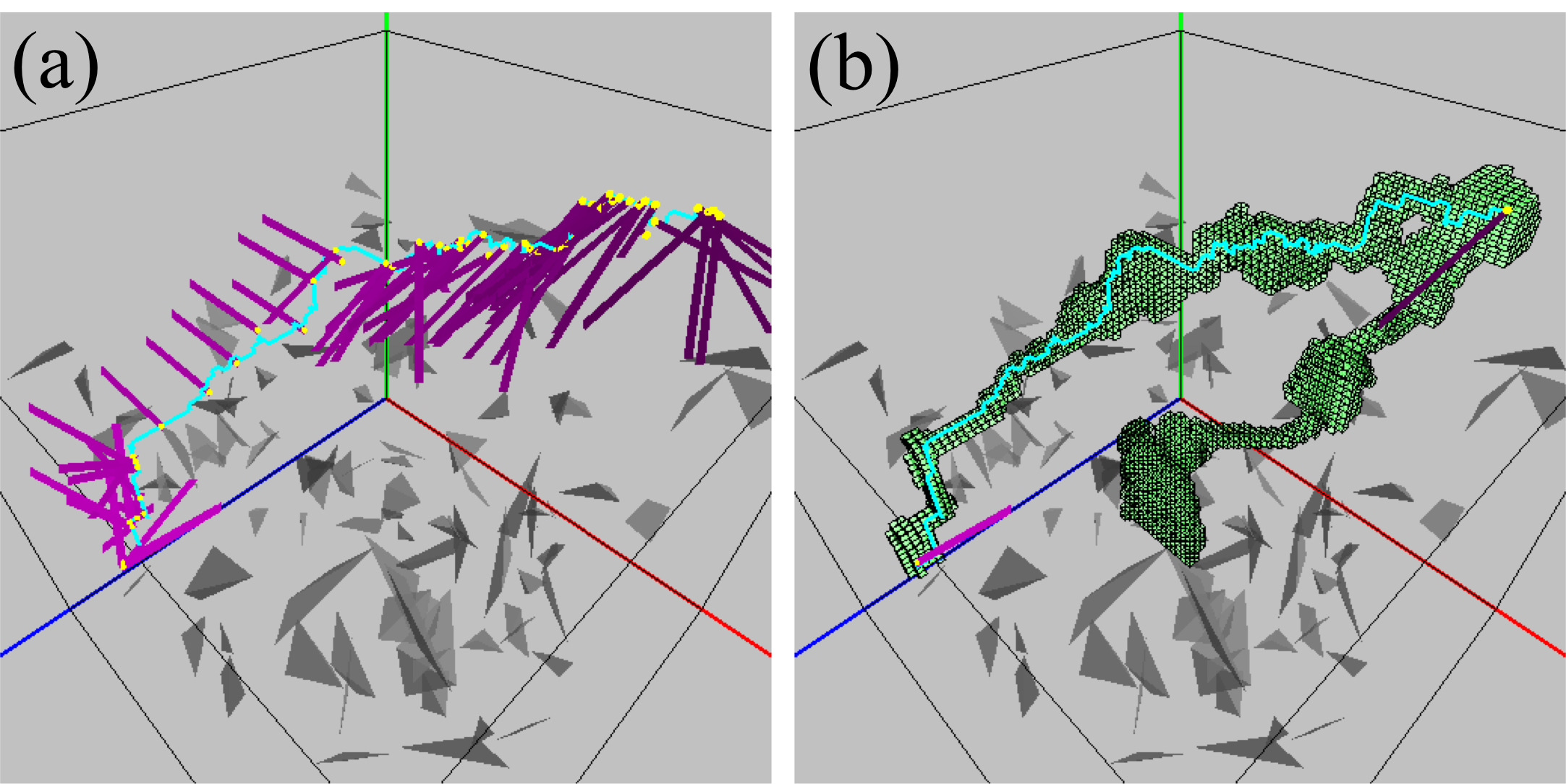
Figure 1: Rod robot amidst 100 random tetrahedra: (a) trace of a found path; (b) subdivision of translational boxes on the path.

In this paper, we consider a rigid spatial robot $R_{0}$ that has an axis of symmetry. See Figure 2(a) for several possibilities for $R_{0}$: rod (“ladder”), cone (“space shuttle”), disc (“frisbee”) and ring (“space station”). Our techniques easily allow these robots to be “thickened” by Minkowski sum with balls (see [34]). The configuration space may be taken to be $C_{space}={\mathbb{R}}^{3}\times S^{2}$ where $S^{2}$ is the unit $2$-sphere. We identify $R_{0}$ with a closed subset of ${\mathbb{R}}^{3}$, called its “canonical footprint”. E.g., if $R_{0}$ is a rod (resp., ring), then the canonical footprint is a line segment (resp., circle) in ${\mathbb{R}}^{3}$. Each configuration $\gamma\in C_{space}$ corresponds to a rotated translated copy of the canonical footprint, which we denote by $F\!p(\gamma)$. Path planning involves another input, the obstacle set $\Omega\subseteq{\mathbb{R}}^{3}$ that the robot must avoid. We assume that $\Omega$ is a closed polyhedral set. Say $\gamma$ is free if $F\!p(\gamma)\cap\Omega$ is empty. The free space comprising all the free configurations is an open set by our assumptions, and is denoted $C_{free}=C_{free}(\Omega)$. A parametrized continuous curve $\mu:[0,1]\to C_{space}$ is called a path if the range of $\mu$ is in $C_{free}$. Path planning amounts to finding such paths. Following [39], we need to classify boxes $B\subseteq C_{space}$ into one of three types: $\mathtt{FREE}$, $\mathtt{STUCK}$ or $\mathtt{MIXED}$. Let $C(B)$ denote the classification of $B$: $C(B)=\mathtt{FREE}$ if $B\subseteq C_{free}$, and $C(B)=\mathtt{STUCK}$ if $B$ is in the interior of $C_{space}\setminus C_{free}$. Otherwise, $C(B)=\mathtt{MIXED}$. One of our goals is to introduce classifications $\widetilde{C}(B)$ that are “soft versions” of $C(B)$ (see Appendix A).

Figure 2: (a) 3D rigid robots with $C_{space}={\mathbb{R}}^{3}\times S^{2}$. (b) Subdivision atlas for $S^{2}$ via ${\widehat{S^{2}}}$.

We present four desiderata in path planning:
(G0) the planner must be mathematically rigorous and complete;
(G1) it must have correct implementations which are also:
(G2) relatively easy to achieve and
(G3) practically efficient.
In (G0), we use the standard Computer Science notion of an algorithm being complete if (a) it is partially complete and (b) it halts. The notions of resolution completeness and probabilistic completeness in robotics have requirement (a) but not (b). In probabilistic-complete algorithms, halting with NO-PATH is achieved heuristically by putting limits on time and/or number of samples. But such limits are not intrinsic to the input instance. In resolution-complete algorithms, NO-PATH halting is based on width $w$ of subdivision box being small enough (say $w<\varepsilon$). One issue is that the width of a box is a direct measure of clearance (but there is a nontrivial correlation); secondly, box predicates are numerical and “accurate enough” ($\sigma$-effective in our theory). These issues are exacerbated when algorithms do not use box predicates, but perform sampling at grid points of the subdivision. In contrast, our NO-PATH guarantees an intrinsic property: there is no path of clearance $K\varepsilon$ (see below).

But desideratum (G0) is only the base line. A (G0)-planner may not be worth much in a practical area like robotics unless it also has implementations with properties (G1-G3). E.g., the usual exact algorithms satisfy (G0) but their typical implementations fail (G1). With proper methods [29], it is possible to satisfy (G1); Halperin et al [13] give such solutions in 2D using CGAL. Both (G0) and (G1) can be formalized (see next), but (G2) and (G3) are informal. The robotics community has developed various criteria to evaluate (G2) and (G3). The accepted practice is having an implementation (proving (G2)) that achieves “real time” performance on a suite of non-trivial instances (proving (G3)).

The main contribution of this paper is the design of planners for spatial robots with 5 DOFs that have the “good” properties (G0-G3). This seems to be the first for such robots. To achieve our results, we introduce theoretical innovations and algorithmic techniques that may prove to be more widely applicable.

In path planning and in Computational Geometry, there is a widely accepted interpretation of desideratum (G0): it is usually simply called “exact algorithms”. But to stress our interest in alternative notions of exactness, we refer to the standard notion as exact (unqualified). Planners that are exact (unqualified) are first shown in [25]; this can be viewed as a fundamental result on decidability of connectivity in semi-algebraic sets [1]. The curse of exact (unqualified) algorithms is that the algorithm must detect any degeneracies in the input and handle them explicitly. But exact (unqualified) algorithms are rare, mainly because degeneracies are numerous and hard to analyze: the usual expedient is to assume “nice” (non-degenerate) inputs. So the typical exact (unqualified) algorithms in the literature are conditional algorithms, i.e., its correctness is conditioned on niceness assumptions. Such gaps in exact (unqualified) algorithms are not an issue as long as they are not implemented. For non-linear problems beyond 2D, complete degeneracy analysis is largely non-existent. This is vividly seen in the fact that, despite long-time interest, there is still no exact (unqualified) algorithm for the Euclidean Voronoi diagram of a polyhedral set (see [15, 12, 11, 35]). For similar reasons, unconditional exact (unqualified) path planners in 3D are unknown.

We now address (G1-G3). The typical implementation is based on machine arithmetic (the IEEE standard), which may satisfy (G2) but almost certainly not (G1). We regard this as a (G1-G2) trade-off. In fact, our implementations here as well as in our previous papers [31, 19, 34] are such machine implementations. This follows the practice in the robotics community, in order to have a fair comparison against other implementations. Below, we shall expand on our claims about (G1-G3) including how to achieve theoretically correct implementation (G1). What makes this possible is our replacement of “exact (unqualified)” planners by “exact (up to resolution)” planners, defined below:

Resolution-Exact Path Planning for robot $R_{0}$: Input: $(\alpha,\beta,\Omega;B_{0},\varepsilon)$ where $\alpha,\beta\in C_{space}(R_{0})$ is the start and goal, $\Omega\subseteq{\mathbb{R}}^{3}$ the obstacle set, $B_{0}\subseteq C_{space}(R_{0})$ is a box, and $\varepsilon>0$. Output: Halt with either an $\Omega$-free path from $\alpha$ to $\beta$ in $B_{0}$, or NO-PATH satisfying the conditions (P) and (N) below.

The resolution-exact planner (or, $\varepsilon$-exact planner) has an accuracy constant $K>1$ (independent of input) such that its output satisfies two conditions:

• (P) If there is a path (from $\alpha$ to $\beta$ in $B_{0}$) of clearance $K\varepsilon$, the output must be a path.

• (N) If there is no path in $B_{0}$ of clearance $\varepsilon/K$, the output must be NO-PATH.

Here, clearance of a path is the minimum separation of the obstacle set $\Omega$ from the robot’s footprint on the path. Note that the preconditions for (P) and (N) are not exhaustive: in case the input fails both preconditions, our planner may either output a path or NO-PATH. This indeterminacy is essential to escape from exact computation (and arguably justified for robotics [32]). The constant $K>1$ is treated in more detail in [31, 33]. But resolution-exactness is just a definition. How do we design such algorithms? We propose to use subdivision, and couple with soft predicates to exploit resolution-exactness. We replace the classification $C(B)$ by a soft version $\widetilde{C}(B)$ [31]. This leads to a general resolution-exact planner which we call Soft Subdivision Search (SSS) [32, 33] that shares many of the favorable properties of sampling planners (and unlike exact planners). We demonstrated in [31, 19, 34] that for planar robots with up to 4 DOFs, our planners can consistently outperform state-of-the-art sampling planners.

1.1 What is New: Contributions of This Paper

In this work, we design $\varepsilon$-exact planners for rods and rings, with accompanying implementation that addresses the desiderata (G0-G3). This fulfills a long-time challenge in robotics. We are able to do this because of the twin foundations of resolution-exactness and soft-predicates. Although we had already used this foundation to implement a variety of planar robots [31, 19, 34, 38] that can match or surpass state-of-the-art sampling methods, it was by no means assured that we can extend this success to 3D robots. Indeed, the present work required a series of technical innovations: (I) One major technical difference from our previous work on planar robots is that we had to give up the notion of ”forbidden orientations” (which seems ‘forbidding’ for 3D robots). We introduced an alternative approach based on the “safe-and-effective” approximation of footprint of boxes. We then show how to achieve such approximations for the rod and ring robots separately. (II) The approximated footprints of boxes are represented by what we call $\Sigma_{2}$-sets (Sec. 4.1); this representation supports desideratum (G2) for easy implementation. One side benefit of $\Sigma_{2}$-sets is that they are very flexible; thus, we can now easily extend our planners to “thick” versions of the rod or ring. In contrast, the forbidden orientation approach requires non-trivial analysis to justify the “thick” version [34]. The trade-off in using $\Sigma_{2}$-sets is a modest increase in the accuracy constant $K$. (III) We also need good representations of the 5-DOF configuration space. Here we introduce the square model of $S^{2}$ to avoid the singularities in the usual spherical polar coordinates [18], and also to support subdivision in non-Euclidean spaces. (IV) Not only is the geometry in 3D more involved, but the increased degree of freedom requires new techniques to further improve efficiency. Here, the search heuristic based on Voronoi diagrams becomes critical to achieve real-time performance (desideratum (G3)).

Overview of the Paper
Section 2 is a brief literature review. Section 3 explains an essential preliminary to doing subdivision in $S^{2}$. Sections 4–6 describe our techniques for computing approximate footprints of rods and rings. We discuss efficiency and experimental results in Section 7. We conclude in Section 8. Appendices A-F contain some background and all the proofs.

2 Literature Review

Halperin et al [14] gave a general survey of path planning. An early survey is [36] where two universal approaches to exact path planning were described: cell-decomposition [24] and retraction [23, 22, 4]. Since exact path planning is a semi-algebraic problem [25], it is reducible to general (double-exponential) cylindrical algebraic decomposition techniques [1]. But exploiting path planning as a connectivity problem yields singly-exponential time (e.g, [10]). The case of a planar rod (called “ladder”) was first studied in [24] using cell-decomposition. More efficient (quadratic time) methods based on the retraction method were introduced in [27, 28]. On-line versions for a planar rod are also available [7, 6].

Spatial rods were first treated in [26]. The combinatorial complexity of its free space is $\Omega(n^{4})$ in the worst case and this can be closely matched by an $O(n^{4+\epsilon})$ time algorithm [16]. The most detailed published planner for a 3D rod is Lee and Choset [18]. They use a retraction approach. The paper exposes many useful and interesting details of their computational primitives (see its appendices). In particular, they follow a Voronoi edge by a numerical path tracking. But like most numerical code, there is no a priori guarantee of correctness. Though the goal is an exact path planner, degeneracies are not fully discussed. Their two accompanying videos have no timing or experimental data.

One of the few papers to address the non-existence of paths is Zhang et al [37]. Their implementation work is perhaps the closest to our current work, using subdivision. They noted that “no good implementations are known for general robots with higher than three DOFs”. They achieved planners with 3 and 4 DOFs (one of which is a spatial robot). Although their planners can detect NO-PATH, they do not guarantee detection (this is impossible without exact computation).

3 Subdivision Charts and Atlas for $S^{2}$

Terminology. We fix some terminology for the rest of the paper. The fundamental footprint map $F\!p$ from configuration space $C_{space}=C_{space}(R_{0})$ to subsets of ${\mathbb{R}}^{3}$ was introduced above. If $B\subseteq C_{space}$ is any set of configurations, we define $F\!p(B)$ as the union of $F\!p(\gamma)$ as $\gamma$ ranges over $B$. Typically, $B$ is a “box” of $C_{space}$ (see below for its meaning in non-Euclidean space $S^{2}$). We may assume $\Omega\subseteq{\mathbb{R}}^{3}$ is regular (i.e., equal to the closure of its interior). Although $\Omega$ need not be bounded (e.g., it may be the complement of a box), we assume its boundary $\partial(\Omega)$ is a bounded set. Then $\partial(\Omega)$ is partitioned into a set of (boundary) features: corners (points), edges (relatively open line segments), or walls (relatively open triangles). Let $\Phi(\Omega)$ denote the set of features of $\Omega$. The (minimal) set of corners and edges is uniquely defined by $\Omega$, but walls depend on a triangulation of $\partial\Omega$. If $A,B\subseteq{\mathbb{R}}^{3}$, define their separation $\mathrm{Sep}(A,B){\color[rgb]{1,0,0}\mathrel{\,:=\,}}\inf\left\{\|a-b\|:a\in A,b\in B\right\}$ where $\|a\|$ is the Euclidean norm. The clearance of $\gamma$ is $\mathrm{Sep}(F\!p(\gamma),\Omega)$. Say $\gamma$ is $\Omega$-free (or simply free) if it has positive clearance. Let $C_{free}=C_{free}(\Omega)$ be the set of $\Omega$-free configurations. The clearance of a path $\mu:[0,1]\to C_{space}$ is the minimum clearance attained by $\mu(t)$ as $t$ ranges over $[0,1]$.

Subdivision in Non-Euclidean Spaces. Our $C_{space}$ has an Euclidean part (${\mathbb{R}}^{3}$) and a non-Euclidean part ($S^{2}$). We know how to do subdivision in ${\mathbb{R}}^{3}$ but it is less clear for $S^{2}$. Non-Euclidean spaces can be represented either (1) as a submanifold of ${\mathbb{R}}^{m}$ for some $m$ (e.g., $SO(3)\subseteq{\mathbb{R}}^{9}$ viewed as orthogonal matrices) or (2) as a subset of ${\mathbb{R}}^{m}$ subject to identification (in the sense of quotient topology [20]). A common representation of $S^{2}$ (e.g., [18]) uses a pair of angles (i.e., spherical polar coordinates) $(\theta,\phi)\in[0,2\pi]\times[-\pi/2,\pi/2]$ with the identification $(\theta,\phi)\equiv(\theta^{\prime},\phi^{\prime})$ iff $\left\{\theta,\theta^{\prime}\right\}=\left\{0,2\pi\right\}$ or $\phi=\phi^{\prime}=\pi/2$ (North Pole) or $\phi=\phi^{\prime}=-\pi/2$ (South Pole). Thus an entire circle of values $\theta$ is identified with each pole, causing severe distortions near the poles which are singularities. So the numerical primitives in [18, Appendix F] have severe numerical instabilities.

To obtain a representation of $S^{2}$ without singularities, we use the map [33]

$$q\in{\mathbb{R}}^{3}\mapsto\widehat{q}{\color[rgb]{1,0,0}\mathrel{\,:=\,}}q/\|q\|_{\infty}$$

whose range is the boundary of a 3D cube ${\widehat{S^{2}}}{\color[rgb]{1,0,0}\mathrel{\,:=\,}}\partial([-1,1]^{3})$. This map is a bijection when its domain is restricted to $S^{2}$, with inverse map $q\in{\widehat{S^{2}}}\mapsto\overline{q}{\color[rgb]{1,0,0}\mathrel{\,:=\,}}q/\|q\|_{2}\in S^{2}$. Thus $\overline{\widehat{q}}$ is the identity for $q\in S^{2}$. We call ${\widehat{S^{2}}}$ the square model of $S^{2}$. We view $S^{2}$ and ${\widehat{S^{2}}}$ as metric spaces: $S^{2}$ has a natural metric whose geodesics are arcs of great circles. The geodesics on $S^{2}$ are mapped to the corresponding polygonal geodesic paths on ${\widehat{S^{2}}}$ by $q\mapsto\widehat{q}$. Define the constant

$$C_{0}{\color[rgb]{1,0,0}\mathrel{\,:=\,}}\sup_{p\neq q\in S^{2}}\left\{\max\left\{\frac{d_{2}(p,q)}{\widehat{d}_{2}(\widehat{p},\widehat{q})},\;\frac{\widehat{d}_{2}(\widehat{p},\widehat{q})}{d_{2}(p,q)}\right\}\right\}$$

where $d_{2}$ and $\widehat{d}_{2}$ are the metrics on $S^{2}$ and ${\widehat{S^{2}}}$ respectively. Clearly $C_{0}\geq 1$. Intuitively, $C_{0}$ is the largest distortion factor produced by the map $q\mapsto\widehat{q}$ (by definition the inverse map has the same factor).

Lemma 3.1.

$C_{0}=\sqrt{3}$.

The proof in Appendix B.1 also shows that the worst distortion is near the corners of ${\widehat{S^{2}}}$. The constant $C_{0}$ is one of the 4 constants that go into the ultimate accuracy constant $K$ in the definition of $\varepsilon$-exactness (see [33] for details).

It is obvious how to do subdivision in ${\widehat{S^{2}}}$. This is illustrated in Figure 2(b). After the first subdivision of ${\widehat{S^{2}}}$ into 6 faces, subsequent subdivision is just the usual quadtree subdivision of each face. We interpret the subdivision of ${\widehat{S^{2}}}$ as a corresponding subdivision of $S^{2}$. In [33], we give the general framework using the notion of subdivision charts and atlases (borrowing terms from manifold theory).

4 Approximate Footprints for Boxes in ${\mathbb{R}}^{3}\times S^{2}$

We focus on soft predicates because, in principle, once we have designed and implemented such a predicate, we already have a rigorous and complete planner within the Soft Subdivision Search (SSS) framework [31, 33]. For convenience, the SSS framework is summarized in Appendix A. As noted in the introduction, our soft predicate $\widetilde{C}$ classifies any input box $B\subseteq C_{space}$ into one 3 possible values. A key idea of our 2-link robot work [19, 34] is the notion of “forbidden orientations” (of a box $B$, in the presence of $\Omega$). The same concept may be attempted for ${\mathbb{R}}^{3}\times S^{2}$, except that the details seem to be formidable to analyze and to implement. Instead, this paper introduces a direct approximation of the footprint of a box, $F\!p(B){\color[rgb]{1,0,0}\mathrel{\,:=\,}}\bigcup\left\{F\!p(\gamma):\gamma\in B\right\}$. We now introduce $\widetilde{F\!p}(B)\subseteq{\mathbb{R}}^{3}$ as the approximate footprint, and discuss its properties. This section is abstract, in order to expose the mathematical structure of what is needed to achieve resolution-exactness for our planners. The reader might peek at the next two sections to see the instantiations of these concepts for the rod/ring robot.

To understand what is needed of this approximation, recall that our approach to soft predicates is based on the “method of features” [31]. The idea is to maintain a set $\widetilde{\phi}(B)$ of approximate features for each box $B$. We softly classify $B$ as $\widetilde{C}(B)=\mathtt{MIXED}$ as long as $\widetilde{\phi}(B)$ is non-empty; otherwise, we can decide whether $\widetilde{C}(B)=C(B)$ is $\mathtt{FREE}$ or $\mathtt{STUCK}$. This decision is relatively easy in 2D, but is more involved in 3D and detailed in Appendix B.2. For correctness of this procedure, we require

$$\widetilde{\phi}(B/\sigma)\subseteq\phi(B)\subseteq\widetilde{\phi}(B).$$ (1)

Here $\sigma>1$ is some global constant and “$B/\sigma$” denotes the box $B$ shrunk by factor $\sigma$. Basically, (1) guarantees that our soft predicate $\widetilde{C}(B)$ is conservative and $\sigma$-effective (i.e., if $B$ is free then $\widetilde{C}(B/\sigma)=\mathtt{FREE}$). For computational efficiency, we want the approximate feature sets to have inheritance property, i.e.,

$$\widetilde{\phi}(B)\subseteq\widetilde{\phi}(parent(B)).$$ (2)

We now show what this computational scheme demands of our approximate footprint. Define the exact feature set of box $B$ as usual: $\phi(B){\color[rgb]{1,0,0}\mathrel{\,:=\,}}\left\{f\in\Phi(\Omega):f\cap F\!p(B)\neq\emptyset\right\}$ and (tentatively) the approximate feature set of box $B$ as

$$\widetilde{\phi}(B){\color[rgb]{1,0,0}\mathrel{\,:=\,}}\left\{f\in\Phi(\Omega):f\cap\widetilde{F\!p}(B)\neq\emptyset\right\}.$$ (3)

The important point is that $\widetilde{F\!p}(B)$ is defined prior to $\widetilde{\phi}(B)$. We need the fundamental inclusions

$$\widetilde{F\!p}(B/\sigma)\subseteq F\!p(B)\subseteq\widetilde{F\!p}(B).$$ (4)

Note that this immediately implies (1). Unfortunately, (3) and (4) together do not guarantee inheritance, i.e., (2). Instead, we define $\widetilde{\phi}^{\prime}(B)$ recursively as follows:

$$\widetilde{\phi}^{\prime}(B){\color[rgb]{1,0,0}\mathrel{\,:=\,}}\left\{\begin{array}[]{lllllllllllllllllllllllll}\left\{f\in\Phi(\Omega):f\cap\widetilde{F\!p}(B)\neq\emptyset\right\}&\textrm{if $B$ is the root,}\\ \left\{f\in\widetilde{\phi}^{\prime}(parent(B)):f\cap\widetilde{F\!p}(B)\neq\emptyset\right\}&\textrm{else.}\end{array}\right.$$ (5)

Notice that this only defines $\widetilde{\phi}^{\prime}(B)$ when $B$ is an aligned box (i.e., obtained by recursive subdivision of the root box). But $B/\sigma$ is never aligned when $B$ is aligned, and thus $\widetilde{\phi}^{\prime}(B/\sigma)$ is not captured by (5). Therefore we introduce a parallel definition:

$$\widetilde{\phi}^{\prime}(B/\sigma){\color[rgb]{1,0,0}\mathrel{\,:=\,}}\left\{\begin{array}[]{lllllllllllllllllllllllll}\left\{f\in\Phi(\Omega):f\cap\widetilde{F\!p}(B/\sigma)\neq\emptyset\right\}&\textrm{if $B$ is the root,}\\ \left\{f\in\widetilde{\phi}^{\prime}(parent(B)/\sigma):f\cap\widetilde{F\!p}(B/\sigma)\neq\emptyset\right\}&\textrm{else.}\end{array}\right.$$ (6)

Now, $\widetilde{\phi}^{\prime}(B)$ satisfies (2). But does it satisfy (1), which is necessary for correctness? This is answered affirmatively by the following lemma (see proof in Appendix B.3):

Lemma 4.1.

If the approximate footprint $\widetilde{F\!p}(B)$ satisfies Eq. (4), then $\widetilde{\phi}^{\prime}(B)$ satisfies Eq. (1), i.e.,

$$\widetilde{\phi}^{\prime}(B/\sigma)\subseteq\phi(B)\subseteq\widetilde{\phi}^{\prime}(B).$$

Since $\widetilde{\phi}^{\prime}(B)$ has all the properties we need, we have no further use for the definition of $\widetilde{\phi}(B)$ given in (3). Henceforth, we simply write “$\widetilde{\phi}(B)$” to refer to the set $\widetilde{\phi}^{\prime}(B)$ defined in (5) and (6).

Geometric Notations. We will be using planar concepts like circles, squares, etc, for sets that lie in some plane of ${\mathbb{R}}^{3}$. We shall call them embedded circles, squares, etc. By definition, if $X$ is an embedded object then it defines a unique plane $Plane(X)$ (unless $X$ lies in a line). Let $Ball(r,c)\subseteq{\mathbb{R}}^{3}$ denote a ball of radius $r$ centered at $c$. If $c$ is the origin, we simply write $Ball(r)$. Suppose $X\subseteq{\mathbb{R}}^{3}$ is any non-empty set. Let $Ball(X)$ denote the circumscribing ball of $X$, defined as the smallest ball containing $X$. Next, if $c\notin X$ then $Cone(c,X)$ denotes the union of all the rays from $c$ through points in $X$, called the cone of $X$ with apex $c$. We consider two cases of $X$ in this cone definition: if $X$ is a ball, then $Cone(c,X)$ is called a round cone. If the radius of ball $X$ is $r$ and the distance from the center of $Ball(X)$ to $c$ is $h\geq r$, then call $\arcsin(r/h)$ the half-angle of the cone; note that the angle at the the apex is twice this half-angle. If $X$ is an embedded square, we call $Cone(c,X)$ a square cone, and the ray from $c$ through the center of the square is called the axis of the square cone. If $P$ is any plane that intersects the axis of a square cone $Cone(c,X)$, then $P\cap Cone(c,X)$ is a square iff $P$ is parallel to square $X$. A ring (resp., cylinder) is the Minkowski sum of an embedded circle (resp., a line) with a ball. Finally consider a box $B=B^{t}\times B^{r}\subseteq{\mathbb{R}}^{3}\times{\widehat{S^{2}}}$ where $B^{t}$ and $B^{r}$ are the translational and rotational components of $B$, and $B^{r}$ is either ${\widehat{S^{2}}}$ or a subsquare of a face of ${\widehat{S^{2}}}$. We let $m_{B}$ and $r_{B}$ denote the center and radius (distance from the center to any corner) of $B^{t}$. The cone of $B$, denoted $Cone(B)$, is the round cone $Cone(m_{B},Ball(m_{B}+B^{r}))$. If the center of square $m_{B}+B^{r}$ is $c$ and width of $B^{r}$ is $w$, then $Cone(B)$ is just $Cone(m_{B},Ball(c,w/\sqrt{2}))$.

4.1 On $\Sigma_{2}$-Sets

Besides the above inclusion properties of $\widetilde{F\!p}(B)$, we also need to decide if $\widetilde{F\!p}(B)$ intersects a given feature $f$. We say $\widetilde{F\!p}(B)$ is “nice” if there are intersection algorithms that are easy to implement (desideratum G2) and practically efficient (desideratum G3). We now formalize and generalize some “niceness” properties of $\widetilde{F\!p}(B)$ that were implicit in our previous work ([31, 19, 34], especially [38]).

An elementary set (in ${\mathbb{R}}^{3}$) is defined to be one of the following sets or their complements: half space, ball, ring, cone or cylinder. Let $\mathcal{E}$ (or $\mathcal{E}_{3}$) denote the set of elementary sets in ${\mathbb{R}}^{3}$. In ${\mathbb{R}}^{2}$, we have a similar notion of elementary sets $\mathcal{E}_{2}$ comprising half-planes, discs or their complements. All these elementary sets are defined by a single polynomial inequality – so technically, they are all “algebraic half-spaces”. The sets in $\mathcal{E}$ are evidently “nice” (niceness of a ring has some subtleties – see Sec. 6). We next extend our collection of nice sets: define a $\Pi_{1}$-set to be a finite intersection of elementary sets. We regard a $\Pi_{1}$-set $S=\cap_{i=1}^{n}S_{i}$ to be “nice” because we can easily check if a feature $f$ intersects $S$ by a simple while-loop (see below). Notice that $\Pi_{1}$ contains all convex polytopes in ${\mathbb{R}}^{3}$. Our definitions of $\widetilde{F\!p}(B)$ in [31, 19, 34] are all $\Pi_{1}$-sets. But in [38], we make a further extension: define a $\Sigma_{2}$-set to be a finite union of the $\Pi_{1}$-sets, i.e., each $\Sigma_{2}$-set $S$ has the form

$$S=\bigcup_{i=1}^{n}\bigcap_{j=1}^{m_{i}}S_{ij}$$ (7)

where $S_{ij}$’s are elementary sets. We still say such an $S$ is “nice” since checking if a feature $f$ intersects $S$ can be written in a doubly-nested loop (see below). Although this intersection is more expensive to check than with a $\Pi_{1}$-set, it may result in fewer subdivisions and better efficiency in the overall algorithm. Thus, there is an accuracy-efficiency trade-off. Good approximations of footprints are harder to do accurately in 3D, and the extra power of $\Sigma_{2}$ seems critical.

We can put all these in the framework of a well-known construction of an infinite hierarchy of sets, starting from some initial collection of sets. If $\Delta$ is any collection of sets, let $\Pi(\Delta)$ denote the collection of finite intersections of sets in $\Delta$; similarly, $\Sigma(\Delta)$ denotes the collection of finite unions of sets in $\Delta$. Then, starting with any collection $\Delta_{1}$ of sets, define the infinite hierarchy of sets:

$$\qquad\qquad\Sigma_{i},\Pi_{i},\Delta_{i}\qquad(i\geq 1)$$ (8)

where $\Sigma_{i}{\color[rgb]{1,0,0}\mathrel{\,:=\,}}\Sigma(\Delta_{i})$, $\Pi_{i}{\color[rgb]{1,0,0}\mathrel{\,:=\,}}\Pi(\Delta_{i})$, and $\Delta_{i+1}{\color[rgb]{1,0,0}\mathrel{\,:=\,}}\Sigma_{i}\cup\Pi_{i}$. An element of $\Sigma_{i}$ or $\Pi_{i}$ is simply called a $\Sigma_{i}$-set or a $\Pi_{i}$-set.

We call (7) a $\Sigma_{2}$-decomposition of $S$, where $\Delta_{1}{\color[rgb]{1,0,0}\mathrel{\,:=\,}}\mathcal{E}$. Note that this decomposition may not be unique, but in the cases arising from our simple robots, there is often an obvious optimal description. Moreover, $n$ and $m_{i}$’s are small constants. We can construct new sets by manipulating such a decomposition, e.g., replacing each $S_{ij}$ by its $\tau$-expansion, i.e., $S_{ij}\oplus Ball(\tau)$ (where $\oplus$ denotes the Minkowski sum), which remains elementary. Under certain conditions, the corresponding set is a reasonable approximation to $S\oplus Ball(\tau)$. If so, we can generalize the corresponding soft predicate to robots with thickness $\tau$.

Once we have a $\Sigma_{2}$-decomposition of $\widetilde{F\!p}(B)$, we can implement the intersection test with relative ease (G2) and quite efficiently (G3). For instance we can test intersection of the set $S$ in (7) with a feature $f$ by writing a doubly nested loop. At the beginning of the inner loop, we can initialize a set $f_{0}$ to $f$. Then the inner loop amounts to the update “$f_{0}\leftarrow f_{0}\cap S_{ij}$” for $j=1,\ldots,m_{i}$. If ever $f_{0}$ becomes empty, we know that the set $S_{i}=\bigcap_{j=1}^{m_{i}}S_{ij}$ has empty intersection with $f$. The possibility of such representations is by no means automatic but in the next two sections we verify that they can be achieved for our rod and ring robots. These sections make our planners fully “explicit” for an implementation.

5 Soft Predicates for a Rod Robot

In this section, $R_{0}$ is a rod with length $r_{0}$; we choose one endpoint of the rod as the rotation center. Let $B=B^{t}\times B^{r}\subseteq{\mathbb{R}}^{3}\times{\widehat{S^{2}}}$ be a box. Our main goal is to define approximate footprint $\widetilde{F\!p}(B)$, and to prove the basic inclusions in Eqs. (4) and (1). This turns out to be a $\Pi_{1}$-set (we also indicate a more accurate $\Sigma_{2}$-set.)

\begin{picture}(21661.0,10601.0)(3646.0,-11967.0)\end{picture}

Figure 3: Rod Robot: $F\!p(B)=F\!p_{\,0}(B)\oplus(B^{t}-m_{B})$ where $F\!p_{\,0}(B)$ is indicated by the four green rays.

It is useful to define the inner footprint of $B$, $F\!p_{\,0}(B)$, as $F\!p(m_{B}\times B^{r})$.

This set is the intersection of a ball and a square cone:

$$F\!p_{\,0}(B)=Ball(r_{0},m_{B})\cap Cone(m_{B},B^{r}+m_{B}).$$ (9)

The edges of this square cone is shown as green lines in Figure 3; furthermore, the brown box is ${\widehat{S^{2}}}+m_{B}$ (translation of ${\widehat{S^{2}}}$ so that it is centered at $m_{B}$). Note that the box footprint $F\!p(B)$ is the Minkowski sum of $F\!p_{\,0}(B)$ with $B^{t}-m_{B}$ (the translation of $B^{t}$ to make it centered at the origin). It is immediate that

$$F\!p_{\,0}(B)\subseteq Cone(B).$$

Thus we may write $Cone(m_{B},B^{r}+m_{B})$ as the intersection of four half spaces $H_{i}$ ($i=1,\ldots,4$). Let $Cone^{(+r_{B})}(m_{B},B^{r}+m_{B})$ denote the intersection of the expanded half-spaces, $H_{i}\oplus Ball(r_{B})$ ($i=1,\ldots,4$). In general, $Cone^{(+r_{B})}(m_{B},B^{r}+m_{B})$ is not a cone (it may not have a unique “apex”). Similarly we “expand” the inner footprint of (9) into

$$``\widetilde{F\!p}(B)\textrm{''}{\color[rgb]{1,0,0}\mathrel{\,:=\,}}Ball(r_{0}+r_{B},m_{B})\cap Cone^{(+r_{B})}(m_{B},B^{r}+m_{B}).$$ (10)

We use quotes for “$\widetilde{F\!p}(B)$” in (10) because we view it as a candidate for an approximate footprint of $B$. Certainly, it has the desired property of containing the exact footprint $F\!p(B)$. Unfortunately, this is not good enough. To see this, let $\theta$ be the half-angle of the round cone $Cone(B)=Cone(m_{B},Ball(B^{r}+m_{B}))$. Then Hausdorff distance of “$\widetilde{F\!p}(B)$” from $F\!p(B)$ can be arbitrarily big as $\theta$ becomes arbitrarily small. Indeed $\theta$ can be arbitrarily small because it can be proportional to the input resolution $\varepsilon$. We conclude that such a planner is not resolution-exact. To fix this problem, we finally define

$$\widetilde{F\!p}(B){\color[rgb]{1,0,0}\mathrel{\,:=\,}}``\widetilde{F\!p}(B)\textrm{''}\cap H_{0}$$ (11)

where $H_{0}$ is another half space. A natural choice for $H_{0}$ is the half-space “above” the pink-color plane of Figure 3, defined as the plane normal to the axis of cone $Cone(B)$ and at distance $r_{B}$ “below” $m_{B}$. We can also use the “horizontal” plane that is parallel to $B^{r}$ and containing the “lower” face of $B^{t}$. We adopt this latter $H_{0}$ to have a simpler geometric structure.

This completes the description of $\widetilde{F\!p}(B)$. It should be clear that checking if $\widetilde{F\!p}(B)$ intersects any feature $f$ is relatively easy (since it is even a $\Pi_{1}$-set). In Appendix C we prove the following theorem:

Theorem 5.1.

The approximate footprint $\widetilde{F\!p}(B)$ as defined for a rod robot satisfies Eq. (4), i.e., there exists some fixed constant $\sigma>1$ such that $\widetilde{F\!p}(B/\sigma)\subseteq F\!p(B)\subseteq\widetilde{F\!p}(B)$.

6 Soft Predicates for a Ring Robot

Let $R_{0}$ be a ring robot. Its footprint is an embedded circle of radius $r_{0}$. First we show how to compute $\mathrm{Sep}(C,f)$, the separation of an embedded circle $C$ from a feature $f$. This was treated in detail by Eberly [9]. This is easy when $f$ is a point or a plane. When $f$ is a line, Eberly gave two formulations: they reduce to solving a system of 2 quadratic equations in 2 variables, and hence to solving a quartic equation; see Appendix D.1. The predicate “Does $f$ intersect $C\oplus Ball(r^{\prime})$, a ring of thickness $r^{\prime}$?” is needed later; it reduces to “Is $\mathrm{Sep}(C,f)\leq r^{\prime}$?”.

Our next task is to describe an approximate footprint, First recall the round cone of box $B$ defined in the previous section: $Cone(B)=Cone(m_{B},Ball(m_{B}+B^{r}))$. Let $\theta=\theta(B)$ be the half-angle of this cone, and $c$ the center of $B^{r}$. Here, we think of $c$ as a point of ${\widehat{S^{2}}}$, and define $\gamma(B){\color[rgb]{1,0,0}\mathrel{\,:=\,}}m_{B}\times c$ viewed as an element of ${\mathbb{R}}^{3}\times{\widehat{S^{2}}}$. Call $\gamma(B)$ the central configuration of box $B$. Let $Ray(B)$ be the ray from $m_{B}$ through $m_{B}+c$. If $Plane(B)$ is the plane through $m_{B}$ and normal to $Ray(B)$, then the footprint $F\!p(\gamma(B))$ is an embedded circle lying in $Plane(B)$. We define the inner footprint of $B$ as $F\!p_{\,0}(B){\color[rgb]{1,0,0}\mathrel{\,:=\,}}F\!p(m_{B}\times B^{r}).$ The map $q\mapsto\overline{q}$ is the inverse of $q\mapsto\widehat{q}$, taking $c\in{\widehat{S^{2}}}$ to $\overline{c}\in S^{2}$. It is hard to work with $F\!p_{\,0}(B)$. Instead consider the set $D(B)$ of all points in $S^{2}$ whose distance from $\overline{c}$ is at most $\theta(B)$. So $D(B)$ is the intersection of $S^{2}$ with a round cone with ray from the origin to $c$. Then we have $F\!p_{0}(B)\subseteq F\!p_{1}(B)$ where

$$F\!p_{1}(B){\color[rgb]{1,0,0}\mathrel{\,:=\,}}F\!p(m_{B}\times D(B)).$$ (12)

Figure 4: Ring Robot: central cross-section of $F\!p_{1}(B)$ appears as two blue arcs. $\widetilde{F\!p}(B)$ equals the union of two “thick rings” and a “truncated annulus”. The axis of $Cone(B)$ is shown as a vertical ray. Each $Ball$ has radius $r_{B}$.

Our main computational interest is the approximate footprint of $B$ defined as

$$\widetilde{F\!p}(B){\color[rgb]{1,0,0}\mathrel{\,:=\,}}F\!p_{1}(B)\oplus Ball(r_{B}).$$ (13)

Note that $F\!p_{1}(B)$ has a simple geometric description. We illustrate this in Figure 4 using a central cross-section with a plane through $m_{B}$ containing the axis of $Cone(B)$ (the axis of $Cone(B)$ is drawn vertically). The footprint of $\gamma(B)$ is a circle that appears as two red dots in the horizontal line (i.e., $Plane(B)$). Let $S^{2}(m_{B},r_{0})$ denote the 2-sphere centered at $m_{B}$ with radius $r_{0}$. Then $F\!p_{1}(B)$ is the intersection of $S^{2}(m_{B},r_{0})$ with a slab (i.e., intersection of two half-spaces whose bounding planes $P_{1}$ and $P_{2}$ are parallel to $Plane(B)$). These planes appear as two horizontal blue lines in Figure 4. In the cross section, $F\!p_{1}(B)$ are seen as two blue circular arcs. For $i=1,2$, let $C_{i}=P_{i}\cap S^{2}(m_{B},r_{0})$; it is an embedded circle that appears as a pair of green points in Figure 4. Each $C_{i}$ is centered at $O_{i}$, with radius $r=r_{0}\cos\theta$; see Figure 4.

We can now describe a $\Sigma_{2}$-decomposition of $\widetilde{F\!p}(B)$: it is the union of two ”thick rings”, $C_{1}\oplus Ball(r_{B})$ and $C_{2}\oplus Ball(r_{B})$ (both of thickness $r_{B}$), and a shape $Ann(B)$ which we call a truncated annulus. First of all, the region bounded between the spheres $S^{2}(m_{B},r_{0}+r_{B})$ (the brown arcs in the figure) and $S^{2}(m_{B},r_{0}-r_{B})$ (the magenta arcs) is called a (solid) annulus. Let $C^{*}_{i}$ denote the embedded disc whose relative boundary is $C_{i}$. Then we have two round cones, $Cone(m_{B},C^{*}_{1}))$ and $Cone(m_{B},C^{*}_{2}))$. Together, they form a double cone that is actually a simpler object for computation! Finally, define $Ann(B)$ to be the intersection of the annulus with the complements of the double cone.

For each thick ring $C_{i}\oplus Ball(r_{B})$, deciding “Does a feature $f$ intersect $C_{i}\oplus Ball(r_{B})$?” is equivalent to “Is $\mathrm{Sep}(C_{i},f)\leq r_{B}$?” (see beginning of this section). Appendix D.1 discusses this computation and proves (in D.2) the following theorem:

Theorem 6.1.

The approximate footprint $\widetilde{F\!p}(B)$ as defined for a ring robot satisfies Eq. (4), i.e., there exists some fixed constant $\sigma>1$ such that $\widetilde{F\!p}(B/\sigma)\subseteq F\!p(B)\subseteq\widetilde{F\!p}(B)$.

7 Practical Efficiency of Correct Implementations

We have developed $\varepsilon$-exact planners for rod and ring robots. We have explicitly exposed all the details necessary for a correct implementation, i.e., criterion (G1). The careful design of the approximate footprints of boxes as $\Sigma_{2}$-sets ensures (G2), i.e., it would be relatively easy to implement. We now address (G3) or practical efficiency. For robots with 5 or more DOFs, it becomes extremely critical that good search strategies are deployed. In this paper, we have found that some form of Voronoi heuristic is extremely effective: the idea is to find paths along Voronoi curves (in the sense of [23, 27]), and exploit subdivision Voronoi techniques based (again) on the method of features [35, 2]. There are subtleties necessitating the use of pseudo-Voronoi curves [18, 27, 28]. Since we do not rely on Voronoi heuristics for correctness, simple expedients are available. To recognize Voronoi curves, we maintain (in addition to the collision-detection feature set $\widetilde{\phi}(B)$), the Voronoi feature set $\widetilde{\phi}_{V}(B)$. These two sets have some connection but there are no obvious inclusion relationships.

Figure 5: Ring robot amidst 40 random tetrahedra: (a) trace of a found path; (b) subdivision of translational boxes on the path.

Figure 6: Ring robot amidst pillars and L-shaped posts (Posts): (a) trace of a found path; (b) subdivision of translational boxes on the path.

Figure 7: Ring robot amidst another set of pillars and posts (Posts2): (a) start and goal configurations (no path found); (b) subdivision of translational boxes during the search.

Table 1: Rod and Ring Experiments.

Our current implementation achieves near real-time performance (see video
http://cs.nyu.edu/exact/gallery/rod-ring/rod_ring.html). Table 1 summarizes experiments on our rod and ring robots. The environments Rand100, Rand40 (100 and 40 random tetrahedra), Posts and Posts2 are shown in Figs. 1, 5, 6 and 7. The dimensions of the environments are $512^{3}$. Our implementation uses C++ and OpenGL on the Qt platform. Our code, data and experiments are distributed with our open source Core Library. We ran our experiments on a MacBook Pro under Mac OS X 10.10.5 with a 2.5 GHz Intel Core i7 processor, 16GB DDR3-1600 MHz RAM and 500GB Flash Storage. Details about these experiments are found in a folder in Core Library for this paper; a Makefile there can automatically run all the experiments. Thus these results are reproducible from the data there.

Table 2 (correlated with Table 1 by the Exp #’s) compares our methods with various sampling-based planners in OMPL [30], where we accepted the default parameters and each instance was run 10 times, with the “average time (in s)/standard deviation/success rate” reported. This comparison has various caveats: we simulated the rod and ring robots by polyhedral approximations. We usually outperform RRT in cases of PATH. In case of NO-PATH, we terminated in real time while all sampling methods timed out (300s).

Table 2: Comparison with Sampling Methods in OMPL (the best run-time is shown in bold).

8 Conclusions

Path planning in 3D has many challenges. Our 5-DOF spatial robots have pushed the current limits of subdivision methods. To our knowledge there is no similar algorithm with comparable rigor or guarantees. Conventional wisdom says that sampling methods can achieve higher DOFs than subdivision. By an estimate of Choset et al [5, p. 202], sampling methods are limited to $5-12$ DOFs. We believe our approach can reach 6-DOF spatial robots. Since resolution-exactness delivers stronger guarantees than probabilistic-completeness, we expect a performance hit compared to sampling methods. But for simple planar robots (up to 4 DOFs) [31, 19, 34, 38] we observed no such trade-offs because we outperform state-of-the-art sampling methods (such as OMPL [30]) often by two orders of magnitude. But in the 5-DOF robots of this paper, we see that our performance is competitive with sampling methods. It is not clear to us that subdivision is inherently inferior to sampling (we can also do random subdivision). It is true that each additional degree of freedom is conquered only with effort and suitable techniques. This remark seems to cut across both subdivision and sampling approaches; but it hits subdivision harder because of our stronger guarantees.

Appendices

In the following appendices, the figure numbers are continued from the paper.

Appendix A Appendix: Elements of Soft Subdivision Search

We review the the notion of soft predicates and how it is used in the SSS Framework. See [31, 32, 19] for more details.

A.1 Soft Predicates

The concept of a “soft predicate” is relative to some exact predicate. Define the exact predicate $C:C_{space}\to\left\{0,+1,-1\right\}$ where $C(x)=0/+1/-1$ (resp.) if configuration $x$ is semi-free/free/stuck. The semi-free configurations are those on the boundary of $C_{free}$. Call $+1$ and $-1$ the definite values, and $0$ the indefinite value. Extend the definition to any set $B\subseteq C_{space}$: for a definite value $v$, define $C(B)=v$ iff $C(x)=v$ for all $x$. Otherwise, $C(B)=0$. Let ${\,\,\framebox(4.0,7.0)[]{}\,}(C_{space})$ denote the set of $d$-dimensional boxes in $C_{space}$. A predicate $\widetilde{C}:{\,\,\framebox(4.0,7.0)[]{}\,}(C_{space})\to\left\{0,+1,-1\right\}$ is a soft version of $C$ if it is conservative and convergent. Conservative means that if $\widetilde{C}(B)$ is a definite value, then $\widetilde{C}(B)=C(B)$. Convergent means that if for any sequence $(B_{1},B_{2},\ldots)$ of boxes, if $B_{i}\to p\in C_{space}$ as $i\to\infty$, then $\widetilde{C}(B_{i})=C(p)$ for $i$ large enough. To achieve resolution-exact algorithms, we must ensure $\widetilde{C}$ converges quickly in this sense: say $\widetilde{C}$ is effective if there is a constant $\sigma>1$ such if $C(B)$ is definite, then $\widetilde{C}(B/\sigma)$ is definite.

A.2 The Soft Subdivision Search Framework

An SSS algorithm maintains a subdivision tree ${\cal T}={\cal T}(B_{0})$ rooted at a given box $B_{0}$. Each tree node is a subbox of $B_{0}$. We assume a procedure $\mathtt{S}plit(B)$ that subdivides a given leaf box $B$ into a bounded number of subboxes which becomes the children of $B$ in ${\cal T}$. Thus $B$ is “expanded” and no longer a leaf. For example, $\mathtt{S}plit(B)$ might create $2^{d}$ congruent subboxes as children. Initially ${\cal T}$ has just the root $B_{0}$; we grow ${\cal T}$ by repeatedly expanding its leaves. The set of leaves of ${\cal T}$ at any moment constitute a subdivision of $B_{0}$. Each node $B\in{\cal T}$ is classified using a soft predicate $\widetilde{C}$ as $\widetilde{C}(B)\in\left\{\mathtt{MIXED},\mathtt{FREE},\mathtt{STUCK}\right\}=\left\{0,+1,-1\right\}$. Only $\mathtt{MIXED}$ leaves with radius $\geq\varepsilon$ are candidates for expansion. We need to maintain three auxiliary data structures:

• A priority queue $Q$ which contains all candidate boxes. Let $Q.{\tt GetNext}()$ remove the box of highest priority from $Q$. The tree ${\cal T}$ grows by splitting $Q.{\tt GetNext}()$.

• A connectivity graph $G$ whose nodes are the $\mathtt{FREE}$ leaves in ${\cal T}$, and whose edges connect pairs of boxes that are adjacent, i.e., that share a $(d-1)$-face.

• A Union-Find data structure for connected components of $G$. After each $\mathtt{S}plit(B)$, we update $G$ and insert new $\mathtt{FREE}$ boxes into the Union-Find data structure and perform unions of new pairs of adjacent $\mathtt{FREE}$ boxes.

Let $Box_{{\cal T}}(\alpha)$ denote the leaf box containing $\alpha$ (similarly for $Box_{{\cal T}}(\alpha)$). The SSS Algorithm has three WHILE-loops. The first WHILE-loop will keep splitting $Box_{{\cal T}}(\alpha)$ until it becomes $\mathtt{FREE}$, or declare NO-PATH when $Box_{{\cal T}}(\alpha)$ has radius less than $\varepsilon$. The second WHILE-loop does the same for $Box_{{\cal T}}(\beta)$. The third WHILE-loop is the main one: it will keep splitting $Q.{\tt GetNext}()$ until a path is detected or $Q$ is empty. If $Q$ is empty, it returns NO-PATH. Paths are detected when the Union-Find data structure tells us that $Box_{{\cal T}}(\alpha)$ and $Box_{{\cal T}}(\beta)$ are in the same connected component. It is then easy to construct a path. Thus we get:

   SSS Framework:    Input: Configurations $\alpha,\beta$, tolerance $\varepsilon>0$, box $B_{0}\in C_{space}$.    Output: Path from $\alpha$ to $\beta$ in $F\!p(R_{0},\Omega)\cap B_{0}$.          Initialize a subdivision tree ${\cal T}$ with root $B_{0}$.          Initialize $Q,G$ and union-find data structure.          While ($Box_{{\cal T}}(\alpha)\neq\mathtt{FREE}$)              If radius of $Box_{{\cal T}}(\alpha))$ is $<\varepsilon$, Return(NO-PATH)              Else $\mathtt{S}plit$($Box_{{\cal T}}(\alpha))$          While ($Box_{{\cal T}}(\beta)\neq\mathtt{FREE}$)              If radius of $Box_{{\cal T}}(\beta))$ is $<\varepsilon$, Return(NO-PATH)              Else $\mathtt{S}plit$($Box_{{\cal T}}(\beta))$          $\triangleright\;\;$MAIN LOOP:          While ($Find(Box_{{\cal T}}(\alpha))\neq Find(Box_{{\cal T}}(\beta))$)              If $Q_{{\cal T}}$ is empty, Return(NO-PATH)              $B\leftarrow Q_{{\cal T}}.{\tt GetNext}()$              $\mathtt{S}plit(B)$          Generate and return a path from $\alpha$ to $\beta$ using $G$.

See [32] for the correctness of this framework under very general conditions. Note that $Q$ is a priority queue, and $Q.{\tt GetNext}()$ extracts a box of lowest priority. The correctness of our algorithm does not depend on choice of priority. E.g., we could have randomly-generated priority to simulate some form of random sampling. However, choosing a good priority can have a great impact on performance. In our implementations, especially in 3-D, we have found that heuristics based on Greedy Best-First and some Voronoi heuristics are essential for real-time performance.

Appendix B Appendix: Properties of Square Models, Classifying a Box, and Properties of $\widetilde{\phi}^{\prime}(B)$

B.1 Proof: Properties of Square Models

Lemma 1. $C_{0}=\sqrt{3}$.
Proof. Let $B$ be the ball whose boundary is $S^{2}$ and $C=[-1,1]^{3}$. Then $B\subseteq C\subseteq\sqrt{3}B$. From any geodesic $\alpha$ of $S^{2}$, we obtain a corresponding geodesic $\alpha^{\prime}$ on the surface of $\sqrt{3}B$, and a geodesic $\widehat{\alpha}$ of ${\widehat{S^{2}}}=\partial(C)$. Observe that $|\alpha|\leq|\widehat{\alpha}|\leq|\alpha^{\prime}|$ where $|\cdot|$ is the length of a geodesic. But $|\alpha^{\prime}|=\sqrt{3}|\alpha|$. This proves that $1\leq\frac{|\widehat{\alpha}|}{|\alpha|}\leq\sqrt{3}$, i.e., $C_{0}\leq\sqrt{3}$. This bound on $C_{0}$ is tight because for geodesic arcs in arbitrarily small neighborhoods of the corners of ${\widehat{S^{2}}}$, the bound is arbitrarily close to $\sqrt{3}$.   Q.E.D.

B.2 Classifying a Box

In Sec. 4 we mentioned using soft predicates based on the “method of features” [31] to classify a box $B$. Recall that we classify $B$ as $\mathtt{MIXED}$ when the feature set is non-empty; otherwise, we classify $B$ as $\mathtt{FREE}$ or $\mathtt{STUCK}$. Now we discuss how to classify $B$ as $\mathtt{FREE}$ or $\mathtt{STUCK}$ when its feature set is empty. Suppose $\Omega$ is given as the union of a set of polyhedra that may overlap (this situation arises in Sec. 7). Let $B^{\prime}$ be the parent of $B$, then the feature set $\widetilde{\phi}(B^{\prime})$ is non-empty. For each obstacle polyhedron $P$ in $\widetilde{\phi}(B^{\prime})$, we find the feature $f\subseteq\partial P$ closest to $m_{B}$ and use $f$ to decide whether $m_{B}$ is outside $P$. Then $m_{B}$ is outside $\Omega$ (and $B$ is $\mathtt{FREE}$) iff $m_{B}$ is outside all such polyhedra $P$.

To find the feature $f\subseteq\partial P$ closest to $m_{B}$, we first find among the corners of $P$ the one $f_{c}$ that is the closest. Then among the edges of $P$ incident on $f_{c}$, we check if there exist edges $e$ that are even closer (i.e., $\mathrm{Sep}(e,m_{B})<\|f_{c}-m_{B}\|$ with $\mathrm{Sep}(e,m_{B})=\|p-m_{B}\|$ for some point $p$ interior to $e$) and if so pick the closest one $f_{e}$. Finally, if $f_{e}$ exists, we repeat the process for faces of $P$ incident on $f_{e}$ and pick the closest one $f_{w}$ (if it exists). The closest feature $f$ is set to $f_{c}$ then updated to $f_{e}$ and to $f_{w}$ accordingly if $f_{e}$ (resp. $f_{w}$) exists.

Given the feature $f\subseteq\partial P$ closest to $m_{B}$, we can easily determine if $m_{B}$ is interior or exterior of $P$ when $f$ is a wall or an edge. When $f$ is a corner, it is slightly more involved. We will classify a corner $f$ to be pseudo-convex (resp., pseudo-concave) if there exists a closed half space $H$ such that (1) $f\in\partial H$, and (2) for any small enough ball $\Delta$ centered at $f$, we have that $(H\cap P\cap\Delta)=f$ (resp., $H\cap\Delta\subseteq P\cap\Delta$). Note that if $f$ is locally convex (resp., locally concave) then it is pseudo-convex (resp., pseudo-concave). We call a corner $f$ an essential corner if for all balls $\Delta$ centered at $f$, $\Delta\cap\partial P$ is not a planar set. We may assume that our corners are essential; as consequence, no corner can be both pseudo-convex and pseudo-concave. However, it is possible that a corner is neither pseudo-convex nor pseudo-concave; we call such corners mixed. The lemma below enables us to avoid the difficulty of mixed corners.

Lemma B.1.

Let $q\notin\partial P$ and $C$ a corner of $P$. If $C$ is the point in $\partial P$ closest to $q$, i.e., $\mathrm{Sep}_{\partial P}(q)=\|q-C\|$, then $C$ is either pseudo-convex or pseudo-concave. Hence $C$ cannot be a mixed corner. Moreover, $q\in P$ iff $C$ is pseudo-concave.

Proof. Let $\Delta$ be the ball centered at $q$ with radius $\|q-C\|$. Since $\mathrm{Sep}_{\partial P}(q)=\|q-C\|$, we have $\Delta\cap\partial P=\left\{C\right\}$. Let $H$ be the closed half-space such that $\partial H$ is tangential to $\Delta$ at the point $C$, and $q\notin H$. This $H$ is a witness to either the pseudo-convexity or pseudo-concavity of $C$. In particular, $C$ is pseudo-concave iff $q\in P$.   Q.E.D.

B.3 Proof: Properties of $\widetilde{\phi}^{\prime}(B)$

Lemma 2. If the approximate footprint $\widetilde{F\!p}(B)$ satisfies Eq. (4), then $\widetilde{\phi}^{\prime}(B)$ satisfies Eq. (1), i.e.,

$$\widetilde{\phi}^{\prime}(B/\sigma)\subseteq\phi(B)\subseteq\widetilde{\phi}^{\prime}(B).$$

Proof. Let $B$ be an aligned box. Define $\widetilde{F\!p}^{\prime}(\cdot)$ recursively as follows: (I) for an aligned box $B$, $\widetilde{F\!p}^{\prime}(B){\color[rgb]{1,0,0}\mathrel{\,:=\,}}\widetilde{F\!p}(B)$ if $B$ is the root, and $\widetilde{F\!p}^{\prime}(B){\color[rgb]{1,0,0}\mathrel{\,:=\,}}$ $\widetilde{F\!p}^{\prime}(parent(B))\cap\widetilde{F\!p}(B)$ otherwise; (II) for a non-aligned box $B/\sigma$, $\widetilde{F\!p}^{\prime}(B/\sigma){\color[rgb]{1,0,0}\mathrel{\,:=\,}}\widetilde{F\!p}(B/\sigma)$ if $B$ is the root, and $\widetilde{F\!p}^{\prime}(B/\sigma){\color[rgb]{1,0,0}\mathrel{\,:=\,}}$
$\widetilde{F\!p}^{\prime}(parent(B)/\sigma)\cap\widetilde{F\!p}(B/\sigma)$ otherwise. Comparing with the recursive definitions of $\widetilde{\phi}^{\prime}(B)$ and of $\widetilde{\phi}^{\prime}(B/\sigma)$ (Eqs. (5) and (6)), it is easy to verify that $\widetilde{\phi}^{\prime}(B)=\left\{f\in\Phi(\Omega):f\cap\widetilde{F\!p}^{\prime}(B)\neq\emptyset\right\}$, and that $\widetilde{\phi}^{\prime}(B/\sigma)=\left\{f\in\Phi(\Omega):f\cap\widetilde{F\!p}^{\prime}(B/\sigma)\neq\emptyset\right\}$. Therefore, we will show that $\widetilde{F\!p}^{\prime}(B)$ satisfies Eq. (4), i.e., $\widetilde{F\!p}^{\prime}(B/\sigma)\subseteq F\!p(B)\subseteq\widetilde{F\!p}^{\prime}(B)$, which implies that $\widetilde{\phi}^{\prime}(B)$ satisfies Eq. (1).
(i) The case when $B$ is the root is easy. Since $\widetilde{F\!p}^{\prime}(B)=\widetilde{F\!p}(B)$ and $\widetilde{F\!p}^{\prime}(B/\sigma)=\widetilde{F\!p}(B/\sigma)$, and also $\widetilde{F\!p}(B)$ satisfies Eq. (4), i.e., $\widetilde{F\!p}(B/\sigma)\subseteq F\!p(B)\subseteq\widetilde{F\!p}(B)$, we have $\widetilde{F\!p}^{\prime}(B/\sigma)=\widetilde{F\!p}(B/\sigma)\subseteq F\!p(B)\subseteq\widetilde{F\!p}(B)=\widetilde{F\!p}^{\prime}(B)$, as desired.
(ii) Now suppose $B$ is not the root. We proceed the proof in two parts below.
(A) First we prove that $F\!p(B)\subseteq\widetilde{F\!p}^{\prime}(B)$. By definition, we have $\widetilde{F\!p}^{\prime}(B)=\widetilde{F\!p}^{\prime}(parent(B))\cap\widetilde{F\!p}(B)$. Since $\widetilde{F\!p}(B)$ satisfies Eq. (4), $\widetilde{F\!p}(B)$ is a superset of $F\!p(B)$. Therefore it suffices to show that $\widetilde{F\!p}^{\prime}(parent(B))$ is a superset of $F\!p(B)$. But $\widetilde{F\!p}^{\prime}(parent(B))$ is a superset of $F\!p(parent(B))$ (initially for $parent(B)$ at the root and inductively going down), which in term is a superset of $F\!p(B)$.
(B) Finally we prove that $\widetilde{F\!p}^{\prime}(B/\sigma)\subseteq F\!p(B)$. Since $\widetilde{F\!p}(B)$ satisfies Eq. (4), we have $\widetilde{F\!p}(B/\sigma)\subseteq F\!p(B)$. But $\widetilde{F\!p}^{\prime}(B/\sigma)=\widetilde{F\!p}(B/\sigma)\cap\widetilde{F\!p}^{\prime}(parent(B)/\sigma)$ is a subset of $\widetilde{F\!p}(B/\sigma)$ and hence the statement is true.   Q.E.D.

Appendix C Appendix: Soft Predicate for a Rod — Proofs

Theorem 3. The approximate footprint $\widetilde{F\!p}(B)$ as defined for a rod robot satisfies Eq. (4), i.e., there exists some fixed constant $\sigma>1$ such that $\widetilde{F\!p}(B/\sigma)\subseteq F\!p(B)\subseteq\widetilde{F\!p}(B)$.  
Proof. We have $F\!p(B)\subseteq\widetilde{F\!p}(B)$ by construction, so we just need to prove that there exists some fixed constant $\sigma>1$ such that $\widetilde{F\!p}(B/\sigma)\subseteq F\!p(B)$. The idea is to first use a “nice” shape to contain $\widetilde{F\!p}(B)$, and then show that we can shrink this nice shape by a factor of some fixed constant $\sigma>1$ such that it is contained in $F\!p(B)$. Let $c$ be the center of $B^{r}$. Clearly the round cone $Cone_{round}{\color[rgb]{1,0,0}\mathrel{\,:=\,}}Cone(m_{B},Ball(m_{B}+B^{r})$ contains the square cone $Cone_{square}{\color[rgb]{1,0,0}\mathrel{\,:=\,}}Cone(m_{B},B^{r}+m_{B})$, and thus $V{\color[rgb]{1,0,0}\mathrel{\,:=\,}}Cone_{round}\cap Ball(r_{o},m_{B})$ contains $Cone_{square}\cap Ball(r_{o},m_{B})=Fp_{0}(B)$. Recall that $\widetilde{F\!p}(B)=``$$\widetilde{F\!p}$(B)${}^{\prime\prime}\cap H_{0}$. Consider the point $q$ on $H_{0}$ that is cut by “$\widetilde{F\!p}(B)$” and is farthest from $m_{B}$. The distance between $q$ and $m_{B}$ depends on the orientation of the square/round cone axis (going through $m_{B}$ and $c$). The maximum happens when the axis goes from the center to the corner of the brown box in Fig. 3, making an angle of $\arcsin(1/\sqrt{3})$. Since the distance between $m_{B}$ and $H_{0}$ is $r_{B}$, this maximum distance between $q$ and $m_{B}$ is $\sqrt{3}r_{B}$. Therefore $\widetilde{F\!p}(B)$ is contained in $V_{final}{\color[rgb]{1,0,0}\mathrel{\,:=\,}}V\oplus Ball(\sqrt{3}r_{B})$. Also, $Cone_{round}/\sqrt{2}$ is contained in $Cone_{square}$. Note that $Fp_{0}(B)\oplus(B^{t}-m_{B})=F\!p(B)$, where $(B^{t}-m_{B})$ contains $Ball(r_{B}/\sqrt{3})$. Now consider $V_{final}/3$: $V/3$ is contained in $F\!p_{0}(B)$ and $Ball(\sqrt{3}r_{B})/3=Ball(r_{B}/\sqrt{3})$ is contained in $(B^{t}-m_{B})$, and thus $V_{final}/3\subseteq F\!p(B)$. Overall, we have $\widetilde{F\!p}(B/3)\subseteq V_{final}/3\subseteq F\!p(B)$.   Q.E.D.

Note that the existence of such a constant $\sigma$ is all we need to guarantee that our algorithm is resolution-exact; we do not need to know this constant in implementations.

Appendix D Appendix: Soft Predicate for a Ring – Proofs

D.1 Computing the Separation Between a Circle and a Feature

As mentioned in Sec. 6, our soft predicates for the ring robot need to compute the separation of an embedded circle $C$ from $f$, i.e., $\mathrm{Sep}(C,f)$, where $f$ is a point, line or a plane.

In the following, let $C$ be a circle of radius $r$ centered at $O$, and lying in a plane $P_{C}$ with normal vector $n$. Also let $u$ be a vector along the direction of line $L$. Note that $r,n,O,u$ are all given constants.

Simple Filtering
Before actually computing $\mathrm{Sep}(C,f)$, we can first perform a simple filtering. Recall from Sec. 6 that the purpose of $\mathrm{Sep}(C,f)$ is to decide “Is $\mathrm{Sep}(C,f)\leq r_{B}$?”. If we have a simple way to know that $\mathrm{Sep}(C,f)>r_{B}$ then there is no need to compute $\mathrm{Sep}(C,f)$. Here is how. Suppose $f$ is a line or a plane. We can easily compute the separation $d$ from the circle center $O$ to $f$, i.e., $d=\mathrm{Sep}(O,f)$. If $d>r+r_{B}$, then $\mathrm{Sep}(C,f)\geq d-r>r_{B}$ and we are done. Only when $d\leq r+r_{B}$ do we need to compute $\mathrm{Sep}(C,f)$, which can be much more complicated (see below).

Computing the Separation $\mathrm{Sep}(C,f)$
The case where $f$ is a point is trivial, and involves solving a quadratic equation. The case $f$ is a plane is a rational problem: if $f$ is parallel to $P_{C}$, then $\mathrm{Sep}(C,f)$ is just the separation between the two planes. Otherwise, let $L^{\prime}$ be the intersection of the two planes. Let $p\in C$ be the closest point in $C$ to $L^{\prime}$, and $q$ the projection of $p$ to the plane $f$. Then $\mathrm{Sep}(C,f)=\|p-q\|$. (Note: if $L^{\prime}$ intersects $C$, then $p$ is just any point in $L^{\prime}\cap C$ and $p=q$ in this case.)

Finally, we address the most interesting case, where $f$ is a line $L$ defined by an obstacle edge. But before showing the exact computation of $\mathrm{Sep}(C,L)$, we show a relatively easy way to compute an upper bound, denoted $\mathrm{Sep}^{\prime}(C,L)$, on $\mathrm{Sep}(C,L)$. We project the two edge endpoints $p_{1},p_{2}$ onto the plane $P_{C}$ to get $p_{1}^{\prime},p_{2}^{\prime}$. First, assume $p_{1}^{\prime}\neq p_{2}^{\prime}$ (non-degenerate case). Then any point in this projected line $L^{\prime}$ is expressed by $p_{1}^{\prime}+t(p_{2}^{\prime}-p_{1}^{\prime})$ with parameter $t$. Let $p^{\prime}$ be the point in $L^{\prime}$ closest to $C$; recall that $O$ is the circle center. The corresponding point $p\in L$ that projects to $p^{\prime}$ has the same $t$ as $p$. Then we compute $\mathrm{Sep}(C,p^{\prime}){\color[rgb]{1,0,0}\mathrel{\,:=\,}}d$ from the radius and the distance between $p^{\prime}$ and $O$. Suppose $q$ is the point on $C$ closest to $p^{\prime}$. Then define $\mathrm{Sep}^{\prime}(C,L){\color[rgb]{1,0,0}\mathrel{\,:=\,}}||p-q||$. We can obtain $||p-q||$ without solving $q$, by the fact that $q,p^{\prime},p$ form a right triangle with leg lengths $d$ and $||p-p^{\prime}||$. We return to the degenerate case where $p_{1}^{\prime}=p_{2}^{\prime}$. This means $L$ is perpendicular to $P_{C}$, and $\mathrm{Sep}(C,L)$ is easily obtained. But numerically, whenever $\|p_{1}^{\prime}-p_{2}^{\prime}\|$ is small, we ought to use this particular approximation. Since this is just a filter, we will not dwell on this.

Reduction of $\mathrm{Sep}(C,f)$ to Root-Finding
We now show how to reduce computing $\mathrm{Sep}(C,L)$ to solving quartic equations. Let $p,q$ be the two points with $p\in C$ and $q\in L$ such that $\mathrm{Sep}(C,L)=\|p-q\|$. We can view $p=p(x,y,z)$ and $q=q(t)$ where $x,y,z,t$ are variables to be solved.

We obtain four equations by the following conditions.

(A)

The point $p$ lies in the sphere centered at $O$ of radius $r$:

$$\|p-O\|=r^{2}.$$ (14)

Explicitly, $(x-O_{x})^{2}+(y-O_{y})^{2}+(z-O_{z})^{2}=r^{2}$.

(B)

The plane $Opq$ is perpendicular to the plane of $C$:

$$((p-O)\times(q-O))\cdot n=0.$$ (15)

This equation is multilinear in $t$ and in $\left\{x,y,z\right\}$. It has the form $tA(x,y,z)+B(x,y,z,t)+C=0$ where $A,B$ are linear in the indicated variables, and $C$ is a constant.

(C)

The line $pq$ is perpendicular to $L$:

$$(p-q)\cdot u=0.$$ (16)

This is a linear function in $x,y,z,t$.

(D)

The (radius) line $Op$ is perpendicular to $n$:

$$(p-O)\cdot n=0.$$ (17)

This is a linear function in $x,y,z$.

Using Condition (D), we can express $z$ as a linear function in $x,y$ and plug into Eqs. of (A), (B), (C) to eliminate $z$ without changing the nature of these equations (i.e., Eq. of (A) remains quadratic and Eq. of (B) remains multilinear). By using Condition (C) we can eliminate $t$ from Eq. of (B) and turn it into a quadratic equation in $x,y$. So we now have a system of two quadratic equations in $x,y$:

$$\left.\begin{array}[]{lllllllllllllllllllllllll}ax^{2}+bx+c&=&0\\ a^{\prime}x^{2}+b^{\prime}x+c^{\prime}&=&0\end{array}\right\}$$ (18)

where $a,b,c$ (resp., $a^{\prime},b^{\prime},c^{\prime}$) are polynomials in $y$ of degrees $0,1,2$ respectively. We obtain $x=\frac{-b\pm\sqrt{\Delta}}{2a}=\frac{-b^{\prime}\pm\sqrt{\Delta^{\prime}}}{2a^{\prime}}$ where $\Delta=b^{2}-4ac$ and $\Delta^{\prime}$ similarly. Thus

$$\begin{array}[]{llllll}a^{\prime}(-b\pm\sqrt{\Delta})&=&a(-b^{\prime}\pm\sqrt{\Delta^{\prime}})\\ A\pm a^{\prime}\sqrt{\Delta}&=&\pm a\sqrt{\Delta^{\prime}}&\mbox{\rm where }\ A=\det\left[\begin{array}[]{ccccccccccccccccccccccccc}a&b\\ a^{\prime}&b^{\prime}\\ \end{array}\right]\\ \Big{(}A\pm a^{\prime}\sqrt{\Delta}\Big{)}^{2}&=&a^{2}\Delta^{\prime}\\ \pm 2a^{\prime}A\sqrt{\Delta}&=&a^{2}\Delta^{\prime}-A^{2}-(a^{\prime})^{2}\Delta\\ (2a^{\prime}A)^{2}\Delta&=&\Big{(}a^{2}\Delta^{\prime}-A^{2}-(a^{\prime})^{2}\Delta\Big{)}^{2}.\end{array}$$ (19)

We summarize by restating the last equation:

$$(2a^{\prime}A)^{2}\Delta=\Big{(}a^{2}\Delta^{\prime}-A^{2}-(a^{\prime})^{2}\Delta\Big{)}^{2}.$$ (20)

This is a quartic equation in $y$, as claimed.

D.2 Proof of Properties

Theorem 4. The approximate footprint $\widetilde{F\!p}(B)$ as defined for a ring robot satisfies Eq. (4), i.e., there exists some fixed constant $\sigma>1$ such that $\widetilde{F\!p}(B/\sigma)\subseteq F\!p(B)\subseteq\widetilde{F\!p}(B)$.  
Proof. We have $F\!p(B)\subseteq\widetilde{F\!p}(B)$ by construction, so we just need to prove that there exists some fixed constant $\sigma>1$ such that $\widetilde{F\!p}(B/\sigma)\subseteq F\!p(B)$. Recall that $\widetilde{F\!p}(B)=F\!p_{1}(B)\oplus Ball(r_{B})$. For $F\!p(B)$, it is the Minkowski sum of $Fp_{0}(B)$ and a cube of radius $r_{B}$. The difference between $Fp_{0}(B)$ and $F\!p_{1}(B)$ is the orientation of the cone axis, with the maximum difference happening when the axis goes from the cube center to a cube corner, making a factor of $\sqrt{3}$. For the other part of the Minkowski sum, $Ball(r_{B}/\sqrt{3})$ is contained in a cube of radius $r_{B}$. Overall, the statement is true with $\sigma=\sqrt{3}$.   Q.E.D.

Appendix E Appendix: Correct Implementation of Soft Exact Algorithms

The earlier sections provide an “exact” description of planners for a rod and a ring, albeit a “soft kind” that admits a user-controlled amount of numerical indeterminacy. The reader may have noticed that we formulated precise mathematical relations and exact geometric shapes for which various inclusions must be verified for correctness. Purely numerical computations (even with arbitrary precision) cannot “exactly determine” such relations in general. Nevertheless, we claim that all our computations can be guaranteed in the soft sense. The basic idea is that for each box $B$, all the computations associated with $B$ is computed to some absolute error bound that at most $r_{B}/K^{*}$ where $r_{B}$ is the box radius and $K^{*}$ is a constant depending on the algorithm only. Thus, as boxes become smaller, we need higher precision (but the resolution $\varepsilon$ ensures termination). Moreover, the needed precision requires no special programming effort.

This is possible because all the inequalities in our algorithms are “one-sided” in the sense that we do not assume that the failure of an inequality test implies the complementary condition (as in exact (unqualified) computation). We can define a weak feature set denoted $\widehat{\phi}(B)$ with this property:

$$\widehat{\phi}(B/\sigma)\subseteq\widetilde{\phi}(B)\subseteq\widehat{\phi}(B)$$

for some $\sigma>1$. The “weak” $\widehat{\phi}(B)$ is not uniquely determined (i.e., $\widehat{\phi}(B)$ can be any set that satisfies the inequalities). In contrast, the set $\widetilde{\phi}(B)$ is mathematically precise and unique. If we use $\widehat{\phi}(B)$ instead of $\widetilde{\phi}(B)$, the correctness of our planner remains intact. Moreover, the weak set $\widehat{\phi}(B)$ can be achieved as using numerical approximation (note: we do not need ”correct rounding” from our bigFloats, so GMP suffice).

We stress that these ideas have not been implemented, partly because there is no pressing need for this at present.

Appendix F Appendix: Counterexample for the Ring Heuristic

We show that the use of $\mathrm{Sep}^{\prime}(C,f)$ (Appendix D.1) can lead to a wrong classification of a box $B$. Recall that $\mathrm{Sep}^{\prime}(C,f)$ is an upper bound on $\mathrm{Sep}(C,f)$, and is an equality in case $f$ is a corner or a triangle.

Assume that the footprint of configuration $m_{B}$ is a unit circle $C$ centered at the origin lying in the horizontal $z=0$ plane.

We consider the polyhedral set $F\subseteq{\mathbb{R}}^{3}$ such that the intersection of $F$ with any horizontal plane $H:\left\{z=z_{0}\right\}$ (for any $z_{0}$) is the L-shape $[-10,10]^{2}\setminus(2,10]^{2}$ when projected to the $(x,y)$-plane. See Figure 8.

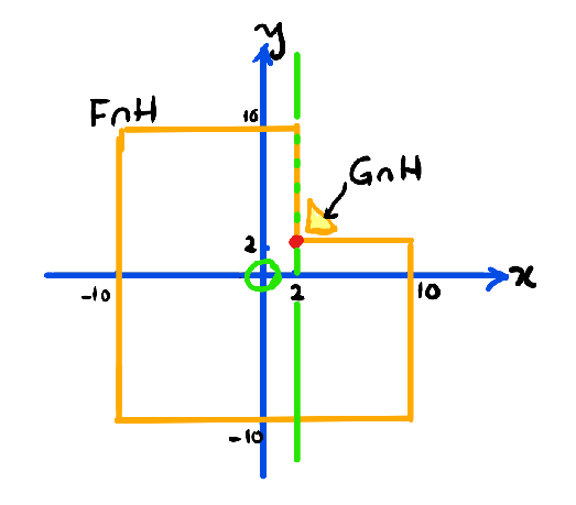
Figure 8: Counterexample.

Let $f_{0}$ be the boundary feature of $F$ that is closest to circle $C$. Clearly, $f_{0}$ is the vertical line $\langle x=2,y=2\rangle$. Moreover, $\mathrm{Sep}(C,f_{0})=2\sqrt{2}-1<1.82$. Now, slightly perturb $F$ so that $f_{0}$ is slightly non-vertical, but it’s projection onto the $(x,y)$-plane is the line $y=2$ (in Figure 8, $f_{0}$ is the red dot, and $y=2$ is the green line). We also verify that $\mathrm{Sep}^{\prime}(C,f_{0})=\sqrt{5}\simeq 2.36$.

It is also important to see that all the other boundary features $f\neq f_{0}$ of $F$, we have $\mathrm{Sep}^{\prime}(C,f)>2$. To see this, there are 2 possibilities for $f$: if $f$ is an edge, this is clear. If $f$ is a face, this is also clear unless the face is bounded by $f_{0}$ (there are two such faces). In this case, our algorithm sets $\mathrm{Sep}^{\prime}(C,f)$ to $\mathrm{Sep}^{\prime}(C,f_{0})$ which is $>2.23$. Note that $F$ does not have any corner features.

Now construct any convex polyhedron $G\subseteq{\mathbb{R}}^{3}$ that is disjoint from $F$ such that boundary feature of $G$ that is closest to $C$ is a corner $g_{0}=(2.1,2.1,0)$. It is easy to construct such a $G$. Moreover, we see that $\mathrm{Sep}(C,g_{0})=\mathrm{Sep}^{\prime}(C,g_{0})=\sqrt{2(2.1)^{2}}-1\simeq 1.97$.

Suppose $\Omega=F\cup G$ and the translational and rotational parts of $B$ are given by $B^{t}=[-1/2,1/2]^{2}$ and $B^{r}=[-1/8,1/8,1]$. We may assume that $\widetilde{\phi}(B)$ is empty. To classify $B$, we look at the set $\widetilde{\phi}(parent(B))$. Say the translational and rotational parts of $parent(B)$ are $[-1/2,3/2]^{2}$ and $[-1/8,3/8,1]$, respectively. In this case $\widetilde{\phi}(parent(B))$ contains any $g_{0}$ (and possibly $f_{0}$). In any case, $g_{0}$ would be regarded as the closest feature in $\widetilde{\phi}(parent(B))$ because we use $\mathrm{Sep}^{\prime}(C,f)$ for comparison. Based on $g_{0}$, our algorithm would decide that $B$ is $\mathtt{FREE}$ when in fact $B$ is $\mathtt{STUCK}$.

References

- [1] S. Basu, R. Pollack, and M.-F. Roy. Algorithms in Real Algebraic Geometry. Algorithms and Computation in Mathematics. Springer, 2nd edition, 2006.
- [2] H. Bennett, E. Papadopoulou, and C. Yap. Planar minimization diagrams via subdivision with applications to anisotropic Voronoi diagrams. Eurographics Symposium on Geometric Processing, 35(5), 2016. SGP 2016, Berlin, Germany. June 20-24, 2016.
- [3] R. A. Brooks and T. Lozano-Perez. A subdivision algorithm in configuration space for findpath with rotation. In Proc. 8th Intl. Joint Conf. on Artificial intelligence - Volume 2, pages 799–806, San Francisco, CA, USA, 1983. Morgan Kaufmann Publishers Inc.
- [4] J. Canny. Computing roadmaps of general semi-algebraic sets. The Computer Journal, 36(5):504–514, 1993.
- [5] H. Choset, K. M. Lynch, S. Hutchinson, G. Kantor, W. Burgard, L. E. Kavraki, and S. Thrun. Principles of Robot Motion: Theory, Algorithms, and Implementations. MIT Press, Boston, 2005.
- [6] H. Choset, B. Mirtich, and J. Burdick. Sensor based planning for a planar rod robot: Incremental construction of the planar Rod-HGVG. In IEEE Intl. Conf. on Robotics and Automation (ICRA’97), pages 3427–3434, 1997.
- [7] J. Cox and C. K. Yap. On-line motion planning: case of a planar rod. Annals of Mathematics and Artificial Intelligence, 3:1–20, 1991. Special journal issue. Also: NYU-Courant Institute, Robotics Lab., No.187, 1988.
- [8] J. Denny, K. Shi, and N. M. Amato. Lazy Toggle PRM: a Single Query approach to motion planning. In Proc. IEEE Int. Conf. Robot. Autom. (ICRA), pages 2407–2414, 2013. Karlsrube, Germany. May 2013.
- [9] D. Eberly. Distance to circles in 3D, May 31, 2015. Downloaded from https://www.geometrictools.com/Documentation/Documentation.html.
- [10] M. S. el Din and E. Schost. A baby steps/giant steps probabilistic algorithm for computing roadmaps in smooth bounded real hypersurface. Discrete and Comp. Geom., 45(1):181–220, 2011.
- [11] H. Everett, C. Gillot, D. Lazard, S. Lazard, and M. Pouget. The Voronoi diagram of three arbitrary lines in . In 25th European Workshop on Computational Geometry (EuroCG’09), 2009. March 2009, Bruxelles, Belgium.
- [12] H. Everett, D. Lazard, S. Lazard, and M. S. el Din. The Voronoi diagram of three lines. Discrete and Comp. Geom., 42(1):94–130, 2009. See also 23rd SoCG, 2007. pp.255–264.
- [13] D. Halperin, E. Fogel, and R. Wein. CGAL Arrangements and Their Applications. Springer-Verlag, Berlin and Heidelberg, 2012.
- [14] D. Halperin, O. Salzman, and M. Sharir. Algorithmic motion planning. In J. E. Goodman, J. O’Rourke, and C. Toth, editors, Handbook of Discrete and Computational Geometry, chapter 50. Chapman & Hall/CRC, Boca Raton, FL, 3rd edition, 2017. Expanded from second edition.
- [15] M. Hemmer, O. Setter, and D. Halperin. Constructing the exact Voronoi diagram of arbitrary lines in three-dimensional space — with fast point-location. In Proc. European Symposium on Algorithms (ESA 2010), volume 6346 of Lecture Notes in Computer Science, pages 398–409. Springer Berlin / Heidelberg, 2010.
- [16] V. Koltun. Pianos are not flat: rigid motion planning in three dimensions. In Proc. 16th ACM-SIAM Sympos. Discrete Algorithms, pages 505–514, 2005.
- [17] S. M. LaValle. Planning Algorithms. Cambridge University Press, Cambridge, 2006.
- [18] J. Y. Lee and H. Choset. Sensor-based planning for a rod-shaped robot in 3 dimensions: Piecewise retracts of . Int’l. J. Robotics Research, 24(5):343–383, 2005.
- [19] Z. Luo, Y.-J. Chiang, J.-M. Lien, and C. Yap. Resolution exact algorithms for link robots. In Proc. 11th Intl. Workshop on Algorithmic Foundations of Robotics (WAFR ’14), volume 107 of Springer Tracts in Advanced Robotics (STAR), pages 353–370, 2015. Aug. 3-5, 2014, Boǧazici University, Istanbul, Turkey.
- [20] J. R. Munkres. Topology. Prentice-Hall, Inc, second edition, 2000.
- [21] M. Nowakiewicz. MST-Based method for 6DOF rigid body motion planning in narrow passages. In Proc. IEEE/RSJ International Conf. on Intelligent Robots and Systems, pages 5380–5385, 2010. Oct 18–22, 2010. Taipei, Taiwan.
- [22] C. Ó’Dúnlaing, M. Sharir, and C. K. Yap. Retraction: a new approach to motion-planning. ACM Symp. Theory of Comput., 15:207–220, 1983.
- [23] C. Ó’Dúnlaing and C. K. Yap. A “retraction” method for planning the motion of a disc. J. Algorithms, 6:104–111, 1985. Also, Chapter 6 in Planning, Geometry, and Complexity, eds. Schwartz, Sharir and Hopcroft, Ablex Pub. Corp., Norwood, NJ. 1987.
- [24] J. T. Schwartz and M. Sharir. On the piano movers’ problem: I. the case of a two-dimensional rigid polygonal body moving amidst polygonal barriers. Communications on Pure and Applied Mathematics, 36:345–398, 1983.
- [25] J. T. Schwartz and M. Sharir. On the piano movers’ problem: II. General techniques for computing topological properties of real algebraic manifolds. Advances in Appl. Math., 4:298–351, 1983.
- [26] J. T. Schwartz and M. Sharir. On the piano movers’ problem: V. the case of a rod moving in three-dimensional space amidst polyhedral obstacles. Comm. Pure and Applied Math., 37(6):815–848, 1984.
- [27] M. Sharir, C. O’D’únlaing, and C. Yap. Generalized Voronoi diagrams for moving a ladder I: topological analysis. Communications in Pure and Applied Math., XXXIX:423–483, 1986. Also: NYU-Courant Institute, Robotics Lab., No. 32, Oct 1984.
- [28] M. Sharir, C. O’D’únlaing, and C. Yap. Generalized Voronoi diagrams for moving a ladder II: efficient computation of the diagram. Algorithmica, 2:27–59, 1987. Also: NYU-Courant Institute, Robotics Lab., No. 33, Oct 1984.
- [29] V. Sharma and C. K. Yap. Robust geometric computation. In J. E. Goodman, J. O’Rourke, and C. Tóth, editors, Handbook of Discrete and Computational Geometry, chapter 45, pages 1189–1224. Chapman & Hall/CRC, Boca Raton, FL, 3rd edition, 2017. Revised and expanded from 2004 version.
- [30] I. Şucan, M. Moll, and L. Kavraki. The Open Motion Planning Library. IEEE Robotics & Automation Magazine, 19(4):72–82, 2012. http://ompl.kavrakilab.org.
- [31] C. Wang, Y.-J. Chiang, and C. Yap. On soft predicates in subdivision motion planning. Comput. Geometry: Theory and Appl. (Special Issue for SoCG’13), 48(8):589–605, Sept. 2015.
- [32] C. Yap. Soft subdivision search in motion planning. In A. Aladren et al., editor, Proc. 1st Workshop on Robotics Challenge and Vision (RCV 2013), 2013. A Computing Community Consortium (CCC) Best Paper Award, Robotics Science and Systems Conf. (RSS 2013), Berlin. In arXiv:1402.3213.
- [33] C. Yap. Soft subdivision search and motion planning, II: Axiomatics. In Frontiers in Algorithmics, volume 9130 of Lecture Notes in Comp. Sci., pages 7–22. Springer, 2015. Plenary talk at 9th FAW. Guilin, China. Aug. 3-5, 2015.
- [34] C. Yap, Z. Luo, and C.-H. Hsu. Resolution-exact planner for thick non-crossing 2-link robots. In Proc. 12th Intl. Workshop on Algorithmic Foundations of Robotics (WAFR ’16), 2016. Dec. 13-16, 2016, San Francisco. The appendix in the full paper (and arXiv from http://cs.nyu.edu/exact/ (and arXiv:1704.05123 [cs.CG]) contains proofs and additional experimental data.
- [35] C. Yap, V. Sharma, and J.-M. Lien. Towards exact numerical Voronoi diagrams. In 9th Int’l Symp. of Voronoi Diagrams in Science and Engineering (ISVD)., pages 2–16. IEEE, 2012. Invited talk. June 27-29, 2012, Rutgers University, NJ.
- [36] C. K. Yap. Algorithmic motion planning. In J. Schwartz and C. Yap, editors, Advances in Robotics, Vol. 1: Algorithmic and geometric issues, volume 1, pages 95–143. Lawrence Erlbaum Associates, 1987.
- [37] L. Zhang, Y. J. Kim, and D. Manocha. Efficient cell labeling and path non-existence computation using C-obstacle query. Int’l. J. Robotics Research, 27(11–12):1246–1257, 2008.
- [38] B. Zhou, Y.-J. Chiang, and C. Yap. Soft subdivision motion planning for complex planar robots. In Proc. 26th European Symposium on Algorithms (ESA 2018), pages 73:1–73:14, 2018. Helsinki, Finland, Aug. 20-24, 2018.
- [39] D. Zhu and J.-C. Latombe. New heuristic algorithms for efficient hierarchical path planning. IEEE Transactions on Robotics and Automation, 7:9–20, 1991.