A constrained ICA-EMD Model for Group Level fMRI Analysis

Abstract

Independent component analysis (ICA), as a data driven method, has shown to be a powerful tool for functional magnetic resonance imaging (fMRI) data analysis. One drawback of this multivariate approach is, that it is not compatible to the analysis of group data in general. Therefore various techniques have been proposed in order to overcome this limitation of ICA. In this paper a novel ICA-based work-flow for extracting resting state networks from fMRI group studies is proposed. An empirical mode decomposition (EMD) is used to generate reference signals in a data driven manner, which can be incorporated into a constrained version of ICA (cICA), what helps to eliminate the inherent ambiguities of ICA. The results of the proposed workflow are then compared to those obtained by a widely used group ICA approach for fMRI analysis. In this paper it is demonstrated that intrinsic modes, extracted by EMD, are suitable to serve as references for cICA to obtain typical resting state patterns, which are consistent over subjects. By introducing these reference signals into the ICA, our processing pipeline makes it transparent for the user, how comparable activity patterns across subjects emerge. This additionally allows adapting the trade-off between enforcing similarity across subjects and preserving individual subject features.

1 Introduction

Independent component analysis (ICA) is a data driven tool, which is widely employed for functional magnetic resonance imaging (fMRI) data analysis. Based on a linear mixture model, either spatially (McKeown et al., 1998) or temporally (Biswal and Ulmer, 1999) independent components (ICs) can be obtained with ICA, without the requirement of prior information in form of anatomical regions of interest or temporal activation profiles. One problem of ICA is that, because of inherent indeterminacies, it is in general not suitable for group studies. Different subjects have different time courses and spatial maps, and the extracted components will be sorted differently. This can make it difficult to find comparable activation patterns between subjects and draw inferences from subject groups. So far various approaches have been proposed in order to overcome these shortcomings of ICA (Calhoun et al., 2009). Combining components obtained by single subject ICA-based on spatial correlation or clustering was proposed by Calhoun et al. (2001a) and Esposito et al. (2005). Another possibility is the spatial or temporal concatenation of the individual datasets to obtain components in a single ICA step from a group dataset and the employment of back-reconstruction approaches to obtain subject specific components (Svensén et al., 2002; Calhoun et al., 2001b). These concatenation-based approaches were compared with a simple across-subject averaging by Schmithorst and Holland (2004). A more involved approach considered a tensorial extension of ICA, presented by Beckmann and Smith (2005). The authors extended the probabilistic ICA (PICA) model by adding a third dimension representing subject-related dependencies in addition to the spatio-temporal dimensions. The model represents a three-way factor analysis similar to the well-known PARAFAC model (Harshman and Lundy, 1994).

A popular paradigm used to generate data for applying the above mentioned exploratory matrix factorization techniques is the so-called resting-state. During this paradigm, subjects either rest with eyes open fixating a fixation cross, or with eyes closed. Usually, subjects are instructed not to fall asleep and to let their mind wander. Contrary to the simplicity of the paradigm, the generated database has complex spatial structure and temporal dynamics, which arise from low-frequency fluctuations in the BOLD signal (Fox and Raichle, 2007). Furthermore the data is characterized by large spatial dimension and the lack of triggers or any underlying paradigm, which are usually used in task-based fMRI investigations. Because of the latter two aspects, exploratory matrix factorization techniques are appropriate to handle the large amount of data and explore the complex spatial and temporal structure. In this context, ICA-based pipelines have emerged as a state-of-the-art approach to investigate rs-fMRI data (Allen et al., 2011; Remes et al., 2011). This decomposition of resting-state fMRI data results in a so-called parcellation of the cortex into brain networks composed of functionally similar brain areas. In the literature, common brain networks are default-mode, cognitive control, visual, somatomotor, sub-cortical, auditory, cerebellar, depending on the function of the brain areas included in each network (Allen et al., 2014).

In this paper, a hybrid method is proposed for extracting resting state networks (RSNs) from fMRI data, based on constrained ICA (cICA) and empirical mode decomposition (EMD). This constrained extension of ICA optimizes besides the statistical independence, the similarity to a given reference signal. Incorporating a reference into ICA, in the framework of an augmented Lagrangian approach, helps to obtain more robust ICs and can eliminate the ambiguities of ICA (Lu and Rajapakse, 2006; Lin et al., 2009; Rodriguez et al., 2014). In this paper, like (Lin et al., 2009), spatial reference maps were employed to extract resting state networks from fMRI data. It is shown that an EMD based image decomposition technique, denoted as Green’s function in tension based bi-dimensional ensemble EMD (GiT-BEEMD) (Al-Baddai et al., 2016b), produces suitable references for cICA. This two-dimensional extension of EMD allows to decompose images into so called bi-dimensional intrinsic mode functions (BIMFs) and can also be used to decompose volumetric fMRI images slice-wise. Because of its inherent natural ordering of the extracted intrinsic modes according to their spatial frequencies, EMD can easily generate prototype spatial maps. Similar spatial maps obtained with the EMD for each subject can be identified and averaged across subjects. In a next step these prototype spatial maps can serve as reference signals for a constrained ICA applied in parallel to the entire group of subjects. In this workflow the references are obtained from the same dataset as used for the analysis, so no prior information is required. A resting state fMRI dataset from the Human Connectome Project (Essen et al., 2012) is used to compare the results to those obtained by the widely used group ICA (gICA) based on temporal concatenation (Calhoun et al., 2001b). Finally potential benefits of the proposed approach are emphasized, by showing that this approach allows the user to actively shape the extracted resting state networks. The trade-off between enforcing a certain similarity across subjects and preserving individual subject features can be determined, and can be well adapted to optimally fulfill the requirements of different studies.

2 Material and Methods

The following subsections introduce the dataset employed, and describe the data analysis techniques, which combine cICA and GiT-BEEMD, as well as the processing steps of the gICA approach used for comparison. Also a flowchart of the proposed signal processing chain is provided.

2.1 Dataset

For this study a data set from the Human Connectome Project was employed (Essen et al., 2012). The S1200 release includes data from subjects which participated in four resting state fMRI sessions, lasting 14.4 minutes each and resulting in 1200 volumes per session. Customized Siemens Connectome Skyra magnetic resonance imaging (MRI) scanners at Washington University with a field strength of $\bf{B}_{0}=3\ Tesla$ were employed for data acquisition, using a multi-band (factor 8) technique (Moeller et al., 2010; Feinberg et al., 2010; Setsompop et al., 2012; Xu et al., 2012). The data was collected by gradient-echo echo-planar imaging (EPI) sequences with a repetition time $TR=720\ ms$ and an echo time $TE=31.1\ ms$, using a flip angle of $\theta=52^{\circ}$. The field of view was $FOV=208\ mm\times 180\ mm$ and $N_{s}=72$ slices with a thickness of $d_{s}=2\ mm$ were obtained, containing voxels with a size of $2\ mm\times 2\ mm\times 2\ mm$. The preprocessed version, including motion-correction, structural preprocessing and ICA-FIX denoising was chosen (Glasser et al., 2013; Jenkinson et al., 2002, 2012; Fischl, 2012; Smith et al., 2013; Salimi-Khorshidi et al., 2014; Griffanti et al., 2014). For the comparison of the two approaches, $10$ sessions from $10$ different subjects were selected from the database. A Gaussian smoothing with a half width $FWHM=5\ mm$ was then applied, using the SPM12 software package , and the first five images were discarded to account for magnetic saturation effects.

2.2 A hybrid cICA - EMD approach

In this section a new approach to deal with an ICA analysis across a group of subjects will be described. The flowchart in Figure 1 presents an overview of the various steps of the data analysis. All processing steps were performed in MATLAB 9.3 Release 2017b.

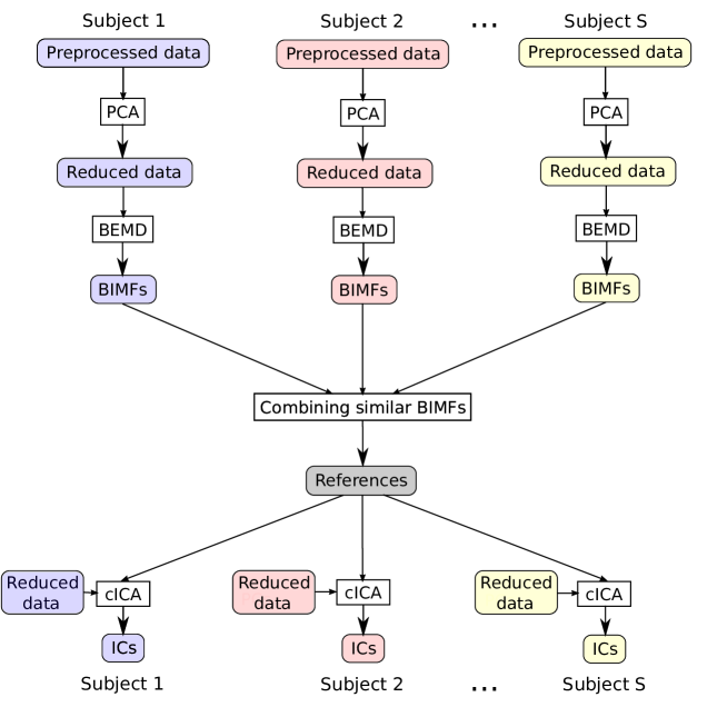
Figure 1: The flowchart sketches the main steps of the presented approach: First reducing the data with PCA, then extracting BIMFs with BEMD from the reduced data. Further these BIMFs of each subject are combined in order to get shared references for cICA, which finally help to obtain comparable ICs across subjects.

2.2.1 Preprocessing

The data as obtained from the data repository will be further pre-processed as explained in the following.

• In a first step, the voxel time series were linearly detrended and the voxel values were transformed to have zero mean and unit variance.

• Next a mask common to all subjects was used to exclude voxels that were located outside of the brain. The mask was created, employing the GIFT toolbox , using the ”Generate mask” option.

• The data of subject $s$ is stored in a $K\times L$-dimensional matrix $\mathbf{X}^{(s)}$, containing in its columns $\mathbf{x}_{l}(k)$ the temporal evolution of $L$ brain voxels at $K$ time points.

• Then principal component analysis (PCA) related dimension reduction is performed, based on the singular value decomposition (SVD) of $\mathbf{X}^{(s)}=\mathbf{U}^{(s)}\boldsymbol{\Sigma}^{(s)}\mathbf{V}^{(s)T}$. If the row mean of $\mathbf{X}^{(s)}$ is removed, then $\textbf{U}^{(s)}$ contains the eigenvectors of the covariance matrix $\textbf{C}^{(s)}\propto\textbf{X}^{(s)}\textbf{X}^{(s)T}$ in its columns. The eigenvectors with largest eigenvalues indicate the directions of largest variance, which are denoted as principal components (PCs) (Jolliffe, 2014).

• Next, the fMRI images of each subject were projected onto the first $M=20$ PCs $\mathbf{X}_{M}^{(s)}=(\mathbf{U}_{M}^{(s)})^{T}\,\mathbf{X}^{(s)}$. This reduces the number of images per session to $M=20<K$.

• Finally, from the reduced data sets the image slices were reconstructed to enter into the GiT-BEEMD analysis, while the reduced data $\mathbf{X}_{M}^{(s)}$ entered directly into the cICA processing path. The number of selected principal components $M$ determines the number of sources, estimated in the cICA step. A relatively low order of $M=20$ was chosen, to obtain robustly observed, large-scale resting state networks (van den Heuvel and Pol, 2010), and to make it easy to identify extracted networks, which are suitable for comparison of results in section 3.

2.2.2 Green’s function-based ensemble empirical mode decomposition

For the next step, the extraction of suitable reference signals for cICA, the GiT-BEEMD technique was employed (Al-Baddai et al., 2016b). The idea of this technique is to decompose a two-dimensional brain slice $I(\mathbf{r})=I(x,y)$ into bi-dimensional intrinsic mode functions (BIMFs):

$$I(x,y)=\sum_{j=1}^{J}b_{j}(x,y)$$ (1)

Here $b_{j}(x,y)$ denotes the $j$-th BIMF, which is estimated iteratively as described in Appendix A.1, and, in our notation, we include the residuum $r(x,y)$ as intrinsic mode $b_{J}(x,y)$. The first extracted BIMF contains the highest spatial frequency, which will decrease in every additionally extracted BIMF (Al-Baddai et al., 2016b).

Each brain slice was decomposed into five intrinsic modes and one residuum by repeating the sifting step five times. The ensemble step was repeated only twice, whereby noise was either added or subtracted from the data once at each step. The assisting noise was generated with a noise amplitude of $a_{\eta}=0.2$. The tension parameter was initialized to $T_{1}=0.9$ and reduced after the extraction of the $j$-th BIMF $b_{j}$ to $T_{j+1}=T_{j}-\frac{1}{J}$. This avoids blob-like artifacts in low frequency modes, if the tension parameter is set too high (Al-Baddai et al., 2016b). An example of a decomposition is provided in figure 2. BIMFs with high spatial frequencies show highly localized spatial activation patterns which are spread all over the brain slice, while BIMFs with lower spatial frequencies concentrate the activity in specific areas in the brain. A combination of lowest spatial frequency intrinsic mode plus the residuum, i. e. $b_{5}(x,y)+b_{6}(x,y)\equiv b_{56}(x,y)$, proved most appropriate to be used as a reference mode for cICA. From all decomposed two-dimensional slices, the corresponding modes $b_{56}(x,y)$ were organized into a three-dimensional data array, which then was concatenated into a 3D volume intrinsic mode function (VIMF). Decomposing the $M=20$ brain volumes per subject in PC subspace results in $M$ VIMFs per subject. For the next processing steps the voxels inside of the brain are sorted into an $M\times L$ matrix again, denoted as $\mathbf{V}_{M}^{(s)}$.

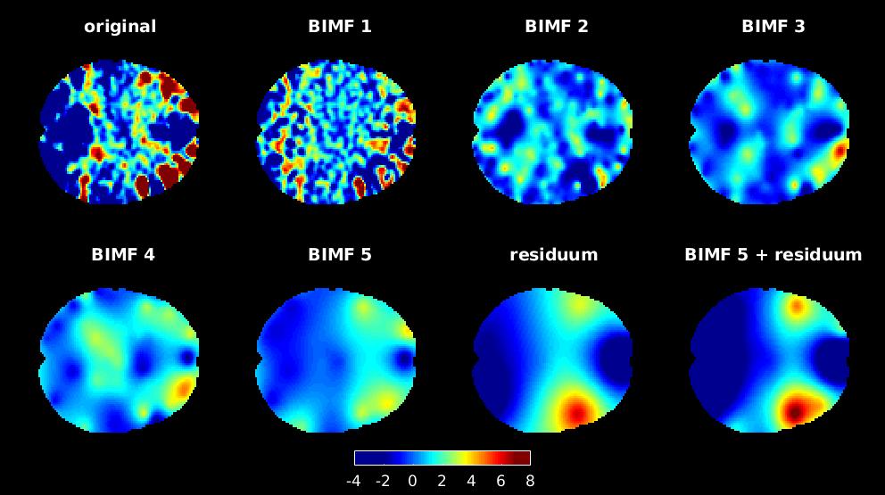
Figure 2: Example of a decomposition of a slice with GiT-BEEMD into 5 BIMFs and a residuum. Also the combination of fifth BIMF and residuum is illustrated. A mask was applied after the decomposition to set all intensity values that were located outside of the scanned brain to zero.

In order to extract from each subject RSNs, which are consistent across the proband cohort, corresponding intrinsic modes need to be identified. Averaging most similar modes between subjects then yields proper common reference signals for all subjects to be employed in a cICA of fMRI datasets. A visual inspection of the VIMFs of any two randomly chosen subjects showed that corresponding spatial patterns might occur in different rows of $\mathbf{V}_{M}^{(s)}$. Hence first the extracted VIMFs need to be ordered according to their similarity between subjects. An efficient way to assign similar VIMFs between subjects is offered by the assignment algorithm proposed by Munkres (1957), based on the Hungarian method developed by Kuhn (1955). After computing the proper correspondences between the VIMFs of all subjects, the references $\mathbf{R}$, to be used in the cICA algorithm, then are obtained by averaging the corresponding VIMFs across all subjects.

To summarize, the reference signals are computed as follows:

1. Initialize the reference as $\mathbf{R}=\mathbf{V}_{M}^{(1)}$

2. For $s=2,\ldots,S$, do:

   1. Apply the Hungarian algorithm and re-order the rows of $\mathbf{V}_{M}^{(s)}\rightarrow\tilde{\mathbf{V}}_{M}^{(s)}$

   2. Update the reference $\mathbf{R}\leftarrow\frac{s-1}{s}\mathbf{R}+\frac{1}{s}\tilde{\mathbf{V}}_{M}^{(s)}$

To apply the Hungarian algorithm, a cost function $1-\rho(\mathbf{R},\mathbf{V}_{M}^{(s)})$ is defined, which, if optimized, results in an ordering of the rows in $\mathbf{V}_{M}^{(s)}$ such that the sum of the correlation coefficients between pairs of rows in the two matrices is maximized. Note that the algorithm achieves the re-ordering without calculating all $M!$ possible assignments. Finally, each row of $\mathbf{R}$ is normalized, having entries with zero mean and unit variance, and $M=20$ references for cICA algorithm are obtained.

2.2.3 Constrained ICA

Sources $\mathbf{Y}_{M}=[\mathbf{y}_{1},\ldots,\mathbf{y}_{L}],\mathbf{y}\in\mathbb{R}^{M}$ can be blindly estimated from the mixtures $\mathbf{X}_{M}=[\mathbf{x}_{1},\ldots,\mathbf{x}_{L}],\mathbf{x}\in\mathbb{R}^{M}$ according to:

$$\mathbf{Y}_{M}=\mathbf{W}\mathbf{X}_{M}$$ (2)

with the demixing matrix defined as $\mathbf{W}=[\mathbf{w}_{1},\ldots,\mathbf{w}_{M}]^{T}$, where $\mathbf{w}^{T}_{m}$ are the rows of the demixing matrix and $\mathbf{X}_{M}$ collects all $L$ samples of the projected data after being spatially transformed to zero mean and unit variance.

Finding a demixing matrix is solved by designing an optimization problem where inequality and equality constraints are integrated in an augmented Lagrangian formulation. The inequality constraint terms in the Lagrange function are re-written as equality constraints with the help of a slack variable (Lu and Rajapakse, 2006). After finding the optimal value of these slack variables, the modified version of the augmented Lagrangian function is written as

$$\mathcal{L}(\mathbf{W},\boldsymbol{\mu}) = J(\mathbf{W})+\sum_{m=1}^{M}\frac{1}{2\gamma_{m}}\left[(\max\{0,\gamma_{m}h_{m}(\mathbf{w}^{T}_{m})+\mu_{m}\})^{2}-\mu_{m}^{2}\right]$$ (3)

where the $\mu_{m}$ are the Lagrangian parameters, while $\gamma_{m}$ represents a user defined penalty. The first term $J(\mathbf{W})$ reflects the cost function of ICA and the second term in the Lagrangian is related with the inequality constraint, which compares the $m$-th extracted component with the corresponding reference signal:

$$h(\mathbf{w}^{T}_{m})=\varsigma_{m}-\epsilon(\mathbf{w}^{T}_{m}\mathbf{x},r_{m})\leq 0$$ (4)

where $\epsilon(\cdot)$ is a similarity measure and $\varsigma_{m}$ is a threshold parameter. Similarity is conventionally expressed either through a correlation measure $\mathbb{E}\{y_{m}r_{m}\}$ or the mean squared error $\mathbb{E}\{(y_{m}-r_{m})^{2}\}$, with $y_{m}=\mathbf{w}_{m}^{T}\mathbf{x}$. The expected value is approximated by an average over the available data.

Estimating the demixing matrix $\mathbf{W}$, given the constraint introduced above, can be achieved in different ways, based either on negentropy-like costs functions (points 1 - 3) or on a maximum likelihood estimate (point 4):

1. Simply one IC, most similar to the given reference signal, can be extracted. This approach can easily be extended to a multi-reference cICA. However, this additionally requires a decorrelation of the weights during each iteration to prevent different weights from converging to identical estimations (Lu and Rajapakse, 2006).

2. Lu and Rajapakse (2006) introduced an objective function for cICA,which contained an additional equality constraint to bound the weights. Later, a simplification was introduced by Lin et al. (2007), where equality constraints were omitted, rather the weight vectors were normalized at each iteration instead.

3. Also cICA based on fixpoint learning (Lin et al., 2009) was proposed, which should overcome the limitations of the second order Newton-like learning used in the cICA algorithm of Lu and Rajapakse (2006).

4. Finally, yet another version, using a cost function $J(\mathbf{W})$ based on a maximum likelihood estimate, has been proposed (Rodriguez et al., 2014) according to

   $$J(\mathbf{W})\approx\mathbb{E}\left\{\sum\limits_{m=1}^{M}\log(p(\mathbf{w}_{m}^{T}\mathbf{x}))\right\}+\log|\det(\mathbf{W})|$$ (5)

   An iterative procedure is then derived to update the parameters $\boldsymbol{\mu}=[\mu_{1},\ldots,\mu_{M}]^{T}$ and the de-mixing matrix $\mathbf{W}$. Thereby a decoupling scheme based on a Gram - Schmidt orthogonalization is proposed, finally yielding the following objective function

   $$J(\mathbf{w}_{m})\propto\mathbb{E}\left\{\log(p(\mathbf{w}_{m}^{T}\mathbf{x}))\right\}+\log|\mathbf{d}_{m}^{T}\mathbf{w}_{m}|$$ (6)

   where the decoupling vector $\mathbf{d}_{m}\in\mathbb{R}^{M\times 1}$ is defined through $\tilde{\mathbf{W}}_{m}\mathbf{d}_{m}=0$ and where $\tilde{\mathbf{W}}_{m}\in\mathbb{R}^{(M-1)\times M}$ denotes the de-mixing matrix without entries to the $m$-th row.

It has been shown by Cardoso (1997) that a maximum likelihood approach to ICA is equivalent to the seminal Infomax approach put forward by Bell and Sejnowski (1995). Thus, in analogy to the maximum likelihood approach, a constrained and decoupled version of the extended Infomax algorithm can be obtained (Rodriguez et al., 2014). The extended Infomax algorithm is often used in an analysis of fMRI data (Correa et al., 2007) and was also used in this study as the basis of the cICA. A more detailed description of this algorithm and a proper metacode are given in Appendix A.2 for the convenience of the reader.

The data, projected onto the first $M=20$ PCs, and the $M$ references, transformed to zero mean and unit variance, together enter the cICA algorithm to finally extract $M=20$ ICs. The weights are initialized with small random values, and the learning rate for the weights is set to $\eta=0.5$. The scalar penalty can be set to 3 (Rodriguez et al., 2014). The influence of the references can be well determined by adjusting the threshold parameter. Therefore different settings have been studied, using the correlations $\mathbb{E}\{y_{m}r_{m}\}$ as distance measures, and results are presented in section 3.

2.3 Group-ICA

Generally fMRI data is compared across a group of subjects by employing the gICA algorithm put forward by Calhoun and his group (Calhoun et al., 2001a). This gICA is made available in the GIFT toolbox and was incorporated in the study for comparison. Voxel time series were preprocessed by variance normalization through linear detrending and transforming the data to zero mean and unit variance. The single subject data matrices $\textbf{X}^{(s)}_{K\times L}$ enter the first PCA step, with the temporal evolution of $L$ brain voxels at $K$ time points in columns. The subject datasets then were projected onto the first $M^{\prime}=1.5\cdot M=30$ PCs in this step by applying an SVD to the data matrix. Then the $S$ reduced $M^{\prime}\times L$ matrices $\mathbf{X}_{M^{\prime}}^{(s)}$ on subject level were concatenated to an $(S\cdot M^{\prime})\times L$ group matrix $\textbf{X}_{S\cdot M^{\prime}}^{(g)}$ entering a second PCA step. The group matrix is projected onto $M=20$ PCs, resulting in a reduced $M\times L$ matrix $\mathbf{X}_{M}^{(g)}$. The spatial maps $\mathbf{S}_{M}$ are extracted from $\mathbf{X}_{M}^{(g)}=\mathbf{A}\mathbf{S}_{M}$ by the extended Infomax algorithm (Lee et al., 1999) and by additionally employing the ICASSO option (Himberg et al., 2004), running the ICA algorithm ten times with different initializations to assure greater stability. Subject specific spatial $\mathbf{S}_{M}^{(s)}$ maps were obtained by the GICA3 (Erhardt et al., 2011) back-reconstruction approach. From these maps $M$ mean networks $\langle\mathbf{S}_{m*}\rangle,\;m=1,\ldots,M$ were obtained by averaging $\mathbf{S}_{M}^{(s)}$ over the subjects, i. e. $\langle\mathbf{S}_{M}\rangle=\frac{1}{S}\sum_{s=1}^{S}\mathbf{S}_{M}^{(s)}$.

3 Results

The goal of the study was to compare RSNs obtained with the newly proposed cICA-EMD approach as opposed to RSNs resulting from the conventional gICA approach. RSNs denote functionally connected brain areas which, however, are anatomically separated but maintain a high level of activity in a resting state of the proband. They are represented in this study by the ICs extracted with the discussed techniques. In this study $M=20$ ICs were extracted with either method. Comparable RSNs, obtained by the different approaches, were identified by visual inspection and are depicted in figure 3. There, references used for cICA are shown in the first row, while in the second row the ICs obtained therewith are presented, computed as mean ICs over subjects. In the third row of figure 3 the mean ICs obtained by gICA are exhibited. The significance of the resulting ICs was tested with a one sample student’s T-test by employing the SPM12 software package . The resulting spatial maps of t-values are depicted in the fourth and fifth row in figure 3. Spatial maps were thresholded at a significance level of $p<0.001$ $(t=4.30,df=9)$.

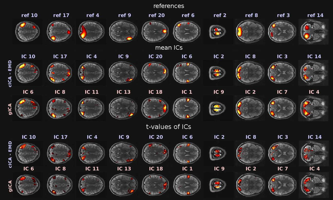
Figure 3: This figure illustrates RSNs, which were obtained by the two different approaches. The first row shows the references used for cICA, while the second row exhibits mean ICs, averaged over the subject cohort and computed with the newly proposed cICA-EMD method. These ICs are contrasted in the third row with mean ICs obtained by gICA. In the fourth and fifth row of this figure, t-values of the RSNs can be found. All depicted slices were chosen such that they intersect the peak activation voxel of the corresponding ICs obtained by gICA. For visualization purposes, the activations of the networks shown in the first three rows are normalized to zero mean and unit variance. Furthermore, in accordance with common usage, the voxel intensities $\hat{I}(\mathbf{r})$ were thresholded by $\hat{I}(\mathbf{r})>2$, and in the sixth and ninth column the threshold was adjusted to $\hat{I}(\mathbf{r})>1.5$ for better recognizability of the networks. The color range of the heatmap was adjusted to the largest intensity value in every pictured slice.

Most prominent brain areas are in IC 10/6 (obtained by cICA-EMD/gICA) the left inferior parietal lobule, in IC 17/8 the right angular/supramarginal gyrus, in IC 4/11 the superior occipital gyrus, in IC 9/13 the right inferior frontal gyrus, in IC 20/18 the anterior cingulate cortex, in IC 6/1 the precentral gyrus, in IC 2/9 the paracentral lobule, in IC 8/2 the middle occipital gyrus and in IC 3/7 the middle temporal gyrus. The obtained independent networks, representing well observed RSNs (van den Heuvel and Pol, 2010), and can be further grouped based on to their functions. The corresponding attentional and default mode networks are depicted in the first five columns, while the extracted auditory and sensorimotor networks are shown in the sixth and seventh column. Next, in the eighth and ninth column, visual networks are represented, and in the last column the cerebellum is shown. The similarity threshold for cICA was set to $\varsigma=0.5$ in this example. All resting state networks obtained with both approaches, including the employed references are provided in the supplement.

The motivation of different group ICA approaches is to make this explorative analysis technique suitable for studies, where it is necessary to compare extracted networks between different subjects. This means issues with permutation indeterminacy and reproducibility of ICA have to be overcome, to obtain well comparable networks. Therefore a measure of interest for the evaluation of the two different approaches could be the consistency of activation patterns across subjects. This consistency was quantified by measuring how strong a resting state network $(\mathbf{y}^{(s)})_{m}^{T}\in\mathbb{R}^{L}$ from one subject $s$ differs on average from the mean network $\langle\mathbf{y}\rangle^{T}_{m}=\frac{1}{S}\sum_{s=1}^{S}(\mathbf{y}^{(s)})_{m}^{T}$ across subjects. Pearson’s correlation $\rho\big{(}(\mathbf{y}^{(s)})_{m}^{T},\langle\mathbf{y}\rangle_{m}\big{)}$ was used to measure the correlation between standardized subject networks $\mathbf{y}_{m}^{(s)}$ and the related mean networks $\langle\mathbf{y}\rangle^{T}_{m}$. The following consistency measure is used:

$$K_{per}(\mathbf{y}_{m})=\frac{1}{S}\sum_{s=1}^{S}\rho\big{(}(\mathbf{y}^{(s)})_{m}^{T},\langle\mathbf{y}\rangle_{m}\big{)}$$ (7)

This consistency measure was evaluated for all ICs obtained with the cICA-EMD approach for different settings of the similarity threshold $\varsigma$. An equivalent procedure was followed using the results from applying the gICA algorithm. The results are listed in table 1.

Table 1: Consistency values of ICs obtained by the proposed cICA-EMD approach for different settings of the similarity threshold $\varsigma$, as well as the values of ICs obtained by gICA. ICs were sorted like in figure 3, so each column shows consistency values of comparable extracted networks.

cICA-EMD
threshold00 IC # 10 17 40 90 20 60 20 8 30 140 0.40 0.62 0.58 0.63 0.59 0.55 0.56 0.60 0.54 0.60 0.53 0.50 0.67 0.68 0.68 0.68 0.66 0.66 0.69 0.65 0.70 0.59 0.60 0.71 0.76 0.73 0.74 0.71 0.72 0.71 0.73 0.73 0.62


gICA
IC # 60 80 11 13 18 10 90 20 70 40 0.73 0.65 0.68 0.70 0.66 0.66 0.66 0.70 0.71 0.60

By adjusting the threshold parameter $\varsigma$, it is possible to well determine the influence of the constraint during the optimization, so choosing a smaller threshold allows for more variability in the estimated components across subjects. Increasing the threshold increases the similarity between subject specific components and common references. This means that if the similarity between every subject component and the shared reference increases, also the similarity of components across subjects will increase, what is quantified by the consistency measure in equation 7. Figure 4 illustrates the behavior of the consistency in dependence of the similarity threshold $\varsigma$ in comparison to gICA. If the threshold parameter is set to a value of $\varsigma=0.40$, the consistency is lower in comparison to gICA. By further increasing this threshold to a value of $\varsigma=0.60$ the consistency of estimated resting state networks with the proposed approach exceeds that of gICA.

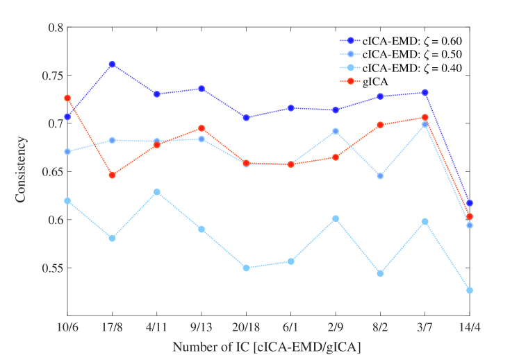
Figure 4: The figure illustrates the consistency values of the respective ICs. The numbers on the x-axis refer to the IC number of the cICA-EMD versus the gICA approach.

4 Discussion

The motivation of this paper was to propose a novel workflow for extracting resting state networks consistent across a group of subjects. At first the dimensionality of the fMRI dataset was reduced at subject level with PCA. From that data intrinsic modes were extracted by employing the GiT-BEEMD algorithm (Al-Baddai et al., 2016b). These subject-specific intrinsic modes reflect spatial activity patterns at different spatial frequencies. Hence, for each underlying spatial frequency a common reference mode can be formed. It turned out that low frequency modes concentrate the activity into spatially contiguous patterns and were especially well suited to serve as reference modes for the extraction of independent components with a cICA algorithm. Note that if intrinsic spatial modes, which are naturally ordered according to their dominant local spatial frequency, are chosen as reference signals within a cICA, the resulting independent modes are also ordered in correspondence to their assigned intrinsic modes. Thus, the natural ordering of the intrinsic modes with respect to their spatial frequencies helps to overcome the permutation ambiguity of ICA in extracting consistent resting state networks across subjects. It was demonstrated that our fMRI data processing pipeline produces commonly observed resting state patterns. These functional networks were then compared to those obtained by the widely used gICA, based on a temporal concatenation of individual datasets (Calhoun et al., 2001b). It was shown that with the constrained extended Infomax algorithm (Rodriguez et al., 2014), the influence of the references upon the estimation of the related ICs could be well controlled. Based on the mathematically well described augmented Lagrangian framework in our workflow, it is transparent to the user with respect to how homologous resting state networks across subjects are deduced. In the presented processing pipeline, the cICA-EMD approach also allowed to shape the optimization procedure by adjusting the threshold parameter, which determines the impact of the reference onto the IC extraction. Choosing a lower threshold, e.g. allowing for a lower similarity to the references, more freedom could be given to the exploratory character of ICA and the formation of subject specific features. Defining a high threshold resulted, across subjects, in a higher consistency of the extracted resting state networks. These RSNs were even more consistent than those obtained by the conventional gICA. Although there is no exact ground truth on how resting state networks should ideally look like, the threshold can be chosen in a way such that the obtained networks optimally fulfill the requirements of a particular study. For example, when performing a classification task, the threshold can be chosen to maximize the accuracy of the classifier. So the good interpretability and high flexibility of the proposed processing pipeline can offer beneficial properties for applications in resting state studies.

Conflict of Interest Statement

The authors declare that the research was conducted in the absence of any commercial or financial relationship that could be construed as a potential conflict of interest.

Appendix A Appendix

A.1 A Green’s function-based bi-dimensional empirical mode decomposition

The process of extracting BIMFs $b_{j}(x,y)$ with a bi-dimensional EMD (BEMD) algorithm can be summarized in the following steps (Al-Baddai et al., 2016a; Nunes et al., 2003):

 

Bi-dimensional empirical mode decomposition

 

1. Choose the number of intrinsic modes $J$ and the number of sifting steps $N$ and set $r(x,y)=f(x,y)$

2. Extract the $j$-th BIMF by repeating the sifting steps $N$ times:

   1. Identify all local maxima and minima of the array $r(x,y)$

   2. Interpolate these local maxima to an upper envelope surface $s_{max}(x,y)$ and local minima to a lower envelope surface $s_{min}(x,y)$ and calculate the mean between upper envelope surface and lower envelope surface $s_{mean}(x,y)=0.5\,(s_{max}(x,y)+s_{min}(x,y))$

   3. Update $r(x,y)$ with $r(x,y)\leftarrow r(x,y)-s_{mean}(x,y)$

   4. If loop is finished, set $b_{j}(x,y)=r(x,y)$, otherwise repeat steps (a) - (d)

3. Subtract all calculated BIMFs $b_{1...j}$ from $f(x,y)$ to obtain new $r(x,y)=f(x,y)-\sum_{j<j+1}b_{j}(x,y)$

4. If all $J$ BIMFs are extracted, $r(x,y)$ is the residuum, otherwise repeat step 2 to compute the next BIMF $b_{j+1}$

 

Interpolation schemes, which are used to describe the upper and lower envelope surface, usually suffer from problems like computational load, boundary artefacts and over- and undershooting (Al-Baddai et al., 2016b). Using a Green’s function-based interpolation scheme, local maxima or minima can be considered as the known points of the envelope surface, which can be found with an 8-connected neighborhood strategy. Then surface envelopes $s(\textbf{r}_{u})$, at Cartesian coordinates $\textbf{r}_{u}=[x_{u},y_{u}]^{T}$, are represented as a weighted sum of Green’s functions (Wessel and Bercovici, 1998):

$$s(\textbf{r}_{u})=\sum_{n=1}^{N}v_{n}\Phi(\textbf{r}_{u},\textbf{r}_{n}),$$ (8)

where $\Phi(\textbf{r}_{u},\textbf{r}_{n})$ represent the Green’s functions and $v_{n}$ the corresponding weights. Further $\textbf{r}_{u}$ denotes a point where the surface is unknown and $\textbf{r}_{n}$ describes the $n$-th constraint, which corresponds to a local extremum. The Green’s function, expressed in 2D-Cartesian coordinates, reads as:

$$\Phi(\textbf{r}_{u},\textbf{r}_{n})=\mbox{log}(p|\textbf{r}_{u}-\textbf{r}_{n}|)+K_{0}(p|\textbf{r}_{u}-\textbf{r}_{n}|)$$ (9)

with $K_{0}(\cdot)$ representing the modified Bessel function of the second kind and zero order and $|\cdot|$ the Euclidean distance. Here $p^{2}=\frac{T}{D}$ is related with tension $T$ at the boundaries, and $D$ describes the flexural rigidity of the surface (Wessel and Bercovici, 1998). The estimation of the envelope surface is based on two steps. In a first step weights $v_{n}$ can be estimated by taking the known values of local maxima (or minima) as the values $s(\textbf{r}_{n})=[s(\textbf{r}_{1}),\,.\,.\,.\,,s(\textbf{r}_{N})]^{T}$ in a total of $N$ locations $\textbf{r}_{n}$ and solving a linear system of $N$ equations, described by equation 8. In a second step, if the weights $v_{n}$ are now obtained, the surface can be estimated at any point $\textbf{r}_{u}$.

To avoid mode mixing and boundary artifacts, a noise assisted ensemble version of the Green’s function based BEMD (GiT-BEEMD) can be used (Al-Baddai et al., 2016a). Adding and subtracting noise $\eta$ from the original image $f(x,y)$ leads to two noisy versions $\tilde{f}(x,y)^{*}:\tilde{f}^{+}(x,y)=f(x,y)+\eta$ and $\tilde{f}^{-}(x,y)=f(x,y)-\eta$. Both versions $\tilde{f}(x,y)^{*}$ can now be decomposed into BIMFs. By computing the mean as $0.5\,(\tilde{f}^{+}(x,y)+\tilde{f}^{-}(x,y))$ the original array $f(x,y)$ could be reconstructed and therefore after decomposing the two versions $\tilde{f}(x,y)^{*}$, the BIMFs of $f(x,y)$ can be naturally obtained by averaging BIMFs of the noisy versions. For this version of BEMD it is sufficient to use a few ensemble steps only to improve the image quality significantly (Al-Baddai et al., 2016b), reducing computational load. The two-dimensional image decomposition was applied to the slices of volumetric fMRI images in the transverse anatomical plane.

A.2 Non-orthogonal constrained extended Infomax

The objective function for ICA, based on Maximum Likelihood, can be derived as (Hyvärinen et al., 2001)

$$J(\mathbf{W})\approx\mathbb{E}\Big{\{}\sum\limits_{m=1}^{M}\log(p(\mathbf{w}_{m}^{T}\mathbf{x}))\Big{\}}+\log|\det(\mathbf{W})|$$ (10)

It is proposed a decoupling strategy for the second term of cost function resulting in a objective function for each of the rows of the mixing matrix (Rodriguez et al., 2014)

$$J(\mathbf{w}_{m})\approx\mathbb{E}\left\{\log(p(\mathbf{w}_{m}^{T}\mathbf{x}))\right\}+\log|(\mathbf{d}_{m}^{T}\mathbf{w}_{m})|+\mbox{log}\,(S)$$ (11)

with $S=\sqrt{|\mbox{det}\left(\tilde{\textbf{W}}_{m}\tilde{\textbf{W}}_{m}^{T}\right)|}$, where $\tilde{\mathbf{W}}_{m}$ is the de-mixing matrix without $m-th$ row. The decoupling vector is the vector $\tilde{\mathbf{W}}_{m}\mathbf{d}_{m}=0$ and can be computed as

$$\mathbf{d}_{m}=(\mathbf{I}-\tilde{\mathbf{W}}_{m}^{T}(\tilde{\mathbf{W}}_{m}\tilde{\mathbf{W}}^{T}_{m})^{-1}\tilde{\mathbf{W}}_{m})\mathbf{v}$$ (12)

where $\mathbf{v}$ is a vector with Gaussian random values. The vector gradient of this function is then derived as

$$\nabla_{\mathbf{w}_{m}}J(\mathbf{w}_{m})=\mathbb{E}\left\{f_{m}(\mathbf{w}_{m}^{T}\mathbf{x})\mathbf{x}^{T}\right\}+\frac{\mathbf{d}_{m}^{T}}{\mathbf{d}_{m}^{T}\mathbf{w}_{m}}$$ (13)

with so-called score functions defined as:

$$f_{m}(y_{m})=\frac{\partial\,\mbox{log}\,p(y_{m})}{\partial y_{m}}$$ (14)

The extended Infomax algorithm defines these non-linearities $f_{m}(y_{m})$ differently for sub-Gaussian or super-Gaussian components (Lee et al., 1999). The Lagrangian multipliers $\mu_{m}$ are updated by gradient ascent

$$\mu_{m}\leftarrow\mbox{max}\{0,\gamma_{m}h_{m}(y_{m},r_{m})+\mu_{m}\}$$ (15)

For the algorithm a convergence metric like $[(vec(\Delta\textbf{W}))^{T}vec(\Delta\textbf{W})]<\tau$ can be adapted (Rodriguez et al., 2014). Here $\Delta\textbf{W}$ is the element by element difference of W after each iteration, $vec(\cdot)$ stores all elements of a matrix in a column vector and $\tau$ is the tolerance value. So the non-orthogonal constrained extended Infomax can be summarized in the following steps:

 

Non-orthogonal constrained extended Infomax

 

1. Randomly initialize W and initialize $\mu_{m}$, set $\gamma_{m}$ and thresholds $\varsigma_{m}$

2. for weights $\textbf{w}_{m},\;m=1,\ldots,M$ do:

   1. Compute the vector $\mathbf{d}_{m}=(\mathbf{I}-\tilde{\mathbf{W}}_{m}^{T}(\tilde{\mathbf{W}}_{m}\tilde{\mathbf{W}}_{m}^{T})^{-1}\tilde{\mathbf{W}}_{m})\mathbf{v}$, with $\textbf{d}_{m}\perp\textbf{w}_{i\neq m}$. Here $\mathbf{v}$ is a Gaussian random vector.

   2. Compute $\mathbf{y}_{m}=\mathbf{w}_{m}^{T}\mathbf{x}$

   3. Update $\mu_{m}\leftarrow\mbox{max}\{0,\gamma_{m}h_{m}(y_{m},r_{m})+\mu_{m}\}$

   4. Let $\Delta\mathbf{w}^{T}_{m}\propto\frac{\mathbf{d}_{m}^{T}}{\mathbf{d}_{m}^{T}\mathbf{w}_{m}}+\mathbb{E}\{f_{m}(\mathbf{w}_{m}^{T}\mathbf{x})\mathbf{x}^{T}\}-\frac{1}{2}\,\mu_{m}\mathbb{E}\{h_{m}^{\prime}(y_{m},r_{m})\mathbf{x}^{T}\}$

      and set $f_{m}(y_{m})=\tanh(y_{m})-y_{m}$ for sub-Gaussian sources and

      $f_{m}(y_{m})=-\tanh(y_{m})-y_{m}$ for super-Gaussian sources.

   5. Update $\mathbf{w}_{m}\leftarrow\mathbf{w}_{m}+\Delta\mathbf{w}_{m}$

   6. And normalize $\mathbf{w}_{m}\leftarrow\frac{\mathbf{w}_{m}}{\parallel\mathbf{w}_{m}\parallel}$

   end for

3. Repeat step 2 until convergence.

 

Appendix B Supplementary material

B.1 References for cICA

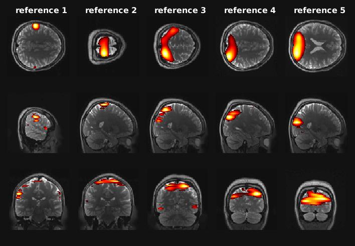
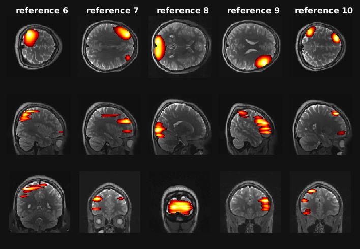
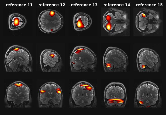
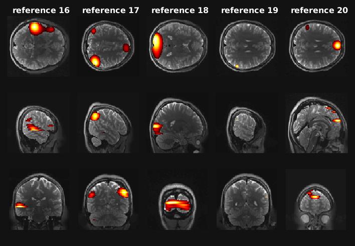
Figure 5: References used for cICA. The references are presented in the three principal anatomical planes: transverse, sagittal and frontal. The three planes intersect the voxel with highest intensity value in every volumetric image. For visualization purposes, the activations of the networks shown are normalized to zero mean and unit variance, and the intensity of the pictured brain slice $\hat{I}(\mathbf{r})$ was thresholded by $\hat{I}(\mathbf{r})>2$. The color range is adjusted to the largest intensity value in every pictured slice.

B.2 ICs obtained by the cICA - EMD approach

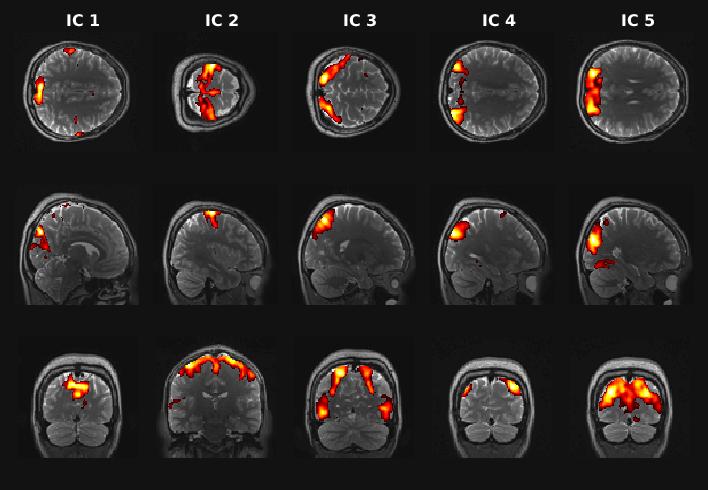
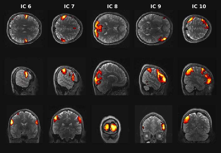
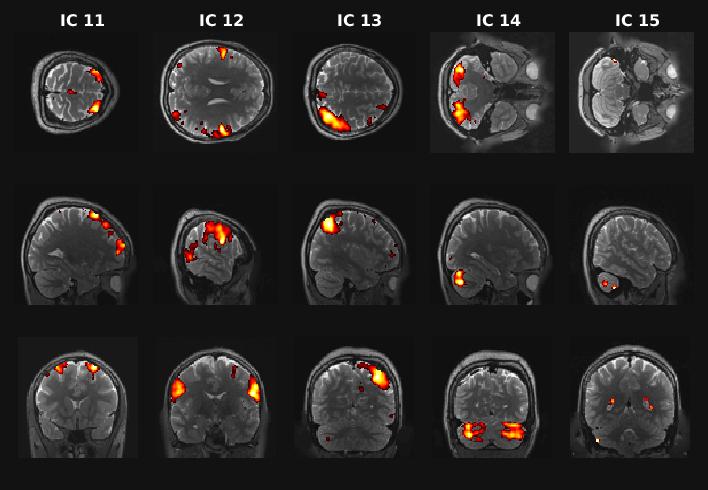
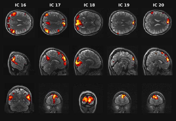
Figure 6: ICs obtained by the proposed approach. The depicted ICs are computed as mean ICs over subjects. Here the similarity threshold for cICA was set to $\mathbb{\varsigma}_{m}=0.5$. The ICs are presented in the three principal anatomical planes: transverse, sagittal and frontal. The three planes intersect the voxel with highest intensity value in every volumetric image. For visualization purposes, the activations of the networks shown are normalized to zero mean and unit variance, and the intensity of the pictured brain slice $\hat{I}(\mathbf{r})$ was thresholded by $\hat{I}(\mathbf{r})>2$. The color range is adjusted to the largest intensity value in every pictured slice.

B.3 ICs obtained by gICA

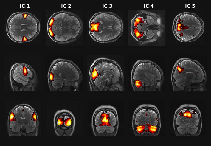
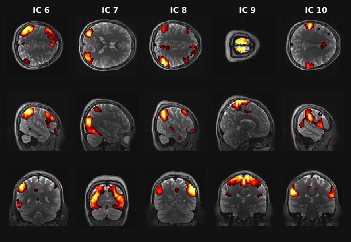
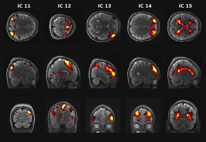
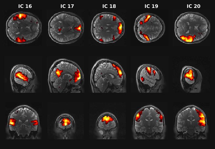
Figure 7: ICs obtained by gICA. The depicted ICs are computed as mean ICs over subjects. The ICs are presented in the three principal anatomical planes: transverse, sagittal and frontal. The three planes intersect the voxel with highest intensity value in every volumetric image. For visualization purposes, the activations of the networks shown are normalized to zero mean and unit variance, and the intensity of the pictured brain slice $\hat{I}(\mathbf{r})$ was thresholded by $\hat{I}(\mathbf{r})>2$. The color range is adjusted to the largest intensity value in every pictured slice.

References

- Al-Baddai et al. (2016a) S. Al-Baddai, K. Al-Subari, A. M. Tomé, B. Ludwig, D. Salas-Gonzales, and E. W. Lang. Analysis of fMRI images with bi-dimensional empirical mode decomposition based-on Green’s functions. Biomedical Signal Processing and Control, 30:53 – 63, 2016a. ISSN 1746-8094. doi: 10.1016/j.bspc.2016.06.019.
- Al-Baddai et al. (2016b) S. Al-Baddai, K. Al-Subari, A. M. Tomé, J. Sol-Casals, and E. W. Lang. A Green’s function-based Bi-dimensional empirical mode decomposition. Information Sciences, 348:305 – 321, 2016b. ISSN 0020-0255. doi: 10.1016/j.ins.2016.01.089.
- Allen et al. (2011) E. A. Allen, E. B. Erhardt, E. Damaraju, W. Gruner, J. M. Segall, R. F. Silva, M. Havlicek, S. Rachakonda, J. Fries, R. Kalyanam, A. M. Michael, A. Caprihan, J. A. Turner, T. Eichele, S. Adelsheim, A. D. Bryan, J. Bustillo, V. P. Clark, Feldstein Ewing, Sarah W., F. Filbey, C. C. Ford, K. Hutchison, R. E. Jung, K. A. Kiehl, P. Kodituwakku, Y. M. Komesu, A. R. Mayer, G. D. Pearlson, J. P. Phillips, J. R. Sadek, M. Stevens, U. Teuscher, R. J. Thoma, and V. D. Calhoun. A Baseline for the Multivariate Comparison of Resting-State Networks. Frontiers in Systems Neuroscience, 5, 2011. ISSN 16625137. doi: 10.3389/fnsys.2011.00002.
- Allen et al. (2014) E. A. Allen, E. Damaraju, S. M. Plis, E. B. Erhardt, T. Eichele, and V. D. Calhoun. Tracking whole-brain connectivity dynamics in the resting state. Cerebral cortex (New York, N.Y. : 1991), 24(3):663–76, 2014. ISSN 1460-2199. doi: 10.1093/cercor/bhs352.
- Beckmann and Smith (2005) C. Beckmann and S. Smith. Tensorial extensions of independent component analysis for multisubject fMRI analysis. NeuroImage, 25(1):294 – 311, 2005. ISSN 1053-8119. doi: 10.1016/j.neuroimage.2004.10.043.
- Bell and Sejnowski (1995) A. J. Bell and T. J. Sejnowski. An information-maximization approach to blind separation and blind deconvolution. Neural Computation, 7(6):1129–1159, Nov 1995. ISSN 0899-7667. doi: 10.1162/neco.1995.7.6.1129.
- Biswal and Ulmer (1999) B. B. Biswal and J. L. Ulmer. Blind source separation of multiple signal sources of fMRI data sets using independent component analysis. Journal of computer assisted tomography, 23 2:265–71, 1999.
- Calhoun et al. (2001a) V. D. Calhoun, T. Adali, V. B. McGinty, J. J. Pekar, T. D. Watson, and G. D. Pearlson. fMRI activation in a visual-perception task: Network of areas detected using the general linear model and independent components analysis. NeuroImage, 14:1080–1088, 2001a.
- Calhoun et al. (2001b) V. D. Calhoun, T. Adalı, G. D. Pearlson, and J. J. Pekar. A method for making group inferences from functional MRI data using independent component analysis. Human brain mapping, 14 3:140–51, 2001b.
- Calhoun et al. (2009) V. D. Calhoun, J. Liu, and T. Adalı. A review of group ICA for fMRI data and ica for joint inference of imaging, genetic, and ERP data. NeuroImage, 45 1 Suppl:S163–72, 2009.
- Cardoso (1997) J. F. Cardoso. Infomax and maximum likelihood for blind source separation. IEEE Signal Processing Letters, 4(4):112–114, 1997. doi: 10.1109/97.566704.
- Correa et al. (2007) N. Correa, T. Adalı, and V. D. Calhoun. Performance of blind source separation algorithms for fmri analysis using a group ica method. Magnetic Resonance Imaging, 25(5):684 – 694, 2007. ISSN 0730-725X. doi: 10.1016/j.mri.2006.10.017.
- Erhardt et al. (2011) E. B. Erhardt, S. Rachakonda, E. J. Bedrick, E. A. Allen, T. Adalı, and V. D. Calhoun. Comparison of multi-subject ICA methods for analysis of fMRI data. Human brain mapping, 32 12:2075–95, 2011.
- Esposito et al. (2005) F. Esposito, T. Scarabino, A. Hyvarinen, J. Himberg, E. Formisano, S. Comani, G. Tedeschi, R. Goebel, E. Seifritz, and F. D. Salle. Independent component analysis of fMRI group studies by self-organizing clustering. NeuroImage, 25(1):193 – 205, 2005. ISSN 1053-8119. doi: 10.1016/j.neuroimage.2004.10.042.
- Essen et al. (2012) D. V. Essen, K. Ugurbil, E. Auerbach, D. Barch, T. Behrens, R. Bucholz, A. Chang, L. Chen, M. Corbetta, S. Curtiss, S. D. Penna, D. Feinberg, M. Glasser, N. Harel, A. Heath, L. Larson-Prior, D. Marcus, G. Michalareas, S. Moeller, R. Oostenveld, S. Petersen, F. Prior, B. Schlaggar, S. Smith, A. Snyder, J. Xu, and E. Yacoub. The human connectome project: A data acquisition perspective. NeuroImage, 62(4):2222 – 2231, 2012. ISSN 1053-8119. doi: 10.1016/j.neuroimage.2012.02.018.
- Feinberg et al. (2010) D. Feinberg, S. Moeller, S. M Smith, E. Auerbach, S. Ramanna, M. Günther, M. F Glasser, K. Miller, K. Ugurbil, and E. Yacoub. Multiplexed echo planar imaging for sub-second whole brain fmri and fast diffusion imaging. 5:e15710, 12 2010.
- Fischl (2012) B. Fischl. Freesurfer. NeuroImage, 62(2):774 – 781, 2012. ISSN 1053-8119. doi: 10.1016/j.neuroimage.2012.01.021. 20 YEARS OF fMRI.
- Fox and Raichle (2007) M. D. Fox and M. E. Raichle. Spontaneous fluctuations in brain activity observed with functional magnetic resonance imaging. Nat Rev Neurosci, 8(9):700–711, 2007. ISSN 1471-003X.
- Glasser et al. (2013) M. Glasser, S. Sotiropoulos, J. Anthony Wilson, T. Coalson, B. Fischl, J. L Andersson, J. Xu, S. Jbabdi, M. Webster, J. Polimeni, V. Essen DC, and M. Jenkinson. The minimal preprocessing pipelines for the human connectome project. 80:105, 10 2013.
- Griffanti et al. (2014) L. Griffanti, G. Salimi-Khorshidi, C. F. Beckmann, E. J. Auerbach, G. Douaud, C. E. Sexton, E. Zsoldos, K. P. Ebmeier, N. Filippini, C. E. Mackay, S. Moeller, J. Xu, E. Yacoub, G. Baselli, K. Ugurbil, K. L. Miller, and S. M. Smith. ICA-based artefact removal and accelerated fMRI acquisition for improved resting state network imaging. NeuroImage, 95:232 – 247, 2014. ISSN 1053-8119. doi: 10.1016/j.neuroimage.2014.03.034.
- Harshman and Lundy (1994) R. Harshman and M. Lundy. PARAFAC: parallel factor analysis. Comput. Stat. Data Anal., 18:39 – 72, 1994.
- Himberg et al. (2004) J. Himberg, A. Hyvärinen, and F. Esposito. Validating the independent components of neuroimaging time series via clustering and visualization. NeuroImage, 22 3:1214–22, 2004.
- Hyvärinen et al. (2001) A. Hyvärinen, J. Karhunen, and E. Oja. Independent Component Analysis, volume 26. 06 2001. ISBN 9780471405405.
- Jenkinson et al. (2002) M. Jenkinson, P. Bannister, M. Brady, and S. Smith. Improved optimization for the robust and accurate linear registration and motion correction of brain images. NeuroImage, 17(2):825 – 841, 2002. ISSN 1053-8119. doi: 10.1006/nimg.2002.1132.
- Jenkinson et al. (2012) M. Jenkinson, C. F. Beckmann, T. E. Behrens, M. W. Woolrich, and S. M. Smith. FSL. NeuroImage, 62(2):782 – 790, 2012. ISSN 1053-8119. doi: 10.1016/j.neuroimage.2011.09.015. 20 YEARS OF fMRI.
- Jolliffe (2014) I. Jolliffe. Principal Component Analysis. American Cancer Society, 2014. ISBN 9781118445112. doi: 10.1002/9781118445112.stat06472.
- Kuhn (1955) H. Kuhn. The hungarian method for the assignment problem. 2:83–98, 01 1955.
- Lee et al. (1999) T.-W. Lee, M. A. Girolami, and T. J. Sejnowski. Independent component analysis using an extended infomax algorithm for mixed sub-gaussian and super-gaussian sources. Neural computation, 11 2:417–41, 1999.
- Lin et al. (2007) Q.-H. Lin, Y.-R. Zheng, F. Yin, H. Liang, and V. D. Calhoun. A fast algorithm for one-unit ICA-R. Inf. Sci., 177:1265–1275, 2007.
- Lin et al. (2009) Q.-H. Lin, J. Liu, Y.-R. Zheng, H. Liang, and V. Calhoun. Semiblind spatial ICA of fMRI using spatial constraints. 31:1076–88, 07 2009.
- Lu and Rajapakse (2006) W. Lu and J. C. Rajapakse. ICA with Reference. Neurocomputing, 69:2244–2257, 2006.
- McKeown et al. (1998) M. J. McKeown, T. P. Jung, S. Makeig, G. E. Brown, S. Kindermann, T. W. Lee, and T. J. Sejnowski. Spatially independent activity patterns in functional MRI data during the stroop color-naming task. Proceedings of the National Academy of Sciences of the United States of America, 95 3:803–10, 1998.
- Moeller et al. (2010) S. Moeller, E. Yacoub, C. A. Olman, E. Auerbach, J. Strupp, N. Y. Harel, and K. Ugurbil. Multiband multislice ge-epi at 7 tesla, with 16-fold acceleration using partial parallel imaging with application to high spatial and temporal whole-brain fmri. Magnetic resonance in medicine, 63 5:1144–53, 2010.
- Munkres (1957) J. Munkres. Algorithms for the assignment and transportation problems. Journal of the Society for Industrial and Applied Mathematics, 5:32–38, 03 1957.
- Nunes et al. (2003) J. C. Nunes, Y. Bouaoune, É. Deléchelle, O. Niang, and P. Bunel. Image analysis by bidimensional empirical mode decomposition. Image Vision Comput., 21:1019–1026, 2003.
- Remes et al. (2011) J. J. Remes, T. Starck, J. Nikkinen, E. Ollila, C. F. Beckmann, O. Tervonen, V. Kiviniemi, and O. Silven. Effects of repeatability measures on results of fMRI sICA: a study on simulated and real resting-state effects. NeuroImage, 56(2):554–69, 2011. ISSN 1095-9572. doi: 10.1016/j.neuroimage.2010.04.268.
- Rodriguez et al. (2014) P. A. Rodriguez, M. Z. Anderson, X.-L. Li, and T. Adalı. General non-orthogonal constrained ICA. IEEE Transactions on Signal Processing, 62:2778–2786, 2014.
- Salimi-Khorshidi et al. (2014) G. Salimi-Khorshidi, G. Douaud, C. F. Beckmann, M. F. Glasser, L. Griffanti, and S. M. Smith. Automatic denoising of functional MRI data: Combining independent component analysis and hierarchical fusion of classifiers. NeuroImage, 90:449 – 468, 2014. ISSN 1053-8119. doi: 10.1016/j.neuroimage.2013.11.046.
- Schmithorst and Holland (2004) V. J. Schmithorst and S. K. Holland. Comparison of three methods for generating group statistical inferences from independent component analysis of functional magnetic resonance imaging data. Journal of Magnetic Resonance Imaging, 19(3):365–368, 2004. doi: 10.1002/jmri.20009.
- Setsompop et al. (2012) K. Setsompop, B. Gagoski, J. R. Polimeni, T. Witzel, V. J. Wedeen, and L. L. Wald. Blipped-controlled aliasing in parallel imaging for simultaneous multislice echo planar imaging with reduced g-factor penalty. Magnetic resonance in medicine, 67 5:1210–24, 2012.
- Smith et al. (2013) S. M. Smith, C. F. Beckmann, J. Andersson, E. J. Auerbach, J. Bijsterbosch, G. Douaud, E. Duff, D. A. Feinberg, L. Griffanti, M. P. Harms, M. Kelly, T. Laumann, K. L. Miller, S. Moeller, S. Petersen, J. Power, G. Salimi-Khorshidi, A. Z. Snyder, A. T. Vu, M. W. Woolrich, J. Xu, E. Yacoub, K. Uğurbil, D. C. V. Essen, and M. F. Glasser. Resting-state fMRI in the human connectome project. NeuroImage, 80:144 – 168, 2013. ISSN 1053-8119. doi: 10.1016/j.neuroimage.2013.05.039.
- Svensén et al. (2002) M. Svensén, F. Kruggel, and H. Benali. ICA of fMRI group study data. NeuroImage, 16 3 Pt 1:551–63, 2002.
- van den Heuvel and Pol (2010) M. M. H. P. van den Heuvel and H. E. H. Pol. Exploring the brain network: a review on resting-state fmri functional connectivity. European neuropsychopharmacology : the journal of the European College of Neuropsychopharmacology, 20 8:519–34, 2010.
- Wessel and Bercovici (1998) P. Wessel and D. Bercovici. Interpolation with splines in tension: A Green’s function approach. 30:77–93, 01 1998.
- Xu et al. (2012) J. Xu, S. Moeller, J. Strupp, E. Auerbach, L. Chen, D. A. Feinberg, K. Ugurbil, and E. Yacoub. Highly accelerated whole brain imaging using aligned-blipped-controlled-aliasing multiband EPI. Proceedings of the 20th Annual Meeting of ISMRM, page 2036, 2012.