K3 surfaces from configurations of six lines in
and mirror symmetry II
— -functions —
Abstract.
We continue our study on the hypergeometric system which describes period integrals of the double cover family of K3 surfaces. Near certain special boundary points in the moduli space of the K3 surfaces, we construct the local solutions and determine the so-called mirror maps expressing them in terms of genus two theta functions. These mirror maps are the K3 analogues of the elliptic -function. We find that there are two non-isomorphic definitions of the lambda functions corresponding to a flip in the moduli space. We also discuss mirror symmetry for the double cover K3 surfaces and their higher dimensional generalizations. A follow up paper will describe more details of the latter.
1. Introduction
Consider elliptic curves given as double covers over branched along four points in general positions. These curves define a family of elliptic curves over the configuration space of four points in , which is called Legendre family. The elliptic lambda function is a modular function associated to this family. This gives the uniformization of the period map defined as a multi-valued function from to the upper-half plane . In this paper we will define a generalization of this elliptic lambda function for a certain family of K3 surfaces.
We will consider double covers of branched along six lines in general positions which are singular at fifteen intersection points of the lines. Blowing-up at the singularities gives smooth K3 surfaces over the configuration space of six lines, which we called double cover family of K3 surfaces in the previous work [17]. This family has been studied in many contexts (see [24] for example) as a natural generalization of the Legendre family over . In particular, in [20], monodromy property of the period map has been determined completely. However since the moduli space is singular, we need to find suitable resolutions to study throughly the analytic properties of the period maps. In [17], we have found nice resolutions and from the viewpoint of mirror symmetry and Picard-Fuchs differential equations of period integrals. The aim of this paper is to define K3 analogues to the elliptic lambda function based on these resolutions.
Let us recall that, for the definition of the the elliptic lambda function, the hypergeometric series
| (1.1) |
and the differential equation (Picard-Fuchs equation) satisfied by it plays a central role. In this case, Picard-Fuchs differential equation is given by Gauss’s hypergeometric differential equation, and its solutions determine the period integrals of the Legendre family. The period map is basically given by the ratio of the solutions with the monodromy group the congruence subgroup of . The elliptic lambda function is the inverse map with suitable boundary properties near the cusps. The following explicit forms for the lambda function and the hypergeometric series are well-known:
| (1.2) |
where . See Section 2.2 for the definitions of theta functions.
The generalization to a family of K3 surfaces has been studied extensively in the ’90s [20, 19, 24]. However, it was not clear how to resolve the moduli space to construct analogues of the expressions (1.2). In [17], we have found natural resolutions and of which are related by a four dimensional flip. In this paper, corresponding to these resolutions, we will construct two definitions for K3 analogues of the elliptic lambda function; they differ in their behaviors near the exceptional divisors of the resolutions. We call these analogues K3 lambda functions and , respectively. These might be called K3 lambda maps precisely, but we continue to use the word “function” to indicate the generalization of elliptic lambda function.
The K3 lambda functions are naturally identified with the so-called mirror map [13, 14] for the family of K3 surfaces. In connection to this, we will also discuss mirror symmetry of the family; we will find that the mirror geometry is a (singular) K3 surface which is given as a double cover of a del Pezzo surface , a three point blow-up of .
Below we summarize the K3 lambda functions and hypergeometric series which we shall formulate in this paper.
K3 lambda function : The mirror map is given by with
| (1.3) | , | , | ||||||||||
| , | ||||||||||||
where
with given by
and
is the weight four theta function, see Appendix A.
K3 lambda function : The mirror map is given by with
| (1.4) | , | |||||||||
| , |
where
with given by
As is the case for the relation , the above equalities for and are local expressions, which will be multiplied by suitable weight factors under the monodromy transformations (or, equivalently, under the modular transformations). However the forms of lambda functions and given above are global functions defined over the resolutions and , respectively.
The construction of this paper is as follows. In Section 2, we will describe the Legendre family in a form which generalizes to the double cover family of K3 surfaces. In particular, we describe in detail the well-known action on of the symmetric group . Based on the commutative diagram (2.8), which is equivariant under , we shall characterize the lambda function and the property of the hypergeometric series (1.2). In Section 3, we summarize known-results about the double cover family of K3 surfaces including the results in our previous work [17]. We will then use them to formulate a master equation for our definition of the lambda functions. In Section 4, we summarize the generalized Frobenius method [13, 14] which describes the local solutions near certain special boundary points called large complex structure limit points (LCSLs). We also present an explicit form of period integrals of the family which is valid near the LCSLs. In Section 5. we will describe the period map using local solutions near the special boundary points. We will find a consistent form of the master equation with the local expression of the period maps. We then solve the master equation algebraically to obtain the K3 analogues of the lambda function. In Section 6, we will discuss the mirror geometry of the double cover family of K3 surfaces. Each section relies on previous results scattered in many works. We will present these in appendices. In Appendix C, we present some explicit formulas for the representation which is a generalization of the well-known representation . This is a byproduct of our arguments, but should be of some interest in its own right.
Acknowledgements: S.H. would like to thank for the warm hospitality at the CMSA at Harvard University where progress was made. S.H. is supported in part by Grant-in Aid Scientific Research (C 16K05105, S 17H06127, A 18H03668 S.H.). B.H.L and S.-T. Yau are supported by the Simons Collaboration Grant on Homological Mirror Symmetry and Applications 2015–2019.
2. The elliptic -function
2.1. Legendre family
The double cover family of K3 surfaces shares many properties with the corresponding family of elliptic curves, i.e. the Legendre family. It is helpful to summarize the well-known results of the Legendre family in the forms which generalize to the double cover family of K3 surfaces.
2.1.a. The configuration space of four points in . The Legendre family is a family of elliptic curves given as double covers of branched at four points in general position. To describe the family, let us introduce a data given by
where is the set of complex matrices. We denote its open dense subset by
with . For , we consider an elliptic curve branched at four points specified by :
Isomorphism classes of these elliptic curves are parametrized by the quotient space . This quotient is naturally compactified by the GIT quotient [4, 21] which is called the configuration space of four points on .
It is easy to see the isomorphism . In fact, in the quotient, any matrix can be transformed into the form with
which can be identified with the cross ratio of four points.
2.1.b. Perid integrals and Picard-Fuchs equation. The period integrals over cycles in are given by
| (2.1) |
where is the contraction with the Euler vector field They are solutions to the Picard-Fuchs equation, which is given by the hypergeometric system , i.e. the hypergometric system on Grassmannian [1, 7]. The hypergeometric system reduces locally to the so-called GKZ (Gel’fand-Kapranov-Zelevinski) system [8] when we represent an equivalence class by
| (2.2) |
This reduces the action on to the torus actions of the form which preserve the above form of the matrix , i.e.,
| (2.3) |
where (see [17, Sect.2.4] for more details). The GKZ system is described by the affine parameters , and is defined on a natural toric compactification of the parameter space. Following Sect. 3 of [17], it is easy to see . In particular, we arrive at the cross ratio
| (2.4) |
as an affine coordinate of . We write this coordinate as a monomial by introducing and . After scaling by the factor , it is easy to see that the period integral
| (2.5) |
satisfies the following differential equation, Picard-Fuchs equation,
| (2.6) |
with (cf. [17, Sect.3]). This differential equation has three regular singularities at , and the local solutions around are generated by the standard Frobenius method;
| (2.7) |
where with . Here the constant factors and are fixed to have integral monodromies for the analytic continuations of the solutions over . The ratio of the period integral defines the multi-valued period map , where is the upper half plane. The inverse of the period map is one of the simplest example of the so-called mirror map. In the present case, this mirror map coincides with the elliptic lambda function which is a modular function on the level two subgroup of .
2.2. Theta functions and semi-invariants
Using the local solutions of (2.6), we can describe the mirror map locally, for example, in terms of the -expansion with . For global properties, we use modular forms on , whose ring of even weights are known to be generated by classical theta functions and . It is useful to summarize the relation to the period map in the following diagram:
| (2.8) |
where is the period map and . The map is defined by semi-invariants of the GIT quotient which we describe in detail below.
2.2.a. Theta functions. We follow the standard definition of the theta functions: , and which satisfy one linear relation . To a parallel formula with the K3 case, we associate the theta functions to certain partitions as follows:
They have the (anti-)symmetry properties and
Using these, the linear relation becomes
| (2.9) |
2.2.b. Semi-invariants. According to geometric invariant theory [4], the map is defined by the ring generators of semi-invariants of the actions on . Concretely, it is given by with
where represent the minors of . These ’s satisfy the Plücker relation which corresponds to (2.9), and the period map makes the diagram (2.8) commute.
2.2.c. Affine coordinates from the level two structure. The period map is in fact a multi-valued map with its monodromy group giving the isomorphism . The symmetric group of order three acts naturally on as its aoutomorphisms. These come from the right actions of on by permutation matrices, which induce the following actions on the cross ratio (2.4);
Because of the non-trivial isotropy group , the group action actually reduces to the factor group . We will identify this factor group with the subgroup . The explicit forms of the automorphisms are summarized in the following table:
| (2.10) |
In what follows, we shall read the above automorphisms as the coordinate transformations between different affine charts which cover .
Lemma 2.1.
Let be any point represented by matrix . Then the following properties hold:
-
(1)
There is a right action by which brings into of the form:
(2.11) where is a regular matrix.
- (2)
Proof.
(1) The moduli space parametrizes the equivalence classes of semi-stable configurations of four points in . The claim follows from the fact that no three points coincide for a semi-stable configuration represented by . (2) Suppose has the form (2.11). Then we have
where is unique by the condition with given in (2.3). Since acts on the matrix entries by actions, the condition is retained. ∎
Let us introduce the following notation for ;
Based on Lemma 2.1, we define for the subset of by
| (2.12) |
Then we have for . This shows that and is an affine coordinate on it. We will denote by this affine open set with its coordinate function . Now, it is easy to see that we have the covering of by these affine open sets:
| (2.13) |
When we have for a configuration , the coordinate function of evaluates the same point by . By definition, these two values are related by .
Remark 2.2.
’s are anti-homomorphisms, , since .
2.3. Transformation properties of semi-invariants
Let us recall that the semi-invariants are homogeneous polynomials of matrix elements of . We will express these semi-invariants as some polynomials in the affine coordinate of , and describe the transformation properties of these polynomials under the coordinate changes . This simply reproduces the well-known properties of the elliptic lambda function for the Legendre family. However, this will become our guiding principle to define the K3 analogues of the elliptic lambda functions.
2.3.a. Polynomials . It is convenient to write as
introducing the ordered set . Assume has a special form with . For such , we define
It is easy to verify that ’s are polynomials of ; and they are given by
| (2.14) |
for and , respectively.
2.3.b. Semi-invariants in affine coordinates. We can express the semi-invariants for general in terms of the polynomial given in (2.14). Let us first note that, by definition, we have the following relation for :
| (2.15) |
where .
Proposition 2.3.
For such that , we have
| (2.16) | ||||
Proof.
Definition 2.4.
For such that , we define the ratio of the factors in (2.16) by
| (2.17) |
and call it the twist factor (or gauge factor) for the transition from to .
Explicitly, we calculate the twist factors in terms of for as follows:
| (2.18) |
Remark 2.5.
The meaning of the twist factor becomes clear in the definitions of period integrals (2.1) and (2.5). Let us write the period integral (2.1) by . Then, it is easy to see that the normalized period integral in (2.5) related to in general by
| (2.19) |
We leave the derivations of the above relations for the reader.
Lemma 2.6.
Proof.
Proposition 2.7.
The Picard-Fuchs equation transforms to
| (2.20) |
under the twist .
Proof.
It should be noted in the above proposition that the local solutions about have the same form for all three singularities. In particular, the origins are the so-called maximally unipotent monodromy points (or LCSLs), which correspond to the cusps in . This property comes from the fact that the -modules of the Picard-Fuchs equation around three singularities are all isomorphic. We will see that similar properties hold for the double cover family of K3 surfaces although the relevant -module becomes more complicated (cf. Proposition 4.1).
2.4. The elliptic lambda function
We describe the elliptic lambda function (1.2) by extending the projective relation
to an affine relation in . We will be brief since the subject is more or less classical. However, for our definition of K3 lambda functions, the corresponding affine relations will play a central role.
2.4.a. Transformation properties of theta functions. The theta functions introduced in (2.2) are modular forms of weight two on . Let , be the standard generators of . The congruence subgroup is generated by and . For , which is given by composite of and , we denote its action on and by and , respectively. Then the transformation properties of the theta functions are determined by
Denote by the corresponding element of under a group isomorphism . When we fix the isomorphism by and , we can verify that the above transformation properties become
| (2.21) |
in the notation of Subsection 2.2, for . We also use the inverse relation of the isomorphism .
2.4.b. The elliptic lambda function from the affine relation. The period integral plays an important role in the following arguments.
Proposition 2.8.
Proof.
Note that this formal argument indicates that the product depends only on the class and defines a holomorphic function on . It should be noted however that the product is a multi-valued function which depends on the monodromy of the period integral . More precisely, we can use the equality (2.22) repeatedly from one chart to the other, but after the analytic continuation along a closed path coming back to , we do not necessarily have the original value because of the monodromy of the period integral .
The monodromy of the hypergeometric series (2.7) has a particular form
under the analytic continuation along a closed path with . We will not go into the detail, but only remark that this property comes from the fact that is a section of the Hodge bundle over .
Proposition 2.9.
Proof.
The first claim is immediate writing (2.23) explicitly. By definitions, we obtain three independent equations;
where we . Solving these equations for , we obtain and . The former is nothing but the which is defined by the inverse relation of . For the latter equality to be consistent, we must have the identity
which is a well-known relation in the classical theory of hypergeometric series. See [25, Sect.5.4] for a modern formulation.
The second claim follows the transformation property described in (2.22). Assume , then and we have since the diagram (2.8) is equivariant under action. Now for , the affine relation (2.23) is written by
Using and (2.21), we obtain
which is the relation imposed already on . Note that the set of points of the form is a Zariski open subset of . Therefore setting up the equations (2.23) around ( automatically produces the corresponding equations for all other affine chart . ∎
The affine relation (2.23) is the one which we will generalize to define the K3 lambda functions in the next section.
3. The master equation for the functions
3.1. Double cover family of K3 surfaces
Let us briefly recall the definition of a family of K3 surfaces branched along six lines in general position in , which we called double cover family of K3 surfaces in [17]. We denote six lines in by with the following linear forms:
When these lines are in general position, the double cover branched along these six lines defines a singular K3 surface with singularities at each 15 intersection points . Blowing-up these 15 singularities, we have a smooth K3 surface of Picard number 16 generated by the hyperplane class from and the curves of the exceptional divisors of the blow-up. The double cover family of K3 surfaces is a (four dimensional) family of K3 surfaces over the configuration space of six lines. The period integrals of this family and also their monodromy properties were studied extensively in a paper [20] by studying hypergeometric system . Also the configuration space of six lines in is a classical object in moduli problems. It is known that the compactification via geometric invariant theory [4] is isomorphic to Baily-Borel-Satake compactification [23, 18]. We will denote this isomorphic compactified moduli space by .
3.2. Period integrals
The double cover family of K3 surfaces is a natural generalization of the Legendre family of elliptic curves. Corresponding to the period integrals of the Legendre family, we have the period integrals of holomorphic two forms
| (3.1) |
where , and are integral (transcendental) cycles in ). The lattice of transcendental cycles is known [20] to be
| (3.2) |
where represents the hyperbolic lattice of rank 2, and is the root lattice of . The period integrals are parametrized by matrix representing six lines in general positions as follows:
As in the preceding section, making the dependence on the cycles implicit, we often write the period integral simply by . Let be the affine space of all matrices, and set
with representing minors of . Then, under the genericity assumption, the configurations of six lines are parametrized by
where represents the diagonal -actions.
Period integrals over the cycles define a multi-valued map, period map, from to the period domain
where represents one of the connected components. The period map naturally extends to the compactified moduli space of . In [20], the monodromy group of the period map has been determined to be the congruence subgroup of
where and . The group is a discrete subgroup of . It is known [20, Prop. 2.8.2] that for the quotient, where is the symmetric group of degree six.
3.3. Moduli space and the period map
The moduli space is a well-studied object in many contexts. We refer to [17, Sect.2.3] for a brief summary on this space and references. Here we summarize some properties of the moduli space and the period map of the family.
3.3.a. Baily-Borel-Satake compactification and the period map. The Baily-Borel-Satake compactification is described by an arithmetic quotient of the domain
where . The Siegel half space is defined by . Given a matrix , we have ten theta functions with even spin structures (see Appendix A for their explicit forms). With these theta functions we define a map
using the same letter as in (2.8). These squares of theta functions are modular forms of weight two on the modular subgroup of the discrete subgroup of . See [19, Sect. 3] for more details. On the other hand, using the semi-invariants for the left action on matrices , we have a natural map which gives the following commutative diagram [19, Thm. 4.4.1]:
| (3.3) |
As before, we code the semi-invarinats by the ordered partitions of so that we have
| (3.4) |
where the bracket represents the minor of matrix of with the specified columns. We assume the same sign changes of under the permutations of as the r.h.s of (3.4). Just as in the case of the Legendre family, we shall take the relation
as the guiding equation to define the K3 analogue of the lambda function. One might expect that the same arguments as the elliptic lambda function given in Section 2.4 hold for the double cover family of K3 surfaces. However, a crucial difference is that the moduli space is not smooth like . To define the K3 lambda functions, we need to find suitable resolutions of the singularity of which we have done in [17].
3.3.b. Singularities of . It is known that is singular along 15 lines of singularities. These lines intersect at 15 points, each of which is given as a transversal intersection of three lines. The configuration of these 15 lines is shown in Fig. 5 of [17]. From the 15 lines, we can select a maximal set of non-intersecting lines. Constructing the maximal set explicitly, we see that every maximal set consists of 5 lines, and furthermore, there are six possibilities for the maximal sets.
Proposition 3.1.
The following properties hold:
-
(1)
.
-
(2)
The group acts on the six maximal set of non-intersecting lines.
-
(3)
The group acts transitively on the 15 singular points.
Proof.
Proposition 3.2.
The symmetric group in the preceding proposition is identified with the natural action on coming from the action on matrix from the right. Under this identification, the diagram (3.3) is equivariant.
Lemma 3.3.
The singularities near the 0-dimensional boundary points are locally isomorphic to the singularity near the origin of
Proof.
This is proved in [17, Props.4.4, 6.5] ∎
In [17], we have described a resolution of the singularity, and also its (anti-)flip . The system expressed by the local coordinates of these two resolutions has a particularly nice property; there are LCSLs where we can define the mirror maps, i.e., the lambda functions. We refer to [17] for more details of the resolutions.
Proposition 3.4.
The action on extends to the resolutions and .
Proof.
The two resolution has been constructed by blowing-up along the 15 lines of the singularity followed by blow-ups at points. Since the blowing-up at points are local, they are compatible with the action. The (anti-)flip is made by (anti-)flipping the local resolution for all 15 isomorphic local geometry at one time. Hence, the resulting flip retains the action from . ∎
Let us recall the following covering property [17]:
| (3.5) |
where is a toric hypersurface in which is birational to , and is a divisor in . The toric hypersurface is singular along 9 lines of singularity, and these lines intersect at 6 points (cf. Lemma 3.3).
We will define our lambda functions, first locally, by the mirror maps given in the form of -expansions near the LCSLs in the local resolutions (or ) of . Then we will show that these local definitions actually extend to a global definition. To ensure that, we use Proposition 3.4 and the transformation property of some local expressions under the action. This is exactly parallel to the one we presented in the preceding section for the elliptic lambda function.
3.4. Defining functions
Recall that the equation (2.23) comes from the commutative diagram (2.8). We generalize this for the corresponding diagram (3.3).
3.4.a. LCSLs in and . For simplicity, let us write
in the decomposition (3.5) of . Since the component is isomorphic to a Zariski open subset of a toric variety , a general point is represented by a matrix having the properties
| (3.6) |
for a unique . The open subset contains six copies of the local geometry . We will identify one of them with , and denote it by . We denote its resolutions by and .
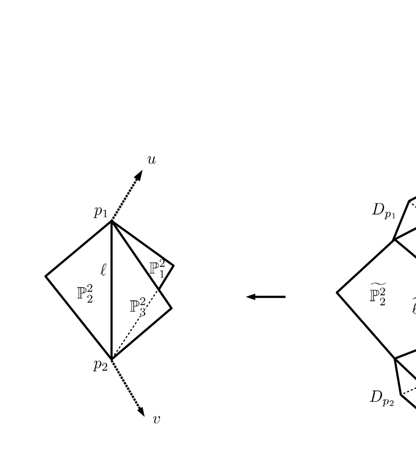
In Fig.1, it is shown that the resolution contains two LCSLs, . The left figure of Fig.1 is the blow-up along three coordinate axes that introduces corresponding exceptional divisors . The right figure represents the resolution by the blow-up at two points which introduces the exceptional divisors . The two LCSLs are given by the intersections of and the proper transforms of the three exceptional divisors. We introduce local coordinate near the point so that
are the local equations for the divisors and , respectively. Near the other point we introduce local coordinate in a similar way except that represents the divisor .
The transforms of the local geometry by the automorphisms , where [17, Def. 6.8], are all isomorphic. We set and denote by the resolution which is isomorphic to the resolution . Similarly for the other resolution . We denote by and , respectively, the corresponding local coordinates of the resolutions and . When , we often omit the superscript, e.g., .
Proposition 3.5.
The coordinate functions evaluate the general points by
| (3.7) |
where are determined by (3.6) from by choosing a matrix such that . These are independent of the representative of .
Proof.
The coordinate functions are determined in Lemma 3.3 of [17] as the generators of the coordinate ring of the affine coordinate around of the resolution . For a matrix such that , assume the matrix has the form (3.6), then the claimed form (3.7) follows by the definitions given in [17, Sect. 3.2.b]. Let us write . If we change to by , then we have with . It is easy to find a diagonal matrix satisfying , and we have . Since is the torus action on described in [17, Sect. 2.4.a] (see also Sect. 4.1 below), the values of the coordinate functions do not change for and . ∎
Proposition 3.6.
The coordinate functions are related to by
| (3.8) |
Proof.
This follows directly from Lemma 3.3 of [17]. Using the definitions there, the generators of the cone determine the coordinate functions . We read the coordinate functions from the generators of the cone . ∎
Remark 3.7.
Clearly, the decomposition (3.5) is a generalization of the corresponding decomposition (2.13) of . By similar arguments done for the coordinate functions on , the coordinate functions and are related by for (see Subsection 2.2). This generalizes the classical representation (2.10) of on . Unfortunately, the relations are not simple enough to list them in a table. In Appendix C, we show them explicitly for some .
The flipped resolution contains three LCSLs, which arises as the transversal intersections of four divisors. We will denote the corresponding coordinates by and for . See Appendix K3 surfaces from configurations of six lines in and mirror symmetry II — -functions — for the explicit descriptions of these local coordinates.
3.4.b. Semi-invariants in the affine coordinates . In what follow, we will focus on the boundary points given by . For simplicity, we write by unless otherwise stated. Also we write by . Then, for a general matrix , the expression represents the ratios (3.7) defined by making the matrix into the form (3.6). As in the table (2.10) in the preceding section, we have
Definition 3.8.
Take a special form with . Using this, we define affine semi-invariants by
where is the semi-invariants in (3.3).
The above definition is parallel to the case of . It is straightforward to find that these affine semi-invariants are polynomial functions of (defined for ). See Appendix B for their explicit expressions.
Proposition 3.9.
For a general matrix such that , the following equalities hold:
Proof.
Since the derivations are parallel to Proposition 2.3, we omit them here.∎
Definition 3.10.
For a general matrix such that , we define
and call this a twist factor (cf. Definition 2.4). We also set .
The following definition coincides with the normalized period integral [17, (3.4)] which corresponds to (2.5).
Definition 3.11.
For a general matrix such that , we define the normalized period integral
| (3.9) |
3.4.c. The master equation for the functions. We introduce the master equation by which we define the functions.
Proposition 3.12.
Proof.
Derivations are parallel to Proposition 2.8. ∎
Now we extend the projective relation in (3.3) to
Definition 3.13 (Master Equation).
The master equation (3.11) generalizes the equation (2.23) which characterizes the elliptic lambda function together with the classical relation for the hypergeometric series (1.1). In the following sections, we will find that the mirror map and the unique (up to constant) hypergeometric series near the LCSL satisfy the above master equation (Subsection 5.2 and Subsection 5.3).
Remark 3.14.
When we use the local coordinates for the other LCSL in the resolution , we will have the master equation in the same form as above. However, the polynomials of by the coordinate differ from those given above. Namely, we have
| (3.12) |
with different polynomials and for the coordinates and , respectively. It is straightforward to see that the following simple relation holds:
| (3.13) |
4. Generalized Frobenius method for local solutions
As studied in [13, 14], the GKZ hypergeometric systems in mirror symmetry are resonant and the mirror correspondence is encoded in the special form of local solutions expressed using Frobenius method, which generalizes the classical method for ordinary hypergeometric differential equations to GKZ hypergeometric systems of multi-variables. Since several new features can be observed in this generalization, e.g. Remark 4.6 below, we will call it the generalized Frobenius method when we emphasize them.
4.1. GKZ hypergeometric system from
At least locally, following [13, 14], we can describe the period map by using local solutions of Picard-Fuchs equation near the LCSL As in the preceding section, restricting our attentions to the neighborhood of , we simply write by for .
The Picard-Fuchs differential operators have been determined from the GKZ system associated to the system [17]. The GKZ system arises form the system by taking the following special form of a matrix :
| (4.1) |
This form reduces the left action on to the residual subgroup action of the diagonal tori . Taking into account the action from the right, we define
where with For the matrix , we have the following form of the period integral:
| (4.2) | ||||
Recognizing a striking similarities of (4.2) with the equations we encountered in [13], we observed that the period integral satisfies GKZ -hypergeometric system with a suitable choice of the finite set (see [17, Prop.3.1]).
For a general matrix , it holds that and . The normalized period integral (3.9) is given by
where we should identify , respectively, with (cf. (3.6)), and we have chosen the affine coordinate centered at the LCSL . The following proposition is described in [17, Prop. 3.6, Appendix C]:
Proposition 4.1.
The normalized period integral satisfies the Picard-Fuchs system which consists of differential equations with
| (4.3) |
where . Around the origin this system admits only one (up to constant) regular solution given by
with the coefficients given by
| (4.4) |
Remark 4.2.
The Picard-Fuchs system around the other point of the resolution simply follows from (4.3) by using the monomial relation (3.8). The Picard-Fuchs systems around the points of the are described in Appendix K3 surfaces from configurations of six lines in and mirror symmetry II — -functions —. The systems for the other boundary points follow from the above system by using the monomial relations described there.
4.2. Period integrals by the generalized Frobenius method
The Picard-Fuchs system is a complete set of differential equations which determines all local solutions around the origin . We construct all local solutions by Frobenius method for the hypergeometric system following [13, 14] (see Appendix D for a brief summary). The basic object is the indicial ideal which we can read off from (4.3).
Proposition 4.3.
Define the indicial ideal of the Picard-Fuchs system (4.3) by
This is a zero dimensional ideal in where .
Proof.
We verify the claimed property by calculating the Gröbner basis of . ∎
The fact that is a zero dimensional ideal is one of the properties for the origin to be a LCSL. The Picard-Fuchs system (4.3) has further properties which are common for the GKZ systems arising from mirror symmetry.
Proposition 4.4.
The quotient ring is of dimension 6, with its standard monomials . The intersection pairing (see Appendix K3 surfaces from configurations of six lines in and mirror symmetry II — -functions —) is given by
| (4.5) |
where will be fixed (to be 2) later.
Proof.
Since the indicial ideal is homogeneous, we have homogeneous basis for the quotient. We can determine the standard monomials by making Gröbner basis. The pairing follows form the definition of the -linear map described in Appendix K3 surfaces from configurations of six lines in and mirror symmetry II — -functions —. ∎
The following proposition is the content of the Frobenius method for hypergeometric series of multi-varibles.
Proposition 4.5.
(1) For the coefficient in (4.4), the following limits exist for all :
In particular, these are non-vanishing only for .
Proof.
Remark 4.6.
The solutions in (2) indicate that the classical Frobenius method for hypergeometric series of one variables naively extends to hypergeometric series of multi-varibles. This was the non-trivial observation first made in [13, 14] for GKZ hypergeometric systems arising from the mirror symmetry. In fact, it is easy to see that the limit has non-vanishing contributions even when some of ’s are negative. However, after summing up with , these contributions cancel out and we obtain the power series solution . In Appendix K3 surfaces from configurations of six lines in and mirror symmetry II — -functions —, we will show an example where a naive application of the Frobenius method for hypergeometric series of multi-variables generates local solutions but in the form of Laurent series.
4.2.a. Transcendental lattice from the period relation. Recall that generic members of our family of K3 surfaces have transcendental lattice (3.2). We can read off this transcendental lattice by finding a quadratic relation (period relation) satisfied by period integrals. Let us first look at the symmetric form on defined by matrix above (assuming is an integer).
Lemma 4.7.
The lattice with the symmetric form is isomorphic to , i.e., we have
Proof.
It is easy to verify that the unimodular matrix gives the isomorphism. ∎
Proposition 4.8.
The following quadratic relation holds:
| (4.6) |
Proof.
We verify this by series expansions of the solutions to some higher orders. ∎
When , using Lemma 4.7, we find that the above quadratic form and the form of the transcendental lattice are consistent if the following conjecture holds:
Conjecture 4.9.
Period integrals
| (4.7) |
are integral basis, i.e., have integral monodromy which preserve the symmetric form with .
Note that in this conjecture, we have introduced the factors to have integral local monodromy around the divisors . This integral structure of period integrals is in accord with the general formulas which come from mirror symmetry, see Appendix D. In Section 6, we describe the mirror geometry of using Proposition 4.8.
5. The functions from the master equation
We solve the master equation by determining the so-called mirror maps around the boundary point . Following the preceding section, we will first make a local analysis around the fixed boundary point . Using the transformation property of the master equation, we will finally arrive at the global expressions (1.3) and (1.4) for the functions.
5.1. Mirror maps
With the local solutions in Proposition 4.5, we can now define the mirror map locally around the point .
Definition 5.1.
(2) Putting , we write the inverse relations of (5.1) by
and call them the mirror map around the boundary point .
We set
Then it holds that for the period integrals (4.7). The quadratic relation (4.6) with becomes
where we define using the unimodular matrix in Lemma 4.7. This indicates that is a point in the period domain defined for the transcendental lattice , namely the map composed with the following isomorphism expresses the period map locally near the boundary point .
Lemma 5.2.
There is an isomorphism whose inverse is explicitly given by
for .
Proof.
It is easy to verify the quadratic relation . We refer [19, Sect. 1.3] for the more details of the isomorphism. ∎
Definition 5.3.
Remark 5.4.
Parallel to the above definition, we have local descriptions of the period maps near each of . Because of invariance of the resolutions and , we have local descriptions of the period maps near all of the boundary points in the resolutions as well.
When we study the modular properties, the coordinate introduced above is preferred to the coordinate . Correspondingly we define and which are related to the by
or by
| (5.2) |
Remark 5.5.
Here, the slightly mysterious shift in the definition corresponds to changing the branch cut for the logarithms of and , i.e., changing and in Definition 5.1. We do not have a good understanding about this shift, but this is necessary to express the mirror maps in terms of theta functions.
For convenience, we introduce the following notation.
Definition 5.6.
By we represent the mirror map substituted the relation (5.2), i.e., .
Proposition 5.7.
When we substitute the mirror map formally into the unique up to constant power series , we have
The above expression plays a role when studying the master equation.
5.2. Solving the master equation 1
Now we can set up the master equation around the boundary point by using the period map given in Definition 5.3 as follows:
where is the unique power series solution near . Note that both sides of this equation are given by -expansions when we substitute the mirror map . By explicit calculations, we find the following property:
Proposition 5.8.
When expanded into q-series, the master equation holds to some higher order in only if we take
Now we can determine (q) and in terms of the theta functions by solving the master equation
| (5.3) |
for , . This is an overdetermined algebraic system. However after some algebras, we find the following
Proposition 5.9.
The above master equation has a unique solution,
| (5.4) | , | , | ||||||||||
| , | ||||||||||||
| (5.5) |
where theta functions and are defined in Appendix A.
Proof.
Since the master equation (5.3) (for and ) is overdetermined, we select four equations to solve for . For example, we can take four equations indexed by the following
Using the corresponding polynomials in Appendix B, we obtain the claimed expressions (5.4). Substituting these into the remaining six equations, it turns out that these are equivalent to five linear relations among the theta functions [19, Rem. 3.1.2] and one additional equation;
We solve this equation for to obtain
where . Using the linear relations, we can verify the following equality:
where the second equality is nothing but the definition of the weight four modular form [19, Prop. 3.1.5]. We finally determine the sign of the square root so that the relation (5.6) below holds as the -series.∎
Remark 5.10.
We have solved the master equation (5.3) expressed in the coordinate around the boundary point . By the same arguments given in the proof of Proposition 2.9, we can transform the master equation (5.3) to other charts which cover , and see that these are equivalent to (5.3). For this argument, we use the covering property (3.5) of , the transformation property (3.10) and also the relation
for which corresponds to , see [19, Sect.3.1].
Proposition 5.11.
Clearly, the above relation is a generalization of the formula (1.2) which is classically known for the Legendre family. Several direct proofs are known for the relation in terms of Picard-Fuchs equations [25, Sect.5.4]. We do expect a similar direct proof for the above relation.
Remark 5.12.
The above analysis has been done starting from the local solutions around . We may also take the other boundary point , which are related by (Laurent) monomial relation (3.8). It is easy to see that the Picard-Fuchs system (4.3) preserves the same form when we substitute the monomial relation (3.8). Hence we obtain the same local solutions as in Propositions 4.1 and 4.5; and the same calculations as above apply to , and in particular, we result in the same form of the mirror map (5.4). However these two mirror maps have different boundary conditions; the former vanishes at the normal crossing divisors , while the latter vanishes at . We regard these mirror maps as different representations of a -function, which correspond to different forms of the elliptic -function, cf. (2.10), with different vanishing conditions at the cusps.
5.3. Solving the master equation 2.
Completely parallel calculations apply to the flipped resolution where we found three boundary points . We denote by the corresponding local coordinate and set . From the definitions and (see [17, Def.3.5]) and the relations (D.2), we see that the coordinate is related to the coordinate of the other resolution by
Inverting this (Laurent) monomial relation as , we substitute into the polynomials . We directly check the results are polynomials in .
Definition 5.13.
We define by the polynomial .
By definition, we have
It should be noted that and are polynomials of different shapes.
In Appendix A, we list the Picard-Fuchs system in the coordinate . The origin of this system is a LCSL where we have unique (up to constant) regular solution and all others contain powers of logarithms, . The Frobenius method applies to this case as well. By finding the quadratic relation satisfied by solutions, we can describe the period map locally around . This time we set up the master equation in the following from
| (5.7) |
Proposition 5.14.
When (5.7) is expanded in -series, the master equation holds in lower degrees in only when when we take
Using the above element , we set up the algebraic master equation for and . Corresponding to Proposition 5.9 ans Proposition 5.11, we obtain
Proposition 5.15.
The master equation has a unique solution,
| (5.8) | , | |||||||||||
| (5.9) |
where , and are defined in Appendix A.
Proposition 5.16.
Remark 5.17.
As above, we arrived at the two definitions of the K3 analogues of elliptic lambda functions, and corresponding to the resolutions and , respectively. As described in Remark 5.12, these two have different behavior near the normal crossing boundary divisors in the different resolutions and . We regards these and are non-isomorphic since these are defined on the non-isomorphic resolutions.
6. Mirror symmetry to a double cover of
We can read off a mirror correspondence of the K3 surfaces from the period integrals near the LCSLs (see Appendix D). Extending general observations made in [13, 14, 15] to the present case, we identify the mirror partner of starting from inspecting the structure of the ring defined by the indicial ideal .
6.1. A double cover of
Let be a blow-up at three (general) points of , which is a del Pezzo surface of degree 6. We denote by the exceptional divisors and by the pull-back of the hyperplane class in . Then following the lemma is immediate:
Lemma 6.1.
Define and . Then the intersection form is given by
| (6.1) |
We identify the above intersection form, up to the factor , with (4.5) appeared in Proposition 4.4. We explain the factor by considering a double cover: Consider two general elements for each one dimensional linear system on . We define the double cover branched along the zero locus .
Proposition 6.2.
The double cover of is a surface which is singular at 12 points of singularities. Its Picard lattice is generated by the proper transforms of with the intersection matrix .
Proof.
The number of intersection points is immediate by counting intersection numbers of the divisors The intersection forms are doubled by the double covering. ∎
The intersection form of explains the factor in Proposition 4.8. Let us recall that the K3 surface is defined to be a resolution of the singular double cover branched along general six lines. Based on the form of mirror symmetry observed for hypersurfaces in toric varieties [13, 12], we conjecture the following (cf. the next section):
Conjecture 6.3.
Mirror of the double cover (singular) K3 surface is a singular K3 surface defined above. Namely, the double covering of del Pezzo surface branched along the zero loci of general elements (i=1,2,3; a=1,2).
The relation of the conjecture to the standard descriptions of mirror symmetry of K3 surfaces [2, 5, 11] is not completely clear, since the lattice instead of is contained as a summand of the transcendental lattice , for example. However, we interpret below the conjecture as a variant of the so-called Batyrev-Borisov toric mirror construction.
6.2. Double coverings from the Batyrev-Borisov duality
It is suggestive to arrange the combinatorial data for the constructions and into a generalization of Batyrev-Borisov toric mirror construction [2, 3]. In a follow up paper [16], we will provide a full generalization to all dimensional Calabi-Yau varieties.
6.2.a. Batyrev-Borisov duality. Recall that, in toric geometry, the projective plane is described as with a two dimensional polytope
whose integral points represent sections of . We consider the following Minkowski sum decomposition
| (6.2) |
with and This decomposition corresponds to the factorization of Laurent polynomials of into polynomials defined for each polytope . In terms of homogeneous coordinates, this is nothing but a factorization of cubic polynomials into three linear polynomials.
According to Batyrev-Borisov construction, we define the following polar dual
Then, the Minkowski decomposition (6.2) induces the corresponding Minkowski decomposition of ,
with and . By Batyrev-Borisov duality, we obtain the original by the polar dual
The duality holds in general for the so-called reflexive polytopes with additional data called nef-partitions. In Fig.2, we summarize the duality in the present case. It is clear that the toric variety is isomorphic to , the blow-up at three coordinate points of .
6.2.b. Double coverings from the duality. In the Batyrev-Bosisov duality, associated to the polytope (respectively ), we have Laurent polynomial () and also a toric divisor in (in ). They may be summarized in
under the duality.
Definition 6.4.
Suppose two reflexive polytopes have Minkowski sum decompositions and which are dual in the sense of Batyrev-Borisov. Take two general sections and for each divisors and . We define the double covering of toric Fano variety branched along , and similarly of with the branch locus in .
By construction, the double covers and are Calabi-Yau varieties which is singular in general. Our observation made in Conjecture 6.3 can be understood as a special case of the pair of double covers in dimensions two, i.e., . We naturally expect that these double cover Calabi-Yau varieites and are mirror symmetric in general as we have observed in the special case. Other geometric justifications (e.g. [22, 9, 10, 6]) for this new duality are also expected, but we defer them to future investigations.
Appendix A Genus two theta functions
Definition A.1.
For and , we define theta functions on by
The theta functions used in the text are special types given by satisfying , which are specified by the correspondence
Explicitly, we use the following correspondences [19]:
We also write these ten theta functions by with by ordering the theta functions from the left to right, and the first line to the third line in the above correspondence. These functions have -series expansions with
for . The following properties are known in literatures (see [19, Prop.3.1.1, Cor. 3.2.2]):
Proposition A.2.
The squares of the ten theta functions are modular forms on with the character . Any five of linearly independent theta functions freely generate the module .
Appendix B The polynomials and
Recall that we have defined the polynomials and by expressing the (inhomogeneous) semi-invariants by the affine coordinates and , respectively. By definition, we have
The coding of the semi-invariants by comes from the definition . We use the definitions given in [17, Appendix C];
where is used for the degree two element. We denote by and the corresponding polynomials to the above. These numbering should not be confused with the numbering . Below we list the polynomials :
The polynomial is determined by by substituting the relations , . Note that are polynomials in although appears in the denominator of .
Appendix C The representation of
The right action of on matrix defines an element of , . This naturally gives rise to the well-known representation :
Here we have included the twist factor defined in (2.4). In a similar way, we have the representation induced by the right action of on matrices. This action naturally defines the corresponding transformation on the affine coordinates of the resolutions. For the case , we present explicit forms of the transformations for some . Although expressions become complicated in general, these should be regarded as the generalization of the rational transformations given in the above table.
We have similar expressions for the other boundary points and as well.
Appendix D Mirror symmetry and the generalized Frobenius method
Here we summarize briefly the Frobenius method formulated in [13, 14, 15] for the GKZ systems which determines period integrals of Calabi-Yau complete intersections. The (generalized) Frobenius method applies to the local solutions about special boundary points, i.e., LCSLs. Assume that is a K3 surface given as complete intersection in a toric variety, and is the mirror K3 surface determined by Batyrev-Borisov toric mirror symmetry [2, 3]. In this setting, we have a family of over the parameter space of its defining equations.
Let be the affine coordinate near a LCSL. Let be the Picard-Fuchs differential operators which follows from the GKZ system characterizing the period integrals in the affine chart. Following [13, 14, 15], we consider a polynomial ring generated by and define the indicial ideal of the Picard-Fuchs equations,
Indicial ideal is a homogeneous ideal generated by initial terms of and determines the indices for the local solutions.
Proposition D.1.
There is an isomorphism
where is generated by the restrictions of the ambient toric divisors.
When we normalize the top form of quotient ring, we can introduce a pairing in the quotient ring which corresponds to the pairing in the cohomology (of the mirror manifold). We denote this pairing for the generators by
This represents the intersection pairing among the corresponding generators of .
Proposition D.2.
Near the boundary point (LCSL), there is only one power series representing a period integral of the mirror family, which has the form . All other solutions contain logarithmic singularities, and they are given by
| (D.1) |
where with formal parameters .
Mirror symmetry of K3 surfaces can be summarized in the following proposition:
Proposition D.3.
[12, Sect. 2.4] The following quadratic relation holds:
Three propositions above provide a quick summary of the works [13, 14, 15] for the mirror symmetry expressed in the Frobenius method. It should be noted that, while the standard Frobenius method is a well-known technique for hypergeometric differential equations of one variables, the Frobenius method here is a non-trivial generalization to multi-variables, see Remark 4.6 and Appendix K3 surfaces from configurations of six lines in and mirror symmetry II — -functions — below.
Chapter \thechapter Proof of Proposition 4.5
Here we present the details of the proof of Proposition 4.5. We also include an example which shows that a naive application of Frobenius method results in Laurent series in general.
E1. Proof of 4.5. Let be the Picard-Fuchs differential operators in (4.3). Let be the homogeneous generators of the indicial ideal in Proposition 4.3, in order. Then, for the hypergeometric series defined in Proposition 4.5 (2), it is easy to verify that
where are the monomials with replaced by , and are power series in . The indicial ideal can be identified with the ideal of the polynomial ring . As claimed in Proposition 4.4, the quotient ring is finite dimensional with its bases . We can introduce a -linear map by the following properties
where is a constant. In Proposition 4.4, we have introduced . The next lemma follows from the above definitions:
Lemma D.4.
For , we have
If , then by definition. Therefore we have
for . These relations explain the form of local solutions in Proposition 4.5 (2), which generalizes the classical Frobenius method for hypergeometric series of one variable. See [14, Sect.3.3] and an example therein for more detailed analysis.
The vanishing described in Proposition 4.5 (1) depends on the special form of the coefficient :
Since vanishes when the -functions in the denominator have poles, it is easy to read off the necessary conditions for non-vanishing that and . From these conditions, we obtain , hence power series for . However that is a power series does not guarantee that is a power series. In the present case (and also for GKZ hypergeometric series near the LCSLs), we verify that this is the case directly. We express the derivation , for example, as
where . In this form we see that there are possibilities for the poles (of -functions) in the denominator of and the poles in the -functions cancel to result fine contributions. We write such possibilities for each terms; e.g., we have , and for . From these inequalities, we obtain and and conclude that they can have non-vanishing contributions only for . Doing similar analysis for the other terms, we conclude that the summation over in stays in the same range, i.e., . Hence we obtain the power series solution which is linear in . Since other cases are similar, although more involved for , we omit the details.
E2. Laurent series from the Frobenius method. As is clear in the above proof, in general, hypergeometric series of multi-variables can have some negative powers when we apply the Frobenius method. In this respect, the content of Proposition 4.5 (which goes back to the observations made in [13, 14]) is that negative powers do not appear for the special boundary points (LCSLs) coming from GKZ systems.
To contrast the situation, we present constructions of the local solutions of system with the affine parameter defined by
Yoshida et al [20, Prop.1.6.1] studies the system in this coordinate. Near the origin, , there is only one power series [20, Prop.1.6.2] which we translate to with
By explicit calculations, we can verify that all other solutions contains logarithms, and . For example, the solutions linear in is given by the naive application of the Frobenius method However this becomes a Laurent series as we can deduce from
By explicit calculation, we verify that the Laurent series
satisfies the system given in Yoshida et al [20, Prop.1.6.1]. Similar calculations works for the other logarithmic solutions as well.
Chapter \thechapter Picard-Fuchs operators for
There are three LCSLs in the flipped resolution . We introduce the local affine coordinates and whose origins are the LCSLs . Here, following Lemma 3.3 and Definition 3.5 of [17], we describe the coordinate and also Picard-Fuchs differential operators explicitly. Following the notation in [17], we first note that the cone is generated by
| (D.2) |
The coordinates follow from these by , i.e.,
It turns out that a complete set of differential operators are given by the following ’s (cf. [17, Appendix C]):
Setting , the operators take the following forms:
The radical of the discriminant is given by
The pairing from the quotient ring is determined as
with and fixing the normalization by (cf. Proposition 4.4). As in Proposition 4.5, we have local solutions around via the Frobenius method using the above . The corresponding quadratic relation also holds with replaced by in Proposition 4.8
As a unique (up to constant) solution, we obtain
with given by
The following proposition follows from constructing the integral generators of the semi-groups described in Lemma 3.3 of [17].
Proposition D.5.
The other two affine coordinates and are related to by
| (D.3) | ||||||||||
By using these relations, it is straightforward to express the Picard-Fuchs operators in the coordinates and also . We leave it to the reader to see that the set of operators has the same form for these three coordinates.
References
- [1] K. Aomoto, On the structure of integrals of power products of linear functions, Sci. Papers, Coll. Gen. Education, Univ. Tokyo, 27(1977), 49–61.
- [2] V. Batyrev, Dual polyhedra and mirror symmetry for Calabi-Yau hypersurfaces in toric varieties, J. Algebraic Geom., 3(3):493–535, 1994.
- [3] V. Batyrev and L. Borisov, On Calabi-Yau complete intersections in toric varieties, in “Higher-dimensional complex varieties (Trento, 1994)”, pages 39–65. de Gruyter, Berlin, 1996.
- [4] I. Dolgachev and D. Ortland, Points Sets in Projective Space and Theta Functions, Astérisque, vol.165, 1989.
- [5] I. Dolgachev, Mirror symmetry for lattice polarized K3 surfaces, Algebraic geometry, 4. J. Math. Sci. 81 (1996) 2599–2630.
- [6] C. Doran, A. Harder, A. Thompson, Mirror symmetry, Tyurin degenerations and fibrations on Calabi-Yau manifolds, in “String-Math 2015”, pages 93–131, Proc. Sympos. Pure Math., 96, Amer. Math. Soc., Providence, RI, 2017.
- [7] I.M. Gel’fand and M.I. Graev, Hypergeometric functions associated with the Grassmannian , Soviet Math. Dokl. 35 (1987) 298–303.
- [8] I.M. Gel’fand, A. V. Zelevinski, and M.M. Kapranov, Equations of hypergeometric type and toric varieties, Funktsional Anal. i. Prilozhen. 23 (1989), 12–26; English transl. Functional Anal. Appl. 23(1989), 94–106.
- [9] M. Gross and B. Siebert, Mirror symmetry via logarithmic degeneration data I. Journal of Differential Geometry, 72(2):169–338, 2006.
- [10] M. Gross and B. Siebert, Mirror symmetry via logarithmic degeneration data II, Journal of Algebraic Geometry, 19(4):679–780, 2010.
- [11] M. Gross, P.M.H. Wilson, Large complex structure limits of K3 surfaces, Journal of Differential Geometry, 55(3):475–546, 2000.
- [12] S. Hosono, Local Mirror Symmetry and Type IIA Monodromy of Calabi-Yau Manifolds, Adv. Theor. Math. Phys. 4 (2000), 335–376.
- [13] S. Hosono, A. Klemm, S. Theisen and S.-T. Yau, Mirror Symmetry, Mirror Map and Applications to complete Intersection Calabi-Yau Spaces, Nucl. Phys. B433(1995)501–554.
- [14] S. Hosono, B.H. Lian and S.-T. Yau, GKZ-Generalized hypergeometric systems in mirror symmetry of Calabi-Yau hypersurfaces, Commun. Math. Phys. 182 (1996) 535–577.
- [15] S. Hosono, B.H. Lian and S.-T. Yau, Maximal Degeneracy Points of GKZ Systems, J. of Amer. Math. Soc. 10 (1997), 427–443.
- [16] S. Hosono, B.H. Lian, T.-J. Lee and S.-T. Yau, work in progress.
- [17] S. Hosono,B.H. Lian, H. Takagi and S.-T. Yau, K3 surfaces from configurations of six lines in and mirror symmetry I, arXiv:1810.00606v1.
- [18] B. Hunt, The geometry of some special arithmetic quotients, Lect. Notes in Math. 1637 (1996) Springer-Verlag, Berlin Heidelberg.
- [19] K. Matsumoto, Theta functions on the bounded symmetric domain of type and the period map of a 4-parameter family of K3 surfaces, Math. Ann. 295 (1993) 383–409.
- [20] K. Matsumoto, T. Sasaki and M. Yoshida, The monodromy of the period map of a 4-parameter family of K3 surfaces and the hypergeometric function of type , Internat. J. Math. vol.3, No.1 (1992) 1 –164.
- [21] E. Reuvers, Moduli spaces of configurations, Ph.D. thesis (Radboud University, 2006), http://www.ru.nl/imapp/research_0/ph_d_research/
- [22] A. Strominger, S.-T. Yau and E. Zaslow, Mirror symmetry is T-Duality, Nucl. Phys. B479 (1996) 243–259.
- [23] G. van der Geer, On the Geometry of a Siegel Modular Threefold, Math. Ann. 260 (1982) 317–350.
- [24] M. Yoshida, Hypergeometric Functions, My Love – Modular Interpretations of Configuration Spaces–, Springer, 1997.
- [25] D. Zagier, Elliptic Modular Froms and Their Applications, in “The 1-2-3 of Modular Forms” by J.Bruiner, G. van der Geer, G. Harder and D. Zagier eds, Springer, 2008.
Department of Mathematics, Gakushuin University,
Mejiro, Toshima-ku, Tokyo 171-8588, Japan
e-mail: hosono@math.gakushuin.ac.jp
Department of Mathematics, Brandeis University,
Waltham MA 02454, U.S.A.
e-mail: lian@brandeis.edu
Department of Mathematics, Harvard University,
Cambridge MA 02138, U.S.A.
e-mail: yau@math.harvard.edu