Antiferromagnetism, Superconductivity and Phase Diagram in the
Two-Dimensional Hubbard Model
– Off-Diagonal Wave Function Monte Carlo Studies of Hubbard Model III –
Abstract
We investigate the ground-state phase diagram of the two-dimensional Hubbard model based on the optimization variational Monte Carlo method. We use a wave function that is an off-diagonal type given as , where is a one-particle state, is the Gutzwiller operator, is the kinetic operator, and is a variational parameter. The many-body effect plays an important role as an origin of spin correlation and superconductivity in correlated electron systems. We examine the competition between the antiferromagnetic state and superconducting state by varying the Coulomb repulsion , the band parameter and the electron density . We show a phase diagram that includes superconducting and antiferromagnetic phases and that is most favorable for superconductivity.
1 Introduction
The mechanism and properties of high-temperature superconductivity have been studied vigorously for more than 30 years since the discovery of cuprate high-temperature superconductors[1]. High-temperature cuprates are typical strongly correlated systems since the parent materials are Mott insulators when no carriers are doped. It is important to understand the electronic properties of strongly correlated electron systems because high-temperature cuprates are typical strongly correlated systems and the parent materials are Mott insulators when no carriers are doped.
The CuO2 plane commonly contained in high-temperature cuprates consists of oxygen atoms and copper atoms. The electronic model for this plane is given by the d-p model or three-band Hubbard model[2, 3, 4, 5, 6, 7, 8, 9, 10, 11, 12, 13, 14, 15, 16, 17, 18, 19, 20, 21, 22, 23, 24]. It appears very difficult to understand the ground-state phase diagram of the d-p model because of strong correlation between electrons. The two-dimensional (2D) single-band Hubbard model[25, 26, 27, 28, 29, 30, 31, 32, 33, 34, 35, 36, 37, 38, 39, 40, 41, 42, 43, 44, 45] has been investigated as a simplified model of the d-p model. The ladder model[46, 47, 48, 49, 50, 51] has also been studied in relation to the mechanism of superconductivity in a correlated electron system.
The Hubbard model is one of the fundamental models in condensed matter physics. It was first introduced to understand the metal-insulator transition[52] and is also used to describe the magnetic properties of various compounds[53, 54]. By employing the Hubbard model, we can understand the appearance of inhomogeneous states such as stripes[55, 56, 57, 58, 59, 60, 61, 62] and checkerboard-like density wave states[63, 64, 65, 66], whose existence was reported for high-temperature cuprates.
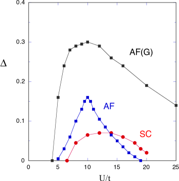
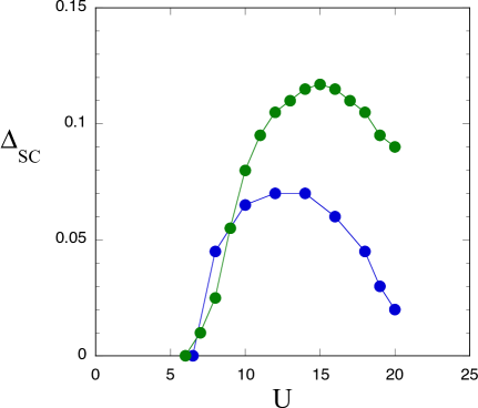
Recent studies on the 2D Hubbard model indicate that a superconducting (SC) phase exists in the ground state[45]. This shows the possibility that the 2D Hubbard model may account for high-temperature superconductivity. We show the order parameters of the antiferromagnetic (AF) state and SC state as a function of the interaction parameter in Fig. 1. The result shows that high-temperature superconductivity may occur in the strongly correlated region of the Hubbard model where the interaction is greater than the bandwidth.
A variational Monte Carlo method is a useful tool to investigate the electronic properties of strongly correlated electron systems when we calculate the expectation values numerically[32, 33, 34, 35, 36, 37]. In general, a variational wave function is improved by introducing new variational parameters to control the electron correlation. In our method the wave functions are optimized by multiplying an initial function by -type operators[45, 67], where is a suitable correlation operator. The Gutzwiller function is also written in this form. An optimization process is performed in a systematic way by multiplying by the exponential-type operators repeatedly[67]. The ground-state energy is indeed lowered considerably by using this type of wave function[45].
In this paper we investigate the stability of the antiferromagnetically ordered state and show the phase diagram of the ground state of the 2D Hubbard model. In the strongly correlated region, the AF correlation is suppressed and the SC correlation is enhanced. Near the boundary of the AF region, a large spin fluctuation is induced, which is considered to give rise to high-temperature superconductivity. The paper is organized as follows. In Sect. 2, we present the model Hamiltonian and wave functions that we use in the optimization variational Monte Carlo method. In Sect. 3, we examine the wave function with the AF order parameter to show the region where the AF state is stabilized. In Sect. 4, we discuss the phase separation that may occur near half-filling. In Sect. 5, we investigate the SC state and show the phase diagram. We give a summary in the final section.
2 Optimization Variational Monte Carlo Method
2.1 Hamiltonian
The Hubbard model is written as
| (1) |
where indicates the transfer integral and is the strength of the on-site Coulomb interaction. We set when and are nearest-neighbor pairs and when and are next-nearest-neighbor pairs. We consider this model in two dimensions, and and denote the number of lattice sites and the number of electrons, respectively. The energy unit is given by .
2.2 Off-diagonal wave function
In a variational Monte Carlo method, we employ a wave function that is suitable for the system being considered and evaluate the expectation values by using a Monte Carlo procedure. To take into account the correlation between electrons, we start from the Gutzwiller wave function given by
| (2) |
where is the Gutzwiller operator , where is the variational parameter in the range of . indicates a trial one-particle state.
Because the Gutzwiller function is very simple and is not enough to take account of electron correlation, we should improve the wave function. There are several methods to improve the wave function. One method is to multiply the Gutzwiller function by an exponential-type operator. The wave function is written as[45, 67, 68, 69, 70, 71, 72, 73]
| (3) |
where is the kinetic part of the Hamiltonian and is a real variational operator[37, 67, 69]. The expectation values are calculated by using the auxiliary field method[67, 74]. The other method is to introduce a Jastrow-type operator[39]. We control the nearest-neighbor correlation by multiplying by the operator
| (4) |
where is the operator for the doubly occupied site given as and is that for the empty site given by . is the variational parameter in the range . With this operator, we can include the doublon-holon correlation:
| (5) |
It is possible to generalize the Jastrow operator to consider long-range electron correlation by introducing new variational parameters[75, 76].
In this paper we use the wave function of the exponential type in eq. (3). We call this type of wave function the off-diagonal wave function since the off-diagonal correlation in the site representation is taken into account in this wave function. We believe that it is more important to consider off-diagonal electron correlation than the diagonal electron correlation. In fact, the energy is further lowered when we employ the off-diagonal wave function[45].
2.3 Antiferromagnetic state
The AF one-particle state is given by the eigenfunction of the AF trial Hamiltonian
| (6) |
where is the AF order parameter and represents the coordinates of site . The wave function is written as
| (7) |
In general, the AF state is very stable in the Hubbard model near half-filling. Thus, it is important to control the AF magnetic order so that the SC state is stabilized and realized.
The stability of the AF state depends mainly on the electron density , the interaction strength , the transfer integral , and long-range transfers in the single-band Hubbard model. The AF correlation is induced as increases from zero in the weakly correlated region and is maximized when is of the order of the bandwidth, say at , when carriers are doped. When becomes larger than , the AF correlation starts to decrease. In the region where is extremely large, the AF correlation is suppressed to a small value by the large fluctuation. This is shown in Fig. 1. This is a crossover between the weakly correlated region and strongly correlated region.
2.4 Correlated superconducting state
The SC state is represented by the BCS wave function
| (8) |
with coefficients and that appear in the ratio , where is the gap function with dependence and is the dispersion relation of conduction electrons. We assume -wave symmetry for : . The Gutzwiller BCS state is formulated as
| (9) |
where indicates the operator used to extract the state with electrons. In this wave function the electron number is fixed and thus the chemical potential in is regarded as a variational parameter. In the formulation of , we use the BCS wave function without fixing the total electron number, namely, without the operator . The chemical potential in is not a variational parameter and is used to adjust the total electron number. The wave function is given as
| (10) |
We perform the electron-hole transformation for down-spin electrons:
| (11) |
and not for up-spin electrons: . The electron pair operator denotes the hybridization operator in this formulation.
3 Antiferromagnetic phase
Since the SC state competes with the AF state, it is important to clarify the region of the AF state in the parameter space. We use and to control the strength of the AF correlation. The Coulomb interaction is important since the magnitude of the AF magnetism can be controlled by changing . The transfer integral is also important and shows nontrivial effect on the stability of the AF magnetic order. One may expect that the AF region will be small when including in the model. This is not, however, true. As increases, the AF correlation increases, where we assume negative in this paper. From the viewpoint of competition between superconductivity and AF ordering, is most favorable for superconductivity.
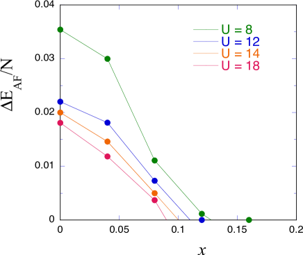
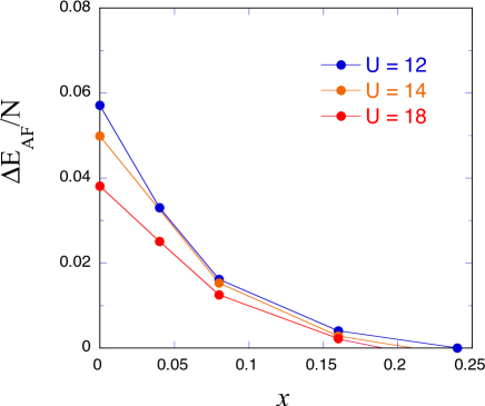
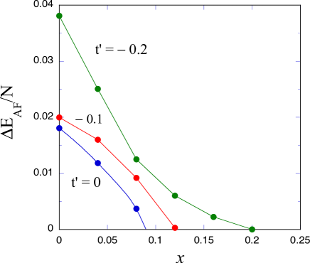
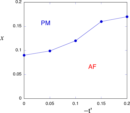
We show the condensation energy due to the AF magnetic order as a function of in Fig. 2 for . When is as large as , the AF region exists up to 10 doping. When , the AF region expands up to about 20 doping where even for large . We show this in Fig. 3. The AF region becomes larger as increases. Figure 4 shows as a function of for , , and , where we use . We show the AF region on the plane in Fig. 5. The AF state dominates near half-filling and is stabilized as increases. The -wave SC state exists near the boundary in Fig. 5.
4 Phase Separation
We discuss the phase separation in the 2D Hubbard model in this section. The existence of phase separation near half-filling in the 2D Hubbard model has been discussed[77, 78, 79]. This is a subject concerning the AF correlation and charge distribution in the case of small doped carriers. When there is a strong AF correlation between neighboring electrons, there may be a tendency that doped holes form clusters due to an effective attractive interaction between electrons. This means the possibility of phase separation with clusters of holes, depending on the AF correlation, attractive interaction, and kinetic energy gain. This is similar to the instability in the t-J model[80].
We examine an instability toward phase separation by evaluating the charge susceptibility
| (12) |
where is the ground-state energy and is the number of electrons. This is proportional to the second derivative of the energy with respect to the electron number. The negative sign of indicates an instability toward the phase separation. This instability is very subtle. Once the phase separation occurs, the ground state becomes an insulating state.
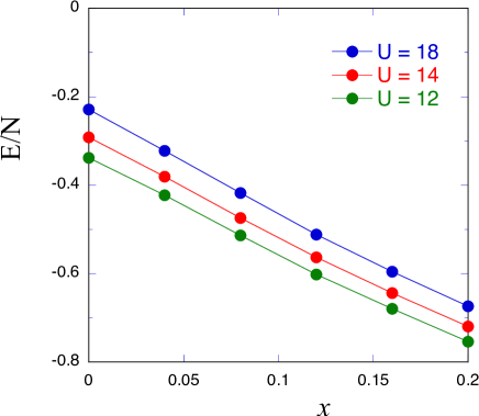
We show the energy as a function of the doping rate for in Fig. 6. The curve of the energy is usually convex downward, that is, , but the sign of changes in the region near half-filling. We show
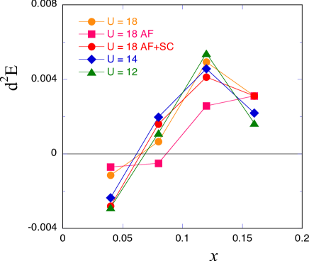
| (13) |
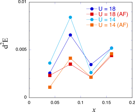
for in Fig. 7. This indicates that there is an instability toward the phase separation when for and . This is similar for and 12. When is nonzero and negative, the instability toward the phase separation occurs for a smaller doping rate. We show for in Fig. 8. In this case, for at least . The phase separation area decreases for .
Figure 8 indicates that shows a depression near for . This suggests the existence of strong charge fluctuation. We expect that this shows an instability toward some charge-ordered state such as the striped state.
In our optimized wave function, the instability toward the phase separation is limited to the range for and the region of phase separation becomes small for negative . We also mention that there is a possibility that the phase separation area will decrease as the wave function is optimized further by multiplying by operators and .
5 Superconducting phase
Let us now discuss the SC state. We evaluate the SC condensation energy defined by
| (14) |
where is the SC order parameter and is its optimized value. is the energy lowering due to the inclusion of the SC order parameter. We show the -dependence of in Fig. 9 on a lattice for and , where the upper curve is for the BCS-Gutzwiller function and the lower one is for the function. Both curves in Fig. 9 have a maximum at . This shows that high-temperature superconductivity is possible in the strongly correlated region.
We discuss here the coexistence of SC and AF phases in the range of . The wave function is written in the form
| (15) |
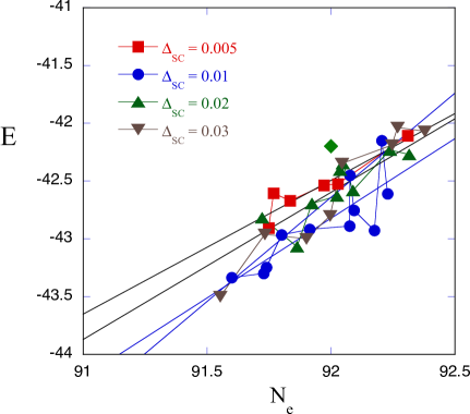
The BCS wave function with both the SC order parameter and the AF order parameter is formulated by solving the Bogoliubov equation[42, 12]. We show the ground-state energy as a function of the electron number near for in Fig. 10 for , 0.01, 0.02, and 0.03, where the chemical potential in the BCS wave function is changed to adjust the number of electrons. The energy is lowered slightly by introducing , by about per site at . Here we used the parameters , , and .
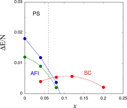
The condensation energy per site as a function of the hole density (doping rate) is shown in Fig. 11 for and on a lattice. There is an instability toward the phase separation for . Thus, the AF state for is an AF insulator. There is a coexistent metallic phase of superconductivity and antiferromagnetism when the doping rate is . The SC condensation energy at is that for the coexistent state. In the range , the pure -wave SC state exists. We have also presented the result obtained by using the level-4 function with the AF order parameter in Fig. 11:
| (16) |
where , , , and are variational parameters. The condensation energy of the AF state for is less than that for .
With the inclusion of , the phase separation region will decrease, and at the same time the area of the AF metallic state will increase. The phase diagram is dependent on .
6 Summary
We have investigated the ground-state properties of the 2D Hubbard model by using the optimization variational Monte Carlo method. We used the exponential-type wave function given in the form with an appropriate operator and a variational parameter . With our wave function, the ground-state energy is lowered greatly and the energy expectation value is lower than that obtained by any other wave functions such as the Gutzwiller wave function and also several proposed wave functions with many variational parameters. The ground-state energy is lowered by the kinetic-energy gain originating from .
The AF state is very stable near half-filling (with no carriers) in the 2D Hubbard model. The AF correlation is suppressed as the doping rate of holes increases. As the strength of the on-site Coulomb interaction increases, a crossover occurs between weakly correlated region and strongly correlated region. In the strongly correlated region, where is larger than , which is of the order of the bandwidth, the AF correlation is suppressed. A decrease in the AF correlation indicates an increase in spin and charge fluctuation. This fluctuation is caused by an increase in kinetic energy and is likely induce electron pairing. We expect that this is an origin of high-temperature superconductivity.
We have shown the phase diagram in the plane of (condensation energy) and the hole doping rate for . The value is most favorable for superconductivity, and for nonzero the AF area increases. In the underdoped region, where the doping rate is approximately , AF order and superconductivity coexist.
We have also discussed the instability toward the phase separation in the low-doping region. The occurrence of this instability is dependent on the balance between the kinetic energy gain of holes and the electron interaction between the adjacent lattices such as the pairing interaction and the AF interaction. In the range , the state of phase separation is realized for . In this region the AF state is an insulator, and becomes a metal when increases. The phase separation area decreases as increases. The region where AF and SC phases coexist becomes larger at the same time with increasing . We have also pointed out the depression in near for negative such as .
This work was supported by a Grant-in-Aid for Scientific Research from the Ministry of Education, Culture, Sports, Science and Technology of Japan (Grant No. 17K05559). The author expresses his sincere thanks to K. Yamaji and I. Hase for useful discussions. Part of the computations were supported by the Supercomputer Center of the Institute for Solid State Physics, the University of Tokyo.
References
- [1] J. G. Bednorz and K. A. Müller, Z. Phys. B 64, 189 (1986).
- [2] V. J. Emery, Phys. Rev. Lett. 58, 2794 (1987).
- [3] J. E. Hirsch, E. Y. Loh, D. J. Scalapino, and S. Tang, Phys. Rev. B 39, 243 (1989).
- [4] R. T. Scalettar, D. J. Scalapino, R. L. Sugar, and S. R. White, Phys. Rev. B 44, 770 (1991).
- [5] A. Oguri, T. Asahata, and S. Maekawa, Phys. Rev. B 49, 6880 (1994).
- [6] S. Koikegami and K. Yamada, J. Phys. Soc. Jpn. 69, 768 (2000).
- [7] T. Yanagisawa, S. Koike and K. Yamaji, Phys. Rev. Bi 64, 184509 (2001).
- [8] S. Koikegami and T. Yanagisawa, J. Phys. Soc. Jpn. 70, 3499 (2001).
- [9] T. Yanagisawa, S. Koike and K. Yamaji, Phys. Rev. B 67, 132408 (2003).
- [10] S. Koikegami and T. Yanagisawa, Phys. Rev. B 67, 134517 (2003).
- [11] S. Koikegami and T. Yanagisawa, J. Phys. Soc. Jpn. 75, 034715 (2006).
- [12] T. Yanagisawa, M. Miyazaki and K. Yamaji, J. Phys. Soc. Jpn. 78, 013706 (2009).
- [13] C. Weber, A. Lauchi, F. Mila and T. Giamarchi, Phys. Rev. Lett. 102, 017005 (2009).
- [14] B. Lau, M. Berciu and G. A. Sawatzky, Phys. Rev. Lett. 106, 036401 (2011).
- [15] C. Weber, T. Giamarchi and C. M. Varma, Phys. Rev. Lett. 112, 117001 (2014).
- [16] A. Avella, F. Mancini, F. Paolo and E. Plekhanov, Euro. Phys. J. B 86, 265 (2013).
- [17] H. Ebrahimnejad, G. A. Sawatzky and M. Berciu, J. Phys. Cond. Matter 28, 105603 (2016).
- [18] S. Tamura and H. Yokoyama, Phys. Procedia 81, 5 (2016).
- [19] C. Weber, K. Haule, and G. Kotliar, Phys. Rev. B 78, 134519 (2008).
- [20] M. S. Hybertsen, M. Schluter, and N. E. Christensen, Phys. Rev. B 39, 9028 (1989).
- [21] H. Eskes, G. A. Sawatzky, and L. F. Feiner, Physica C 160, 424 (1989).
- [22] A. K. McMahan, J. F. Annett, and R. M. Martin, Phys. Rev. B 42, 6268 (1990).
- [23] H. Eskes and G. Sawatzky, Phys. Rev. B 43, 119 (1991).
- [24] I. Hase and T. Yanagisawa, J. Phys. Soc. Jpn. 78, 084724 (2009).
- [25] J. Hubbard, Proc. R. Soc. London 276, 238 (1963).
- [26] J. Hubbard, Proc. R. Soc. London 281, 401 (1963).
- [27] M. C. Gutzwiller, Phys. Rev. Lett. 10, 159 (1963).
- [28] S. Zhang, J. Carlson and J. E. Gubernatis, Phys. Rev. B 55, 7464 (1997).
- [29] S. Zhang, J. Carlson and J. E. Gubernatis, Phys. Rev. Lett. 78, 4486 (1997).
- [30] T. Yanagisawa and Y. Shimoi, Int. J. Mod. Phys. B 10, 3383 (1996).
- [31] T. Yanagisawa and Y. Shimoi, Phys. Rev. Lett. 74, 4939 (1995).
- [32] T. Nakanishi, K. Yamaji and T. Yanagisawa, J. Phys. Soc. Jpn. 66, 294 (1997).
- [33] K. Yamaji, T. Yanagisawa, T. Nakanishi and S. Koike, Physica C 304, 225 (1998).
- [34] K. Yamaji, T. Yanagisawa and S. Koike, Physica B 284-288, 415 (2000).
- [35] K. Yamaji, T. Yanagisawa, M. Miyazaki, and R. Kadono, J. Phys. Soc. Jpn. 80, 083702 (2011).
- [36] T. M. Hardy, P. Hague, J. H. Samson and A. S. Alexandrov, Phys. Rev. B 79, 212501 (2009).
- [37] T. Yanagisawa, M. Miyazaki and K. Yamaji, J. Mod. Phys. 4, 33 (2013).
- [38] N. Bulut, Adv. Phys. 51, 1587 (2002).
- [39] H. Yokoyama, Y. Tanaka, M. Ogata and H. Tsuchiura, J. Phys. Soc. Jpn. 73, 1119 (2004).
- [40] H. Yokoyama, M. Ogata and Y. Tanaka, J. Phys. Soc. Jpn. 75, 114706 (2006).
- [41] T. Aimi and M. Imada, J. Phys. Soc. Jpn. 76, 113708 (2007).
- [42] M. Miyazaki, T. Yanagisawa and K. Yamaji, J. Phys. Soc. Jpn. 73, 1643 (2004).
- [43] T. Yanagisawa, New J. Phys. 10, 023014 (2008).
- [44] T. Yanagisawa, New J. Phys. 15, 033012 (2013).
- [45] T. Yanagisawa, J. Phys. Soc. Jpn. 85, 114707 (2016).
- [46] R. M. Noack, S. R. White and D. J. Scalapino, EPL 30, 163 (1995).
- [47] R. M. Noack, N. Bulut, D. J. Scalapino and M. G. Zacher, Phys. Rev. B 56, 7162 (1997).
- [48] K. Yamaji, Y. Shimoi and T. Yanagisawa, Physica C 235, 2221 (1994).
- [49] S. Koike, K. Yamaji, and T. Yanagisawa, J. Phys. Soc. Jpn. 68, 1657 (1999).
- [50] T. Yanagisawa, Y. Shimoi and K. Yamaji, Phys. Rev. B 52, R3860 (1995).
- [51] T. Nakano, K. Kuroki and S. Onari, Phys. Rev. B 76, 014515 (2007).
- [52] N. F. Mott, Metal-Insulator Transitions (Taylor and Francis, London, 1974).
- [53] T. Moriya, Spin Fluctuations in Itinerant Electron Magnetism (Springer, Berlin, 1985).
- [54] K. Yosida, Theory of Magnetism (Springer, Berlin, 1996).
- [55] J. Tranquada, J. D. Axe, N. Ichikawa, Y. Nakamura, S. Uchida, and B. Nachumi, Phys. Rev. B 54, 7489 (1996).
- [56] T. Suzuki, T. Goto, K. Chiba, T. Shinoda, T. Fukase, H. Kimura, K. Yamada, M. Ohashi, and Y. Yamaguchi, Phys. Rev. B 57, R3229(R) (1998).
- [57] K. Yamada, C. H. Lee, K. Kurahashi, J. Wada, S. Wakimoto, S. Ueki, H. Kimura, Y. Endoh, S. Hosoya, G. Shirane, R. J. Birgeneau, M. Greven, M. A. Kastner, and Y. J. Kim, Phys. Rev. B 57, 6165 (1998).
- [58] M. Arai, T. Nishijima, Y. Endoh, T. Egami, S. Tajima, K. Tomimoto, Y. Shiohara, M. Takahashi, A. Garrett, and S. M. Bennington, Phys. Rev. Lett. 83, 608 (1999).
- [59] H. A. Mook, P. Dai, F. Dogan, and R. D. Hunt, Nature 404, 729 (2000).
- [60] S. Wakimoto, R. J. Birgeneau, M. A. Kastner, Y. S. Lee, R. Erwin, P. M. Gehring, S. H. Lee, M. Fujita, K. Yamada, Y. Endoh, K. Hirota, and G. Shirane, Phys. Rev. B 61, 3699 (2000).
- [61] A. Bianconi, N. L. Saini, A. Lanzara, M. Missori, T. Rossetti, H. Oyanagi, H. Yamaguchi, K. Oka, and T. Ito, Phys. Rev. Lett. 76, 3412 (1996).
- [62] A. Bianconi, Nat. Phys. 9, 536 (2013).
- [63] J. E. Hoffman, E. W. hudson, K. M. Lang, V. Madhavan, H. Eisaki, S. Uchida, and J. C. Davis, Science 295, 466 (2002).
- [64] W. D. Wise, M. C. Boyer, K. Chatterjee, T. Kondo, T. Takeuchi, H. Ikuta, Y. Wang, and E. W. Hudson, Nat. Phys. 4, 696 (2008).
- [65] T. Hanaguri, C. Lupien, Y. Kohsaka, D.-H. Lee, M. Azuma, M. Takano, H. Takagi, and J. C. Davis, Nature 430, 1001 (2004).
- [66] M. Miyazaki, T. Yanagisawa, K. Yamaji and R. Kadono, J. Phys, Soc. Jpn. 78, 043706 (2009).
- [67] T. Yanagisawa, S. Koike and K. Yamaji, J. Phys. Soc. Jpn. 67, 3867 (1998).
- [68] H. Otsuka, J. Phys. Soc. Jpn. 61, 1645 (1992).
- [69] T. Yanagisawa, S. Koike and K. Yamaji, J. Phys. Soc. Jpn. 68, 3608 (1999).
- [70] D. Eichenberger and D. Baeriswyl, Phys. Rev. B 76, 180504 (2007).
- [71] D. Baeriswyl, D. Eichenberger and M. Menteshashvii, New J. Phys. 11, 075010 (2009).
- [72] D. Baeriswyl, J. Supercond. Novel Magn. 24, 1157 (2011).
- [73] T. Yanagisawa and M. Miyazaki, EPL 107, 27004 (2014).
- [74] T. Yanagisawa, Phys. Rev. B 75, 224503 (2007).
- [75] T. Misawa and M. Imada, Phys. Rev. B 90, 115137 (2014).
- [76] R. Sato and H. Yokoyama, J. Phys. Soc. Jpn. 85, 074701 (2016).
- [77] A. N. Andriotis, E. N. Economou, Q. Li, C. M. Soukoulis, Phys. Rev. B 47, 9208 (1993).
- [78] A. C. Cosentini, M. Capone, L. Guidoni, G. B. Bachelet, Phys. Rev. B 58, R14685(R) (1998).
- [79] A. Macridin, M. Jarrell, Th. Maier, Phys. Rev. B 74, 085104 (2006).
- [80] R. Sato and H. Yokoyama, J. Phys. Soc. Jpn. 87, 114003 (2018).