Unsupervised Speech Enhancement Based on
Multichannel NMF-Informed Beamforming
for Noise-Robust Automatic Speech Recognition

Abstract

This paper describes multichannel speech enhancement for improving automatic speech recognition (ASR) in noisy environments. Recently, the minimum variance distortionless response (MVDR) beamforming has widely been used because it works well if the steering vector of speech and the spatial covariance matrix (SCM) of noise are given. To estimating such spatial information, conventional studies take a supervised approach that classifies each time-frequency (TF) bin into noise or speech by training a deep neural network (DNN). The performance of ASR, however, is degraded in an unknown noisy environment. To solve this problem, we take an unsupervised approach that decomposes each TF bin into the sum of speech and noise by using multichannel nonnegative matrix factorization (MNMF). This enables us to accurately estimate the SCMs of speech and noise not from observed noisy mixtures but from separated speech and noise components. In this paper we propose online MVDR beamforming by effectively initializing and incrementally updating the parameters of MNMF. Another main contribution is to comprehensively investigate the performances of ASR obtained by various types of spatial filters, i.e., time-invariant and variant versions of MVDR beamformers and those of rank-1 and full-rank multichannel Wiener filters, in combination with MNMF. The experimental results showed that the proposed method outperformed the state-of-the-art DNN-based beamforming method in unknown environments that did not match training data.

I Introduction

Multichannel speech enhancement using a microphone array plays a vital role for distant automatic speech recognition (ASR) in noisy environments. A standard approach to multichannel speech enhancement is to use beamforming [1, 2, 3, 4, 5, 6, 7, 8, 9, 10]. Given the spatial information of speech and noise, we can emphasize the speech coming from one direction and suppress the noise from the other directions [11, 12, 13, 14, 15]. This approach was empirically shown to achieve the significant improvement of ASR performance in the CHiME Challenge [16, 17, 18]. There are many variants of beamforming such as multichannel Wiener filtering (MWF) [11, 12], minimum variance distortionless response (MVDR) beamforming [13], generalized sidelobe cancelling (GSC) [14], and generalized eigenvalue (GEV) beamforming [15], which are all performed in the time-frequency (TF) domain.

To calculate demixing filters for beamforming, the steering vector of speech and the spatial covariance matrix (SCM) of noise should be estimated. The steered response power phase transform (SRP-PHAT) [19] and the weighted delay-and-sum (DS) beamforming [20] are not sufficiently robust to real environments [16]. Recently, estimation of TF masks has actively been investigated [1, 2, 3, 4, 5, 6, 7, 8], assuming that each TF bin of an observed noisy speech spectrogram is classified into speech or noise. The SCMs of speech and noise are then calculated from the classified TF bins. The steering vector of the target speech is obtained as the principal component of the SCM of the speech [1, 3, 2]. For such binary classification, an unsupervised method based on complex Gaussian mixture models (CGMMs) [1] and a supervised method based on deep neural networks (DNNs) [3, 4, 2, 7, 8, 5, 6] have been proposed.

Although DNN-based beamforming works well in controlled experimental environments, it has two major problems in real environments. One problem is that the performance of ASR in unknown environments is often be considerably degraded due to the overfitting to training data consisting of many pairs of noisy speech spectrograms and ideal binary masks (IBMs) of speech. Although multi-condition training with various kinds of noisy environments mitigates the problem [21], it is still an open question whether DNN-based beamforming works when a microphone array with different geometry and frequency characteristics is used in unseen noisy environments. The other problem is that the spatial features such as inter-channel level and phase differences (ILDs and IPDs), which play an essential role in conventional multichannel audio signal processing, are simply input to DNNs without considering the physical meanings and generative processes of those features.

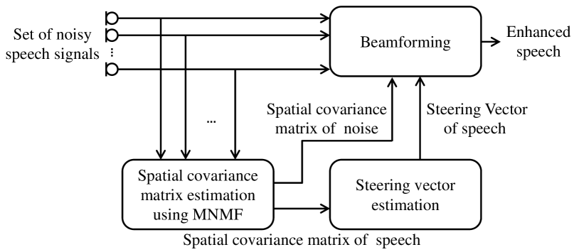
Figure 1: The proposed approach to unsupervised speech enhancement based on a variant of beamforming that calculates the SCMs of speech and noise from the corresponding spectrograms obtained by MNMF.

To solve these problems, we recently proposed an unsupervised method of speech enhancement [22] based on several types of beamforming using the SCMs of speech and noise estimated by a blind source separation (BSS) method called multichannel nonnegative matrix factorization (MNMF)[23] (Fig. 1). Given the multichannel complex spectrograms of mixture signals, MNMF can estimate the SCMs of multiple sources (i.e., speech and multiple noise sources) as well as represent the nonnegative power spectrogram of each source as the product of two nonnegative matrices corresponding to a set of basis spectra and a set of temporal activations. The SCMs of speech and noise estimated by MNMF that decomposes each TF bin into the sum of speech and noise are expected to be more accurate than those estimated by a CGMM[1] or a DNN[3, 4, 5, 6, 2, 7, 8] that classifies each TF bin into speech or noise. The unsupervised speech enhancement method is also expected to work well even in unknown environments for which there are no matched training data. In this paper, we newly propose an online extension of MNMF-informed beamforming that can process the observed mixture signals in a streaming manner.

The main contribution of this paper is to describe the complete formulation of the proposed method of MNMF-informed beamforming and report comprehensive comparative experiments. More specifically, we test the combination of MNMF with various types of beamforming, i.e., the time-variant and time-invariant versions of full-rank MWF [11], rank-1 MWF [12], and MVDR beamforming [13], using the CHiME-3 data and a real internal test set. These variants are compared with the state-of-the-art methods of DNN-based beamforming[3] using phase-aware acoustic features [4, 5, 6] and cost functions[24]. In addition, we evaluate the performance of the online extension of the proposed method.

The rest of this paper is organized as follows. Section II describes related work on multichannel speech enhancement. Section III and Section IV explain three types of beamforming (full-rank MWF, rank-1 MWF, and MVDR beamforming) and MNMF, respectively. Section V explains the proposed method of MNMF-informed beamforming. Section VI reports comparative experiments and Section VII concludes the paper.

II Related Work

We review non-blind beamforming methods based on the steering vector of speech and the SCM of noise for ASR in noisy environments. We also review BSS methods including several variants of MNMF.

II-A Beamforming Methods

There are several variants of beamforming such as DS [20] MVDR [13], GEV [15] beamforming and MWF [11, 12]. The DS beamforming [20] uses only the steering vector of target speech and the other methods additionally use the SCM of noise. The GEV beamforming aims to maximize the signal-to-noise ratio (SNR) [15] without putting any assumptions on the acoustic transfer function from the speaker to the array and the SCM of the noise. The MVDR beamforming and the MWF, on the other hand, assume that the time-frequency (TF) bins of speech and noise spectrograms are distributed according to complex Gaussian distributions [13, 11, 12]. In Section III, we review the relationships between MVDR beamforming and rank-1 and full-rank MWF in terms of the propagation process and and the filter estimation strategy.

TF Mask estimation has actively been studied for computing the SCMs of speech and noise [1, 2, 3, 4, 7, 8, 5, 6]. Our unsupervised method is different from DNN-based mask estimation [2, 3, 4, 7, 8, 5, 6] in two ways. First, our method decomposes each TF bin into the sum of speech and noise, while the mask-based methods calculate the SCM of speech from noisy TF bins without any decomposition. Second, our method uses no training data, while in general the DNN-based methods need a sufficient number of pairs of noisy spectrograms and ideal binary masks (IBMs). The performance of the DNN-based mask estimation would be degraded in unseen conditions that are not covered by the training data because of overfitting to the training data.

The major limitation of most DNN-based methods is that only single-channel magnitude spectrograms are used for mask estimation by discarding the spatial information such as ILDs and IPDs. Recently, Wang et al.[6] and Pertilä[5] have investigated the use of ILDs and IPDs as acoustic features for mask estimation. Erdogan et al.[24] proposed a method for estimating a phase-sensitive filter in single-channel speech enhancement. For comparative evaluation, inspired by these state-of-the-art methods, we use both spatial and magnitude features for DNN-based multichannel mask estimation.

II-B Multichannel Nonnegative Matrix Factorization

Multichannel extensions of NMF [25, 26, 27, 23, 28, 29] represent the complex spectrograms of multichannel mixture signals by using the SCMs and low-rank power spectrograms of multiple source signals. Ozerov et al. [26] pioneered the use of NMF for multichannel source separation, where the SCMs are restricted to rank-1 matrices and the cost function based on the Itakura-Saito (IS) divergence is minimized. This model was extended to have full-rank SCMs [27]. Sawada et al. [23] introduced partitioning parameters to have a set of basis spectra shared by all sources and derived a majorization-minimization (MM) algorithm. Nikunen and Virtanen [28] proposed a similar model that represents the SCM of each source as the weighted sum of direction-dependent SCMs. While these methods can be used in a underdetermined case, Kitamura et al. [29] proposed independent low-rank matrix analysis (ILRMA) for a determined case by restricting the SCMs of [23] to rank-1 matrices. This can be viewed as a unified model of NMF and independent vector analysis (IVA) and is robust to initialization.

III Beamforming Methods

This section introduces three major methods of beamforming; full-rank and rank-1 versions of multichannel Wiener filtering (MWF) and minimum variance distortionless response (MVDR) beamforming (Table I)[11].

TABLE I: Beamforming methods.

	Speech: Full-rank	Speech: Rank-1
	Noise: Full-rank	Noise: Full-rank
MAP	Full-rank MWF	Rank-1 MWF
	Eqs. (8) & (9)	Eqs. (12) & (13)
ML	-	MVDR
	-	Eqs. (15) & (16)

III-A Overview

The goal of beamforming is to extract a source signal of interest from a mixture signal in the short-time Fourier transform (STFT) domain. Let $\mathbf{x}_{ft}\in{\mathbb{C}}^{M}$ be the multichannel complex spectrum of the mixture at frequency $f$ and frame $t$ recorded by $M$ microphones, which is assumed to be given by

$$\mathbf{x}_{ft}=\mathbf{x}^{\mathrm{s}}_{ft}+\mathbf{x}^{\mathrm{n}}_{ft},$$ (1)

where $\mathbf{x}^{\mathrm{s}}_{ft}$ and $\mathbf{x}^{\mathrm{n}}_{ft}$ are the multichannel complex spectra of speech and noise (called images), respectively. The notations are listed in Table II. The goal is to estimate a linear demixing filter $\mathbf{w}_{ft}$ that obtains an estimate $\hat{s}_{ft}$ of the target speech $s_{ft}$ from the mixture (speech + noise) $\mathbf{x}_{ft}$ as follows:

$$\hat{s}_{ft}=\mathbf{w}_{ft}^{\mathrm{H}}\mathbf{x}_{ft}.$$ (2)

As shown in Table I, the beamforming methods can be categorized in terms of sound propagation processes.

• The full-rank propagation process considers various propagation paths caused by reflection and reverberation. It is thus represented by using an $M\times M$ full-rank SCM for each source.

• The rank-1 propagation process considers only the direct paths from each sound source to the microphones. It is thus represented by using an $M$-dimensional steering vector for each source.

The full-rank propagation process reduces to the rank-1 propagation process when the full-rank SCM is restricted to a rank-1 matrix whose eigenvector is equal to the steering vector.

The beamforming methods can also be categorized in terms of estimation strategies.

• The maximum a posteriori (MAP) estimation assumes the target speech spectra to be complex Gaussian distributed.

• The maximum likelihood (ML) estimation uses no prior knowledge about the target speech spectra.

TABLE II: Mathematical notations.

	Observation	Speech	Noise
Multichannel spectrum $\in\mathbb{C}^{M}$	$\mathbf{x}$	$\mathbf{x}^{\mathrm{s}}$	$\mathbf{x}^{\mathrm{n}}$
Steering vector $\in\mathbb{C}^{M}$	-	$\mathbf{p}$	$\mathbf{q}$
Spatial covariance matrix $\in\mathbb{S}_{++}^{M}$	$\mathbf{X}$	$\mathbf{P}$	$\mathbf{Q}$

III-B Full-Rank Multichannel Wiener Filtering

The full-rank MWF [30] assumes both the target speech $\mathbf{x}^{\mathrm{s}}_{ft}$ and the noise $\mathbf{x}^{\mathrm{n}}_{ft}$ to follow multivariate circularly-symmetric complex Gaussian distributions as follows:

$$\mathbf{x}^{\mathrm{s}}_{ft} \sim\mathcal{N}_{\mathbb{C}}(\mathbf{0},\mathbf{P}_{ft}),$$ (3)

$$\mathbf{x}^{\mathrm{n}}_{ft} \sim\mathcal{N}_{\mathbb{C}}(\mathbf{0},\mathbf{Q}_{ft}),$$ (4)

where $\mathbf{P}_{ft}\in\mathbb{S}_{++}^{M}$ and $\mathbf{Q}_{ft}\in\mathbb{S}_{++}^{M}$ are the full-rank SCMs of the speech and noise at frequency $f$ and time $t$, respectively, and $\mathbb{S}_{++}^{M}$ indicates the set of $M\times M$ Hermitian positive definite matrices. Using the reproducible property of the Gaussian distribution, we have

$$\mathbf{x}_{ft} \sim\mathcal{N}_{\mathbb{C}}(\mathbf{0},\mathbf{P}_{ft}+\mathbf{Q}_{ft}){\color[rgb]{1,0,0}.}$$ (5)

Given the mixture $\mathbf{x}_{ft}$, the posterior distribution of the multichannel speech image $\mathbf{x}^{\mathrm{s}}_{ft}$ is obtained as follows:

$$\mathbf{x}^{\mathrm{s}}_{ft}\mid\mathbf{x}_{ft} \sim\mathcal{N}_{\mathbb{C}}\!\left(\mathbf{P}_{ft}\left(\mathbf{P}_{ft}+\mathbf{Q}_{ft}\right)^{-1}\mathbf{x}_{ft},\right.$$ (6)

$$\ \ \ \ \ \ \ \ \ \left.\mathbf{P}_{ft}-\mathbf{P}_{ft}\left(\mathbf{P}_{ft}+\mathbf{Q}_{ft}\right)^{-1}\mathbf{P}_{ft}\right).$$ (7)

To obtain a monaural estimate $\hat{s}_{ft}$ of the speech, it is necessary to choose a reference channel (dimension) $m$ from the MAP estimate of the speech image $\mathbf{x}^{\mathrm{s}}_{ft}$. The time-variant demixing filter $\mathbf{w}_{ft}^{\mbox{\tiny WF}}$ is thus given by

$$\mathbf{w}_{ft}^{\mbox{\tiny WF}}(m)=({\mathbf{P}_{ft}}+{\mathbf{Q}_{ft}})^{-1}{\mathbf{P}_{ft}}\mathbf{u}_{m},$$ (8)

where $\mathbf{u}_{m}\in{\mathbb{C}}^{M}$ is the $M$-dimensional one-hot vector that takes $1$ in dimension $m$. If the speaker does not move and the noise is stationary, $\mathbf{P}_{ft}$ and $\mathbf{Q}_{ft}$ are often assumed to be time-invariant, i.e., $\mathbf{P}_{ft}=\mathbf{P}_{f}$ and $\mathbf{Q}_{ft}=\mathbf{Q}_{f}$. In this case, the time-invariant demixing filter $\mathbf{w}_{f}^{\mbox{\tiny WF}}$ is given by

$$\mathbf{w}_{f}^{\mbox{\tiny WF}}(m)=({\mathbf{P}_{f}}+{\mathbf{Q}_{f}})^{-1}{\mathbf{P}_{f}}\mathbf{u}_{m}.$$ (9)

In reality, the speech is not stationary, but such time-invariant linear filtering is known to be effective for speech enhancement with small distortion. In general, the enhanced speech signals obtained by the time-variant filter tends to be more distorted than those obtained by the time-invariant filter.

The optimal reference channel $m^{*}$ is chosen such that the average-a-posteriori SNR is maximized with respect to $m$ as follows [4, 31]:

$$m^{*}=\mathop{\rm argmax}_{m}\frac{\sum_{t=1}^{T}\sum_{f=1}^{F}\mathbf{w}_{ft}^{\mathrm{H}}(m)\mathbf{P}_{ft}\mathbf{w}_{ft}(m)}{\sum_{t=1}^{T}\sum_{f=1}^{F}\mathbf{w}_{ft}^{\mathrm{H}}(m)\mathbf{Q}_{ft}\mathbf{w}_{ft}(m)},$$ (10)

where $\mathbf{w}_{ft}(m)$ is a demixing filter obtained by assuming the reference channel to be $m$. Different microphones may thus be selected for individual utterances.

III-C Rank-1 Multichannel Wiener Filtering

The rank-1 MWF [32] is obtained as a special case of the full-rank MWF when the spatial covariance matrix $\mathbf{P}_{ft}$ of the speech is restricted to a rank-1 matrix as follows:

$$\mathbf{P}_{ft}=\lambda_{ft}\mathbf{p}_{ft}\mathbf{p}_{ft}^{\mathrm{H}},$$ (11)

where $\lambda_{ft}$ and $\mathbf{p}_{ft}\in\mathbb{C}^{M}$ are the power and steering vector of the speech at frequency $f$ and time $t$, respectively. Substituting Eq. (11) into Eq. (8) and using the Woodbury matrix identity, we obtain the time-variant demixing filter $\mathbf{w}_{ft}^{\mbox{\tiny WF1}}$ as follows:

$$\mathbf{w}_{ft}^{\mbox{\tiny WF1}}(m)=\frac{\mathbf{Q}_{ft}^{-1}\mathbf{p}_{ft}}{\mathbf{p}_{ft}^{\mathrm{H}}\mathbf{Q}_{ft}^{-1}\mathbf{p}_{ft}+\lambda_{ft}^{-1}}\mathbf{p}_{ft}^{\mathrm{H}}\mathbf{u}_{m}.$$ (12)

In practice, to achieve reasonable performance, we assume the time-invariance of the speech, i.e., $\lambda_{ft}=\lambda_{f}$ and $\mathbf{p}_{ft}=\mathbf{p}_{f}$. Similarly, the time-invariant filter $\mathbf{w}_{f}^{\mbox{\tiny WF1}}$ is given by

$$\mathbf{w}_{f}^{\mbox{\tiny WF1}}(m)=\frac{\mathbf{Q}_{f}^{-1}\mathbf{p}_{f}}{\mathbf{p}_{f}^{\mathrm{H}}\mathbf{Q}_{f}^{-1}\mathbf{p}_{f}+\lambda_{f}^{-1}}\mathbf{p}_{f}^{\mathrm{H}}\mathbf{u}_{m}.$$ (13)

Given the steering vector $\mathbf{p}_{ft}$ or $\mathbf{p}_{f}$, the power spectral density $\lambda_{ft}$ in Eqs. (12) or $\lambda_{f}$ in (13), can be estimated as follows:

$$\lambda_{ft}\simeq\frac{\|\mathbf{P}_{ft}\|}{\|\mathbf{p}_{ft}\mathbf{p}_{ft}^{\mathrm{H}}\|},\ \ \ \lambda_{f}\simeq\frac{\|\mathbf{P}_{f}\|}{\|\mathbf{p}_{f}\mathbf{p}_{f}^{\mathrm{H}}\|},$$ (14)

where $\|\cdot\|$ represents the Frobenius norm of a matrix.

III-D Minimum Variance Distortionless Response Beamforming

The MVDR beamforming [13] can be derived as a special case of the rank-1 MWF when the power spectral density of the speech in Eq. (11) (the variance of the Gaussian distribution in Eq. (3)) approaches infinity, i.e., we do not put any assumption on the target speech. The time-variant and time-invariant demixing filters are given by

$$\mathbf{w}_{ft}^{\mbox{\tiny MV}}(m) =\frac{\mathbf{Q}_{ft}^{-1}\mathbf{p}_{ft}}{\mathbf{p}_{ft}^{\mathrm{H}}\mathbf{Q}_{ft}^{-1}\mathbf{p}_{ft}}\mathbf{p}_{ft}^{\mathrm{H}}\mathbf{u}_{m},$$ (15)

$$\mathbf{w}_{f}^{\mbox{\tiny MV}}(m) =\frac{\mathbf{Q}_{f}^{-1}\mathbf{p}_{f}}{\mathbf{p}_{f}^{\mathrm{H}}\mathbf{Q}_{f}^{-1}\mathbf{p}_{f}}\mathbf{p}_{f}^{\mathrm{H}}\mathbf{u}_{m}.$$ (16)

IV Multichannel Nonnegative Matrix Factorization

This section introduces multichannel nonnegative matrix factorization (MNMF)[23]. In this paper we assume that the observed noisy speech contains $N$ sound sources, one of which corresponds to target speech and the other sources are regarded as noise. Let $M$ be the number of channels (microphones).

IV-A Probabilistic Formulation

We explain the generative process of the multichannel observations of noisy speech, $\mathbf{X}=\{\mathbf{x}_{ft}\}_{f=1,t=1}^{F,T}$, where $\mathbf{x}_{ft}\in\mathbb{C}^{M}$ is the multichannel complex spectrum of the mixture at frequency $f$ and time $t$. Let $s_{nft}\in\mathbb{C}$ be the single-channel complex spectrum of source $n$ at frequency $f$ and time $t$ and $\mathbf{x}_{nft}\in\mathbb{C}^{M}$ be the multichannel complex spectrum (image) of source $n$. If the sources do not move, we have

$$\mathbf{x}_{nft}=\mathbf{g}_{nf}s_{nft},$$ (17)

where $\mathbf{g}_{nf}\in{\mathbb{C}}^{M}$ is the time-invariant steering vector of source $n$ at frequency $f$. Here $s_{ft}$ is assumed to be circularly-symmetric complex Gaussian distributed as follows:

$$s_{nft}\sim\mathcal{N}_{\mathbb{C}}\!\left(0,\lambda_{nft}\right),$$ (18)

where $\lambda_{nft}\geq 0$ is the power spectral density of source $n$ at frequency $f$ and time $t$. Using Eq. (17) and Eq. (18), $\mathbf{x}_{nft}$ can be said to be multivariate circularly-symmetric complex Gaussian distributed as follows:

$$\mathbf{x}_{nft}\sim\mathcal{N}_{\mathbb{C}}\!\left(\mathbf{0},\lambda_{nft}\mathbf{G}_{nf}\right),$$ (19)

where and $\mathbf{G}_{nf}=\mathbf{g}_{nf}\mathbf{g}_{nf}^{\mathrm{H}}$ is the rank-1 SCM of source $n$ at frequency $f$. In MNMF, the rank-1 assumption on $\mathbf{G}_{nf}$ is relaxed to deal with the underdetermined condition of $M<N$ by allowing $\mathbf{G}_{nf}\in\mathbb{S}_{++}^{M}$ to take any full-rank positive definite matrix. Assuming the instantaneous mixing process (source additivity) in the frequency domain, we have

$$\mathbf{x}_{ft}=\sum_{n=1}^{N}\mathbf{x}_{nft}.$$ (20)

Using Eq. (19) and Eq. (20), the reproducible property of the Gaussian distribution leads to

$$\mathbf{x}_{ft}\sim\mathcal{N}_{\mathbb{C}}\!\left(\mathbf{0},\sum_{n=1}^{N}\lambda_{nft}\mathbf{G}_{nf}\right).$$ (21)

The nonnegative power spectral density $\lambda_{nft}$ of each source $n$ is assumed to be factorized in an NMF style as follows:

$$\lambda_{nft}=\sum_{k=1}^{K}v_{nkf}h_{nkt},$$ (22)

where $K$ is the number of basis spectra, $v_{nkf}\geq 0$ is the power of basis $k$ at frequency $f$ and $h_{nkt}\geq 0$ is the activation of basis $k$ at time $t$. This naive model has $NK$ basis spectra in total. One possibility to reduce the number of parameters is to share $K$ basis spectra between all $N$ sources as follows:

$$\lambda_{nft}=\sum_{k=1}^{K}z_{nk}v_{kf}h_{kt},$$ (23)

where $z_{nk}$ indicates the weight of basis $k$ in source $n$. Substituting Eq. (23) into Eq. (21), we obtain the probabilistic generative model of $\mathbf{X}$ as follows:

$$\mathbf{x}_{ft}\sim\mathcal{N}_{\mathbb{C}}\!\left(\mathbf{0},\sum_{k=1}^{K}v_{kf}h_{kt}\sum_{n=1}^{N}z_{nk}\mathbf{G}_{nf}\right).$$ (24)

IV-B Parameter Estimation

Given $\mathbf{X}$, our goal is to estimate $\mathbf{V}=\{v_{kf}\}_{k=1,f=1}^{K,F}$, $\mathbf{H}=\{h_{kt}\}_{k=1,t=1}^{K,T}$, $\mathbf{Z}=\{z_{nk}\}_{n=1,k=1}^{N,K}$, and $\mathbf{G}=\{\mathbf{G}_{nf}\}_{n=1,f=1}^{N,F}$ that maximize the likelihood obtained by multiplying Eq. (24) over all frequency $f$ and time $t$. Let two positive definite matrices $\mathbf{X}_{ft}\in\mathbb{S}_{++}^{M}$ and $\mathbf{Y}_{ft}\in\mathbb{S}_{++}^{M}$ be as follows:

$$\mathbf{X}_{ft} =\mathbf{x}_{ft}\mathbf{x}_{ft}^{\mathrm{H}},$$ (25)

$$\mathbf{Y}_{ft} =\sum_{k=1}^{K}v_{kf}h_{kt}\sum_{n=1}^{N}z_{nk}\mathbf{G}_{nf}.$$ (26)

The maximization of the likelihood function given by Eq. (24) is equivalent to the minimization of the log-determinant divergence between $\mathbf{X}_{ft}$ and $\mathbf{Y}_{ft}$ given by

$$\!\!\!\mathcal{D}_{\mbox{\scriptsize LD}}(\mathbf{X}_{ft}|\mathbf{Y}_{ft})=\mbox{tr}\!\left(\mathbf{X}_{ft}\mathbf{Y}_{ft}^{-1}\right)-\log\!\left|\mathbf{X}_{ft}\mathbf{Y}_{ft}^{-1}\right|-M,$$ (27)

The total cost function $f(\mathbf{V},\mathbf{H},\mathbf{Z},\mathbf{G})$ to be minimized w.r.t. $\mathbf{V}$, $\mathbf{H}$, $\mathbf{Z}$, and $\mathbf{G}$ is thus given by

$$f(\mathbf{V},\mathbf{H},\mathbf{Z},\mathbf{G})=\sum_{f=1}^{F}\sum_{t=1}^{T}\mathcal{D}_{\mbox{\scriptsize LD}}(\mathbf{X}_{ft}|\mathbf{Y}_{ft}).$$ (28)

Since Eq. (28) is hard to directly minimize, a convergence-guaranteed MM algorithm was proposed (see [23] for detailed derivation). The updating rules are given by

$$v_{kf} \leftarrow v_{kf}\sqrt{\frac{\sum_{n}{z}_{nk}\sum_{t}h_{kt}{\rm tr}\!\left(\mathbf{Y}_{ft}^{-1}\mathbf{X}_{ft}\mathbf{Y}_{ft}^{-1}\mathbf{G}_{nf}\right)}{\sum_{n}{z}_{nk}\sum_{t}h_{kt}{\rm tr}\!\left(\mathbf{Y}_{ft}^{-1}\mathbf{G}_{nf}\right)}},$$ (29)

$$h_{kt} \leftarrow h_{kt}\sqrt{\frac{\sum_{n}{z}_{nk}\sum_{f}v_{kf}{\rm tr}\!\left(\mathbf{Y}_{ft}^{-1}\mathbf{X}_{ft}\mathbf{Y}_{ft}^{-1}\mathbf{G}_{nf}\right)}{\sum_{n}{z}_{nk}\sum_{f}v_{kf}{\rm tr}\!\left(\mathbf{Y}_{ft}^{-1}\mathbf{G}_{nf}\right)}},$$ (30)

$${z}_{nk} \leftarrow{z}_{nk}\sqrt{\frac{\sum_{f}v_{kf}\sum_{t}h_{kt}{\rm tr}\!\left(\mathbf{Y}_{ft}^{-1}\mathbf{X}_{ft}\mathbf{Y}_{ft}^{-1}\mathbf{G}_{nf}\right)}{\sum_{f}v_{kf}\sum_{t}h_{kt}{\rm tr}\!\left(\mathbf{Y}_{ft}^{-1}\mathbf{G}_{nf}\right)}}.$$ (31)

$\mathbf{G}_{nf}$ is obtained as the unique solution of a special case of the continuous time algebraic Riccati equation $\mathbf{G}_{nf}\bm{\Psi}_{nf}\mathbf{G}_{nf}=\mathbf{G}_{nf}^{\mbox{\scriptsize old}}\bm{\Phi}_{nf}\mathbf{G}_{nf}^{\mbox{\scriptsize old}}$. In the original study on MNMF [23], this equation was solved using an iterative optimization algorithm. In the field of information geometry, however, the analytical solution of this equation is known to exist as follows:

$$\bm{\Phi}_{nf} =\sum_{k}{z}_{nk}v_{kf}\sum_{t}h_{kt}\mathbf{Y}_{ft}^{-1}\mathbf{X}_{ft}\mathbf{Y}_{ft}^{-1},$$ (32)

$$\bm{\Psi}_{nf} =\sum_{k}{z}_{nk}v_{kf}\sum_{t}h_{kt}\mathbf{Y}_{ft}^{-1},$$ (33)

$$\mathbf{G}_{nf} \leftarrow\bm{\Psi}_{nf}^{-\frac{1}{2}}\left(\bm{\Psi}_{nf}^{\frac{1}{2}}\mathbf{G}_{nf}\bm{\Phi}_{nf}\mathbf{G}_{nf}\bm{\Psi}_{nf}^{\frac{1}{2}}\right)^{\frac{1}{2}}\bm{\Psi}_{nf}^{-\frac{1}{2}},$$ (34)

where $\mathbf{G}_{nf}$ is updated to the geometric mean of two positive definite matrices $\bm{\Psi}_{nf}^{-1}$ and $\mathbf{G}_{nf}^{\mbox{\scriptsize old}}\bm{\Phi}_{nf}\mathbf{G}_{nf}^{\mbox{\scriptsize old}}$ [33, 34, 35].

V MNMF-Informed Beamforming

This section explains the proposed MNMF-informed beamforming and its online extension. Our method takes as input the multichannel noisy speech spectrograms $\mathbf{X}$ and outputs a speech spectrogram, which is then passed to an ASR back-end (Fig. 1). MNMF is used to estimate the SCMs of speech and the other sounds from $\mathbf{X}$. The steering vector $\mathbf{p}$ of the target speech and the SCM $\mathbf{Q}$ of noise are then computed. Finally, the enhanced speech is obtained by using one of the three kinds of beamforming described in Section III.

V-A Estimation of Spatial Information

To use a beamforming method (Section III), we compute the SCMs $\mathbf{P}$ and $\mathbf{Q}$ of speech and noise by using the parameters $\mathbf{V}$, $\mathbf{H}$, $\mathbf{Z}$, and $\mathbf{G}$ of MNMF (Section IV). Assuming that source $n=1$ is the target speech (see Section V-C), we have

$$\mathbf{P}_{ft} =\sum_{k=1}^{K}v_{kf}h_{kt}z_{1k}\mathbf{G}_{f1},$$ (35)

$$\mathbf{Q}_{ft} =\sum_{k=1}^{K}v_{kf}h_{kt}\sum_{n=2}^{N}z_{nk}\mathbf{G}_{nf},$$ (36)

where $\mathbf{P}_{ft}$ and $\mathbf{Q}_{ft}$ are the time-variant SCMs of speech and noise, respectively. The time-invariant SCMs $\mathbf{P}_{f}$ and $\mathbf{Q}_{f}$ are also given by

$$\mathbf{P}_{f} =\frac{1}{T}\sum_{t=1}^{T}\mathbf{P}_{ft},$$ (37)

$$\mathbf{Q}_{f} =\frac{1}{T}\sum_{t=1}^{T}\mathbf{Q}_{ft}.$$ (38)

The corresponding steering vectors $\mathbf{p}_{ft}$ and $\mathbf{p}_{f}$ of the target speech are approximated as the principal components of $\mathbf{P}_{ft}$ and $\mathbf{P}_{f}$, respectively, as follows:

$$\mathbf{p}_{ft} =\mathcal{PE}\!\left(\mathbf{P}_{ft}\right),$$ (39)

$$\mathbf{p}_{f} =\mathcal{PE}\!\left(\mathbf{P}_{f}\right).$$ (40)

V-B Online MNMF

We propose an online extension of MNMF that incrementally updates the parameters $\mathbf{V}$, $\mathbf{H}$, $\mathbf{Z}$, and $\mathbf{G}$. Suppose that $\mathbf{X}$ is given as a series of $J$ mini-batches in a sequential order, where each mini-batch $j$ consists of multiple frames $\in{t}^{(j)}$. The notation $*^{(j)}$ represents a statistic of mini-batch $j$. The latest statistics are considered with a weight $\rho$. When $\rho<1$, the current mini-batch is put more emphasis [36]. The online updating rules are as follows:

$$\begin{split}{\alpha}_{kf}^{(j)}&={\sum_{n}{z}_{nk}^{(j)}\sum_{t\in{t}^{(j)}}h_{kt}{\rm tr}\!\left(\mathbf{Y}_{ft}^{-1}\mathbf{X}_{ft}\mathbf{Y}_{ft}^{-1}\mathbf{G}_{nf}^{(j)}\right)},\end{split}$$ (41)

$${\beta}_{kf}^{(j)} =\sum_{n}{z}_{nk}^{(j)}\sum_{t\in{t}^{(j)}}h_{kt}{\rm tr}\!\left(\mathbf{Y}_{ft}^{-1}\mathbf{G}_{nf}^{(j)}\right),$$ (42)

$$v_{kf}^{(j)} \leftarrow\sqrt{\frac{F_{j}(v_{kf},{\alpha}_{kf},v_{kf})}{F_{j}({\beta}_{kf})}},$$ (43)

$$\begin{split}{\gamma}_{nk}^{(j)}&={\sum_{f}v_{kf}^{(j)}\sum_{t\in{t}^{(j)}}h_{kt}{\rm tr}\!\left(\mathbf{Y}_{ft}^{-1}\mathbf{X}_{ft}\mathbf{Y}_{ft}^{-1}\mathbf{G}_{nf}^{(j)}\right)},\end{split}$$ (44)

$${\delta}_{nk}^{(j)} =\sum_{f}v_{kf}^{(j)}\sum_{t\in{t}^{(j)}}h_{kt}{\rm tr}\!\left(\mathbf{Y}_{ft}^{-1}\mathbf{G}_{nf}^{(j)}\right),$$ (45)

$${z}_{nk}^{(j)} \leftarrow\sqrt{\frac{F_{j}(z_{nk},{\gamma}_{nk},z_{nk})}{F_{j}({\delta}_{nk})}},$$ (46)

$$\begin{split}\bm{\Phi}_{nf}^{(j)}&=\sum_{k}{z}_{nk}^{(j)}v_{kf}^{(j)}\sum_{t\in{t}^{(j)}}h_{kt}\mathbf{Y}_{ft}^{-1}\mathbf{X}_{ft}\mathbf{Y}_{ft}^{-1},\end{split}$$ (47)

$$\bm{\Psi}_{nf}^{(j)} =\sum_{k}{z}_{nk}^{(j)}v_{kf}^{(j)}\sum_{t\in{t}^{(j)}}h_{kt}\mathbf{Y}_{ft}^{-1},$$ (48)

$$\mathbf{G}_{nf}^{(j)} \leftarrow F_{j}(\bm{\Psi}_{nf})^{-\frac{1}{2}}$$

$$\ \ \ \left(F_{j}^{\frac{1}{2}}(\bm{\Psi}_{nf})F_{j}(\mathbf{G}_{nf},\bm{\Phi}_{nf},\mathbf{G}_{nf})F_{j}^{\frac{1}{2}}(\bm{\Psi}_{nf})\right)^{\frac{1}{2}}$$

$$\ \ \ F_{j}(\bm{\Psi}_{nf})^{-\frac{1}{2}},$$ (49)

where the function $F_{j}$ is defined as follows:

$$F_{j}(x) =x^{(j)}+\rho x^{(j-1)},$$ (50)

$$F_{j}(a,x,a) =a^{(j)}x^{(j)}a^{(j)}+\rho a^{(j-1)}x^{(j-1)}a^{(j-1)}.$$ (51)

V-C Initialization of MNMF

We randomly initialize all parameters except for $\mathbf{G}$. Since MNMF is sensitive to the initialization of $\mathbf{G}$ [37], we use a constrained version of MNMF called independent low-rank matrix analysis (ILRMA) [29] for initializing $\mathbf{G}$. Since ILRMA can be used in the determined condition of $M=N$, in this paper we assume $M=N$ for MNMF. In ILRMA, $\mathbf{G}_{nf}$ is restricted to a rank-1 matrix, i.e., $\mathbf{G}_{nf}=\mathbf{g}_{nf}\mathbf{g}_{nf}$ (see Section IV-A). Using Eq. (17) and Eq. (20), we have

$$\mathbf{x}_{ft}=\mathbf{G}_{f}\mathbf{s}_{ft},$$ (52)

where $\mathbf{s}_{ft}=[s_{1ft},\cdots,s_{Nft}]^{\mathrm{T}}\in\mathbb{C}^{N}$ is a set of source spectra and $\mathbf{G}_{f}=[\mathbf{g}_{1f},\cdots,\mathbf{g}_{Nf}]\in\mathbb{C}^{M\times N}$ is a mixing matrix. If $\mathbf{G}_{f}$ is a non-singular matrix, we have

$$\mathbf{s}_{ft}=\mathbf{W}_{f}^{\mathrm{H}}\mathbf{x}_{ft},$$ (53)

where $\mathbf{W}_{f}^{\mathrm{H}}=[\mathbf{w}_{1f},\cdots,\mathbf{w}_{Nf}]^{\mathrm{H}}=\mathbf{G}_{f}^{-1}$ is a demixing matrix and $\mathbf{w}_{nf}\in\mathbb{C}^{M}$ is a demixing filter of source $n$. We use ILRMA for estimating $\mathbf{W}_{f}$, compute $\mathbf{G}_{f}=\mathbf{W}_{f}^{-\mathrm{H}}$, and initialize $\mathbf{G}_{nf}=\mathbf{g}_{nf}\mathbf{g}_{nf}+\epsilon\mathbf{I}$, where $\epsilon$ is a small number.

Algorithm 1 Offline MNMF-informed beamforming.

1:  Initialize $\mathbf{G}$ by ILRMA

2:  for iteration $=1$ to MaxIteration  do

3:     Update $\mathbf{V}$ by Eq. (29)

4:     Update $\mathbf{H}$ by Eq. (30)

5:     Update $\mathbf{Z}$ by Eq. (31)

6:     Update $\mathbf{G}$ by Eq. (34)

7:  end for

8:  Estimate $\mathbf{P}$ by Eq. (35) or (37)

9:  Estimate $\mathbf{Q}$ by Eq. (36) or (38)

10:  Estimate $\mathbf{p}$ by Eq. (39) or (40)

11:  Estimate $\mathbf{w}$ by Eq. (8), (9), (12), (13), (15), or (16)

12:  Estimate ${y}$ by Eq. (2)

In this paper, we assume that the target speech is predominant in the duration of $\mathbf{X}$ (e.g., one utterance). To deal with longer observations, voice activity detection (VAD) would be needed for segmenting the signals into multiple utterances. In reality, it can be said to be rare that a target utterance largely overlaps another utterance with the same level of volume. To make source $1$ correspond to the target speech, the steering vector $\mathbf{g}_{f1}$ of source $1$ is thus initialized as the principal component of the average empirical SCM as follows:

$$\mathbf{g}_{f1}^{\rm init}=\mathcal{PE}\left(\frac{1}{T}\sum_{t=1}^{T}\mathbf{X}_{ft}\right).$$ (54)

In the online version, the average of the empirical SCMs is taken over the first mini-batch.

The procedures of the offline and online versions of speech enhancement are shown in Algorithm 1 and Algorithm 2. In the online version, the spatial information of the target speech and noise are initialized by using the first relatively-long mini-batch (e.g., 10 s), and then updated in each mini-batch (e.g., 0.5 s). As described in Section III-C, when the time-variant rank-1 MWF is used, the SCM $\mathbf{P}_{ft}$, the steering vector $\mathbf{p}_{ft}$, and the power $\lambda_{ft}$ of the speech are assumed to be time-invariant, while those of noise are kept to be time-variant.

Algorithm 2 Online MNMF-informed beamforming.

1:  Initialize $\mathbf{G}^{(1)}$ by ILRMA

2:  for $j=1$ to $J$ do

3:     for iteration $=1$ to MaxIteration do

4:        Update $\mathbf{V}^{(j)}$ by Eq. (43)

5:        Update $\mathbf{H}^{(j)}$ by Eq. (30)

6:        Update $\mathbf{Z}^{(j)}$ by Eq. (46)

7:        Update $\mathbf{G}^{(j)}$ by Eq. (49)

8:     end for

9:     Estimate $\mathbf{P}^{(j)}$ by Eq. (35) or (37)

10:     Estimate $\mathbf{Q}^{(j)}$ by Eq. (36) or (38)

11:     Estimate $\mathbf{p}^{(j)}$ by Eq. (39) or (40)

12:     Estimate $\mathbf{w}^{(j)}$ by Eq. (8), (9), (12), (13), (15), or (16)

13:     Estimate ${y}^{(j)}$ by Eq. (2)

14:  end for

VI Evaluation

This section reports comprehensive experiments conducted for evaluating all the variants of the proposed method based on unsupervised MNMF-informed beamforming (i.e., full-rank MWF, rank-1 MWF, or MVDR, time-variant or time-invariant, and offline or online), in comparison with the state-of-the-art methods based on supervised DNN-based mask estimation. To evaluate the performance of ASR, we used a common dataset taken from the third CHiME Challenge [16], where a sufficient amount of training data are available. We also used an internal dataset consisting of multichannel recordings in real noisy environments whose acoustic characteristics were different from those of the ChiME-3 dataset.

VI-A Configurations

We describe the configurations of the speech enhancement methods used for evaluation. The multichannel complex spectrograms of noisy speech signals recorded by five or six microphones at a sampling rate of 16 [kHz] were obtained by short-time Fourier transform (STFT) with a Hamming window of 1024 samples (160 [ms]) and a shifting interval of 160 samples (10 [ms]), i.e., $M=5\ \mathrm{or}\ 6$ and $F=513$.

VI-A1 MNMF-Informed Beamforming

In MNMF, the number of basis spectra was set as $K=25$ and the number of sources was set as $N=5$ (one source for speech and the remaining four sources for noise). MNMF was combined with the time-variant and time-invariant versions of full-rank MWF, rank-1 MWF, and MVDR beamforming (MNMF-{TV, TI}-{WF, WF1, MV}). The demixing filter was computed from the same SCMs estimated by MNMF to prevent the initialization sensitivity from affecting the ASR performance.

VI-A2 DNN-Based Beamforming

For comparison, we used the time-invariant version of MVDR beamforming based on DNN-based mask estimation because the time-invariant version of MVDR beamforming has been the most common choice among various kinds of beamforming in DNN-based beamforming.

To estimate masks, we used different combinations of magnitude and spatial features [6] described below:

• The log of the outputs of $D$-channel mel-scale filter banks (LMFBs) were computed at each time $t$ from the magnitude spectrogram of a reference channel $m^{*}$ manually specified or automatically selected by Eq. (10), where we set $D=100$. These features were stacked over 11 frames from time $t-5$ to time $t+5$ at each time $t$.

• The $(M-1)$-dimensional ILDs and IPDs (sine and cosine of phase angle differences) from the reference channel $m^{*}$ were extracted at each frame $t$ and frequency $f$. This is considered to be more robust to over-fitting than using all the $\binom{M}{2}$-dimensional ILDs and IPDs between $M$ channels as proposed in [6].

These features were stacked over 11 frames from time $t-5$ to time $t+5$ to obtain up to $(11D+3F(M-1))$-dimensional features at each time $t$, which were fed into DNNs.

To train DNNs, we tested two kinds of cost functions with different target data [24] described below:

• Ideal binary masks (IBMs) are used as target data, i.e., a TF mask $a_{ft}$ takes $1$ when $|x^{\mathrm{s}}_{ftm^{*}}|>|x^{\mathrm{n}}_{ftm^{*}}|$ and takes $0$ otherwise, as in the standard DNN-based mask estimation. The cost function is based on the cross-entropy loss between the target masks and the outputs of a DNN.

• Phase-sensitive filters (PSFs) are used as target data, i.e., a TF filter $a_{ft}$ is defined as $a_{ft}=\mathrm{Real}(x^{\mathrm{s}}_{ftm^{*}}/x_{ftm^{*}})$, as proposed in [24]. The cost function is based on the phase-sensitive spectrum approximation (PSA) between the filtered and ground-truth speech spectra given by $\mathcal{D}_{\mbox{\scriptsize PSA}}=|a_{ft}x_{ftm^{*}}-x^{\mathrm{s}}_{ftm^{*}}|^{2}$.

We defined a baseline using LMFBs and IBMs (DNN-IBM) and its counterpart using LMFBs and PSFs (DNN-PSF). As extensions of DNN-IBM, we tested the additional use of ILDs and/or IPDs (DNN-IBM-{L, P, LP}). A standard feed-forward DNN was trained under each configuration. Although a bidirectional long short-term memory network (BLSTM) was originally proposed for DNN-IBM [3], the feed-forward DNN slightly outperformed the BLSTM in our preliminary experiments. We thus report the results obtained with the feed-forward DNN in this paper. The steering vector $\mathbf{p}_{f}$ of speech and the SCM of noise $\mathbf{Q}_{f}$ used in Eq. (16) are given by

$$\mathbf{p}_{f} =\mathcal{PE}\left(\frac{1}{\sum_{t=1}^{T}a_{ft}}\sum_{t=1}^{T}a_{ft}\mathbf{X}_{ft}\right),$$ (55)

$$\mathbf{Q}_{f} =\frac{1}{\sum_{t=1}^{T}1-a_{ft}}\sum_{t=1}^{T}(1-a_{ft})\mathbf{X}_{ft}.$$ (56)

As a common baseline, the weighted delay-sum (DS) beamforming called Beamformit [20] was also used for comparison.

VI-A3 Automatic Speech Recognition

We used a de-facto standard ASR system based on a DNN-HMM [38, 39] and a standard WSJ 5k trigram model as acoustic and language models, respectively, with the Kaldi WFST decoder [40]. The DNN had four hidden layers with 2,000 rectified linear units (ReLUs) [41] and a softmax output layer with 2,000 nodes. Its input was a 1,320-dimensional feature vector consisting of 11 frames of 40-channel LMFB outputs and their delta and acceleration coefficients. Mean and variance normalization was applied to input vectors. Dropout [42] and batch normalization [43] were used in the training of all hidden layers.

VI-A4 Performance Evaluation

The performance of ASR was measured in terms of the word error rate (WER) defined as the ratio of the number of substitution, deletion, and insertion errors to the number of words in the reference text. The performance of speech enhancement was measured in terms of the speech distortion ratio (SDR) [44] defied as the ratio of the energy of target components to that of distortion components including interference, noise, and artifact errors. In addition, the performance of speech enhancement was measured in terms of the perceptual evaluation of speech quality (PESQ) [45] and short-time objective intelligibility (STOI) [46] which are closely related to the human auditory perception.

TABLE III: The experimental results of noisy speech recognition (WERs) for the simulated and real evaluation data of CHiME-3.

	SCM estimation	Beamforming		Simulated data					Real data
Method	(Target / Features)	Time	Type	BUS	CAF	PED	STR	Av.	BUS	CAF	PED	STR	Av.
Not enhanced				11.64	17.18	14.05	15.33	14.55	31.00	24.62	18.33	14.81	22.19
Beamformit		Inv.	DS	9.88	14.59	13.56	15.05	13.27	19.91	15.45	13.32	13.49	15.54
DNN-PSF	PSF / LMFB	Inv.	MV	6.43	8.70	8.52	8.65	8.07	14.51	11.02	10.59	9.41	11.38
DNN-IBM	IBM / LMFB	Inv.	MV	6.41	8.63	8.50	8.39	7.98	14.28	11.23	10.39	9.49	11.35
DNN-IBM-L	IBM / LMFB + ILD	Inv.	MV	6.24	8.12	8.46	7.75	7.64	15.52	11.43	12.71	10.40	12.51
DNN-IBM-P	IBM / LMFB + IPD	Inv.	MV	6.52	8.11	11.41	8.87	8.65	14.11	10.81	11.49	9.47	11.47
DNN-IBM-LP	IBM / LMFB + ILD + IPD	Inv.	MV	6.54	8.18	9.53	8.27	8.13	15.82	10.63	12.43	10.25	12.28
MNMF-TV-WF	ILRMA + MNMF	Var.	WF	7.58	10.59	14.23	13.67	11.52	14.73	11.30	11.21	10.07	11.83
MNMF-TI-WF	ILRMA + MNMF	Inv.	WF	7.43	10.52	14.21	13.56	11.43	14.90	11.77	11.58	10.05	12.07
MNMF-TV-WF1	ILRMA + MNMF	Var.	WF1	7.60	11.09	14.48	13.80	11.74	13.68	11.51	11.77	10.35	11.83
MNMF-TI-WF1	ILRMA + MNMF	Inv.	WF1	7.68	11.34	14.53	13.80	11.84	14.26	11.54	11.51	10.24	11.89
MNMF-TV-MV	ILRMA + MNMF	Var.	MV	7.71	11.34	14.61	14.01	11.92	14.60	11.73	11.49	10.12	11.99
MNMF-TI-MV	ILRMA + MNMF	Inv.	MV	7.75	11.30	14.49	13.77	11.83	14.60	11.65	11.55	10.14	11.99

TABLE IV: The experimental results of speech enhancement (SDRs, PESQs, and STOIs) for the simulated evaluation data of CHiME-3.

	Simulated data (SDR)					Simulated data (PESQ)					Simulated data (STOI)
Method	BUS	CAF	PED	STR	Av.	BUS	CAF	PED	STR	Av.	BUS	CAF	PED	STR	Av.
Not enhanced	6.75	7.74	8.33	6.56	7.35	2.32	2.09	2.13	2.19	2.18	0.88	0.85	0.87	0.86	0.87
Beamformit	5.45	7.60	8.32	5.46	6.71	2.42	2.21	2.20	2.22	2.26	0.89	0.86	0.87	0.85	0.87
DNN-PSF	8.59	13.85	12.64	9.43	11.13	2.82	2.52	2.60	2.61	2.64	0.96	0.94	0.95	0.94	0.95
DNN-IBM	8.75	13.39	12.74	9.59	11.25	2.82	2.52	2.61	2.61	2.64	0.96	0.94	0.95	0.94	0.95
DNN-IBM-L	10.99	14.38	12.91	11.12	12.35	2.84	2.54	2.60	2.63	2.65	0.96	0.95	0.95	0.95	0.95
DNN-IBM-P	10.68	14.18	12.53	10.61	12.00	2.83	2.54	2.55	2.59	2.63	0.96	0.95	0.93	0.94	0.94
DNN-IBM-LP	11.49	14.55	12.67	11.32	12.51	2.83	2.54	2.54	2.60	2.63	0.96	0.95	0.94	0.94	0.95
MNMF-TV-WF	17.69	16.41	16.28	14.28	16.16	2.91	2.60	2.65	2.65	2.70	0.97	0.95	0.93	0.94	0.94
MNMF-TI-WF	17.36	16.29	16.16	14.08	15.97	2.89	2.60	2.64	2.65	2.69	0.97	0.95	0.93	0.93	0.94
MNMF-TV-WF1	15.65	15.61	14.83	13.12	14.80	2.89	2.58	2.59	2.63	2.67	0.97	0.95	0.92	0.93	0.94
MNMF-TI-WF1	15.81	15.65	14.86	13.21	14.88	2.89	2.58	2.58	2.63	2.67	0.97	0.95	0.92	0.93	0.94
MNMF-TV-MV	13.68	15.17	14.33	12.33	13.87	2.88	2.58	2.58	2.63	2.67	0.96	0.94	0.92	0.93	0.94
MNMF-TI-MV	13.69	15.18	14.33	12.33	13.88	2.88	2.58	2.57	2.63	2.66	0.96	0.94	0.92	0.93	0.94

VI-B Evaluation on CHiME-3 Dataset

We report the comparative experiment using the common dataset used in the third CHiME Challenge [16].

VI-B1 Experimental Conditions

The training set consists of 1,600 real utterances and 7,138 simulated ones obtained by mixing the clean training set of WSJ0 with background noise. The test set includes 1,320 real utterances (“et05_real_noisy”) with $M=5$ and 1,320 simulated ones (“et05_simu_noisy”) with $M=6$. In the real data, each utterance was recorded by six microphones placed at a handheld tablet, from which five channels except for the second channel on the back side of the tablet were used and the fifth channel facing the speaker was set as a reference channel $m^{*}$. There were four types of noisy environments: bus (BUS), cafeteria (CAF), pedestrian area (PED), and street place (STR).

To estimate TF masks, the five kinds of DNNs, DNN-{IBM, PSF} and DNN-IBM-{L, P, LP}, were trained by using the simulated training set. The DNN-HMM acoustic model was also trained using the same data. The SDRs, PESQs, and STOIs were measured for only the simulated test set because the clean speech data were required. The WERs were measured for both the simulated and real test set.

VI-B2 Noisy Speech Recognition

The performances of ASR are listed in Table III. Among the MNMF-based variants, MNMF-TV-WF and MNMF-TV-WF1 attained the best average WERs of 11.83% for the real data and were significantly better than Beamformit with the average WER of 15.54%. Among the DNN-based variants, the DNN-IBM achieved the best average WER of 11.35% for the real data. MNMF-TV-WF and MNMF-TV-WF1 were still comparable with DNN-IBM trained by using the matched data. This result is considered to be promising because our unsupervised method does not need any prior training. In our evaluation, neither the use of spatial information such as ILDs and IPDs nor the PSF-based cost function was effective in terms of the WER.

The WERs obtained by the MNMF-based variants for the simulated PED and STR data were worse than those for the real PED and STR data, while the DNN-based variants worked well for both data. As listed in Table IV, the DNN-HMM is considered to mismatch the enhanced speech for the PED and STR data because the performances of speech enhancement for the simulated PED and STR data were comparable with those for the BUS and CAF data. The WERs for the real BUS data were remarkably worse than those for the simulated BUS data. A main reason would be that the spatial characteristics of speech and noise fluctuated over time due to the vibration of the bus in a real environment. The low-rank assumption of MNMF still held in the bus and the time-variant types of beamforming thus slightly worked better.

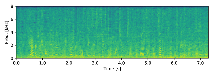
Figure 2: The observed spectrogram of noisy speech.

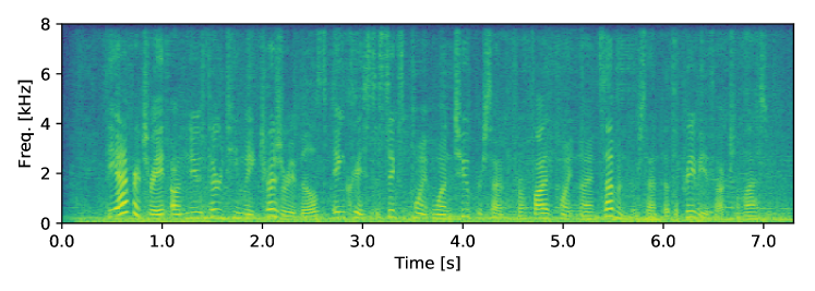
Figure 3: The enhanced spectrogram obtained by Beamformit.

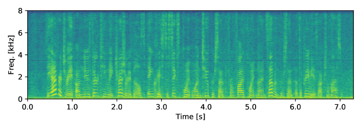
Figure 4: The enhanced spectrogram obtained by DNN-IBM.

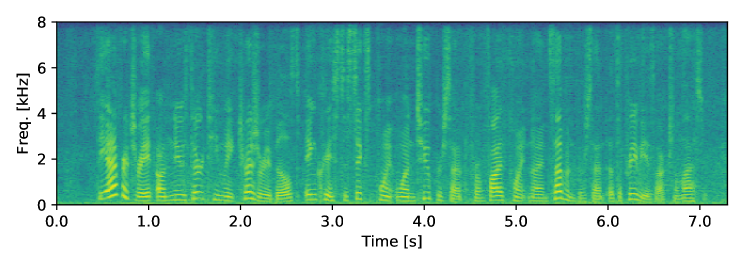
Figure 5: The enhanced spectrogram obtained by MNMF-TI-MV.

Interestingly, while the WERs obtained by the MNMF-based variants were much worse than those obtained by the DNN-based variants for the simulated data, all the methods yielded similar results for the real data. This indicates that the DNN-based beamforming tends to overfit the training data.

VI-B3 Speech Enhancement

The performances of speech enhancement are listed in Table IV. The MNMF-based variants were generally excellent in terms of the SDR, and were almost comparable with the DNN-based variants in terms of the PESQ and STOI. In our evaluation, the SDRs were closely related to the WERs. MNMF-TV-WF achieved the best average SDR of 16.16 dB, while the DNN-based variants showed lower SDRs up to 12.51 dB. Interestingly, the WERs obtained by the DNN-based variants were much better than those obtained by the MNMF-based variants for the simulated data. Figures 2, 3, 4, and 5 show the input noisy speech spectrogram and the enhanced speech spectrograms obtained by Beamformit, DNN-IBM, and MNMF-TI-MV, respectively. Although the low-frequency noise components were not sufficiently suppressed by the DNN-based methods, those components are considered to have a little impact on ASR. MNMF-TI-MV was shown to estimate harmonic structures more clearly.

The full-rank MWF worked best in speech enhancement and the rank-1 MWF showed the second highest performance. While the full-rank MWF can consider various propagation paths caused by reflection and reverberation, the rank-1 MWF and MVDR beamforming can consider only the direct paths from sound sources to the microphones. When the full-rank SCMs were accurately estimated by MNMF, the performance of speech enhancement was proven to be improved.

VI-C Evaluation on JNAS Dataset

We report the comparative experiment using the internal dataset recorded in real noisy environments. We also evaluated the online version of the proposed method.

VI-C1 Experimental Conditions

We made an internal dataset consisting of 200 sentences taken from the Japanese newspaper article sentence (JNAS) corpus [47] and spoken by five male speakers in a noisy crowded cafeteria (Fig. 6). The utterances were recorded with a five-channel microphone array ($M=5$) and the total duration was about 20 min. To make a realistic condition, we used a hemispherical array with micro-electro-mechanical system (MEMS) microphones that are widely used in commercial products. The distance between the speaker and the array was 1m. The noisy JNAS dataset has significantly different acoustic characteristics from those of the CHiME-3 dataset, as it was recorded in a different noisy environment by using a different microphone array (Table V).

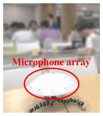
Figure 6: Recording environment for the noisy JNAS dataset.

TABLE V: Comparison of two ASR tasks.

Test set	CHiME-3	Noisy JNAS
Noisy environments	4 (including cafe)	1 (another cafe)
Microphone type	Condenser	MEMS
Microphone array geometry	Rectangle	Hemisphere
Speaker distance	0.2 - 0.5 m	1 m
Speaker gender	2 males & 2 females	5 male
Speaker language	English	Japanese

The ASR performance was evaluated using this dataset. The DNN-HMM acoustic model was also trained using the multi-condition data, in which the noise data of the CHiME-3 were added to the original clean 57,071 utterances of the JNAS. The model had six hidden layers with 2,048 sigmoidal nodes and an output layer with 3,000 nodes. A trigram language model was also trained using the JNAS. The Julius decoder [48] was used in this evaluation.

The noisy JNAS task was very different from the CHiME-3 task in terms of microphone setups and noise environments. Since the DNNs for mask estimation were trained using the noise data of the CHiME-3 data set, the noise condition of noisy JNAS was unknown. In noisy JNAS test sets, two kinds of DNNs were used for mask estimation. One was the same DNN as that in the CHiME-3 test sets. The other was trained by adding the noise data of the CHiME-3 to the original clean utterances of the JNAS corpus.

The online versions of the proposed MNMF-based variants were also evaluated. To investigate the length of the first mini-batch size, the online enhancement processing was performed using consecutive 10 utterances of the same speaker. For online speech enhancement, the basic mini-batch size was fixed to 0.5 s, and experiments were conducted by changing the size of the first mini-batch from 5 s to 20 s. They were compared with the offline processing with the consecutive 10 utterances. The value of the weight $\rho$ was set to 0.9.

VI-C2 Noisy Speech Recognition

TABLE VI: The experimental results of noisy speech recognition (WERs) with offline speech enhancement for the noisy JNAS data.

Method	Training data	Avg.
Not enhanced		38.52
Weighted DS		32.01
DNN-IBM	CHiME-3	12.27
DNN-IBM	JNAS	11.37
DNN-PSF	CHiME-3	12.11
DNN-PSF	JNAS	14.82
MNMF-TV-WF		10.01
MNMF-TI-WF		9.91
MNMF-TV-WF1		9.36
MNMF-TI-WF1		9.30
MNMF-TV-MV		9.30
MNMF-TI-MV		9.36

TABLE VII: The experimental results of noisy speech recognition (WERs) with online speech enhancement for the noisy JNAS data.

Method	Offline	Online
First mini-batch size		20 s	15 s	10 s	5 s
MNMF-TV-WF	9.10	9.07	9.07	9.55	11.32
MNMF-TI-WF	9.17	9.29	8.98	9.58	11.56
MNMF-TV-WF1	8.94	10.43	10.72	10.57	12.21
MNMF-TI-WF1	9.00	10.49	10.95	10.47	12.30
MNMF-TV-MV	8.71	9.95	11.94	11.21	12.84
MNMF-TI-MV	8.78	9.95	11.68	10.92	12.78

The performances of ASR are listed in Table VI. Training the DNN using the JNAS data used for training the DNN-HMM was effective (from 12.27% to 11.37%) because the speech data became matched in terms of spoken languages and noisy environments. MNMF-TI-WF1 and MNMF-TV-MV achieved the best WER of 9.30%, which was 18.21% relative improvement from that obtained by DNN-IBM trained by using the data used for training the DNN-HMM. The DNN-based beamforming was found to work worse in unknown recording conditions. This may have been due to over-fitting to the CHiME-3 noise data and it is difficult in practice to cover all the noisy conditions.

In the noisy JNAS tasks, there was also only a little difference among the beamforming methods, but the MVDR beamforming was the most effective in combination with the offline versions of the proposed method. The use of a time-variant noise SCM also did not bring notable improvement.

VI-C3 Online Speech Enhancement

The performances of ASR obtained by the online versions of the proposed method are listed in Table VII. The online MNMF-TI-WF achieved the average WER of 8.98% while the offline MNMF-TI-WF achieved the average WER of 9.17%. The performance of the online MNMF-TI-WF using a long first mini-batch was better than that of the offline version because the initial estimates of SCMs were accurate in all frequency bins. On the other hand, the performances of the online MNMF-TI-MV and MNMF-TI-WF1 were worse than those of the offline versions even when the first mini-batch was long. The offline MNMF-TI-MV achieved the average WER of 8.71% while the online MNMF-TV-MV achieved the average WER of 9.95%. MVDR beamforming and rank-1 MWF estimated the principal eigenvector of the SCM of speech as the steering vector for every mini-batch, which may degrade the ASR performance. The initialization of the online versions depends on the first mini-batch size. The performance was degraded when the first mini-batch contained a few segments of the target speech.

The practical problem of our approach lies in the computational complexity of MNMF related to the repeated inversions of SCMs. The real-time factors of the DNN- and MNMF-based beamforming methods were around 0.42 and 50, respectively. An order of magnitude faster approximations of MNMF [49, 50] was recently proposed, which was comparable with ILRMA in speed, and could be extended similarly to an online version for real-time noisy speech recognition.

The remaining problem lies in a long waiting time (10 s or 20 s) before achieving reasonable performance. This problem could be mitigated in a realistic scenario in which a microphone array (smart speaker) is assumed to be fixed in a room, e.g., a microphone array is placed on the center of a table for meeting recording. Every time sound activities are detected, the SCMs of the corresponding directions can be incrementally updated. A strong advantage of the proposed online method is that is can adapt to the room acoustics on the fly.

VI-D Experimental Findings

The two experiments using the CHiME-3 and JNAS datasets indicates that it is reasonable to use the MNMF-informed time-invariant rank-1 Wiener filtering (MNMF-TI-WF1) for dealing with noisy speech spectrograms recorded in real unseen environments. In online speech enhancement, the MNMF-informed time-invariant full-rank Wiener filtering (MNMF-TI-WF) tends to work best because the steering vector of speech is more difficult to update than the SCM of speech in an online manner. Since the WERs and SDRs obtained by the time-invariant beamforming methods are almost equal to those obtained by the time-variant methods, in practice it would be better to use the time-invariant methods for improving the temporal stability of speech enhancement.

VII Conclusion

This paper described the unsupervised speech enhancement method based MNMF-guided beamforming. Our method uses MNMF to estimate the SCMs of speech and noise in an unsupervised manner and then generates an enhanced speech signal with beamforming. We extended MNMF to an online version and initialized MNMF with ILRMA. We evaluated various types of beamforming in a wide variety of conditions. The experimental results in real-recording ASR tasks demonstrated that the proposed methods were more robust in an unknown environment than the state-of-the-art beamforming method with DNN-based mask estimation.

We plan to integrate BSS- and DNN-based SCM estimation in order to improve the performance of ASR. Learning a basis matrix from a clean speech database is expected to improve the performance of speech enhancement[37]. When a microphone array is specified beforehand, learning the normalized SCM of the target speech is also expected to improve the performance. When noisy environments are covered by training data used for DNN-based mask estimation, MNMF can be initialized by using the results of DNN-based mask estimation [2] to further refine the SCMs of speech and noise. It would be promising to use recently-proposed semi-supervised speech enhancement methods based on NMF or MNMF with a DNN-based prior on speech spectra [51, 52, 53].

Kazuki Shimada received the M.S. degree in informatics from Kyoto University, Kyoto, Japan, in 2018. He is currently working at Sony Corporation, Tokyo, Japan. His research interests include acoustic signal processing, automatic speech recognition, and statistical machine learning.

Yoshiaki Bando received the M.S. and Ph.D. degrees in informatics from Kyoto University, Kyoto, Japan, in 2015 and 2018, respectively. He is currently a Researcher at Artificial Intelligence Research Center (AIRC), National Institute of Advanced Industrial Science and Technology (AIST), Tokyo, Japan. His research interests include microphone array signal processing, deep Bayesian learning, and robot audition. He is a member of IEEE, RSJ, and IPSJ.

Masato Mimura received the B.E. and M.E. degrees from Kyoto University, Kyoto, Japan, in 1996 and 2000, respectively. He is currently a researcher in School of Informatics, Kyoto University.

Katsutoshi Itoyama received the M.S. and Ph.D. degrees in informatics from Kyoto University, Kyoto, Japan, in 2008 and 2011, respectively. He had been an Assistant Professor at the Graduate School of Informatics, Kyoto University, until 2018 and is currently a Senior Lecturer at Tokyo Institute of Technology. His research interests include sound source separation, music listening interfaces, and music information retrieval.

Kazuyoshi Yoshii received the M.S. and Ph.D. degrees in informatics from Kyoto University, Kyoto, Japan, in 2005 and 2008, respectively. He is an Associate Professor at the Graduate School of Informatics, Kyoto University, and concurrently the Leader of the Sound Scene Understanding Team, Center for Advanced Intelligence Project (AIP), RIKEN, Tokyo, Japan. His research interests include music informatics, audio signal processing, and statistical machine learning.

Tatsuya Kawahara received B.E. in 1987, M.E. in 1989, and Ph.D. in 1995, all in information science, from Kyoto University, Kyoto, Japan. From 1995 to 1996, he was a Visiting Researcher at Bell Laboratories, Murray Hill, NJ, USA. Currently, he is a Professor in the School of Informatics, Kyoto University. He has also been an Invited Researcher at ATR and NICT. He has published more than 300 technical papers on speech recognition, spoken language processing, and spoken dialogue systems. He has been conducting several projects including speech recognition software Julius and the automatic transcription system for the Japanese Parliament (Diet). Dr. Kawahara received the Commendation for Science and Technology by the Minister of Education, Culture, Sports, Science and Technology (MEXT) in 2012. From 2003 to 2006, he was a member of IEEE SPS Speech Technical Committee. He was a General Chair of IEEE Automatic Speech Recognition and Understanding workshop (ASRU 2007). He also served as a Tutorial Chair of INTERSPEECH 2010 and a Local Arrangement Chair of ICASSP 2012. He has been an editorial board member of Elsevier Journal of Computer Speech and Language and IEEE/ACM Transactions on Audio, Speech, and Language Processing. He is an editor in chief of APSIPA Transactions on Signal and Information Processing. Dr. Kawahara is a board member of APSIPA and ISCA, and a Fellow of IEEE.

References

- [1] T. Higuchi, N. Ito, S. Araki, T. Yoshioka, M. Delcroix, and T. Nakatani, “Online MVDR beamformer based on complex Gaussian mixture model with spatial prior for noise robust ASR,” IEEE/ACM Transactions on Audio, Speech, and Language Processing, vol. 25, no. 4, pp. 780–793, 2017.
- [2] T. Nakatani, N. Ito, T. Higuchi, S. Araki, and K. Kinoshita, “Integrating DNN-based and spatial clustering-based mask estimation for robust MVDR beamforming,” in IEEE International Conference on Acoustics, Speech and Signal Processing (ICASSP), 2017, pp. 286–290.
- [3] J. Heymann, L. Drude, and R. Haeb-Umbach, “Neural network based spectral mask estimation for acoustic beamforming,” in IEEE International Conference on Acoustics, Speech and Signal Processing (ICASSP), 2016, pp. 196–200.
- [4] H. Erdogan, J. R. Hershey, S. Watanabe, M. I. Mandel, and J. Le Roux, “Improved MVDR beamforming using single-channel mask prediction networks,” in Annual Conference of the International Speech Communication Association (Interspeech), 2016, pp. 1981–1985.
- [5] P. Pertilä, “Microphone-array-based speech enhancement using neural networks,” in Parametric Time-Frequency Domain Spatial Audio. Wiley-IEEE Press, 2017, pp. 291–325.
- [6] Z.-Q. Wang, J. L. Roux, and J. R. Hershey, “Multi-channel deep clustering: Discriminative spectral and spatial embeddings for speaker-independent speech separation,” in IEEE International Conference on Acoustics, Speech and Signal Processing (ICASSP), 2018, pp. 1–5.
- [7] X. Xiao, S. Zhao, D. L. Jones, E. S. Chng, and H. Li, “On time-frequency mask estimation for MVDR beamforming with application in robust speech recognition,” in IEEE International Conference on Acoustics, Speech and Signal Processing (ICASSP), 2017, pp. 3246–3250.
- [8] T. Ochiai, S. Watanabe, T. Hori, and J. R. Hershey, “Multichannel end-to-end speech recognition,” in International Conference on Machine Learning (ICML), vol. 70, 2017, pp. 2632–2641.
- [9] T. N. Sainath, R. J. Weiss, K. W. Wilson, B. Li, A. Narayanan, E. Variani, M. Bacchiani, I. Shafran, A. Senior, K. Chin, A. Misra, and C. Kim, “Multichannel signal processing with deep neural networks for automatic speech recognition,” IEEE/ACM Transactions on Audio, Speech, and Language Processing, vol. 25, no. 5, pp. 965–979, 2017.
- [10] M. Mimura, Y. Bando, K. Shimada, S. Sakai, K. Yoshii, and T. Kawahara, “Combined multi-channel NMF-based robust beamforming for noisy speech recognition,” in Annual Conference of the International Speech Communication Association (Interspeech), 2017, pp. 2451–2455.
- [11] M. Souden, J. Benesty, and S. Affes, “On optimal frequency-domain multichannel linear filtering for noise reduction,” IEEE Transactions on Audio, Speech, and Language Processing, vol. 18, no. 2, pp. 260–276, 2010.
- [12] Z. Wang, E. Vincent, R. Serizel, and Y. Yan, “Rank-1 constrained multichannel Wiener filter for speech recognition in noisy environments,” Computer Speech & Language, vol. 49, pp. 37–51, 2017.
- [13] B. D. Van Veen and K. M. Buckley, “Beamforming: A versatile approach to spatial filtering,” IEEE ASSP Magazine, vol. 5, no. 2, pp. 4–24, 1988.
- [14] S. Gannot and I. Cohen, “Speech enhancement based on the general transfer function GSC and postfiltering,” IEEE Transactions on Audio, Speech, and Language Processing, vol. 12, no. 6, pp. 561–571, 2004.
- [15] E. Warsitz and R. Haeb-Umbach, “Blind acoustic beamforming based on generalized eigenvalue decomposition,” IEEE Transactions on Audio, Speech, and Language Processing, vol. 15, no. 5, pp. 1529–1539, 2007.
- [16] J. Barker, R. Marxer, E. Vincent, and S. Watanabe, “The third CHiME speech separation and recognition challenge: Dataset, task and baselines,” in IEEE Automatic Speech Recognition and Understanding Workshop (ASRU), 2015, pp. 504–511.
- [17] T. Yoshioka, N. Ito, M. Delcroix, A. Ogawa, K. Kinoshita, M. Fujimoto, C. Yu, W. J. Fabian, M. Espi, T. Higuchi, S. Araki, and T. Nakatani, “The NTT CHiME-3 system: Advances in speech enhancement and recognition for mobile multi-microphone devices,” in IEEE Automatic Speech Recognition and Understanding Workshop (ASRU), 2015, pp. 436–443.
- [18] T. Hori, Z. Chen, H. Erdogan, J. R. Hershey, J. Le Roux, V. Mitra, and S. Watanabe, “The MERL/SRI system for the 3rd CHiME challenge using beamforming, robust feature extraction, and advanced speech recognition,” in IEEE Automatic Speech Recognition and Understanding Workshop (ASRU), 2015, pp. 475–481.
- [19] B. Loesch and B. Yang, “Adaptive segmentation and separation of determined convolutive mixtures under dynamic conditions,” in International conference on Latent Variable Analysis and Signal Separation (LVA/ICA), 2010, pp. 41–48.
- [20] X. Anguera, C. Wooters, and J. Hernando, “Acoustic beamforming for speaker diarization of meetings,” IEEE Transactions on Audio, Speech, and Language Processing, vol. 15, no. 7, pp. 2011–2022, 2007.
- [21] E. Vincent, S. Watanabe, A. A. Nugraha, J. Barker, and R. Marxer, “An analysis of environment, microphone and data simulation mismatches in robust speech recognition,” Computer Speech & Language, vol. 46, pp. 535–557, 2017.
- [22] K. Shimada, Y. Bando, M. Mimura, K. Itoyama, K. Yoshii, and T. Kawahara, “Unsupervised beamforming based on multichannel nonnegative matrix factorization for noisy speech recognition,” in IEEE International Conference on Acoustics, Speech and Signal Processing (ICASSP), 2018, pp. 5734–5738.
- [23] H. Sawada, H. Kameoka, S. Araki, and N. Ueda, “Multichannel extensions of non-negative matrix factorization with complex-valued data,” IEEE Transactions on Audio, Speech, and Language Processing, vol. 21, no. 5, pp. 971–982, 2013.
- [24] H. Erdogan, J. R. Hershey, S. Watanabe, and J. L. Roux, “Phase-sensitive and recognition-boosted speech separation using deep recurrent neural networks,” in IEEE International Conference on Acoustics, Speech and Signal Processing (ICASSP), 2015, pp. 708–712.
- [25] K. Itakura, Y. Bando, E. Nakamura, K. Itoyama, K. Yoshii, and T. Kawahara, “Bayesian multichannel audio source separation based on integrated source and spatial models,” IEEE/ACM Transactions on Audio, Speech, and Language Processing, vol. 26, no. 4, pp. 831–846, 2018.
- [26] A. Ozerov and C. Févotte, “Multichannel nonnegative matrix factorization in convolutive mixtures for audio source separation,” IEEE Transactions on Audio, Speech, and Language Processing, vol. 18, no. 3, pp. 550–563, 2010.
- [27] S. Arberet, A. Ozerov, and N. Q. K. Duong, “Nonnegative matrix factorization and spatial covariance model for under-determined reverberant audio source separation,” in IEEE International Conference on Information Science, Signal Processing and their Applications (ISSPA), 2010, pp. 1–4.
- [28] J. Nikunen and T. Virtanen, “Direction of arrival based spatial covariance model for blind sound source separation,” IEEE/ACM Transactions on Audio, Speech, and Language Processing, vol. 22, no. 3, pp. 727–739, 2014.
- [29] D. Kitamura, N. Ono, H. Sawada, H. Kameoka, and H. Saruwatari, “Determined blind source separation unifying independent vector analysis and nonnegative matrix factorization,” IEEE/ACM Transactions on Audio, Speech, and Language Processing, vol. 24, no. 9, pp. 1626–1641, 2016.
- [30] S. Doclo and M. Moonen, “GSVD-based optimal filtering for single and multimicrophone speech enhancement,” IEEE Transactions on Signal Processing, vol. 50, no. 9, pp. 2230–2244, 2002.
- [31] T. C. Lawin-Ore and S. Doclo, “Reference microphone selection for mwf-based noise reduction using distributed microphone arrays,” in ITG Symposium on Speech Communication, 2012, pp. 31–34.
- [32] Z. Wang, E. Vincent, R. Serizel, and Y. Yan, “Rank-1 constrained multichannel Wiener filter for speech recognition in noisy environments,” Computer Speech & Language, vol. 49, pp. 37–51, 2018.
- [33] T. Ando, C.-K. Li, and R. Mathias, “Geometric means,” Linear Algebra and its Applications, vol. 385, pp. 305–334, 2004.
- [34] W.-H. Chen, “A review of geometric mean of positive definite matrices,” British Journal of Mathematics & Computer Science, vol. 5, no. 1, pp. 1–12, 2015.
- [35] K. Yoshii, “Correlated tensor factorization for audio source separation,” in IEEE International Conference on Acoustics, Speech and Signal Processing (ICASSP), 2018, pp. 731–735.
- [36] A. Lefevre, F. Bach, and C. Févotte, “Online algorithms for nonnegative matrix factorization with the Itakura-Saito divergence,” in IEEE Workshop on Applications of Signal Processing to Audio and Acoustics (WASPAA), 2011, pp. 313–316.
- [37] Y. Tachioka, T. Narita, I. Miura, T. Uramoto, N. Monta, S. Uenohara, K. Furuya, S. Watanabe, and J. Le Roux, “Coupled initialization of multi-channel non-negative matrix factorization based on spatial and spectral information,” in Annual Conference of the International Speech Communication Association (Interspeech), 2017, pp. 2461–2465.
- [38] A. R. Mohamed, G. E. Dahl, and G. Hinton, “Acoustic modeling using deep belief networks,” IEEE Transactions on Audio, Speech, and Language Processing, vol. 20, no. 1, pp. 14–22, 2012.
- [39] G. E. Dahl, D. Yu, L. Deng, and A. Acero, “Context-dependent pre-trained deep neural networks for large-vocabulary speech recognition,” IEEE Transactions on Audio, Speech, and Language Processing, vol. 20, no. 1, pp. 30–42, 2012.
- [40] D. Povey, A. Ghoshal, G. Boulianne, L. Burget, O. Glembek, N. Goel, M. Hannemann, P. Motlíček, Y. Qian, P. Schwarz, J. Silovský, G. Stemmer, and K. Veselý, “The Kaldi speech recognition toolkit,” in IEEE Automatic Speech Recognition and Understanding Workshop (ASRU), 2011.
- [41] V. Nair and G. E. Hinton, “Rectified linear units improve restricted Boltzmann machines,” in International Conference on Machine Learning (ICML), 2010, pp. 807–814.
- [42] N. Srivastava, G. Hinton, A. Krizhevsky, I. Sutskever, and R. Salakhutdinov, “Dropout: A simple way to prevent neural networks from overfitting.” Journal of Machine Learning Research, vol. 15, no. 1, pp. 1929–1958, 2014.
- [43] S. Ioffe and C. Szegedy, “Batch normalization: Accelerating deep network training by reducing internal covariate shift,” in International Conference on Machine Learning (ICML), 2015, pp. 448–456.
- [44] E. Vincent, R. Gribonval, and C. Févotte, “Performance measurement in blind audio source separation,” IEEE Transactions on Audio, Speech, and Language Processing, vol. 14, no. 4, pp. 1462–1469, 2006.
- [45] A. Rix, J. Beerends, M. Hollier, and A. Hekstra, “Perceptual evaluation of speech quality (PESQ), an objective method for end-to-end speech quality assessment of narrowband telephone networks and speech codecs,” in ITU-T Recommendation. IEEE, 2001, p. 862.
- [46] C. H. Taal, R. C. Hendriks, R. Heusdens, and J. Jensen, “An algorithm for intelligibility prediction of time-frequency weighted noisy speech,” IEEE Transactions on Audio, Speech, and Language Processing, vol. 19, no. 7, pp. 2125–2136, 2011.
- [47] K. Itou, M. Yamamoto, K. Takeda, T. Takezawa, T. Matsuoka, T. Kobayashi, K. Shikano, and S. Itahashi, “JNAS: Japanese speech corpus for large vocabulary continuous speech recognition research,” Journal of the Acoustical Society of Japan (E), vol. 20, no. 3, pp. 199–206, 1999.
- [48] A. Lee, T. Kawahara, and K. Shikano, “Julius — An open source real-time large vocabulary recognition engine,” in European Conference on Speech Communication and Technology (Eurospeech), 2001, pp. 1691–1694.
- [49] N. Ito and T. Nakatani, “FastMNMF: Joint diagonalization based accelerated algorithms for multichannel matrix factorization,” in IEEE International Conference on Acoustics, Speech and Signal Processing (ICASSP), 2019, to appear.
- [50] K. Sekiguchi, A. A. Nugraha, Y. Bando, and K. Yoshii, “Fast multichannel source separation based on jointly diagonalizable spatial covariance matrices,” in European Signal Processing Conference (EUSIPCO), 2019, submitted. [Online]. Available: https://arxiv.org/abs/1903.03237
- [51] Y. Bando, M. Mimura, K. Itoyama, K. Yoshii, and T. Kawahara, “Statistical speech enhancement based on probabilistic integration of variational autoencoder and non-negative matrix factorization,” in IEEE International Conference on Acoustics, Speech and Signal Processing (ICASSP), 2018, pp. 716–720.
- [52] S. Leglaive, L. Girin, and R. Horaud, “A variance modeling framework based on variational autoencoders for speech enhancement,” in IEEE International Workshop on Machine Learning for Signal Processing (MLSP), 2018, pp. 1–6.
- [53] K. Sekiguchi, Y. Bando, K. Yoshii, and T. Kawahara, “Bayesian multichannel speech enhancement with a deep speech prior,” in Asia-Pacific Signal and Information Processing Association Annual Summit and Conference (APSIPA ASC), 2018, pp. 1233–1239.