Optimization Methods for Interpretable Differentiable Decision Trees in Reinforcement Learning
Andrew Silva Taylor Killian Ivan Rodriguez Jimenez Georgia Institute of Technology University of Toronto Georgia Institute of Technology
Sung-Hyun Son Matthew Gombolay MIT Lincoln Laboratory Georgia Institute of Technology
Abstract
Decision trees are ubiquitous in machine learning for their ease of use and interpretability. Yet, these models are not typically employed in reinforcement learning as they cannot be updated online via stochastic gradient descent. We overcome this limitation by allowing for a gradient update over the entire tree that improves sample complexity affords interpretable policy extraction. First, we include theoretical motivation on the need for policy-gradient learning by examining the properties of gradient descent over differentiable decision trees. Second, we demonstrate that our approach equals or outperforms a neural network on all domains and can learn discrete decision trees online with average rewards up to 7x higher than a batch-trained decision tree. Third, we conduct a user study to quantify the interpretability of a decision tree, rule list, and a neural network with statistically significant results ().
1 Introduction and Related Work
Reinforcement learning (RL) with neural network function approximators, known as “Deep RL,” has achieved tremendous results in recent years (Andrychowicz et al., 2018, 2016; Arulkumaran et al., 2017; Espeholt et al., 2018; Mnih et al., 2013; Sun et al., 2018; Rajeswaran et al., 2017). Deep RL uses multi-layered neural networks to represent policies trained to maximize an agent’s expected future reward. Unfortunately, these neural-network-based approaches are largely uninterpretable due to the millions of parameters involved and nonlinear activations throughout.
In safety-critical domains, e.g., healthcare and aviation, insight into a machine’s decision-making process is of utmost importance. Human operators must be able to follow step-by-step procedures (Gawande, 2010; Haynes, 2009) or hold machines accountable (Natarajan and Gombolay, 2020). Of the machine learning (ML) methods able to generate such procedures, decision trees are among the most highly developed (Weiss and Indurkhya, 1995), persisting in use today (Gombolay et al., 2018a; Zhang et al., 2019). While interpretable ML methods offer much promise (Letham et al., 2015), they are unable to match the performance of Deep RL (Finney, 2002; Silver, 2016). In this paper, we advance the state of the art in decision tree methods for RL and leverage their ability to yield interpretable policies.
Decision trees are viewed as the de facto technique for interpretable and transparent ML (Rudin, 2014; Lipton, 2018), as they learn compact representations of relationships within data (Breiman et al., 1984). Rule (Angelino et al., 2017; Chen and Rudin, 2017) and decision lists (Lakkaraju and Rudin, 2017; Letham et al., 2015) are related architectures also used to communicate a decision-making process. Decision trees have been also applied to RL problems where they served as function approximators, representing which action to take in which state (Ernst and Wehenkel, 2005; Finney, 2002; Pyeatt and Howe, 2001; Shah and Gopal, 2010).
The challenge for decision trees as function approximators lies in the online nature of the RL problem. The model must adapt to the non-stationary distribution of the data as the model interacts with its environment. The two primary techniques for learning through function approximation, Q-learning (Watkins, 1989) and policy gradient (Sutton and Mansour, 2000), rely on online training and stochastic gradient descent (Bottou, 2010; Fletcher and Powell, 1963). Standard decision trees are not amenable to gradient descent as they are a collection of non-differentiable, nested, if-then rules. As such, researchers have used non-gradient-descent-based methods for training decision trees for RL (Ernst and Wehenkel, 2005; Finney, 2002; Pyeatt and Howe, 2001), e.g., greedy state aggregation, rather than seeking to update the entire model with respect to a global loss function (Pyeatt and Howe, 2001). Researchers have also attempted to use decision trees for RL by training in batch mode, completely re-learning the tree from scratch to account for the non-stationarity introduced by an improving policy (Ernst and Wehenkel, 2005). This approach is inefficient when scaling to realistic situations and is not guaranteed to converge. Despite these attempts, success comparable to that of modern deep learning approaches has been elusive (Finney, 2002).
In this paper, we present an novel function approximation technique for RL via differentiable decision trees (DDTs). We provide three contributions. First, we examine the properties of gradient descent over DDTs, motivating policy-gradient-based learning. To our knowledge, this is the first investigation of the optimization surfaces of Q-learning and policy gradients for DDTs. Second, we compare our method with baseline approaches on standard RL challenges, showing that our approach parities or outperforms a neural network; further, the interpretable decision trees we discretize after training achieve an average reward up to 7x higher than a batch-learned decision tree. Finally, we conduct a user study to compare the interpretability and usability of each method as a decision-making aid for humans, showing that discrete trees and decision lists are perceived as more helpful () and are objectively more efficient () than a neural network.
Remark 1 (Analysis Significance)
Our approach builds upon decades of work in machine and RL; yet ours is the first to consider DDTs for online learning. While researchers have shown failings of Q-learning with function approximation, including for sigmoids (Baird, 1995; Bertsekas and Tsitsiklis, 1996; Gordon, 1995; Tsitsiklis and Van Roy, 1996), we are unaware of analysis of Q-learning and policy gradient for our unique architecture. Our analysis provides insight regarding the best practices for training interpretable RL policies with DDTs.
2 Preliminaries
In this section, we review decision trees, DDTs, and RL.
2.1 Decision Trees
A decision tree is a directed, acyclic graph, with nodes and edges, that takes as input an example, , performs a forward recursion, and returns a label ( Eq. 1-3).
| (1) | ||||
| (2) | ||||
| (3) |
There are two node types: decision and leaf nodes, which have an outdegree of two and zero, respectively. Nodes have an indegree of one except for the root, , whose indegree is zero. Decision nodes are represented as Boolean expressions, (Eq. 3), where and are the selected feature and splitting threshold for decision node . For each decision node, the left outgoing edge is labeled “true,” and the right outgoing edge is labeled “false.” E.g., if is evaluated true, the left child node, , is considered next. The process repeats until a leaf is reached upon which the tree returns the corresponding label. The goal is to determine the best , , and for each node and the best structure (i.e., whether, for each , there exists a child). There are many heuristic techniques for learning decision trees with a batch data (Breiman et al., 1984). However, one cannot apply gradient updates as the tree is fixed at generation. While some have sought to grow trees for RL (Pyeatt and Howe, 2001), these approaches do not update the entire tree.
DDTs –
Suárez and Lutsko provide one of the first DDT models. Their method replaces the Boolean decision in Eq. 3 with the sigmoid activation function shown in Eq. 4. This function considers a linear combination of features weighted by compared to a bias value , and augmented by a steepness parameter . The tree is trained via gradient descent for, , , and across nodes (Suárez and Lutsko, 1999). This method has been applied to offline, supervised learning but not RL.
| (4) |
2.2 Reinforcement Learning
RL is a subset of machine learning in which an agent is tasked with learning the optimal action sequence that maximizes future expected reward (Sutton and Barto, 1998). The problem is abstracted as a Markov Decision Process (MDP), which is a five-tuple defined as follows: is the set of states; is the set of actions; is the transition matrix describing the probability that taking action in state results in state ; is the discount factor defining the trade-off between immediate and future reward; and is the function dictating the reward an agent receives by taking action in state . The goal is to learn a policy, , that prescribes which action to take in each state to maximize the agent’s long-term expected reward. There are two ubiquitous approaches to learn a policy: Q-learning and policy gradient.
Q-learning seeks to to learn a mapping, , that returns the expected future reward when taking action in state . This mapping (i.e., the Q-function) is typically approximated by a parameterization (e.g., a neural network), . One then minimizes the Bellman residual via Eq. 5, where is the estimated change in , and is the state the agent arrives in after applying action in state at time step with learning rate .
| (5) |
A complementary approach is the set of policy gradient methods in which one seeks to directly learn a policy, , parameterized by , that maps states to actions. The update rule maximizes the expected reward of a policy, as shown in Eq. 6, where indicates the change in for a timestep under policy gradient and . is the length of the trajectory.
| (6) |
We provide an investigation into the behavior of and as for DDTs in Section 5.
3 DDTs as Interpretable Function Approximators
In this section, we derive the Q-learning and policy gradient updates for DDTs as function approximators in RL. Due to space considerations, we show the simple case of a DDT with a single decision node and two leaves with one feature with feature coefficient , as shown in Eq. 7 with the gradient shown in Equations 8-12.
| (7) | |||
| (8) | |||
| (9) | |||
| (10) | |||
| (11) |
| (12) |
When utilizing a DDT as a function approximator for Q-learning, each leaf node returns an estimate of the expected future reward (i.e., the Q-value) for applying each action when in the portion of the state space dictated by the criterion of it’s parent node (Eq. 13).
| (13) |
Likewise, when leveraging policy gradient methods for RL with DDT function approximation, the leaves represent an estimate of the optimal probability distribution over actions the RL agent should take to maximize its future expected reward. Therefore, the values at these leaves represent the probability of selecting the corresponding action (Eq. 14). We impose the constraint that the probabilities of all actions sum to one ().
| (14) |
4 Interpretability for Online Learning
We seek to address the two key drawbacks of the original DDT formulation by Suárez and Lutsko (Suárez and Lutsko, 1999) in making the tree interpretable. First, the operation at each node produces a linear combination of the features, rather than a single feature comparison. Second, use of the sigmoid activation fuction means that there is a smooth transition between the and evaluations of a node, rather than a discrete decision. We address these limitations below; we demonstrate the extensibility of our approach by also differentiating over a rule list architecture (Letham et al., 2015) and extracting interpretable rule lists. Using the mechanisms from Sections 4.1 and 4.2, we produce interpretable policies for empirical evaluation (Section 6) and a user study (Section 7).
4.1 Discretizing the Differentiable Decision Tree
Due to the nature of the sigmoid function, even a sparse is not sufficient to guarantee a discrete decision at each node. Thus, to obtain a truly discrete tree, we convert the differentiable tree into a discrete tree by employing an to obtain the index of the feature of that the node will use. We set to a one-hot vector, with a at index and elsewhere. We also divide by the node’s weight , normalizing the value for comparison against the raw input feature . Each node then compares a single raw input feature to a single , effectively converting from Eq. 4 back into Eq. 3. We repeat this process for each decision node, obtaining discrete splits throughout the tree. Finally, each leaf node must now return a single action, as in an ordinary decision tree. We again employ an on each leaf node and set the leaves to be one-hot vectors with and all other values set to . The result of this process is an interpretable decision tree with discrete decision nodes, a single feature comparison per node, and a single decision output per leaf.
4.2 Differentiable Rule Lists
In addition to discretizing the optimized tree parameterization, we also consider a specific sub-formulation of tree proposed by (Letham et al., 2015) to be particularly interpretable: the rule- or decision-list. This type of tree restricts the symmetric branching allowed for in Eq. 1 by stating that the TRUE branch from a decision node leads directly to a leaf node. We define a discrete rule list according to Eq. 15.
| (15) |
In Section 6, we demonstrate that these mechanisms for interpretability achieves high-quality policies for online RL and are consistent with the the legal (Voigt and Von dem Bussche, 2017) and practical criteria for interpretability (Doshi-Velez and Kim, 2017; Letham et al., 2015).
5 Analysis of Gradient Methods for DDTs
In this section, we analyze Q-learning and policy gradient updates for DDTs as function approximators in RL, providing a theoretical basis for how to best deploy DDTs to RL. We show that Q-learning introduces additional critical points that impede learning where policy gradient does not. This analysis guides us to recommend policy gradient for these interpretable function approximators and yields high-quality policies (Section 6).
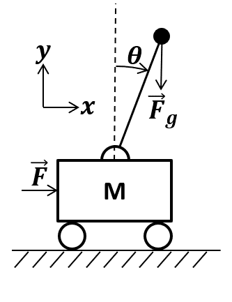
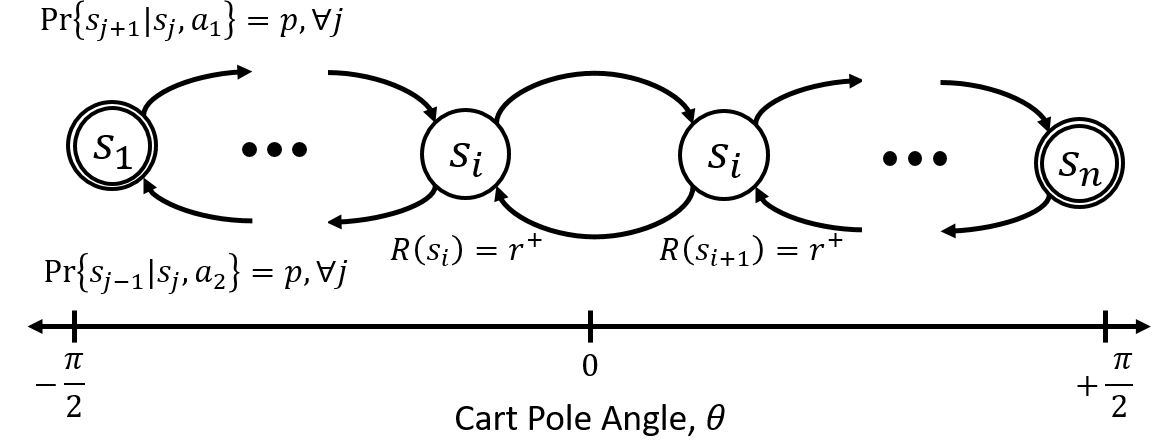
5.1 Analysis: Problem Setup
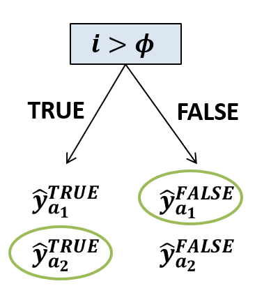
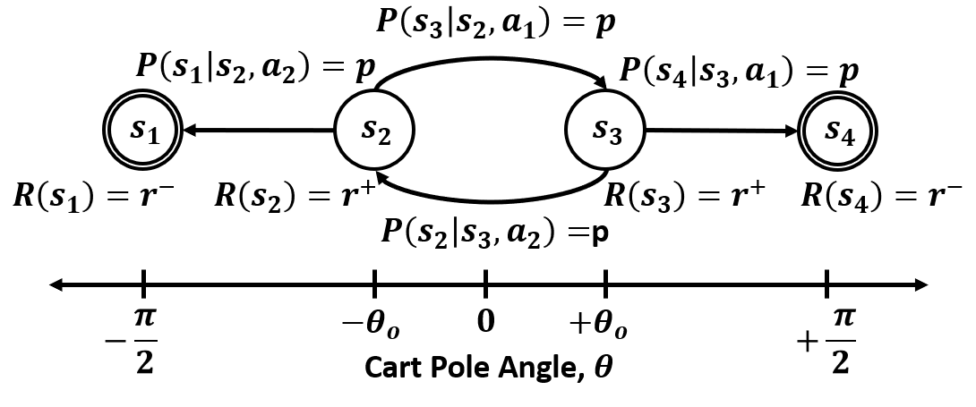
We consider an MDP with states and actions (Figure 1(b)). The agent moves to a state with a higher index (i.e., ) when taking action with probability and for transitioning to a lower index. The opposite is the case for action . Within Figure 1(b), corresponds to “move right” and corresponds to “move left.” The terminal states are and . The rewards are zero for each state except for for some such that . It follows that the optimal policy, , is (“move right”) in such that and otherwise. A proof is given in supplementary material. We optimistically assume ; despite this hopeful assumption, we show unfavorable results for Q-learning and policy-gradient-based agents using DDTs as function approximators.
5.2 Analysis: Tree Initialization
For our investigation, we assume that the decision tree’s parameters are initialized to the optimal setting. Given our MDP setup, we only have one state feature: the state’s index. As such, we only have two degrees of freedom in the decision node: the steepness parameter, , and the splitting criterion, . In our analysis, we focus on this splitting criterion, , showing that even for an optimal tree initialization, is not compelled to converge to the optimal setting . We set the leaf nodes as follows for Q-learning and policy gradient given the optimal policy.
For Q-learning, we set the discounted optimal action reward as , which assumes . Likewise, we set , which correspond to the Q-values of taking action and in states and when otherwise following the optimal policy starting in a non-terminal node.
For policy gradient, we set and . These settings correspond to a decision tree that focuses on exploiting the current (optimal if ) policy. While we consider this setting of parameters for our analysis of DDTs, the results generalize.
5.3 Computing Critical Points
The ultimate step in our analysis is to assess whether Q-learning or policy gradient introduces critical points that do not coincide with global extrema. To do so, we can set Equations 5 and 6 to zero, with from Eq. 13 and from Eq. 14, respectively. We would then solve for our parameter(s) of interest and determine whether any zeros lie at local extrema. In our case, focusing on the splitting criterion, , is sufficient to show the weaknesses of Q-learning for DDTs.
Rather than exactly solving for the zeros, we use numerical approximation for these Monte Carlo updates (Equations 5 and 6). In this setting, we recall that the agent experiences episodes with timesteps. Each step generates its own update, which are combined to give the overall update . Pseudo-critical points exist, then, whenever = 0. A gradient descent algorithm would treat these as extrema, and the gradient update would push towards these points. As such, we consider these “critical points.”
5.4 Numerical Analysis of the Updates
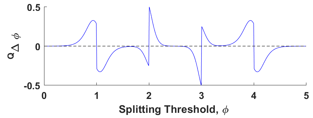
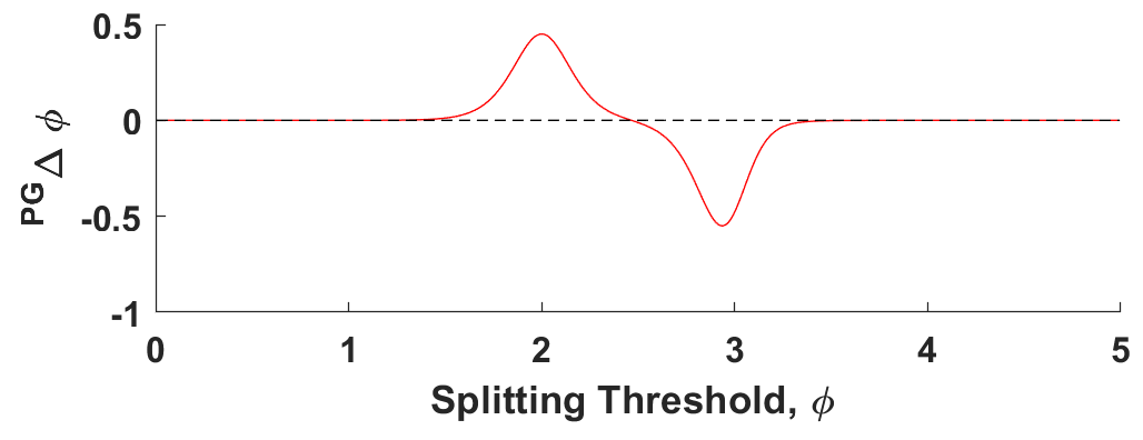
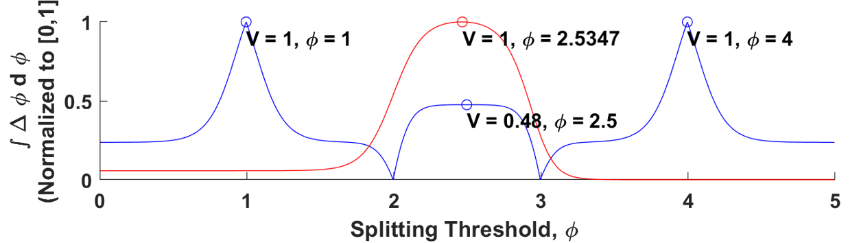
The critical points given by are shown in Fig. 2(a) and 2(c) for Q-learning and PG, respectively. For the purpose of illustration, we set (i.e., the MDP has four states). As such, and the optimal setting for .
For Q-learning, there are five critical points, only one of which is coincident with . For PG, there are fewer, with a single critical point in the domain of , which occurs at 111We recall that, for this analysis, ; if we set (i.e., the symmetric position with respect to vertical), this critical point for policy gradient is .. Thus, we can say that the expectation of the critical point for a random, symmetric initialization is , which supports the adoption of policy gradient as an approach for DDTs.
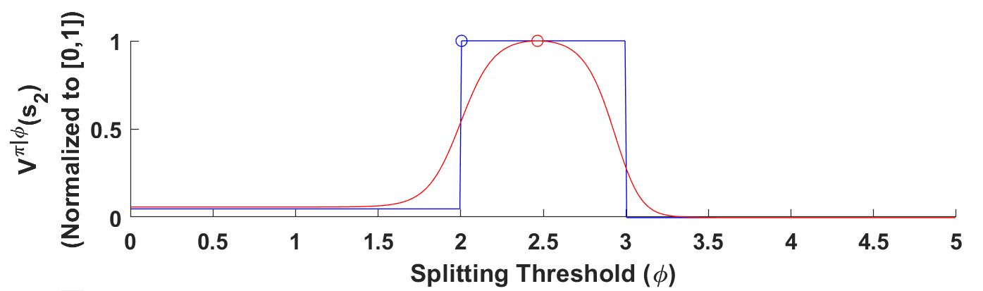
Additionally, by integrating with respect to from to , i.e., , we infer the “optimality curve,” which should equal the value of the policy, , implied by Q-learning and policy gradient. We numerically integrate using Riemann’s method normalized to . One would expect that the respective curves for the policy value (Figure 2(b)) and integrated gradient updates (Figure 2(d)) would be identical; however, this does not hold for Q-learning. Q-learning with DDT function approximation introduces undesired extrema, shown by the blue curve in Figure 2(d). Policy gradient, on the other hand, maintains a single maximum coincident with .
This analysis provides evidence that Q-learning exhibits weaknesses when applied to DDT models, such as an excess of critical points which serve to impede gradient descent. We therefore conclude that policy gradient is a more promising approach for learning the parameters of DDTs and proceed accordingly. As such, we have shown that Q-learning with DDT function approximators introduces additional extrema that policy gradients, under the same conditions, do not, within our MDP case study.
This analysis provides the first examination of the potential pitfalls and failings of Q-learning with DDTs. We believe that this helpful analysis will guide researchers in the application of these function approximators. Given this analysis and our mechanisms for interpretability (Section 4), we now show convincing empirical results (Section 6) of the power of these function approximators to achieve high-quality and interpretable policies in RL.
6 Demonstration of DDTs for Online RL
Our ultimate goal is to show that DDTs can learn competent, interpretable policies online for RL tasks. To demonstrate this, we evaluate our DDT algorithm using the cart pole and lunar lander OpenAI Gym environments (Brockman et al., 2016), a simulated wildfire tracking problem, and the FindAndDefeatZerglings mini-game from the StarCraft II Learning Environment (Vinyals et al., 2017). All agents are trained via Proximal Policy Optimization (PPO) (Kostrikov, 2018; Schulman et al., 2017). We use a multilayer perceptron (MLP) architecture as a baseline for performance across all tasks. We provide further details on the evaluation domains below, as well as examples of extracted interpretable policies, trained using online RL with DDTs. Due to space constraints, we present pruned versions of the interpretable policies in which redundant nodes are removed for visual clarity. The full policies are in the supplementary material.
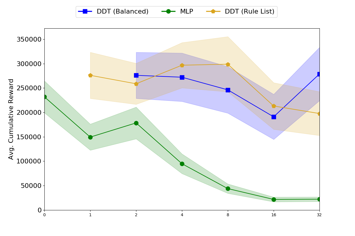
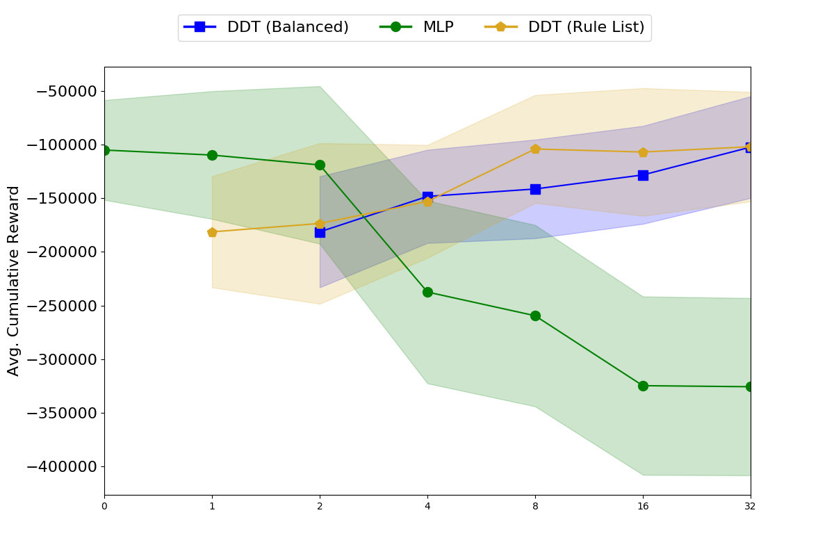
We conduct a sensitivity analysis comparing the performance of MLPs with DDTs (DDTs) across a range of depths. For the trees, the set of leaf nodes we consider is {2, 4, 8, 16, 32}. For comparison, we run MLP agents with between {0, 1, 2, 4, 8, 16, 32} hidden layers, and a rule-list architecture with {1, 2, 4, 8, 16, 32} rules. Results from this sensitivity analysis are given in Fig. 4 & 5 in the supplementary material. We find that MLPs succeed only with a narrow subset of architectures, while DDTs and rule lists are more robust. In this section, we present results from the agents that obtained the highest average cumulative reward in our sensitivity analysis. Table 1 compares mean reward of the highest-achieving agents and shows the mean reward for our discretization approach applied to the best agents. For completeness, we also compare against standard decision trees which are fit using scikit-learn (Pedregosa, 2011) on a set of state-action pairs generated by the best-performing model in each domain, which we call State-Action DT.
In our OpenAI Gym (Brockman et al., 2016) environments we use a learning rate of 1e-2, and in our wildfire tracking and FindAndDefeatZerglings (Vinyals et al., 2017) domains we use a learning rate of 1e-3. All models are updated with the RMSProp (Tieleman and Hinton, 2012) optimizer. All hyperparameters are included in the supplementary material.
| Agent Type | Cart Pole | Lunar Lander | Wildfire Tracking | FindAndDefeatZerglings |
|---|---|---|---|---|
| DDT Balanced Tree (ours) | 500 0 | 97.9 10.5 | -32.0 3.8 | 6.6 1.1 |
| DDT Rule List (ours) | 500 0 | 84.5 13.6 | -32.3 4.8 | 11.3 1.4 |
| MLP | 500 0 | 87.7 21.3 | -86.7 9.0 | 6.6 1.2 |
| Discretized DDT (ours) | 499.5 0.8 | -88 20.4 | -36.4 2.6 | 4.2 1.6 |
| Discretized Rule List (ours) | 414.4 63.9 | -78.4 32.2 | -39.8 1.8 | 0.7 1.3 |
| State-Action DT | 66.3 18.5 | -280.9 60.6 | -67.9 7.9 | -3.0 0.0 |
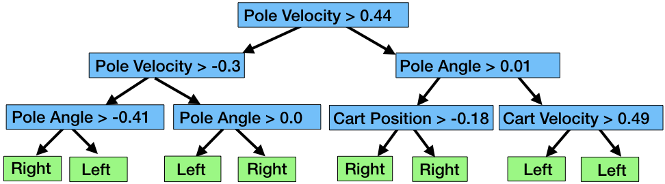
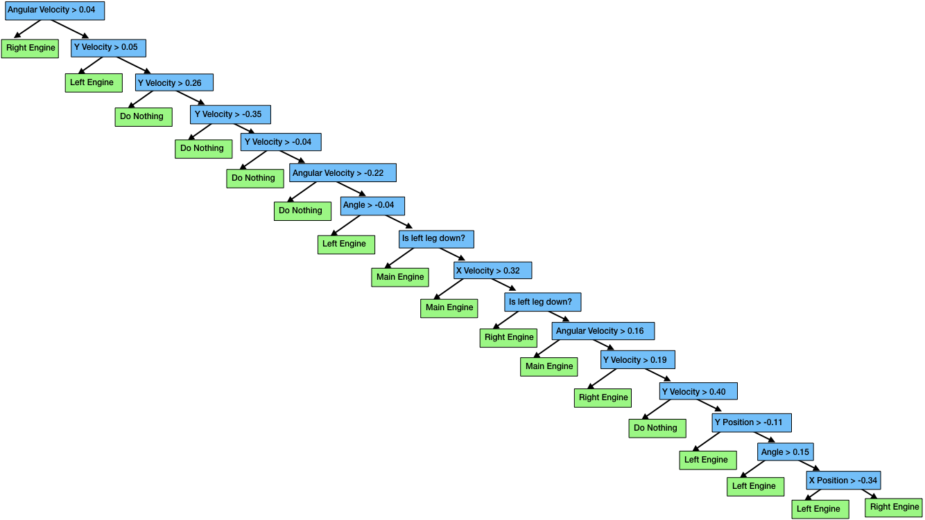
6.1 Open AI Gym Evaluation
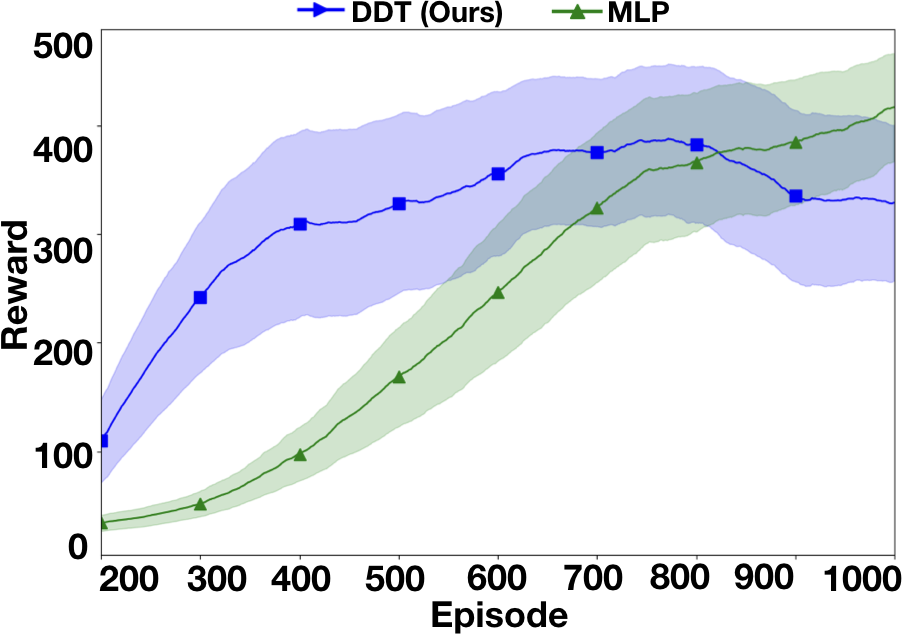
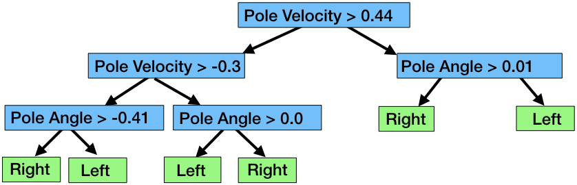
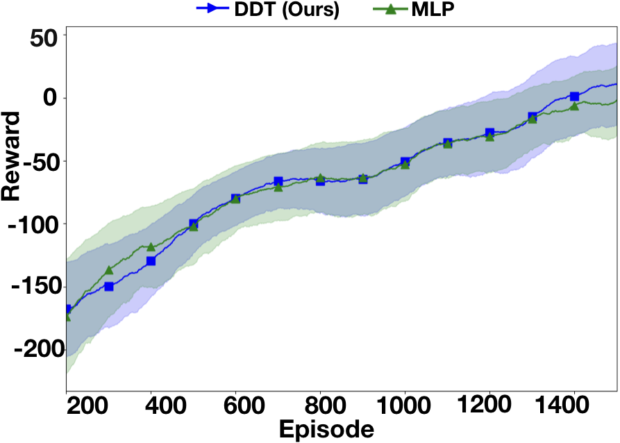
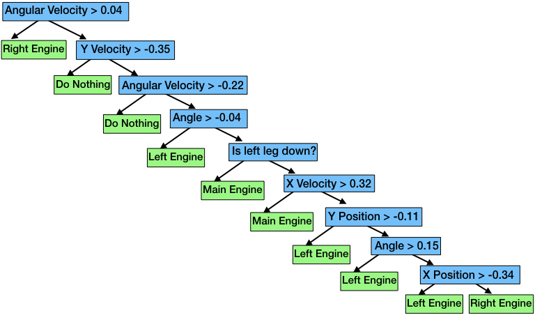
We plot the performance of the best agent for each architecture in our OpenAI Gym (Brockman et al., 2016) experiments, as well as pruned interpretable policies, in Fig. 3 and 4. To show the variance of the policies, we run five seeds for each policy-environment combination. Given the flexibility of MLPs and their large number of parameters, we anticipate an advantage in raw performance. We find that the DDT offers competitive or even superior performance compared to the MLP baseline, and even after converting the trained DDT into a discretized, interpretable tree, the training process yields tree policies that are competitive with the best MLP. Our interpretable approach yields a 3x and 7x improvement over a batch-trained decision tree (DT) on lunar lander and cart pole, respectively. Table 1 depicts the average reward across domains and agents.
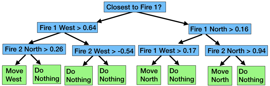
6.2 Wildfire Tracking
Wildfire tracking is a real-world problem in which interpretability is critical to an agent’s human teammates. While RL is a promising approach to develop assistive agents in wildfire monitoring (Haksar and Schwager, 2018), it is important to maintain trust between these agents and humans in this dangerous domain. An agent that can explicitly give its policy to a human firefighter is therefore highly desirable.
We develop a Python implementation of the simplified FARSITE (Finney, 1998) wildfire propagation model. The environment is a 500x500 map in which two fires propagate slowly from the southeast end of the map to the northwest end of the map and two drones are randomly instantiated in the map. Each drone receives a 6D state containing distances to each fire centroid and Boolean flags indicating which fire the drone is closer to. The RL agent is duplicated at the start of each episode and applied to each drone, and the drones do not have any way of communicating. The challenge is to identify which fire is closest to the drone, and to then take action to get as close as possible to that fire centroid, with the objective of flying above the fires as they progress across the map. Available actions include four move commands (north, east, south, west) and a “do nothing” command. The reward function is the negative distance from drones to fires, given in Eq. 16 where is a distance function, are the drones, and are the fires.
| (16) |
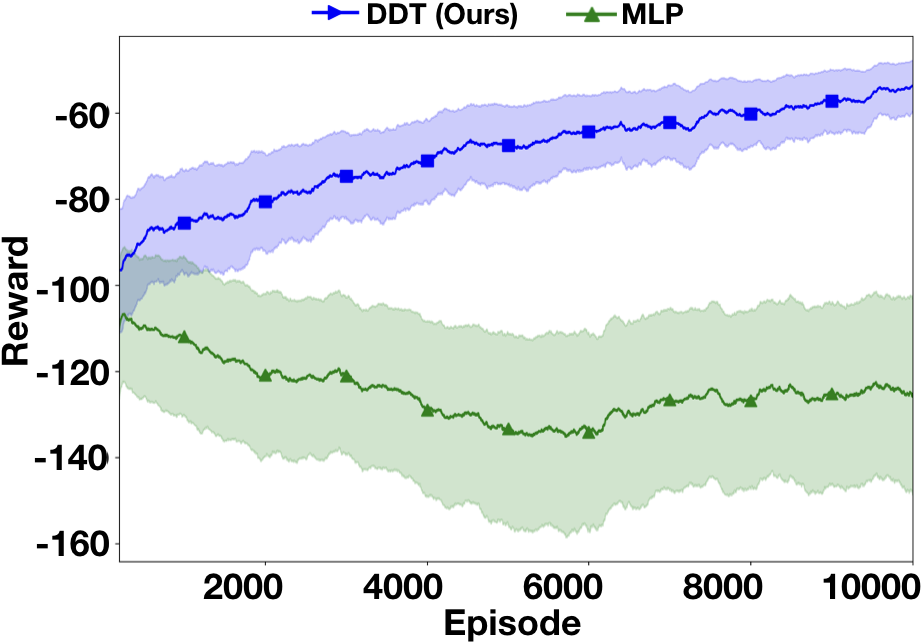
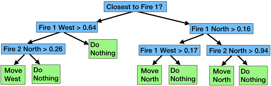
The reward over time for the top performing DDT and MLP agents is given in Figure 5, showing the DDT significantly outperforms the MLP. We also present the interpretable policy for the best DDT agent, which has the agent neglect the south and east actions, instead checking for north and west distances and moving in those directions. This behavior reflects the dynamics of the domain, in which the fire always spreads from southeast to northwest. The best interpretable policy we learn is 2x better than the best batch-learned tree and 2x better than the best MLP.
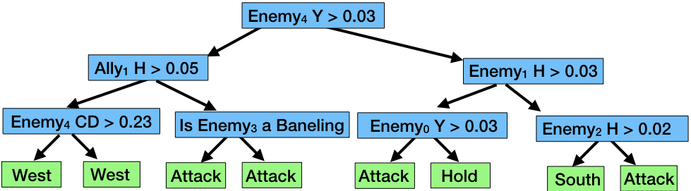
6.3 StarCraft II Micro-battle Evaluation
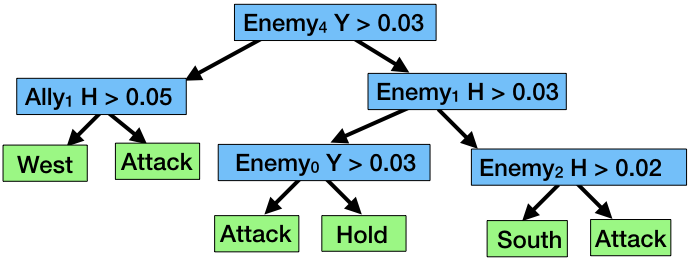
To further evaluate the DDT and discretized tree, we use the FindAndDefeatZerglings minigame from the StarCraft II Learning Environment (Vinyals et al., 2017). For this challenge, three allied units explore a partially observable map and defeat as many enemy units as possible within three minutes. We assign each allied unit a copy of the same learning agent. Rather than considering the image input and keyboard and mouse output, we manufacture a reduced state-action space. The input state is a 37D vector of allied and visible enemy state information, and the action space is 10D consisting of move and attack commands. More information is in supplementary material.
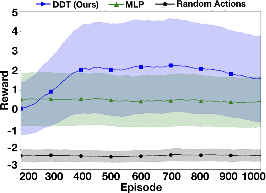
As we can see in Figure 6, our DDT agent is again competitive with the MLP agent and is 2x better than a batch-learned decision tree. The interpretable policy for the best DDT agent reveals that the agent frequently chooses to attack, and never moves in conflicting directions. This behavior is intuitive, as the three allied units should stay grouped to increase their chances of survival. The agent has learned not to send units in conflicting directions, instead moving units southwest while attacking enemies en route.
7 Interpretability Study
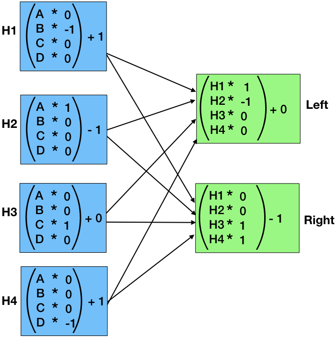
To emphasize the interpretability afforded by our approach, we conducted a user study in which participants were presented with policies trained in the cart pole domain and tasked with identifying which decisions the policies would have made given a set of state inputs. We compared interpretability between a discrete decision tree, a decision list, and a one-hot MLP without activation functions.
7.1 Study Setup
We designed an online questionnaire to survey 15 participants, giving each a discretized DDT, a discretized decision list, and a sample one-hot MLP. The discretized policies are actual policies from our experiments, presented in Table 1. Rather than include the full MLP, which is available in the supplementary material, we binarized the weights, thereby make the calculation much easier and less frustrating for participants. This mechanism is similar to current approaches to interpretability with deep networks that use attention (Serrano and Smith, 2019) so that human operators can see what the agent is considering when it makes a decision.
After being given a policy, participants were presented with five sample domain states. They were then asked to trace the policy with a given input state and predict what the agent would have done. After predicting which decisions the agent would have made, participants were presented with a set of Likert scales assessing their feelings on the interpretability and usability of the given policy as a decision-making aid. We timed participants for each method.
We hypothesize that: H1: A decision-based classifier is more interpretable than an MLP; H2: A decision-based classifier is more efficient than a MLP. To test these hypotheses, we report on participant Likert scale ratings (H1) and completion time for each task (H2).
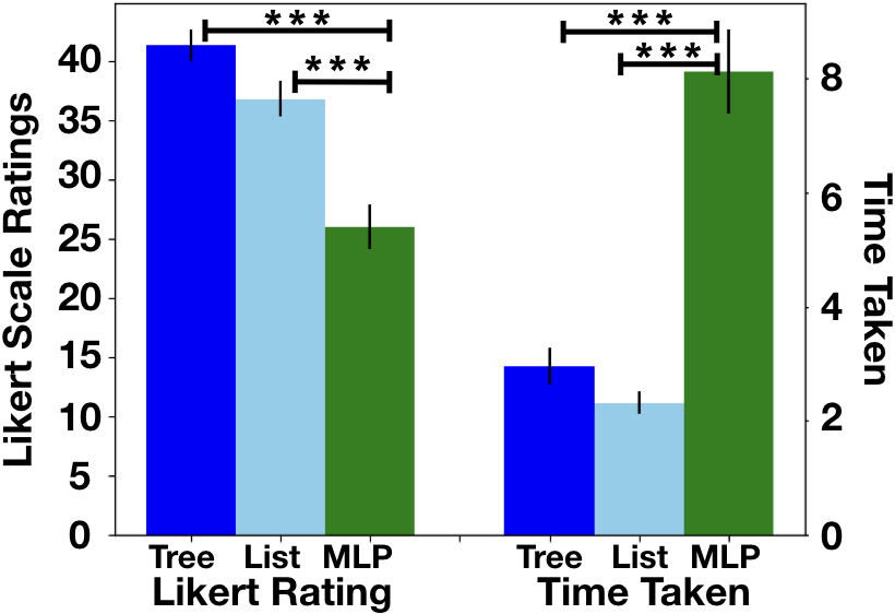
7.2 Study Results
Results of our study are shown in Figure 7. We perform an ANOVA and find that the type of decision-making aid had a statistically significant effect on users’ Likert scale ratings for usability and interpretability (). We test for normality and homoscedasticity and do not reject the null hypothesis in either case, using Shapiro-Wilk () and Levene’s Test (), respectively. A Tukey’s HSD post-hoc test shows that the tree (, ) and decision list (, ) both rated significantly higher than a one-hot MLP.
We also test the time participants took to use each decision-making aid for a set of five prompts. We applied Friedman’s test and found the type of aid had a significant effect on completion time (). Dunn’s test showed that the tree (, ) and decision list (, ) times were statistically significantly shorter than the one-hot MLP completion times.
We note that participants were shown the full MLP after the questionnaire’s conclusion, and participants consistently reported they would have abandoned the task if they had been presented with a full MLP as their aid. These results support the hypothesis that decision trees and lists are significantly superior decision-making aids in reducing human frustration and increasing efficiency. This study, coupled with our strong performance results over MLPs, shows the power of our approach to interpretable, online RL via DDTs.
8 Future Work
We propose investigating how our framework could leverage advances in other areas of deep learning, e.g. inferring feature embeddings. For example, we could learn subject-specific embeddings via backpropagation but within an interpretable framework for personalized medicine (Killian et al., 2017) or in apprenticeship learning (Gombolay et al., 2018b), particularly when heterogeneity precludes a one-size-fits-all model (Chen et al., 2020). We could also invert our learning process to a prior specify a decision tree policy given expert knowledge, which we could then train via policy gradient (Silva and Gombolay, 2019).
9 Conclusion
We demonstrate that DDTs can be used in RL to generate interpretable policies. We provide a motivating analysis showing the benefit of using policy gradients to train DDTs in RL challenges over Q-learning. This analysis serves to guide researchers and practitioners alike in future research and application of DDTs to learn interpretable RL policies. We show that DDTs trained with policy gradient can provide comparable and even superior performance against MLP baselines. Finally, we conduct a user study which demonstrates that DDTs and decision lists offer increased interpretability and usability over MLPs while also taking less time and providing efficient insight into policy behavior.
10 Acknowledgements
This work was funded by the Office of Naval Research under grant N00014-19-1-2076 and by MIT Lincoln Laboratory under grant # MIT Lincoln Laboratory grant 7000437192.
References
- Andrychowicz et al. [2016] Marcin Andrychowicz, Misha Denil, Sergio Gomez, Matthew W Hoffman, David Pfau, Tom Schaul, Brendan Shillingford, and Nando De Freitas. Learning to learn by gradient descent by gradient descent. In Advances in Neural Information Processing Systems, pages 3981–3989, 2016.
- Andrychowicz et al. [2018] Marcin Andrychowicz, Bowen Baker, Maciek Chociej, Rafal Jozefowicz, Bob McGrew, Jakub Pachocki, Arthur Petron, Matthias Plappert, Glenn Powell, Alex Ray, et al. Learning dexterous in-hand manipulation. arXiv preprint arXiv:1808.00177, 2018.
- Angelino et al. [2017] Elaine Angelino, Nicholas Larus-Stone, Daniel Alabi, Margo Seltzer, and Cynthia Rudin. Learning certifiably optimal rule lists for categorical data. The Journal of Machine Learning Research, 18(1):8753–8830, 2017.
- Arulkumaran et al. [2017] Kai Arulkumaran, Mark Peter Deisenroth, Miles Brundage, and Anil Anthony Bharath. A brief survey of deep reinforcement learning. IEEE Signal Processing Magazine, 34(6):26–38, 2017.
- Baird [1995] Leemon Baird. Residual algorithms: Reinforcement learning with function approximation. In Machine Learning Proceedings 1995, pages 30–37. Elsevier, 1995.
- Bertsekas and Tsitsiklis [1996] Dimitri P Bertsekas and John N Tsitsiklis. Neuro-dynamic programming, volume 5. Athena Scientific Belmont, MA, 1996.
- Bottou [2010] Léon Bottou. Large-scale machine learning with stochastic gradient descent. In Proceedings of COMPSTAT’2010, pages 177–186. Springer, 2010.
- Breiman et al. [1984] Leo Breiman, Jerome Friedman, Charles Stone, and Richard Olshen. Classification and regression trees. CRC press, 1984.
- Brockman et al. [2016] Greg Brockman, Vicki Cheung, Ludwig Pettersson, Jonas Schneider, John Schulman, Jie Tang, and Wojciech Zaremba. Openai gym, 2016.
- Chen and Rudin [2017] Chaofan Chen and Cynthia Rudin. An optimization approach to learning falling rule lists. arXiv preprint arXiv:1710.02572, 2017.
- Chen et al. [2020] Letian Chen, Rohan Paleja, Muyleng Ghuy, and Matthew Gombolay. Joint goal and strategy inference across heterogeneous demonstrators via reward network distillation. In Proceedings of the International Conference on Human-Robot Interaction, 2020.
- Doshi-Velez and Kim [2017] Finale Doshi-Velez and Been Kim. Towards a rigorous science of interpretable machine learning. arXiv preprint arXiv:1702.08608, 2017.
- Ernst and Wehenkel [2005] Pierre Geurts Ernst, Damien and Louis Wehenkel. Tree-based batch mode reinforcement learning. Journal of Machine Learning Research, 6(Apr):503–556, 2005.
- Espeholt et al. [2018] Lasse Espeholt, Hubert Soyer, Remi Munos, Karen Simonyan, Volodymir Mnih, Tom Ward, Yotam Doron, Vlad Firoiu, Tim Harley, Iain Dunning, et al. Impala: Scalable distributed deep-rl with importance weighted actor-learner architectures. arXiv preprint arXiv:1802.01561, 2018.
- Finney [2002] Gardiol Natalia H. Kaelbling Leslie Pack Oates Tim Finney, Sara. The thing that we tried didn’t work very well: deictic representation in reinforcement learning. In Proceedings of the Conference on Uncertainty in Artificial Intelligence, pages 154–161. Morgan Kaufmann Publishers Inc., 2002.
- Finney [1998] Mark A Finney. Farsite: Fire area simulator-model development and evaluation. Res. Pap. RMRS-RP-4, Revised 2004. Ogden, UT: US Department of Agriculture, Forest Service, Rocky Mountain Research Station. 47 p., 4, 1998. URL https://www.fs.fed.us/rm/pubs/rmrs_rp004.pdf.
- Fletcher and Powell [1963] Roger Fletcher and Michael JD Powell. A rapidly convergent descent method for minimization. The computer journal, 6(2):163–168, 1963.
- Gawande [2010] Atul Gawande. Checklist Manifesto, The (HB). Penguin Books India, 2010.
- Gombolay et al. [2018a] Matthew Gombolay, Reed Jensen, Jessica Stigile, Toni Golen, Neel Shah, Sung-Hyun Son, and Julie Shah. Human-machine collaborative optimization via apprenticeship scheduling. Journal of Artificial Intelligence Research, 63:1–49, 2018a.
- Gombolay et al. [2018b] Matthew Gombolay, Xi Jessie Yang, Bradley Hayes, Nicole Seo, Zixi Liu, Samir Wadhwania, Tania Yu, Neel Shah, Toni Golen, and Julie Shah. Robotic assistance in the coordination of patient care. The International Journal of Robotics Research, 37(10):1300–1316, 2018b.
- Gordon [1995] Geoffrey J Gordon. Stable function approximation in dynamic programming. In Machine Learning Proceedings 1995, pages 261–268. Elsevier, 1995.
- Haksar and Schwager [2018] Ravi N Haksar and Mac Schwager. Distributed deep reinforcement learning for fighting forest fires with a network of aerial robots. In 2018 IEEE/RSJ International Conference on Intelligent Robots and Systems (IROS), pages 1067–1074. IEEE, 2018.
- Haynes [2009] Thomas G. Weiser William R. Berry Stuart R. Lipsitz Abdel-Hadi S. Breizat E. Patchen Dellinger Teodoro Herbosa et al. Haynes, Alex B. A surgical safety checklist to reduce morbidity and mortality in a global population. New England Journal of Medicine, 360(5):491–499, 2009.
- Killian et al. [2017] Taylor W Killian, Samuel Daulton, George Konidaris, and Finale Doshi-Velez. Robust and efficient transfer learning with hidden parameter markov decision processes. In Advances in Neural Information Processing Systems, pages 6250–6261, 2017.
- Kostrikov [2018] Ilya Kostrikov. Pytorch implementations of reinforcement learning algorithms. https://github.com/ikostrikov/pytorch-a2c-ppo-acktr, 2018.
- Lakkaraju and Rudin [2017] Himabindu Lakkaraju and Cynthia Rudin. Learning cost-effective and interpretable treatment regimes. In Artificial Intelligence and Statistics, pages 166–175, 2017.
- Letham et al. [2015] Benjamin Letham, Cynthia Rudin, Tyler H McCormick, David Madigan, et al. Interpretable classifiers using rules and bayesian analysis: Building a better stroke prediction model. The Annals of Applied Statistics, 9(3):1350–1371, 2015.
- Lipton [2018] Zachary C Lipton. The mythos of model interpretability. Queue, 16(3):31–57, 2018.
- Mnih et al. [2013] Volodymyr Mnih, Koray Kavukcuoglu, David Silver, Alex Graves, Ioannis Antonoglou, Daan Wierstra, and Martin Riedmiller. Playing atari with deep reinforcement learning. arXiv preprint arXiv:1312.5602, 2013.
- Natarajan and Gombolay [2020] Manisha Natarajan and Matthew Gombolay. Effects of anthropomorphism and accountability on trust in human robot interaction. In Proceedings of the International Conference on Human-Robot Interaction, 2020.
- Pedregosa [2011] Gaël Varoquaux Alexandre Gramfort Vincent Michel Bertrand Thirion Olivier Grisel Mathieu Blondel et al. Pedregosa, Fabian. Scikit-learn: Machine learning in Python. Journal of Machine Learning Research, 12:2825–2830, 2011.
- Pyeatt and Howe [2001] Larry D. Pyeatt and Adele E. Howe. Decision tree function approximation in reinforcement learning. In Proceedings of the third international symposium on adaptive systems: evolutionary computation and probabilistic graphical models, volume 2, pages 70–77. Cuba, 2001.
- Rajeswaran et al. [2017] Aravind Rajeswaran, Vikash Kumar, Abhishek Gupta, Giulia Vezzani, John Schulman, Emanuel Todorov, and Sergey Levine. Learning complex dexterous manipulation with deep reinforcement learning and demonstrations. arXiv preprint arXiv:1709.10087, 2017.
- Rudin [2014] Cynthia Rudin. Algorithms for interpretable machine learning. In Proceedings of the ACM SIGKDD International Conference on Knowledge Discovery and Data Mining, pages 1519–1519. ACM, 2014.
- Schulman et al. [2017] John Schulman, Filip Wolski, Prafulla Dhariwal, Alec Radford, and Oleg Klimov. Proximal policy optimization algorithms, 2017.
- Serrano and Smith [2019] Sofia Serrano and Noah A Smith. Is attention interpretable? arXiv preprint arXiv:1906.03731, 2019.
- Shah and Gopal [2010] Hitesh Shah and Madan Gopal. Fuzzy decision tree function approximation in reinforcement learning. International Journal of Artificial Intelligence and Soft Computing, 2(1-2):26–45, 2010.
- Silva and Gombolay [2019] Andrew Silva and Matthew Gombolay. Prolonets: Neural-encoding human experts’ domain knowledge to warm start reinforcement learning. arXiv preprint arXiv:1902.06007, 2019.
- Silver [2016] Aja Huang Chris J. Maddison Arthur Guez Laurent Sifre George Van Den Driessche Julian Schrittwieser et al. Silver, David. Mastering the game of go with deep neural networks and tree search. Nature, 529(7587):484–489, 2016.
- Suárez and Lutsko [1999] Alberto Suárez and James F Lutsko. Globally optimal fuzzy decision trees for classification and regression. IEEE Transactions on Pattern Analysis and Machine Intelligence, 21(12):1297–1311, 1999.
- Sun et al. [2018] Peng Sun, Xinghai Sun, Lei Han, Jiechao Xiong, Qing Wang, Bo Li, Yang Zheng, Ji Liu, Yongsheng Liu, Han Liu, et al. Tstarbots: Defeating the cheating level builtin ai in starcraft ii in the full game. arXiv preprint arXiv:1809.07193, 2018.
- Sutton and Mansour [2000] David A. McAllester Satinder P. Singh Sutton, Richard S. and Yishay Mansour. Policy gradient methods for reinforcement learning with function approximation. In NIPS, pages 1057–1063, 2000.
- Sutton and Barto [1998] Richard S. Sutton and Andrew G. Barto. Reinforcement learning: An introduction. MIT Press, 1998.
- Tieleman and Hinton [2012] Tijmen Tieleman and Geoffrey Hinton. Lecture 6.5-rmsprop: Divide the gradient by a running average of its recent magnitude. COURSERA: Neural networks for machine learning, 4(2):26–31, 2012.
- Tsitsiklis and Van Roy [1996] John N Tsitsiklis and Benjamin Van Roy. Feature-based methods for large scale dynamic programming. Machine Learning, 22(1-3):59–94, 1996.
- Vinyals et al. [2017] Oriol Vinyals, Timo Ewalds, Sergey Bartunov, Petko Georgiev, Alexander Sasha Vezhnevets, Michelle Yeo, Alireza Makhzani, Heinrich Küttler, John Agapiou, Julian Schrittwieser, et al. Starcraft ii: A new challenge for reinforcement learning. arXiv preprint arXiv:1708.04782, 2017.
- Voigt and Von dem Bussche [2017] Paul Voigt and Axel Von dem Bussche. The eu general data protection regulation (gdpr). A Practical Guide, 1st Ed., Cham: Springer International Publishing, 2017.
- Watkins [1989] Christopher John Cornish Hellaby Watkins. Learning from delayed rewards. PhD thesis, King’s College, Cambridge, 1989.
- Weiss and Indurkhya [1995] Sholom M. Weiss and Nitin Indurkhya. Rule-based machine learning methods for functional prediction. Journal of Artificial Intelligence Research, 3:383–403, 1995.
- Zhang et al. [2019] Quanshi Zhang, Yu Yang, Haotian Ma, and Ying Nian Wu. Interpreting cnns via decision trees. In Proceedings of the IEEE Conference on Computer Vision and Pattern Recognition, pages 6261–6270, 2019.
Appendix A: Derivation of the Optimal Policy
In this section, we provide a derivation of the optimal policy for the MDP in Fig. 1(b). For this derivation, we use the definition of the Q-function described in Eq. 18, where is the state resulting from applying action in state . In keeping with the investigation in this paper, we assume deterministic transitions between states (i.e., from Eq. 17). As such, we can ignore and simply apply Eq. 19.
| (17) |
| (18) | ||||
| (19) |
Theorem 1
We begin by asserting in Eq. 20 that the Q-values for are given and for any action . This result is due to the definition that states and are terminal states and the reward for those states is regardless of the action applied. We note that, in our example, , but we leave it here for the sake of generality.
| (20) |
Next, we must compute the Q-values for the remaining state-action pairs, as shown in Eq. 21-24.
| (21) | ||||
| (22) | ||||
| (23) | ||||
| (24) |
By the definition of the MDP in Fig. 8, we substitute in for as shown in Eq. 25-28.
| (29) | ||||
| (30) |
For the Q-value of state-action pair, , we must determine whether is less than or equal to . If the agent were to apply action in state , we can see from Eq. 30 that the agent would receive at a minimum , because , must be the maximum from Eq. 29. We can make a symmetric argument for in Eq. 30. Given this relation, we arrive at Eq. 31 and 32.
| (31) | ||||
| (32) |
Eq. 31 and 32 represent a recursive, infinite geometric series, as depicted in Eq. 34.
| (33) | ||||
| (34) |
In the case that , Eq. 34 represents an infinite geometric series, the solution to which is . In our case however, (i.e., four-time steps). As such, , as shown in Eq. 35.
| (35) |
Recall that given our definition of the MDP in Fig. 8. Therefore, . If the RL agent is non-myopic, i.e., , then we have the strict inequality . For these non-trivial settings of , we can see that the optimal policy for the RL agent is to apply action in state and action in state . Lastly, because and are terminal states, the choice of action is irrelevant, as seen in Eq. 20.
The optimal policy is then given by Eq. 36.
| (36) |
Appendix B: Policy Traces and Value
This section reports the execution traces and corresponding value calculations of a Boolean decision treee with varying for the simple MDP model from Figure 8.
Appendix C: Q-learning Leaf Values
| Leaf | Q-function | Eq. | Q-value |
|---|---|---|---|
| Eq. 26 | |||
| Eq. 27 | |||
| Eq. 35 | |||
| Eq. 35 |
For the decision tree in Fig. 9, there are four leaf values: , , , and . Table 4 contains the settings of those parameters. In Table 4, the first column depicts the leaf parameters; the second column depicts the Q-function state-action pair; the third column contains the equation reference to Appendix A, where the Q-value is calculated; and the fourth column contains the corresponding Q-value. These Q-values assume that the agent begins in a non-terminal state (i.e., or ) and follows the optimal policy represented by Eq. 36.
Appendix D: Probability of Incorrect Action
| (37) |
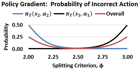
The output of the differentiable tree is a weighted, nonlinear combination of the leaves (Eq. 37). Using PG, one samples actions probabilistically from . The probability of applying the “wrong” action (i.e., one resulting in a negative reward) is in state and in state . Assuming it equally likely to be in states and , the overall probability is . These probabilities are depicted in Fig. 10, which shows how the optimal setting, , for should be using PG.
Appendix E: Architecture Sweeps
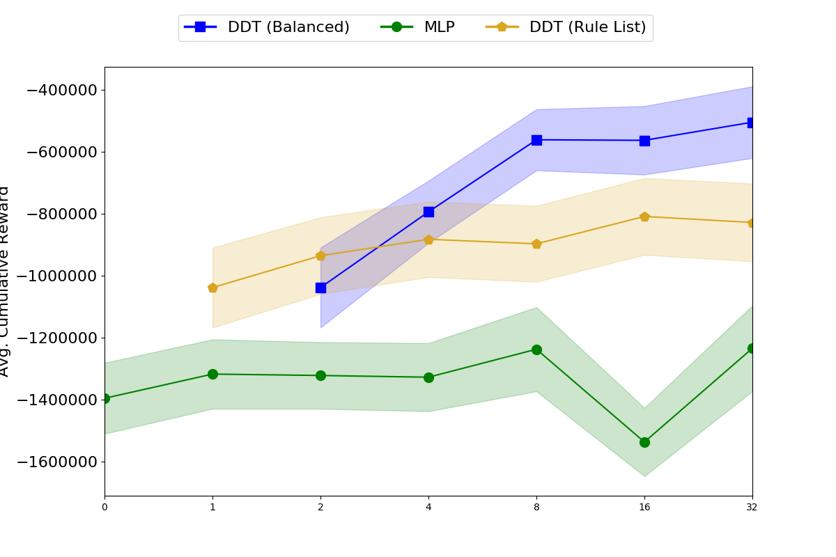
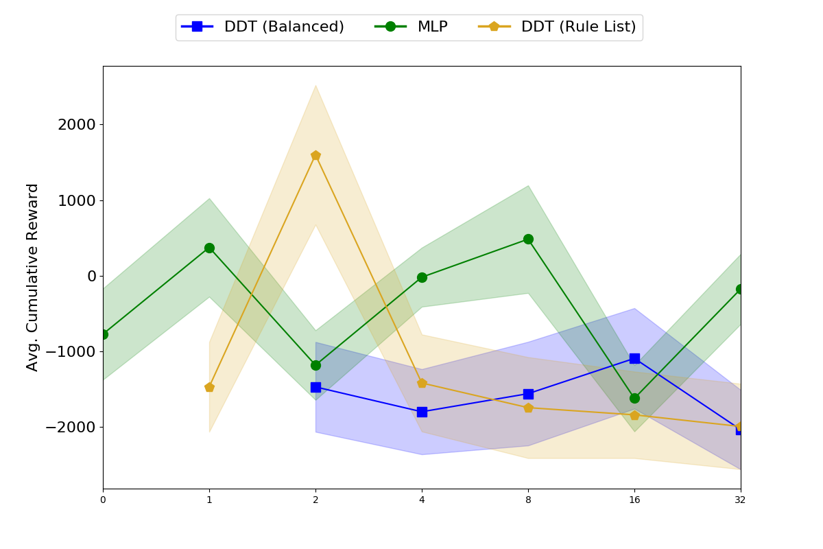
We performed architecture sweeps, as mentioned in the main paper, across all types of models. We found that the MLP requires small models for simple domains, the DDT methods are all relatively unaffected by increased depth, representing a benefit of applying DDTs to various RL tasks. For this result, see Figure 11. As shown in Figure 12, in more complex domains, the results are less conclusive and increased depth does not show clear trends for any approach. Nonetheless, we show evidence that DDTs are at least competitive with MLPs for RL tasks of varying complexity, and that they are more robust to hyperparameter tuning with respect to depth and number of layers.
We find that the MLP with no hidden layers performs the best on the two OpenAI Gym domains, cart pole and lunar lander. The best differentiable decision tree architectures for the cart pole domain are those with two leaves and two rules, while the best architectures for lunar lander include 32 leaves and 16 rules.
In the wildfire tracking domain, the 8-layer MLP performed the best of the MLPs, while the 32-leaf differentiable decision tree was the top differentiable decision tree, and the 32-rule differentiable rule list performed the best of the differentiable rule lists.
Finally, the MLP in the FindAndDefeatZerglings domain is an 8-layer MLP, and the differentiable decision tree uses 8 leaves while the differentiable rule list uses 8 rules.
MLP hidden layer sizes preserve the input data dimension through all hidden layers until finally downsampling to the action space for the final layer. MLP networks all use the ReLU activation after it performed best in a hyperparameter sweep.
Appendix F: Domain Details
.1 Wildfire Tracking
The wildfire tracking domain input space is:
-
•
Fire 1 Distance North (float)
-
•
Fire 1 Distance West (float)
-
•
Closest To Fire 1 (Boolean)
-
•
Fire 2 Distance North (float)
-
•
Fire 2 Distance West (float)
-
•
Closest To Fire 2 (Boolean)
Distance features are floats, representing how far north or west the fire is, relative to the drone. Distances can also be negative, implying that the fire is south or east of the drone.
.2 StarCraft II Micro-battle Evaluation
The FindAndDefeatZerglings manufactured input space is:
-
•
X Distance Away (float)
-
•
Y Distance Away (float)
-
•
Percent Health Remaining (float)
-
•
Percent Weapon Cooldown Remaining (float)
for each agent-controlled unit and 2 allied units, as well as:
-
•
X Distance Away (float)
-
•
Y Distance Away (float)
-
•
Percent Health Remaining (float)
-
•
Percent Weapon Cooldown Remaining (float)
-
•
Enemy Unit Type (Boolean)
for the five nearest enemy units. Missing data is filled in with . The action space for this domain consists of:
-
•
Move North
-
•
Move East
-
•
Move West
-
•
Move South
-
•
Attack Nearest Enemy
-
•
Attack Second Nearest Enemy
-
•
Attack Third Nearest Enemy
-
•
Attack Second Farthest Enemy
-
•
Attack Farthest Enemy
-
•
Do Nothing
Interpretable Policies
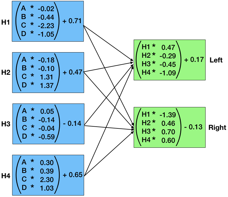
Here we include interpretable policies for each domain, without the pruning that is included in versions in the main body. See Fig. 13, 14, 15, and 16. Finally, we also include examples of two MLPs represented as decision-making aids. The first is the one-hot MLP that was given to study participants for evaluation of interpretability and efficiency, shown in Figure 17. The second is the true cart pole MLP, available in Figure 18. This decision-making aid turned out to be exceptionally complicated, even with no activation functions and no hidden layer.
Sample Survey Questions
Survey questions included Likert scale questions ranging from 1 (Very Strongly Disagree) to 7 (Very Strongly Agree). For both the MLP and decision trees, some questions included:
-
1.
I understand the behavior represented within the model.
-
2.
The decision-making process does not make sense.
-
3.
The model’s logic is easy to follow
-
4.
I like the level of readability of this model.
-
5.
The model is difficult to understand.