Unidirectional Maxwellian Spin Waves

Abstract

We develop a unified perspective of unidirectional topological edge waves in non-reciprocal media. We focus on the inherent role of photonic spin in non-reciprocal gyroelectric media, ie. magnetized metals or magnetized insulators. Due to the large body of contradicting literature, we point out at the outset that these Maxwellian spin waves are fundamentally different from well-known topologically trivial surface plasmon polaritons (SPPs). We first review the concept of a Maxwell Hamiltonian in non-reciprocal media, which immediately reveals that the gyrotropic coefficient behaves as a photon mass in two dimensions. Similar to the Dirac mass, this photonic mass opens bandgaps in the energy dispersion of bulk propagating waves. Within these bulk photonic bandgaps, three distinct classes of Maxwellian edge waves exist - each arising from subtle differences in boundary conditions. On one hand, the edge wave solutions are rigorous photonic analogs of Jackiw-Rebbi electronic edge states. On the other hand, for the exact same system, they can be high frequency photonic counterparts of the integer quantum Hall effect, familiar at zero frequency. Our Hamiltonian approach also predicts the existence of a third distinct class of Maxwellian edge wave exhibiting topological protection. This occurs in an intriguing topological bosonic phase of matter, fundamentally different from any known electronic or photonic medium. The Maxwellian edge state in this unique quantum gyroelectric phase of matter necessarily requires a sign change in gyrotropy arising from non-locality (spatial dispersion). In a Drude system, this behavior emerges from a spatially dispersive cyclotron frequency that switches sign with momentum. A signature property of these topological electromagnetic edge states is that they are oblivious to the contacting medium, ie. they occur at the interface of the quantum gyroelectric phase and any medium (even vacuum). This is because the edge state satisfies open boundary conditions - all components of the electromagnetic field vanish at the interface. Furthermore, the Maxwellian spin waves exhibit photonic spin-1 quantization in exact analogy with their supersymmetric spin-$\nicefrac{{1}}{{2}}$ counterparts. The goal of this paper is to discuss these three foundational classes of edge waves in a unified perspective while providing in-depth derivations, taking into account non-locality and various boundary conditions. Our work sheds light on the important role of photonic spin in condensed matter systems, where this definition of spin is also translatable to topological photonic crystals and metamaterials.

I Introduction

Gyroelectric media, or magnetized plasmas, form the canonical system to study non-reciprocity Mackay and Lakhtakia (2016); Caloz et al. (2018); Mirmoosa et al. (2014); Valente et al. (2015); Floess and Giessen (2018); Zyuzin (2017). There has been recent interest in such media for their potential to break the time-bandwidth limit inside cavities Mann et al. (2019); Tsakmakidis et al. (2017), sub-diffraction imaging Zhang et al. (2011), unique absorption Green (2012) and thermal properties Zhu and Fan (2016), and for one-way topological transitions Leviyev et al. (2017). It should be emphasized that the gyroelectric coefficient ($g$), which embodies antisymmetric components of the permittivity tensor ($\varepsilon_{ij}$), is intimately related to its low frequency counterpart in condensed matter physics - the transverse Hall conductivity ($\sigma_{H}=\sigma_{xy}=-i\omega g$) Stern (2008); Vandendriessche et al. (2012). The goal of this paper is to bridge the gap between modern concepts in nanophotonics, magnetized plasma physics, and condensed matter physics.

Historically, gyroelectric media was popularized in plasma physics Landau et al. (1975, 2013) where the “gyration vector” or “rotation axis” sets a preferred handedness to the medium. This causes non-reciprocal (direction dependent) wave propagation along the axis of the medium. The non-reciprocal properties are now well understood but only recently has the connection with the Dirac equation been revealed Van Mechelen and Jacob (2018a, b); Mechelen and Jacob (2019); Horsley (2018); Bialynicki-Birula and Bialynicka-Birula (2013); Barnett (2014); Horsley (2018). This immediately leads to multiple new insights related to energy density, photon spin and photon mass for wave propagation within two-dimensional gyrotropic media Van Mechelen and Jacob (2018b); Mechelen and Jacob (2019); Horsley (2018); Dunne (1999). In particular, a unique phenomenon related to gyrotropic media is the presence of unidirectional edge waves, fundamentally different from surface plasmon polaritons (SPPs) or Dyakonov waves Prudêncio and Silveirinha (2018); Davoyan and Engheta (2013). We note that photonic crystals Lu et al. (2016); Shalaev et al. (2018); Noh et al. (2018) or metamaterials Khanikaev and Shvets (2017); Chang et al. (2017); Lin et al. (2018) are not necessary for this phenomenon and even a continuous medium (eg: magnetized plasma or doped semiconductor) can host unidirectional edge waves.

The role of spin has not been revealed till date but chiral (unidirectional) photonic waves in gyrotropic media have a rich history. Early work introduced the concept of optical isomers Zhukov and Raikh (2000) which is the interface of two gyrotropic media with opposite signs of non-reciprocal coefficients (half-space of $g>0$ interfaced with another half-space of $g<0$). It was shown that unique chiral edge states emerge, addressed as the “quantum Cotton-Mouton effect”, which are similar in nature to the electronic quantum Hall effect. These chiral edge states were also predicted on the interface of Weyl semimetals Zyuzin and Zyuzin (2015). Raghu and Haldane’s original model to realize a one-way waveguide dealt with the gyroelectric photonic crystals Haldane and Raghu (2008); Raghu and Haldane (2008). More recently, gyroelectric magneto-plasmons have been demonstrated in quantum well structures under biasing magnetic fields Jin et al. (2016); Mahoney et al. (2017). Another important example of unidirectional edge waves occurs when a gyrotropic medium is terminated with a perfect electric conductor (PEC), as shown by Silveirinha Lannebère and Silveirinha (2018). Horsley Horsley (2018) recently proved that this PEC boundary is equivalent to antisymmetric solutions of optical isomers (two gyrotropic media with opposite signs $\pm g$) and leads to unidirectional Jackiw-Rebbi type photonic waves.

However, in all the above examples, the electromagnetic boundary conditions are drastically different from the open boundary conditions utilized for topologically-protected solutions of the Dirac equation Delplace et al. (2011); Mong and Shivamoggi (2011); Shen et al. (2011); Shen (2017); Medhi and Shenoy (2012); Bernevig and Hughes (2013). This challenge was recently overcome when a Dirac-Maxwell correspondence was applied to gyrotropic media Van Mechelen and Jacob (2018b); Mechelen and Jacob (2019), which derived the supersymmetric (spin-1) partner of the topological Dirac equation. This framework gave rise to a new unidirectional edge wave with open boundary conditions, such that the electromagnetic field completely vanishes at the material interface Van Mechelen and Jacob (2018b); Mechelen and Jacob (2019). The necessary conditions for the existence of such a wave is non-reciprocity $g$, temporal dispersion $g(\omega)$, and spatial dispersion $g(\omega,k)$. A momentum dependent sign change in the gyrotropic coefficient $g(\omega,k_{\mathrm{crit}})=0$ leads to a topologically nontrivial electromagnetic field - a quantum gyroelectric phase of matter. In Drude systems, this corresponds to a momentum dependent sign change of the cyclotron frequency. It should be emphasized that this topological phase of matter is Maxwellian (spin-1 bosonic) and is unlike any known spin-$\nicefrac{{1}}{{2}}$ fermionic phases of matter (eg: graphene, Chern insulator, etc.). The unidirectional photonic edge wave is a fundamental mode of this nonlocal, non-reciprocal medium and cannot be separated from the bulk. The contacting medium has no influence on the edge wave, unlike the previously mentioned examples which are sensitive to boundary conditions. We address this phenomenon as the quantum gyroelectric effect (QGEE) and it remains an open question whether such a Maxwellian phase of matter can be found in nature.

The purpose of this paper is to present the first unified view of all the aforementioned unidirectional edge waves in non-reciprocal media. The essence of our results is captured in Fig. 1 and Tab. 1 which contrasts unidirectional edge waves of the quantum gyroelectric effect (QGEE), photonic quantum Hall (PQH) states and photonic Jackiw-Rebbi (PJR) states. All such waves appear in gyroelectric media but boast surprisingly different behavior. The QGEE displays bulk-boundary correspondence Mong and Shivamoggi (2011) since it is defined independent of the contacting medium [Sec. IV]. The PQH states host a high frequency quantum Hall edge current which arises from a discontinuity in the electromagnetic field [Sec. VI]. Lastly, the PJR edge waves are domain wall states [Sec. VII]. Another important result of our paper is illustrated in Fig. 2 which shows that the two classes of unidirectional waves, PQH and PJR, can be realized at perfect magnetic conductor (PMC) and perfect electric conductor (PEC) boundary conditions respectively.

This article is organized as follows. Sec. II presents an overview of spin waves. In Sec. III and IV we show that a nonlocal, non-reciprocal medium is foundational to the concept of 2+1D topological phases of matter. We review the concept of Dirac-Maxwell correspondence which can be exploited to introduce a Hamiltonian for light within complex photonic media. This framework allows us to rigorously define helicity and spin while also identifying a photonic mass, which is directly proportional to the gyrotropic coefficient. We then discuss the necessity of temporally and spatially dispersive optical response parameters to define electromagnetic topological invariants for bulk continuous media. Although commonly ignored, nonlocality is absolutely essential for the electromagnetic theory to be consistent with the tenfold way Ryu et al. (2010), which describes all possible continuum topological phases, in every dimension. In the topologically nontrivial regime $C\neq 0$, the unidirectional Maxwellian spin wave is derived and satisfies open boundary conditions - this is the QGEE. Following these results, we analyze the interface of optical isomers [Sec. V] and derive the photonic quantum Hall [Sec. VI] and photonic Jackiw-Rebbi edge states [Sec. VII]. The final Sec. VIII presents our conclusions.

II Overview of spin waves

We outline the key properties of chiral Maxwellian spin waves which, surprisingly, emerge in two distinct physical systems. First, it is identified in the low momentum dispersion of the QGEE. Second, it also represents the photonic counterpart of the Jackiw-Rebbi domain wall state known in the continuum Dirac equation Shen et al. (2011); Shen (2017); Jackiw and Rebbi (1976); Schuster et al. (2016). The Dirac Jackiw-Rebbi wave exists at the interface of inverted masses, $\Lambda>0$ and $\Lambda<0$, and is an eigenstate of the spin-$\nicefrac{{1}}{{2}}$ helicity (Pauli) operator. The exact parallel in photonics can now be established as it has been proven that gyrotropy plays the role of photonic mass. Thus, a unique Maxwellian spin wave exists at the interface of optical isomers, $g>0$ and $g<0$. Furthermore, this electromagnetic wave is an eigenstate of the SO(3) operator (spin-1 helicity operator) and exhibits helical quantization. This is intuitively clear since the edge wave is purely transverse electro-magnetic (TEM); the polarization is orthogonal to the momentum $\hat{k}\cdot\vec{E}=0$.

To avoid confusion, we contrast between conventional surface plasmon polaritons (SPPs) and Maxwellian spin waves which both display spin-momentum locking phenomena but in fundamentally different forms. Even SPPs on magnetized plasmas do not show the same characteristics as chiral Maxwellian spin waves as they are not eigenstates of the SO(3) vector operators. We strongly emphasize that SPPs on conventional (electric) metals, magnetic metals, as well as negative index media Smith et al. (2004) do not possess any topological characteristics. There exists no bulk-boundary correspondence as the bulk media are trivial. Spin-momentum locking in these redsurface waves is transverse and not quantized Mechelen and Jacob (2016); Kalhor et al. (2016); Bliokh et al. (2015a); Mitsch et al. (2014); Young et al. (2015); Bliokh et al. (2015b); Lodahl et al. (2017); Picardi et al. (2018). This means the spin is perpendicular to the momentum and is a continuous (classical) number. On the contrary, spin-momentum locking arising in Maxwellian spin waves is longitudinal and quantized. This means the spin is parallel to the momentum and is a discrete (quantum) number, assuming values of $\pm 1$ only. Despite recent observations of spin-momentum locking phenomena in waveguides Kapitanova et al. (2014); Luo et al. (2017), resonators Wang et al. (2019) and surface plasmon polaritons Lin et al. (2013), no wave has been discovered to be a pure spin state with quantized eigenvalues of the helicity operator. Our work is an answer to this endeavor.

As an aside, we must also point out that orbital angular momentum (OAM) quantization for photons is unrelated to topological quantization Carroll et al. (2004), such as Chern number quantization. OAM quantization is routinely encountered for classical optical waves in free-space beams Gawhary et al. (2018), microdisk resonators, optical fibers, whispering gallery mode resonators Yao and Padgett (2011), etc. The origin of topological quantization is always a singularity/discontinuity in the underlying gauge potential Wu and Yang (1976); Rajantie (2012); Fang et al. (2003). This phenomenon of gauge singularity/discontinuity has been proven to occur in the Berry connection of the quantum gyroelectric phase Van Mechelen and Jacob (2018b); Mechelen and Jacob (2019). Nevertheless, it remains an open question whether such topological quantization is connected to physical observables (response/correlation functions) of the photon, like they are for the electron. For example, quantization of the Hall conductivity $\sigma_{H}$ was the first striking experimental observable connected to topology Hatsugai (1993, 1997). No photonic equivalent is known to date.

Figure 1: (a), (b) and (c) are schematics of the quantum gyroelectric effect (QGEE), photonic quantum Hall (PQH) and photonic Jackiw-Rebbi (PJR) edge states respectively. The characteristic spatial profile of $E_{x}(x)$ is displayed for each edge state along with the corresponding boundary conditions. (a) The QGEE is a topologically-protected unidrectional (chiral) edge state and exists at the boundary of any medium - even vacuum. The QGEE is fundamentally tied to nonlocal (spatially dispersive) gyrotropy $g(\omega,k)$ and can never be realized in a purely local model. (b) The PQH edge state is the photonic analogue of the quantum Hall effect and hosts a high-frequency edge current $I_{y}$. The presence of the edge current $I_{y}\neq 0$ creates a discontinuity in the fields across the boundary, $E_{x}(0^{-})\neq E_{x}(0^{+})$ and $H_{z}(0^{-})\neq H_{z}(0^{+})$. (c) The PJR edge state is the photonic equivalent of the inverted mass problem arising in the Dirac equation. This state possesses no edge current $I_{y}=0$ and is completely transverse electro-magnetic (TEM) as the longitudinal field vanishes entirely $E_{y}(x)=0$.

III Maxwell Hamiltonian

III.1 Vacuum

Before defining Maxwellian spin waves [Fig. 1], that emerge at the boundaries of matter, we illustrate the direct correspondence of spin operators arising in Maxwell’s equations and the massless Dirac equation in 2+1D. We will then show that this correspondence extends to massive particles in Sec. III.3. In two spatial dimensions we can focus strictly on transverse-magnetic (TM) waves, where the magnetic field $H_{z}$ is perpendicular to the plane of propagation $\mathbf{k}=k_{x}\hat{x}+k_{y}\hat{y}$. Maxwell’s equations in the reciprocal momentum space $\mathcal{H}_{0}(\mathbf{k})$ are expressed compactly as Van Mechelen and Jacob (2018b); Mechelen and Jacob (2019); Horsley (2018),

$$\mathcal{H}_{0}(\mathbf{k})f=\omega f,\qquad f=\begin{bmatrix}E_{x}\\ E_{y}\\ H_{z}\end{bmatrix}.$$ (1)

$f$ is the TM polarization of the electromagnetic field and is operated on by the free-space “Maxwell Hamiltonian”,

$$\mathcal{H}_{0}(\mathbf{k})=\begin{bmatrix}0&0&-k_{y}\\ 0&0&k_{x}\\ -k_{y}&k_{x}&0\end{bmatrix}=k_{x}\hat{S}_{x}+k_{y}\hat{S}_{y}.$$ (2)

Maxwell’s equations describe optical helicity, ie. the projection of the momentum $\mathbf{k}$ onto the spin $\vec{S}$. In this case, $\hat{S}_{x}$ and $\hat{S}_{y}$ are spin-1 operators that satisfy the angular momentum algebra $[\hat{S}_{i},\hat{S}_{j}]=i\epsilon_{ijk}\hat{S}_{k}$. These operators are expressed in matrix form as,

$$\hat{S}_{x}=\begin{bmatrix}0&0&0\\ 0&0&1\\ 0&1&0\end{bmatrix},~{}~{}~{}\hat{S}_{y}=\begin{bmatrix}0&0&-1\\ 0&0&0\\ -1&0&0\end{bmatrix},~{}~{}~{}\hat{S}_{z}=\begin{bmatrix}0&-i&0\\ i&0&0\\ 0&0&0\end{bmatrix}.$$ (3)

$\hat{S}_{z}$ is the spin-1 operator along $\hat{z}$ and generates rotations in the $x$-$y$ plane. As we will see, $\hat{S}_{z}$ is fundamentally tied to photonic mass in two dimensions. To prove this, we will first review the definition of mass for two-dimensional Dirac particles and show there is a one-to-one correspondence with photons.

III.2 Dirac equation

For comparison, consider the two-dimensional massless Dirac equation, which often describes the quasiparticle dynamics of graphene Pal (2011); Gu et al. (2011); Mohan et al. (2018). This is also known as the Weyl equation,

$$H_{0}(\mathbf{k})\Psi=E\Psi.$$ (4)

$\Psi$ is a two-component spinor function and is acted on by the massless Dirac Hamiltonian,

$$H_{0}(\mathbf{k})=k_{x}\sigma_{x}+k_{y}\sigma_{y}.$$ (5)

Like Maxwell’s equations, the Weyl equation represents electronic helicity - the projection of momentum $\mathbf{k}$ onto the spin $\vec{\sigma}$. In this case, $[\sigma_{i},\sigma_{j}]=2i\epsilon_{ijk}\sigma_{k}$ are the Pauli matrices and describe the dynamics of a spin-$\nicefrac{{1}}{{2}}$ or pseudospin-$\nicefrac{{1}}{{2}}$ particle,

$$\sigma_{x}=\begin{bmatrix}0&1\\ 1&0\end{bmatrix},\qquad\sigma_{y}=\begin{bmatrix}0&-i\\ i&0\end{bmatrix},\qquad\sigma_{z}=\begin{bmatrix}1&0\\ 0&-1\end{bmatrix}.$$ (6)

As we can see, the $\sigma_{z}$ Pauli matrix is clearly missing from the Weyl equation [Eq. (5)]. We cannot add a term proportional to $\sigma_{z}$ due to time-reversal symmetry,

$$\mathcal{T}^{-1}H_{0}(-\mathbf{k})\mathcal{T}=H_{0}(\mathbf{k}),\qquad\mathcal{T}=i\sigma_{y}\mathcal{K}.$$ (7)

$\mathcal{K}$ represents the complex conjugation operator in this context and $\mathcal{T}^{2}=-\mathds{1}_{2}$ is a fermionic operator.

However, if we break time-reversal symmetry $\mathcal{T}^{-1}H(-\mathbf{k})\mathcal{T}\neq H(\mathbf{k})$ then $\sigma_{z}$ is permitted. This transforms the massless Weyl equation to the massive Dirac equation $H_{0}(\mathbf{k})\to H(\mathbf{k})$,

$$H(\mathbf{k})=v(k_{x}\sigma_{x}+k_{y}\sigma_{y})+\Lambda\sigma_{z}.$$ (8)

We have also introduced the Fermi velocity $v$ which describes the effective electron speed. Equation (8) models a multitude of problems in condensed matter physics, such as Dirac particles and the $p+ip$ wave superconductor Read and Green (2000). The Dirac mass $\Lambda$ has many important properties. It respects rotational symmetry in the $x$-$y$ plane and opens a band gap at $E=0$,

$$E^{2}-\Lambda^{2}=v^{2}k^{2},$$ (9)

with $k^{2}=k_{x}^{2}+k_{y}^{2}$. It is clear that when $E^{2}<\Lambda^{2}$, waves decay exponentially into the medium. The rest energy $E^{2}=\Lambda^{2}$ defines the stationary point $k=0$. Furthermore, the Dirac mass also breaks parity (mirror) symmetry in both $x$ and $y$ dimensions. For Dirac particles, the mirror operators are simply,

$$\mathcal{P}_{x}=\sigma_{y},\qquad\mathcal{P}_{y}=\sigma_{x}.$$ (10)

One can easily check that $\mathcal{P}_{x}^{-1}H(-k_{x})\mathcal{P}_{x}\neq H(k_{x})$ and $\mathcal{P}_{y}^{-1}H(-k_{y})\mathcal{P}_{y}\neq H(k_{y})$ do not commute when $\Lambda\neq 0$. A review of Jackiw-Rebbi Dirac states arising at the interface of inverted masses $\pm\Lambda$ is presented in Appendix A.

III.3 Definition of photon mass in gyrotropic media

The question now: what is the equivalent of mass for the photon? In analogy with the Dirac equation, the photon mass must respect rotational symmetry but break parity and time-reversal. The answer is a bit subtle. There are two components of the permittivity tensor $\varepsilon_{ij}$ that are permitted by rotational symmetry in the plane,

$$\varepsilon_{ij}=\varepsilon\delta_{ij}+ig\epsilon_{ij}.$$ (11)

$\varepsilon$ is the diagonal part (scalar permittivity) and $g$ is the off-diagonal part (gyrotropy). $\epsilon_{ij}=-\epsilon_{ji}$ is the 2D antisymmetric tensor and should not be confused with the permittivity tensor $\varepsilon_{ij}$ itself. To put Maxwell’s equations into a more enlightening form, we normalize $f$ by,

$$f\to\mathfrak{F}=\begin{bmatrix}\sqrt{\varepsilon}E_{x}\\ \sqrt{\varepsilon}E_{y}\\ H_{z}\end{bmatrix}.$$ (12)

Inserting the permittivity tensor, the vacuum wave equation [Eq. (1)] is transformed to $\mathcal{H}_{0}(\mathbf{k})\to\mathcal{H}(\mathbf{k})$,

$$\mathcal{H}(\mathbf{k})\mathfrak{F}=\omega\mathfrak{F},$$ (13)

where the effective Maxwell Hamiltonian is expressed as,

$$\mathcal{H}(\mathbf{k})=v_{p}(k_{x}\hat{S}_{x}+k_{y}\hat{S}_{y})+\Lambda_{p}\hat{S}_{z}.$$ (14)

By direct comparison with the massive Dirac equation [Eq. (8)], we see that $v_{p}$ is the effective speed of light and $\Lambda_{p}$ is the effective photon mass,

$$v_{p}=\frac{1}{\sqrt{\varepsilon}},\qquad\Lambda_{p}=\omega\frac{g}{\varepsilon}.$$ (15)

The one significant difference between the two equations is that $\vec{S}$ are spin-1 operators while $\vec{\sigma}$ are spin-$\nicefrac{{1}}{{2}}$ operators. This is intuitive because the photon is a bosonic particle. In fact, massive Dirac particles [Eq. (8)] and massive photons [Eq. (14)] are supersymmetric partners in two dimensions Dunne (1999); Martin (2011). It should be emphasized however, that $\varepsilon$ and $g$ are always dispersive which means the effective speed $v_{p}=v_{p}(\omega)$ and effective mass $\Lambda_{p}=\Lambda_{p}(\omega)$ depend on the energy $\omega$.

Like the Dirac equation, the photon mass $\Lambda_{p}\neq 0$ is proportional to the $\hat{S}_{z}$ operator and breaks time-reversal symmetry,

$$\mathcal{T}^{-1}\mathcal{H}(-\mathbf{k})\mathcal{T}\neq\mathcal{H}(\mathbf{k}),\qquad\mathcal{T}=\begin{bmatrix}1&0&0\\ 0&1&0\\ 0&0&-1\end{bmatrix}\mathcal{K},$$ (16)

where $\mathcal{T}^{2}=+\mathds{1}_{3}$ is a bosonic operator. For photons, the mirror operators in the $x$ and $y$ dimensions are defined as,

$$\mathcal{P}_{x}=\begin{bmatrix}-1&0&0\\ 0&1&0\\ 0&0&-1\end{bmatrix},\qquad\mathcal{P}_{y}=\begin{bmatrix}1&0&0\\ 0&-1&0\\ 0&0&-1\end{bmatrix}.$$ (17)

Note, $H_{z}\to-H_{z}$ is odd under mirror symmetry since it transforms as a pseudoscalar. One can easily check that parity (mirror) symmetry is broken in both dimensions, $\mathcal{P}_{x}^{-1}\mathcal{H}(-k_{x})\mathcal{P}_{x}\neq\mathcal{H}(k_{x})$ and $\mathcal{P}_{y}^{-1}\mathcal{H}(-k_{y})\mathcal{P}_{y}\neq\mathcal{H}(k_{y})$, when $\Lambda_{p}\neq 0$. Hence, $\Lambda_{p}$ transforms exactly as a mass but for spin-1 particles.

Utilizing Maxwell’s equations [Eq. (14)], it is straightforward to derive the dispersion relation of the bulk TM waves,

$$\omega^{2}-\Lambda_{p}^{2}=v_{p}^{2}k^{2},$$ (18)

which is identical to the massive Dirac dispersion [Eq. (9)]. Rearranging, we obtain the dispersion relation in terms of $\varepsilon$ and $g$ explicitly,

$$\omega^{2}\left(\frac{\varepsilon^{2}-g^{2}}{\varepsilon}\right)=\omega^{2}\varepsilon_{\mathrm{eff}}=k^{2}.$$ (19)

$\varepsilon_{\mathrm{eff}}$ is the effective permittivity seen by the electromagnetic field,

$$\varepsilon_{\mathrm{eff}}=\frac{\varepsilon^{2}-g^{2}}{\varepsilon}.$$ (20)

It is clear that whenever $\varepsilon_{\mathrm{eff}}<0$, electromagnetic waves decay exponentially into the medium. The “rest energies” are the frequencies at which $\varepsilon_{\mathrm{eff}}=0$ and define the stationary points $k=0$. This occurs precisely when $\varepsilon^{2}=g^{2}$, or equivalently $\omega^{2}=\Lambda_{p}^{2}$.

III.4 Drude model under an applied magnetic field

The conventional Drude model, under a biasing magnetic field $B_{0}$, treats the electron density as an incompressible gas. The Drude model is characterized by two parameters: the plasma frequency $\omega_{p}$ and the cyclotron frequency $\omega_{c}=eB_{0}/M^{*}$, where $e$ is elementary charge and $M^{*}$ is the effective mass of the electron. Assuming an applied field in the $-\hat{z}$ direction, the scalar permittivity $\varepsilon$ and gyrotropic coefficient $g$ are expressed as,

$$\varepsilon=1+\frac{\omega_{p}^{2}}{\omega_{c}^{2}-\omega^{2}},\qquad g=\frac{\omega_{c}\omega_{p}^{2}}{\omega(\omega_{c}^{2}-\omega^{2})}.$$ (21)

The effective photonic mass $\Lambda_{p}$ is therefore,

$$\Lambda_{p}=\omega\frac{g}{\varepsilon}=\frac{\omega_{c}\omega_{p}^{2}}{\omega_{p}^{2}+\omega_{c}^{2}-\omega^{2}}.$$ (22)

Due to dispersion, the photon sees a different mass at varying frequencies $\omega$ and vanishes at sufficiently high energy $\lim_{\omega\to\infty}\Lambda_{p}\to 0$. However, the mass is infinite $\lim_{\omega\to\omega_{0}}\Lambda_{p}\to\infty$ when the frequency is on resonance $\omega_{0}=\sqrt{\omega_{p}^{2}+\omega_{c}^{2}}$, which corresponds to the epsilon-near-zero (ENZ) Alù et al. (2007) condition $\varepsilon(\omega_{0})=0$.

The natural eigenmodes of the system $\omega=\omega(k)$, ie. the bulk propagating modes, represent self-consistent solutions to the wave equation, when $k$ and $\omega$ are both real-valued. Plugging our Drude parameters into Eq. (19), we uncover two bulk eigenmode branches $\omega=\omega_{\pm}$,

$$\omega_{\pm}^{2}=\frac{1}{2}\left[2\omega_{p}^{2}+\omega_{c}^{2}+k^{2}\pm\sqrt{4\omega_{p}^{2}\omega_{c}^{2}+(\omega_{c}^{2}-k^{2})^{2}}\right].$$ (23)

$\omega_{+}$ and $\omega_{-}$ are the high and low energy eigenmodes respectively. Besides breaking parity and time-reversal, gyrotropy also hybridizes transverse and longitudinal waves. When $\omega_{c}=0$, the high frequency mode reduces to the transverse ($\vec{k}\cdot\vec{E}=0$) bulk plasmon $\omega_{+}=\sqrt{\omega_{p}^{2}+k^{2}}$ while the low frequency mode $\omega_{-}=\omega_{p}$ reduces to the longitudinal ($\vec{k}\cdot\vec{E}\neq 0$) plasmon. These modes are degenerate at the stationary point $k=0$. However, when $\omega_{c}\neq 0$, the $\omega_{\pm}$ bands are fully gapped and the degeneracy at $k=0$ is removed,

$$\omega_{\pm}(0)=\frac{1}{2}\left|\sqrt{4\omega_{p}^{2}+\omega_{c}^{2}}\pm\omega_{c}\right|.$$ (24)

These represent the rest energies $\varepsilon^{2}=g^{2}$ (or $\omega^{2}=\Lambda_{p}^{2}$). Likewise, the asymptotic dependence is,

$$\lim_{k\to\infty}\omega_{+}\to k,\qquad\lim_{k\to\infty}\omega_{-}\to\omega_{0}=\sqrt{\omega_{p}^{2}+\omega_{c}^{2}}.$$ (25)

The high energy branch $\omega_{+}$ approaches the free-photon dispersion where the effective photon mass $\Lambda_{p}\to 0$ vanishes. The low energy branch $\omega_{-}$ approaches a completely flat dispersion due to an infinite effective mass $\Lambda_{p}\to\infty$.

Table 1: Summary of the three unidirectional (chiral) photonic edge states arising in two-dimensional gyroelectric media, with their important properties listed. The quantum gyroelectric effect (QGEE) is a topologically-protected edge state and exists at any boundary - even vacuum. The photonic quantum Hall (PQH) edge state emerges at a perfect magnetic conductor (PMC) boundary condition. These edge states are unique because they carry a high frequency quantum Hall edge current $I_{y}$. The photonic Jackiw-Rebbi (PJR) edge states are the electromagnetic analogue of the inverted Dirac mass problem and arise at a perfect electric conductor (PEC) boundary condition.

Edge state	Boundary condition	Nonlocality	Chiral?	$\mathcal{T}$ broken?	$\mathcal{P}_{x}$ broken?	$\mathcal{P}_{y}$ broken?	TEM wave?	Top.-protected?
QGEE	Open: $f(0)=0$	necessary	yes	yes	yes	yes	yes ($k\approx 0$)	yes
PQH	PMC: $\mathcal{P}_{x}f(-x)=+f(x)$	unnecessary	yes	yes	no	yes	no	no
PJR	PEC: $\mathcal{P}_{x}f(-x)=-f(x)$	unnecessary	yes	yes	no	yes	yes	no

IV Quantum gyroelectric effect (QGEE)

IV.1 Topological Drude model

To make the Drude model topological and uncover topologically-protected edge states, we need to incorporate spatial dispersion (nonlocality). This purely nonlocal phenomenon has been dubbed the quantum gyroelectric effect (QGEE) and has only been proposed very recently Van Mechelen and Jacob (2018b); Mechelen and Jacob (2019). A more thorough discussion of temporal and spatial dispersion is provided in Appendix C and D. In the hydrodynamic Drude model, nonlocality emerges when we treat the electron density as a compressible gas. The electron pressure behaves like a restoring force and introduces a first order momentum correction to the longitudinal plasma frequency,

$$(\omega_{p}^{2})_{L}\to\omega_{p}^{2}+\beta^{2}k^{2}=(\omega_{p}+\beta k)^{2}-2\omega_{p}\beta k.$$ (26)

However, topological phases require second order momentum corrections at minimum - we must go beyond the hydrodynamic Drude model. Both the plasma frequency,

$$\omega_{p}\to\Omega_{p}=\omega_{p}+\beta_{p}k^{2},$$ (27)

and the cyclotron frequency,

$$\omega_{c}\to\Omega_{c}=\omega_{c}+\beta_{c}k^{2},$$ (28)

must be expanded to second order in $k$. This will alter the behavior of deep subwavelength fields $k\to\infty$ which has very important topological implications. We stress this point as it is imperative to all topological field theories. Spatial dispersion is fundamentally necessary if the electromagnetic theory is to be consistent with the tenfold way Ryu et al. (2010), which describes all possible continuum topological phases. A rigorous proof is provided in Appendix E.

Physically, this nonlocal behaviour arises from high momentum corrections to the effective electron mass $M^{*}$, since the electronic bands are not perfectly parabolic,

$$\frac{1}{M^{*}}=\frac{1}{\hbar^{2}}\frac{\partial^{2}E}{\partial k^{2}}=\frac{1}{M_{0}}+\frac{1}{M_{2}}(ka)^{2}+\ldots$$ (29)

$a$ is the lattice constant in this case. The cyclotron frequency corrected to second order $\Omega_{c}=\omega_{c}+\beta_{c}k^{2}$ is thus,

$$\omega_{c}=\frac{eB_{0}}{M_{0}},\qquad\beta_{c}=\frac{eB_{0}a^{2}}{M_{2}}.$$ (30)

In Appendix F, we show that the electromagnetic Chern number $C_{\pm}$ for each band $\omega=\omega_{\pm}$, is determined by the relative sign of the cyclotron parameters,

$$C_{\pm}=\mp\left[\mathrm{sgn}(\omega_{c})-\mathrm{sgn}(\beta_{c})\right].$$ (31)

Alternately, Eq. (31) is expressed in terms of the relative signs of the effective electron masses, $M_{0}$ and $M_{2}$, and the applied magnetic field $B_{0}$,

$$C_{\pm}=\mp[\mathrm{sgn}(M_{0})-\mathrm{sgn}(M_{2})]\mathrm{sgn}(B_{0}).$$ (32)

If $M_{0}M_{2}<0$, the electromagnetic phase is topologically nontrivial $|C_{\pm}|=2$ which requires a change in sign of $1/M^{*}$ with momentum $k$. In other words, the cyclotron frequency must change sign $\omega_{c}\beta_{c}<0$. This implies the electronic band has an inflection point at some finite momentum $1/M^{*}=\partial^{2}E/\partial k^{2}=0$ such that the curvature of the band changes. More precisely, if there are an odd number of inflection points, $1/M^{*}$ changes sign an odd number of times, which always produces $|C_{\pm}|=2$. It is important to note that a Chern number of $|C|=1$ is only possible when magnetism ($\mu$) is present. All gyrotropic phases possess Chern numbers of $|C|=2$ which is guaranteed by rotational symmetry. A proof is provided in Appendix F.

IV.2 Weak magnetic field approximation

A complete analysis of the topological Drude model warrants its own dedicated paper. Here, we examine only the topological edge states arising in a weak magnetic field $\Omega_{c}\approx 0$ approximation, at energies far above the cyclotron frequency $\omega\gg\omega_{c}$. We also ignore any hydrodynamic corrections since they do not affect the topology of the electromagnetic field. The main goal of this section is to demonstrate how nonlocal gyrotropy $g(\omega,k)$ leads to topological phenomena Van Mechelen and Jacob (2018b); Mechelen and Jacob (2019) that can never be realized in a purely local theory.

Assuming $\Omega_{c}\approx 0$ is sufficiently small and $\omega\gg\omega_{c}$, we obtain at first approximation ($k\approx 0$),

$$\varepsilon(\omega)\approx 1-\frac{\omega_{p}^{2}}{\omega^{2}},\qquad g(\omega,k)\approx-\frac{\omega_{p}^{2}}{\omega^{3}}(\omega_{c}+\beta_{c}k^{2}).$$ (33)

Only the gyrotropic coefficient $g$ adds nonlocal corrections since it is linearly proportional in $\Omega_{c}$, but is considerably weak. Nevertheless, a unidirectional edge state always exists if $\omega_{c}\beta_{c}<0$, which corresponds to the topologically nontrivial regime [Eq. (31)]. We now define,

$$g(\omega,k)=g_{0}(\omega)-g_{2}(\omega)k^{2},$$ (34)

with,

$$g_{0}=-\frac{\omega_{c}\omega_{p}^{2}}{\omega^{3}},\qquad g_{2}=\frac{\beta_{c}\omega_{p}^{2}}{\omega^{3}}.$$ (35)

Due to nonlocality in $g$, there are now two characteristic wavelengths $k_{1,2}^{2}$, which implies two decay channels are active $\eta_{1,2}=\sqrt{k_{y}^{2}-k_{1,2}^{2}}$. The edge state dispersion $\omega=\omega(k_{y})$ is determined by the boundary condition which must be insensitive to perturbations at $x=0$. Therefore, we must search for open boundary solutions Medhi and Shenoy (2012); Shen et al. (2011); Shen (2017) such that every component of the electromagnetic field vanishes at $x=0$,

$$f(0)=0.$$ (36)

The open boundary condition is fundamental to topologically-protected edge states. No conventional surface wave, such as SPPs, Dyakonov, Tamm waves, etc. Polo et al. (2013) satisfies this constraint since their very existence hinges on the boundary condition. For instance, SPPs intrinsically require a metal-dielectric boundary condition. Conversely, topologically-protected edge states of the QGEE exist at any boundary, since they are defined independent of the contacting medium. This is a statement of bulk-boundary correspondence Mong and Shivamoggi (2011).

IV.3 Topologically-protected chiral edge states

We now impose open boundary conditions on the electromagnetic $f(0)=0$ and look for nontrivial solutions $f(x>0)\neq 0$ that simultaneously decay into the bulk $f(x\to\infty)\to 0$. Since $f$ contains three components, $E_{x}$, $E_{y}$ and $H_{z}$, the system of equations is overdetermined unless one of the equations can be made linearly dependent on the other two. Based on insight derived from the Dirac equation [Eq. (54)], we find that the only nontrivial solution requires $E_{y}(x)=0$. This represents a completely transverse electro-magnetic (TEM) wave as there is no component of the field parallel to the momentum $k_{y}$. The two decay lengths $\eta_{1,2}$ are roots of the secular equation,

$$\frac{k_{y}}{\varepsilon}\left(g_{0}-g_{2}k_{y}^{2}+g_{2}\eta^{2}\right)=\eta,\qquad k_{y}^{2}=\omega^{2}\varepsilon,$$ (37)

which produces,

$$\eta_{1,2}=\frac{1}{2g_{2}}\left[\frac{\varepsilon}{k_{y}}\pm\sqrt{\left(\frac{\varepsilon}{k_{y}}\right)^{2}+4g_{2}(g_{2}k_{y}^{2}-g_{0})}\right].$$ (38)

Notice that an edge state only exists when $\varepsilon>0$ is positive. This is very different from SPPs which require a negative permittivity. For our weak field approximation, the edge dispersion is simply,

$$\omega^{2}=\omega_{p}^{2}+k_{y}^{2}.$$ (39)

A solution always exists whenever $k_{y}^{2}<g_{0}g_{1}>0$ such that both $\Re[\eta_{1,2}]>0$ are decaying modes. This criteria is only satisfied in the topologically nontrivial regime $\omega_{c}\beta_{c}<0$, confirming our theory. $\mathrm{sgn}(\omega_{c})=\mathrm{sgn}(-\beta_{c})=+1$ is a backward propagating wave while $\mathrm{sgn}(\omega_{c})=\mathrm{sgn}(-\beta_{c})=-1$ is forward propagating. The edge state is completely unidirectional (chiral) since $k_{y}\to-k_{y}$ cannot be a simultaneous solution. Back-scattering is forbidden.

After a bit of work, we obtain the final expression for the (low momentum) topologically-protected edge state,

$$f(x\geq 0)=\begin{bmatrix}E_{x}\\ E_{y}\\ H_{z}\end{bmatrix}=f_{0}\Big{(}\hat{x}-s_{k_{y}}\sqrt{\varepsilon}\hat{z}\Big{)}\left(e^{-\eta_{1}x}-e^{-\eta_{2}x}\right).$$ (40)

$s_{k_{y}}=\mathrm{sgn}(k_{y})$ is the sign of the momentum which dictates the direction of propagation and $f_{0}$ is a proportionality constant. Remarkably, the edge wave behaves identically to a vacuum photon (completely transverse polarized) but with a modified dispersion. Indeed, they are helically quantized along the direction of propagation $\hat{k}=\hat{y}$. This is the definition of longitudinal spin-momentum locking as $f$ is an eigenstate of $\hat{S}_{y}$,

$$\hat{S}_{y}\mathfrak{F}=s_{k_{y}}\mathfrak{F},\qquad\mathfrak{F}=\begin{bmatrix}\sqrt{\varepsilon}E_{x}\\ \sqrt{\varepsilon}E_{y}\\ H_{z}\end{bmatrix}.$$ (41)

$\hat{k}\cdot\vec{S}=\hat{S}_{y}$ is the helicity operator along $\hat{y}$, which was defined in Eq. (3). Notice that the spin is quantized $s_{k_{y}}=\mathrm{sgn}(k_{y})=\pm 1$ and completely locked to the momentum as it depends on the direction of propagation. A summary of the QGEE and its important properties is listed in Tab. 1.

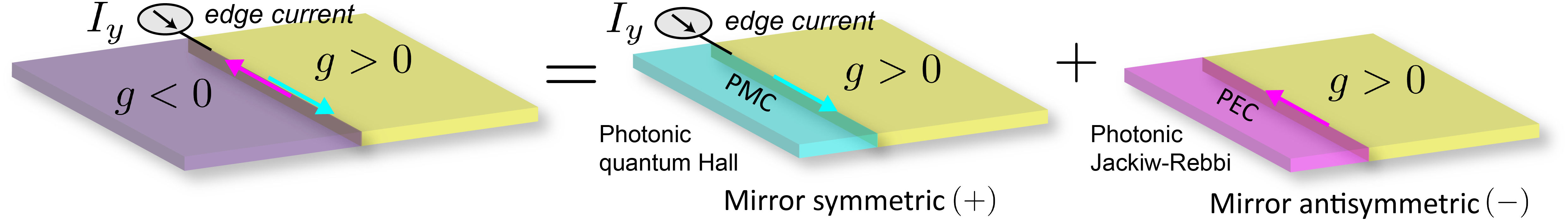
Figure 2: The interface of two optical isomers with positive $+g$ and negative $-g$ gyrotropy. In the Drude model, this corresponds to reversed magnetic biasing $\pm B_{0}$. The interface hosts two edge states that can be decomposed into two chiral (unidirectional) subsystems with perfect magnetic conductor (PMC) and perfect electric conductor (PEC) boundary conditions. PMC and PEC are mirror symmetric $(+)$ and mirror antiysmmetric $(-)$ respectively, designating photonic quantum Hall (PQH) and photonic Jackiw-Rebbi (PJR) states. The particular mirror symmetry $(\pm)$ dictates how the electromagnetic field transforms into the virtual photon $\mathcal{P}_{x}f(-x)=\pm f(x)$.

V Interface of optical isomers

In Sec. IV, we showed that nonlocal gyrotropy $g(\omega,k)$ can lead to topologically-protected chiral edge states that satisfy open boundary conditions. In the Drude model, this arises from a momentum dependent cyclotron frequency $\Omega_{c}(k)=\omega_{c}+\beta_{c}k^{2}$ that changes sign within the dispersion $\omega_{c}\beta_{c}<0$. Discovering such a material and observing these topological edge waves remains an open problem. Here, we consider a more practical scenario that does not involve nonlocality $\beta_{c}=0$, but hosts intriguing physics nonetheless.

Instead of having $g$ change sign with momentum, we let $g$ vary with position $g\to g(x)$ such that it defines the boundary between two distinct materials. The simplest case represents the boundary of two “optical isomers” Zhukov and Raikh (2000); Zyuzin and Zyuzin (2015), with $g$ in the $x>0$ space and $-g$ in the $x<0$ space but $\varepsilon$ identical in both media. The permittivity tensors are therefore complex conjugates of one another $\varepsilon_{ij}(x)=\varepsilon_{ij}^{*}(-x)$ and there is perfect mirror symmetry about $x=0$. In the Drude model, this represents the interface between two biased plasmas, but with reversed applied fields $\pm B_{0}$. The cyclotron frequencies in each half-space are exactly opposite $\pm\omega_{c}=\pm eB_{0}/M_{0}$. Note though, this implies the biasing field is discontinuous across the boundary $B_{0}(0^{+})\neq B_{0}(0^{-})$ which is an idealization. In reality, there must be a field gradient $B_{0}\to B_{0}(x)$ that interpolates between the two regions. However, we get this desired behavior for free if we assume a perfect mirror in the $x<0$ half-space, such that the virtual photon is the exact mirror image Horsley (2018). This is because the permittivity is even under mirror symmetry $\varepsilon\to\varepsilon$ while gyrotropy is odd $g\to-g$.

There are two types of mirrors we can introduce: a perfect magnetic conductor (PMC) or a perfect electric conductor (PEC). The difference between the two lies in the type of symmetry of the boundary condition. PMC represents symmetric $(+)$ boundary conditions and PEC is antisymmetric $(-)$. Under each symmetry ($\pm$) the electromagnetic field $f$ must transform into its mirror image as $\mathcal{P}_{x}f(-x)=\pm f(x)$. As we will see, each mirror has a chiral (unidirectional) edge state associated with it, but with very different properties. A visualization of the two mirror boundary conditions is displayed in Fig. 2. It must be stressed that a real interface of optical isomers hosts both edge states. A symmetric (PMC) state propagates in one direction while the antisymmetric (PEC) state propagates in the opposite direction. Only when we enforce a specific boundary condition can we isolate for either edge state.

VI Photonic quantum Hall (PQH) edge states

The photonic quantum Hall (PQH) edge states are symmetric (PMC) solutions of the optical isomer problem. These states are unique in that they support a high frequency quantum Hall edge current at the interface. The first step is to derive the $\delta$-potential characterizing the potential energy at the discontinuity $x=0$. This arises from a sudden change in the gyrotropic coefficient $g\to g~{}\mathrm{sgn}(x)$. Assuming the longitudinal field is nonzero $E_{y}\neq 0$, it can be shown that $E_{y}$ satisfies a Schrödinger-like wave equation,

$$-\partial_{x}^{2}E_{y}+V(x)E_{y}=\mathcal{E}E_{y}.$$ (42)

$V(x)$ is the “potential energy” and after differentiating reduces to a $\delta$-function,

$$V(x)=k_{y}\frac{g}{\varepsilon}\partial_{x}\mathrm{sgn}(x)=2k_{y}\frac{g}{\varepsilon}\delta(x).$$ (43)

$\mathcal{E}$ is the corresponding “energy eigenvalue”,

$$\mathcal{E}=\omega^{2}\left(\varepsilon-\frac{g^{2}}{\varepsilon}\right)-k_{y}^{2}.$$ (44)

It is well known that $\delta$-potentials always possess a bound state when the potential energy is attractive $V(x)<0$. Therefore, $k_{y}g/\varepsilon<0$ must always be satisfied for any given frequency and wave vector. The chirality of the bound state is immediately apparent. If a solution exists for a particular $k_{y}$, then $k_{y}\to-k_{y}$ is never a simultaneous solution. Back-scattering is forbidden.

To solve Eq. (42), we integrate both sides of the equation from $\int_{0^{-}}^{0^{+}}dx$ while assuming $E_{y}(x)=E_{y}(0)\exp(-\eta|x|)$. In this case, the longitudinal electric field is continuous across the domain wall $E_{y}(0^{+})=E_{y}(0^{-})$. We obtain a surprisingly simple characteristic equation,

$$\eta=-k_{y}\frac{g}{\varepsilon},\qquad k_{y}^{2}=\omega^{2}\varepsilon.$$ (45)

Notice that an edge state only exists when $\varepsilon>0$ is positive. This is very different from SPPs which require a negative permittivity. After some algebra, the $E_{x}$ and $H_{z}$ fields can be expressed as,

$$E_{x}(x)=-is_{x}\frac{\varepsilon^{2}+g^{2}}{2\varepsilon g}E_{y}(0)e^{-\eta|x|},$$ (46a)

$$H_{z}(x)=is_{x}s_{k_{y}}\frac{\varepsilon^{2}-g^{2}}{2\sqrt{\varepsilon}g}E_{y}(0)e^{-\eta|x|},$$ (46b)

where $s_{x}=\mathrm{sgn}(x)$ and $s_{k_{y}}=\mathrm{sgn}(k_{y})$ denotes the sign of $x$ and $k_{y}$ respectively. It is easy to check that the PQH state is mirror symmetric $\mathcal{P}_{x}f(-x)=+f(x)$ about $x=0$.

However, one might expect the normal electric field $E_{x}$ and tangential magnetic field $H_{z}$ to vanish at $x=0$ due to PMC boundary conditions. This is not the case. A free edge current is running parallel to the interface, such that the fields are discontinuous,

$$I_{y}=\frac{1}{2}\left[H_{z}(0^{-})-H_{z}(0^{+})\right]=-is_{k_{y}}\frac{\varepsilon^{2}-g^{2}}{2\sqrt{\varepsilon}g}E_{y}(0).$$ (47)

Note, we divide by a factor of 2 to remove the contribution from the virtual photon. $I_{y}$ is the high frequency analogue of the quantum Hall edge current. Interestingly, these photonic edge waves can be excited by passing a time-varying current along the boundary - similar to a transmission line Cheng (2013). However, current can only flow in one direction and the system behaves like a simultaneous photonic and electronic diode.

Now we look for self-consistent solutions to the dispersion relation [Eq. (45)] which correspond to propagating edge modes, with both $k_{y}$ and $\omega$ real-valued. There are in fact two edge bands which span the gaps between the bulk bands,

$$\omega^{2}_{\uparrow\downarrow}=\frac{1}{2}\left[\omega_{p}^{2}+\omega_{c}^{2}+k_{y}^{2}\pm\sqrt{(\omega_{p}^{2}+\omega_{c}^{2}+k_{y}^{2})^{2}-4k_{y}^{2}\omega_{c}^{2}}\right].$$ (48)

$\omega_{\uparrow}$ spans the region between the upper $\omega_{+}$ and lower $\omega_{-}$ bulk TM bands while $\omega_{\downarrow}$ spans between $\omega_{c}$ and $0$. Now we need to check when $\eta>0$ represents a decaying wave for the two edge modes,

$$\eta_{\uparrow\downarrow}=-k_{y}\frac{g(\omega_{\uparrow\downarrow})}{\varepsilon(\omega_{\uparrow\downarrow})}=\frac{k_{y}\omega_{c}\omega_{p}^{2}}{\omega_{\uparrow\downarrow}(\omega_{\uparrow\downarrow}^{2}-\omega_{p}^{2}-\omega_{c}^{2})}.$$ (49)

Since $\omega_{\uparrow}^{2}\geq\omega_{p}^{2}+\omega_{c}^{2}$ for all $k_{y}$, then $\omega_{c}k_{y}>0$ must always be satisfied in the $\omega_{\uparrow}$ frequency region. Choosing $\omega_{c}>0$, the upper edge branch propagates strictly in the $k_{y}>0$ direction. Similarly, since $\omega_{\downarrow}^{2}<\omega_{p}^{2}+\omega_{c}^{2}$ for all $k_{y}$, then $\omega_{c}k_{y}<0$ must always be satisfied in the $\omega_{\downarrow}$ frequency region. The lower edge branch propagates strictly in the $k_{y}<0$ direction. The dispersion relation of the PQH edge states are displayed in Fig. 3.

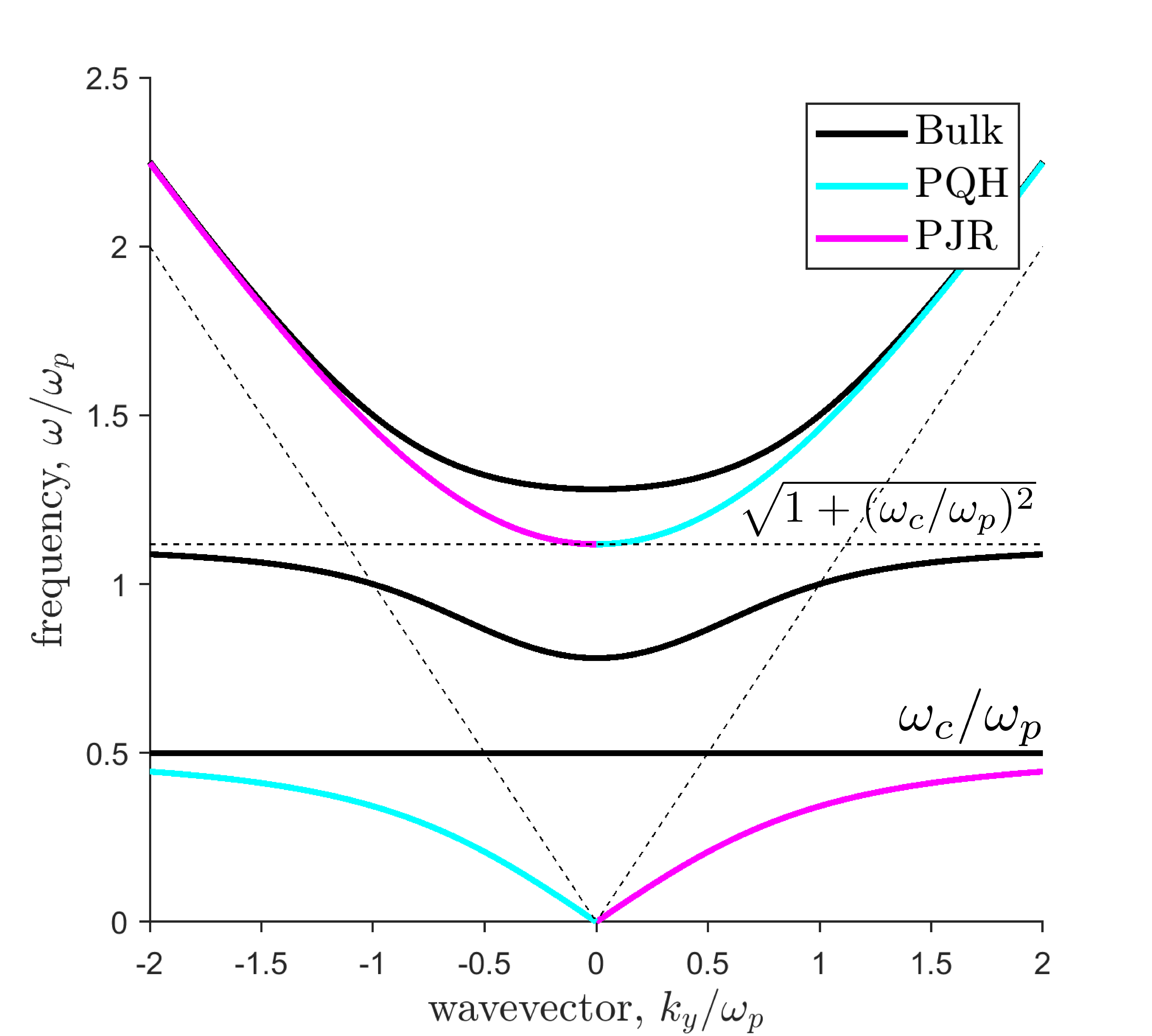
Figure 3: Dispersion relation of the local Drude model under an applied magnetic field with $\omega_{c}/\omega_{p}=1/2$ as an example. Black lines indicate bulk bands while cyan and magnetic lines represent unidirectional photonic quantum Hall (PQH) and photonic Jackiw-Rebbi (PJR) edge states respectively. There are a total of 3 positive energy bulk bands. Two correspond to high and low frequency TM modes $\omega=\omega_{\pm}$ while the third represents pure cyclotron orbits $\omega=\omega_{c}$. The PQH states emerge at a PMC boundary while the PJR states require a PEC boundary. Unlike conventional SPPs, the PQH and PJR states asymptotically approach the bulk bands in the $k_{y}\to\infty$ limit. The upper branch approaches the free photon dispersion $\omega_{\uparrow}\to k_{y}$ while the lower branch approaches pure cyclotron orbits $\omega_{\downarrow}\to\omega_{c}$. The frequency range where no edge state exists $\omega_{c}<\omega<\sqrt{\omega_{p}^{2}+\omega_{c}^{2}}$, corresponds to the plasmonic region $\varepsilon<0$. Indeed, these edge waves are fundamentally different from SPPs as they require $\varepsilon>0$.

VII Photonic Jackiw-Rebbi (PJR) edge states

The photonic Jackiw-Rebbi (PJR) edge states are antisymmetric (PEC) solutions of the optical isomer problem. Like the QGEE, these edge states are completely transverse electro-magnetic (TEM) waves. PJR states share many important properties with the QGEE [Sec. IV] even though they arise by a very different means. The only significant difference is that they do not satisfy open boundary conditions and necessarily require a PEC boundary. This means they are not topologically-protected as they are sensitive to boundary conditions. However, this particular system is the most practical experimentally.

To solve, we first assume the magnetic field is continuous across the domain wall $H_{z}(0^{+})=H_{z}(0^{-})$ such that zero edge current $I_{y}=0$ is excited. We obtain an identical dispersion relation as the PQH states [Eq. (45)], except the wave propagates in the reverse direction,

$$\eta=k_{y}\frac{g}{\varepsilon},\qquad k_{y}^{2}=\omega^{2}\varepsilon.$$ (50)

There is an immediate connection with the Dirac Jackiw-Rebbi dispersion [Eq. (56)], with respect to the effective speed of light $v_{p}$ and effective photon mass $\Lambda_{p}$,

$$\eta=\frac{\omega g}{\sqrt{\varepsilon}}=\frac{|\Lambda_{p}|}{v_{p}},\qquad\omega^{2}=\frac{k_{y}^{2}}{\varepsilon}=v_{p}^{2}k_{y}^{2}.$$ (51)

Surprisingly, the electromagnetic field profile of the PJR state is drastically different than the PQH state. The longitudinal field vanishes $E_{y}(x)=0$ entirely because $E_{y}(0^{+})=E_{y}(0^{-})=0$ is required by symmetry. Hence, the PEC states correspond to completely transverse electro-magnetic (TEM) edge waves,

$$f(x)=E_{x}(0)\Big{(}\hat{x}-s_{k_{y}}\sqrt{\varepsilon}\hat{z}\Big{)}e^{-\eta|x|}.$$ (52)

It is easy to check that the PJR state is mirror antisymmetric $\mathcal{P}_{x}f(-x)=-f(x)$ about $x=0$. The edge wave behaves identically to a vacuum photon (transverse polarized) but with a modified dispersion. Indeed, they are helically quantized along the direction of propagation $\hat{k}\cdot\vec{E}=\hat{y}\cdot\vec{E}=E_{y}=0$. This is the definition of longitudinal spin-momentum locking as $f$ is an eigenstate of $\hat{S}_{y}$,

$$\hat{S}_{y}\mathfrak{F}=s_{k_{y}}\mathfrak{F},\qquad\mathfrak{F}=\begin{bmatrix}\sqrt{\varepsilon}E_{x}\\ \sqrt{\varepsilon}E_{y}\\ H_{z}\end{bmatrix}.$$ (53)

$\hat{k}\cdot\vec{S}=\hat{S}_{y}$ is the helicity operator along $\hat{y}$, which was defined in Eq. (3). Notice that the spin is quantized $s_{k_{y}}=\mathrm{sgn}(k_{y})=\pm 1$ and completely locked to the momentum as it depends on the direction of propagation. This should be contrasted with their electron (spin-$\nicefrac{{1}}{{2}}$) equivalent in Eq. (57). The dispersion relation of the PJR edge states are displayed in Fig. 3. A short discussion on the robustness of PQH and PJR states is presented in Appendix B.

VIII Conclusion

In summary, we have identified the three fundamental classes of unidirectional photonic edge waves arising in gyroelectric media. The quantum gyroelectric effect (QGEE) is a topologically-protected edge state that requires nonlocal gyrotropy. This wave satisfies open boundary conditions and displays bulk-boundary correspondence as it is defined independent of the contacting medium. The photonic quantum Hall (PQH) and photonic Jackiw-Rebbi (PJR) states are local phenomena and emerge at the interface of optical isomers - two media with inverted gyrotropy.

Appendix

Appendix A Dirac Jackiw-Rebbi edge states

For completeness, we provide a brief review of Jackiw-Rebbi states that arise in two-dimensional condensed matter systems. The simplest realization is described by the 2D Dirac equation $H\Psi=E\Psi$,

$$H=v(k_{x}\sigma_{x}+k_{y}\sigma_{y})+\Lambda\sigma_{z},$$ (54)

where $[\sigma_{i},\sigma_{j}]=2i\epsilon_{ijk}\sigma_{k}$ are the Pauli matrices. $v$ is the Fermi velocity and $\Lambda$ is a two-dimensional Dirac mass.

We consider an interface of two Dirac particles with opposite masses $\Lambda\to\Lambda\mathrm{sgn}(x)$. Similar to the photonic problem [Sec. V], there is now mirror symmetry about $x=0$. The unidirectional (chiral) edge solution is well known Shen et al. (2011) and assumes a surprisingly simple form,

$$\Psi(x)=\Psi_{0}\begin{bmatrix}1\\ i~{}s_{k_{y}}\end{bmatrix}e^{-\eta|x|},$$ (55)

where $s_{k_{y}}=\mathrm{sgn}(k_{y})=\pm 1$ is the sign of the momentum. This follows from the characteristic equation,

$$\eta=\frac{|\Lambda|}{v},\qquad E^{2}=v^{2}k_{y}^{2}.$$ (56)

If $\Lambda>0$, the Dirac edge wave propagates strictly in the $k_{y}>0$ direction and vice verse for $\Lambda<0$. It is clear that $\Psi$ is an eigenstate of both the helicity operator $\hat{k}\cdot\vec{S}=\sigma_{y}/2$ and the mirror operator $\mathcal{P}_{x}=\sigma_{y}$ which are identical in this case,

$$\sigma_{y}\Psi(-x)=\sigma_{y}\Psi(x)=s_{k_{y}}\Psi(x).$$ (57)

Indeed, the Dirac Jackiw-Rebbi edge states are helically quantized and behave identically to a massless (Weyl) fermion. This should be contrasted with their photonic (spin-1) equivalent in Eq. (53).

Appendix B Robustness of PQH and PJR edge states

Although the PQH and PJR states are not topologically-protected, they can still exhibit robust transport - ie. immunity to small perturbations in the gyrotropic coefficient $g$. Let us assume $g\to g(x)$ is a function of $x$ but take $\varepsilon$ as a constant in space. In reality, this is only approximately true since $g$ and $\varepsilon$ cannot be completely independent functions. In the Drude model for instance, a field gradient $B_{0}\to B_{0}(x)$ creates a spatially dependent cyclotron frequency $\omega_{c}\to\omega_{c}(x)$ which alters both the resonance frequency and the relative magnitude of the gyrotropy. Hence, both $g$ and $\varepsilon$ will generally vary with $x$. However, this simplifying assumption illustrates the point very well and holds for relatively small perturbations in the gyrotropy.

When only $g(x)$ varies with $x$, the Schrödinger-like wave equation [Eq. (42)] for the PQH state becomes,

$$-\partial_{x}^{2}E_{y}+\left[\frac{k_{y}}{\varepsilon}\partial_{x}g(x)+\omega^{2}\frac{g^{2}(x)}{\varepsilon}\right]E_{y}=(\omega^{2}\varepsilon-k_{y}^{2})E_{y}.$$ (58)

Due to the mirror boundary condition, $g(-x)=-g(x)$ is an odd function of $x$. However, we can still allow a jump discontinuity at $x=0$, such that $g(0^{-})=-g(0^{+})$. Far from the boundary $|x|\to\infty$, the gyrotropy approaches the uniform bulk $g(x\to\pm\infty)=\pm g_{0}$. A unidirectional edge state always exists and is immune to perturbations in $g$. To prove this, we choose an integrating factor of the form,

$$E_{y}(x)=E_{y}(0)\exp\left[\frac{k_{y}}{\varepsilon}\int_{-\infty}^{x}g(x^{\prime})dx^{\prime}\right],$$ (59)

which satisfies,

$$\partial_{x}E_{y}(x)=\frac{k_{y}}{\varepsilon}g(x)E_{y}(x),$$ (60)

and,

$$\partial_{x}^{2}E_{y}(x)=\left[\frac{k_{y}}{\varepsilon}\partial_{x}g(x)+\frac{k_{y}^{2}}{\varepsilon^{2}}g^{2}(x)\right]E_{y}(x).$$ (61)

Clearly, if the edge dispersion is fulfilled $k_{y}^{2}=\omega^{2}\varepsilon$, Eq. (58) is satisfied regardless of the particular form of $g(x)$. The exact same integrating solution exists for the PJR states, with $E_{y}(x)=0$, except the momentum is reversed $k_{y}\to-k_{y}$.

As an example, let $g(x)=g_{0}\tanh(x/a)$, where $a$ is some characteristic transition length that interpolates between $g(0)=0$ and $g(x\to\pm\infty)=\pm g_{0}$. The integral of which is $\int g(x^{\prime})dx^{\prime}=ag_{0}\log[\cosh(x/a)]$. The spatial profile then becomes,

$$E_{y}(x)=E_{y}(0)[\cosh(x/a)]^{(k_{y}ag_{0}/\varepsilon)}.$$ (62)

In the limit of an infinitesimally narrow transition width $a\to 0$, the solution reduces to the idealized case $[\cosh(x/a)]^{(k_{y}ag_{0}/\varepsilon)}\to\exp(-\eta|x|)$ with $\eta=-k_{y}g_{0}/\varepsilon$.

Appendix C Temporal dispersion

Temporal dispersion, or the frequency dependence of linear response, arises whenever light couples to matter,

$$\mathcal{M}(\omega)=\begin{bmatrix}\varepsilon_{xx}&\varepsilon_{xy}&\chi_{x}\\ \varepsilon_{xy}^{*}&\varepsilon_{yy}&\chi_{y}\\ \chi_{x}^{*}&\chi_{y}^{*}&\mu\end{bmatrix},~{}~{}\begin{array}[]{ll}D_{i}=\varepsilon_{ij}E^{j}+\chi_{i}H_{z},\\ {}\\ B_{z}=\chi_{i}^{*}E^{i}+\mu H_{z}.\\ \end{array}$$ (63)

Temporal dispersion is always present because it characterizes the relative coupling at a particular energy to the material degrees of freedom - the electronic modes. These are the physical objects that generate the linear response theory to begin with. Moreover, due to the reality condition of the electromagnetic field (particle-antiparticle symmetry), the real and imaginary components of $\mathcal{M}$ cannot be arbitrary functions of $\omega$,

$$\mathcal{M}^{*}(-\omega)=\mathcal{M}(\omega).$$ (64)

This implies $\Re[\mathcal{M}(-\omega)]=\Re[\mathcal{M}(\omega)]$ must be even in $\omega$ while $\Im[\mathcal{M}(-\omega)]=-\Im[\mathcal{M}(\omega)]$ is odd. Hence, it is physically impossible to break time-reversal ($\mathcal{T}$) symmetry without dispersion not . In this case, we imply breaking $\mathcal{T}$ symmetry nontrivially (Hermitian response). Adding loss (antiHermitian response) breaks $\mathcal{T}$ symmetry in a trivial way because it does not alter the dynamics of the field - it simply adds a finite lifetime.

Besides the reality condition, $\mathcal{M}$ must satisfy three additional physical constraints. The first being transparency at high frequency,

$$\lim_{\omega\to\infty}\mathcal{M}(\omega)\to\mathds{1}_{3},$$ (65)

where $\mathds{1}_{3}$ is the $3\times 3$ identity. The second being Kramers-Kronig (causality),

$$\oint_{\Im[\omega^{\prime}]\geq 0}\frac{\mathcal{M}(\omega^{\prime})-\mathds{1}_{3}}{\omega^{\prime}-\omega}d\omega^{\prime}=0.$$ (66)

This ensures the response function is analytic in the upper complex plane and decays at least as fast as $|\omega|^{-1}$. The last condition requires a positive definite energy density,

$$\bar{\mathcal{M}}(\omega)=\partial_{\omega}[\omega\mathcal{M}(\omega)]>0.$$ (67)

By combining all the aforementioned constraints and assuming Hermitian (lossless) systems $\mathcal{M}^{\dagger}=\mathcal{M}$, we can always expand $\mathcal{M}$ via a partial fraction decomposition,

$$\mathcal{M}(\omega)=\mathds{1}_{3}-\sum_{\alpha}\frac{\mathcal{C}_{\alpha}^{\dagger}\mathcal{C}_{\alpha}}{\omega_{\alpha}(\omega-\omega_{\alpha})}.$$ (68)

The poles of the response function $\omega=\omega_{\alpha}$ represent resonances of the material degrees of freedom. From an electronic band structure point of view, $\omega_{\alpha}=(E_{\alpha}-E_{0})/\hbar$ represents the energy difference between the ground state and an excited state. $\mathcal{C}_{\alpha}$ is the coupling strength (matrix element) of the excitation.

Appendix D Spatial dispersion (nonlocality)

Spatial dispersion, or the momentum dependence of linear response, dictates how the light-matter interaction changes with wavelength (scale). Nonlocality becomes relevant at the nanoscale and governs the deep subwavelength physics. Perhaps more importantly, nonlocality is fundamentally necessary to describe topological phenomena. As has been proven in Ref. Van Mechelen and Jacob (2018b); Mechelen and Jacob (2019), Chern numbers are only quantized when $\mathcal{M}$ is regularized which inherently requires spatial dispersion. This is the only way for the electromagnetic theory to be consistent with the tenfold way Ryu et al. (2010), which describes all possible continuum topological theories. Technically, the photon belongs to Class D, the same universality class as the $p+ip$-wave topological superconductor Read and Green (2000). Class D possesses an integer topological invariant (Chern number) in two dimensions.

Spatial dispersion is easily introduced by letting $\omega_{\alpha}\to\omega_{\alpha\mathbf{k}}$ and $\mathcal{C}_{\alpha}\to\mathcal{C}_{\alpha\mathbf{k}}$ be functions of $\mathbf{k}$,

$$\mathcal{M}(\omega,\mathbf{k})=\mathds{1}_{3}-\sum_{\alpha}\frac{\mathcal{C}_{\alpha\mathbf{k}}^{\dagger}\mathcal{C}_{\alpha\mathbf{k}}}{\omega_{\alpha\mathbf{k}}(\omega-\omega_{\alpha\mathbf{k}})}.$$ (69)

The $\mathbf{k}$ dependence cannot be completely arbitrary because the response function must satisfy the generalized reality condition,

$$\mathcal{M}^{*}(-\omega,-\mathbf{k})=\mathcal{M}(\omega,\mathbf{k}).$$ (70)

The reality condition (particle-antiparticle symmetry) implies there is a negative energy resonance $-\omega_{\alpha-\mathbf{k}}$ associated with each positive energy $\omega_{\alpha\mathbf{k}}$. The wave equation of the 2D photon coupled to matter is thus,

$$\mathcal{H}_{0}(\mathbf{k})f=\omega\mathcal{M}(\omega,\mathbf{k})f.$$ (71)

However, this is still not a first-order eigenvalue problem since $\mathcal{M}$ depends on the eigenvalue $\omega$ itself. Moreover, the electromagnetic field $f$ is not the complete eigenvector of this system. A simple reason is because the number of eigenmodes $n$ should match the dimensionality of the eigenvector $\dim[u]=n$. This clearly does not hold $\dim[f]=3$ when temporal dispersion is present since there can be many modes that satisfy the wave equation [Eq. (71)].

D.1 Electromagnetic Hamiltonian

To convert Eq. (71) into a first-order Hamiltonian, we define the auxiliary variables $\psi_{\alpha}$ that describe the internal polarization and magnetization modes of the medium,

$$\psi_{\alpha}=\frac{\mathcal{C}_{\alpha\mathbf{k}}f}{\omega-\omega_{\alpha\mathbf{k}}},\qquad\omega\psi_{\alpha}=\omega_{\alpha\mathbf{k}}\psi_{\alpha}+\mathcal{C}_{\alpha\mathbf{k}}f.$$ (72)

Back-substituting into Eq. (71) and using the partial fraction expansion,

$$\frac{\omega}{\omega_{\alpha}(\omega-\omega_{\alpha})}=\frac{1}{\omega_{\alpha}}+\frac{1}{\omega-\omega_{\alpha}},$$ (73)

we obtain the first-order wave equation,

$$H(\mathbf{k})u=\omega u,\qquad u=\begin{bmatrix}f\\ \psi_{1}\\ \psi_{2}\\ \vdots\end{bmatrix}.$$ (74)

$u$ accounts for the electromagnetic field $f$ and all internal polarization modes $\psi_{\alpha}$ describing the linear response. $H(\mathbf{k})$ is the Hamiltonian matrix that acts on this generalized state vector $u$,

$$H(\mathbf{k})=\begin{bmatrix}\mathcal{H}_{0}(\mathbf{k})+\sum_{\alpha}\omega_{\alpha\mathbf{k}}^{-1}\mathcal{C}^{\dagger}_{\alpha\mathbf{k}}\mathcal{C}_{\alpha\mathbf{k}}&~{}~{}\mathcal{C}^{\dagger}_{1\mathbf{k}}~{}~{}&~{}~{}\mathcal{C}^{\dagger}_{2\mathbf{k}}~{}~{}&\ldots\\ \mathcal{C}_{1\mathbf{k}}&\omega_{1\mathbf{k}}&0&\ldots\\ \mathcal{C}_{2\mathbf{k}}&0&\omega_{2\mathbf{k}}&\ldots\\ \vdots&\vdots&\vdots&\ddots\end{bmatrix}.$$ (75)

This decomposition makes intuitive sense. The dimensionality of the Hamiltonian matches the number of distinct eigenmodes and eigenenergies of the problem. The complete set of eigenvectors is thus,

$$H(\mathbf{k})u_{n\mathbf{k}}=\omega_{n\mathbf{k}}u_{n\mathbf{k}}.$$ (76)

Constructing the total Hamiltonian $H(\mathbf{k})$ is a very important procedure when nonlocality is present. This is because we have to start imposing boundary conditions on the oscillators $\psi_{\alpha}$ themselves when we consider interface effects.

Utilizing the linear response theory, the electromagnetic eigenstates of the medium $f_{n\mathbf{k}}$ are solutions of the self-consistent wave equation,

$$\det[\omega\mathcal{M}(\omega,\mathbf{k})-\mathcal{H}_{0}(\mathbf{k})]=0,\qquad\omega=\omega_{n\mathbf{k}},$$ (77)

which determines all possible polaritonic bands. These bands are normalized to the energy density as,

$$u^{\dagger}_{n\mathbf{k}}u_{n\mathbf{k}}=f^{\dagger}_{n\mathbf{k}}\bar{\mathcal{M}}(\omega_{n\mathbf{k}},\mathbf{k})f_{n\mathbf{k}}=1,$$ (78)

where,

$$\bar{\mathcal{M}}(\omega,\mathbf{k})=\partial_{\omega}[\omega\mathcal{M}(\omega,\mathbf{k})]=\mathds{1}_{3}+\sum_{\alpha}\frac{\mathcal{C}^{\dagger}_{\alpha\mathbf{k}}\mathcal{C}_{\alpha\mathbf{k}}}{(\omega-\omega_{\alpha\mathbf{k}})^{2}}.$$ (79)

Due to the constraints on $\mathcal{M}$, these bands are continuous and real-valued for all $\mathbf{k}$.

D.2 Nonlocal regularization

A well known requirement of any continuum topological theory, is that the Hamiltonian must approach a directionally independent value in the asymptotic limit Ryu et al. (2010),

$$\lim_{k\to\infty}H(\mathbf{k})=H(k).$$ (80)

This ensures the Hamiltonian is connected at infinity and is the continuum equivalent of a periodic boundary condition. Mathematically, this means the momentum space manifold is compact and can be projected onto the Riemann sphere $\mathbb{R}^{2}\to S^{2}$. Alternatively, if the response function is regularized, the wave equation approaches a directionally independent value in the asymptotic limit,

$$\lim_{k\to\infty}[\omega\mathcal{M}(\omega,\mathbf{k})-\mathcal{H}_{0}(\mathbf{k})]\to\omega\mathcal{M}(\omega,k).$$ (81)

This places constraints on the asymptotic behavior of the response parameters,

$$\lim_{k\to\infty}\mathcal{C}_{\alpha\mathbf{k}}\to\mathcal{C}_{\alpha p}k^{p},\qquad\lim_{k\to\infty}\omega_{\alpha\mathbf{k}}\to\omega_{\alpha p}k^{p}.$$ (82)

Consequently, $\mathcal{C}_{\alpha\mathbf{k}}$ and $\omega_{\alpha\mathbf{k}}$ require quadratic order nonlocality at minimum $p\geq 2$ to be properly regularized. We will show that this is a necessary and sufficient condition for Chern number quantization.

Appendix E Continuum electromagnetic Chern number

The Berry connection is found by varying the complete eigenvectors $u_{n\mathbf{k}}$ with respect to the momentum $\mathbf{A}_{n}(\mathbf{k})=-iu^{\dagger}_{n\mathbf{k}}\partial_{\mathbf{k}}u_{n\mathbf{k}}$. This can be simplified to,

$$\mathbf{A}_{n}(\mathbf{k})=-if^{\dagger}_{n\mathbf{k}}\bar{\mathcal{M}}(\omega_{n\mathbf{k}},\mathbf{k})\partial_{\mathbf{k}}f_{n\mathbf{k}}+f^{\dagger}_{n\mathbf{k}}\boldsymbol{\mathcal{A}}(\omega_{n\mathbf{k}},\mathbf{k})f_{n\mathbf{k}},$$ (83)

where $\boldsymbol{\mathcal{A}}$ is the Berry connection arising from the material degrees of freedom,

$$\boldsymbol{\mathcal{A}}(\omega,\mathbf{k})=-i\sum_{\alpha}\frac{\mathcal{C}^{\dagger}_{\alpha\mathbf{k}}\partial_{\mathbf{k}}\mathcal{C}_{\alpha\mathbf{k}}}{(\omega-\omega_{\alpha\mathbf{k}})^{2}}.$$ (84)

It is straightforward to prove that nonlocal regularization guarantees Chern number quantization. In the asymptotic limit, the electromagnetic modes approach a directionally independent value, up to a possible U(1) gauge,

$$\lim_{k\to\infty}f_{n}(\mathbf{k})\to f_{n}(k)\exp\left[i\chi_{n}(\mathbf{k})\right].$$ (85)

The closed loop at $k=\infty$ is therefore a pure gauge, which is necessarily a unit Berry phase,

$$\begin{split}\exp\left[i\oint_{k=\infty}\mathbf{A}_{n}(\mathbf{k})\cdot d\mathbf{k}\right]&=\exp\left[i\chi_{n}|_{0}^{2\pi}\right]=1\\ &=\exp\left[i\int_{\mathbb{R}^{2}}F_{n}(\mathbf{k})d^{2}\mathbf{k}\right].\end{split}$$ (86)

$F_{n}(\mathbf{k})=\hat{z}\cdot[\partial_{\mathbf{k}}\times\mathbf{A}_{n}(\mathbf{k})]$ is the Berry curvature and we have utilized Stokes’ theorem to convert the line integral to a surface integral over the entire planar momentum space $\mathbb{R}^{2}$. Since the total Berry flux must come in multiples of $2\pi$, the Chern number $C_{n}$ is guaranteed to be an integer,

$$C_{n}=\frac{1}{2\pi}\int_{\mathbb{R}^{2}}F_{n}(\mathbf{k})d^{2}\mathbf{k}\in\mathbb{Z}.$$ (87)

$C_{n}$ counts the number of singularities in the gauge potential $\mathbf{A}_{n}(\mathbf{k})$ as it evolves over the momentum space. We will now discuss the role of symmetries on the electromagnetic Chern number - specifically rotational symmetry.

Appendix F Rotational symmetry and spin

If the unit cell of the atomic crystal possesses a center (at least threefold cyclic) the response function is rotationally symmetric about $z$,

$$\mathcal{R}^{-1}\mathcal{M}(\omega,R\mathbf{k})\mathcal{R}=\mathcal{M}(\omega,\mathbf{k}).$$ (88)

$R$ is the SO(2) matrix acting on the coordinates $\mathbf{k}$. $\mathcal{R}$ is the action of SO(2) acting on the fields $f$, which induces rotations in the $x$-$y$ plane,

$$R=\begin{bmatrix}\cos\theta&\sin\theta\\ -\sin\theta&\cos\theta\end{bmatrix},~{}~{}~{}~{}\mathcal{R}=\exp(i\theta\hat{S}_{z})=\begin{bmatrix}R&0\\ 0&1\end{bmatrix}.$$ (89)

$\mathcal{R}$ is simply the SO(3) matrix along $\hat{z}$ which rotates the polarization state of the electromagnetic field. Clearly the representation is single-valued (bosonic) and describes a spin-1 particle,

$$\mathcal{R}(2\pi)=\mathds{1}_{3}.$$ (90)

Infinitesimal rotations on the coordinates $\mathbf{k}$ gives rise to the orbital angular momentum (OAM) $\hat{L}_{z}=-i\partial_{\phi}$ while infinitesimal rotations on the polarization state gives rise to the spin angular momentum (SAM) $\hat{S}_{z}=-i\epsilon_{ijz}$. Consequently, the total angular momentum (TAM) $\hat{J}_{z}$ is conserved, at all frequencies and wave vectors,

$$[\hat{J}_{z},\mathcal{M}(\omega,\mathbf{k})]=0,\qquad\hat{J}_{z}=\hat{L}_{z}+\hat{S}_{z}.$$ (91)

This implies the electromagnetic field is a simultaneous eigenstate of $\hat{J}_{z}$,

$$\hat{J}_{z}f_{n\mathbf{k}}=j_{n}f_{n\mathbf{k}},\qquad j_{n}\in\mathbb{Z}.$$ (92)

$j_{n}$ is necessarily an integer for photons. Note though, $j_{n}$ is only uniquely defined up to a gauge since we can always add an arbitrary OAM to the state $f_{n\mathbf{k}}\to f_{n\mathbf{k}}\exp(il_{n}^{\prime}\phi)$ such that $j_{n}\to j_{n}+l_{n}^{\prime}$.

F.1 Stationary (high-symmetry) points

At an arbitrary momentum $\mathbf{k}$, the SAM and OAM are not good quantum numbers - only the TAM is well defined (up to a gauge). However, at stationary points $k=k_{i}$, also known as high-symmetry points (HSPs), the electromagnetic field is a simultaneous eigenstate of $\hat{S}_{z}$ and $\hat{L}_{z}$. In the continuum limit there are two such HSPs, $k_{i}=0$ and $k_{i}=\infty$. At these specific momenta, the response function is rotationally invariant - it commutes with $\mathcal{R}$,

$$[\mathcal{R},\mathcal{M}(\omega,k_{i})]=[\hat{S}_{z},\mathcal{M}(\omega,k_{i})]=[\hat{L}_{z},\mathcal{M}(\omega,k_{i})]=0.$$ (93)

Since $\mathcal{M}$ is a continuous function of $\mathbf{k}$, it cannot depend on the azimuthal coordinate $\phi$ at HSPs, otherwise $\mathcal{M}$ would be multivalued. Hence, the electromagnetic field is an eigenstate of both $\hat{S}_{z}$ and $\hat{L}_{z}$ at $k_{i}$,

$$\hat{S}_{z}f_{n\mathbf{k}_{i}}=m_{n}(k_{i})f_{n\mathbf{k}_{i}},\qquad\hat{L}_{z}f_{n\mathbf{k}_{i}}=l_{n}(k_{i})f_{n\mathbf{k}_{i}}.$$ (94)

$m_{n}(k_{i})=\pm 1,0$ is the SAM eigenvalue at $k_{i}$ of the $n$th band and $l_{n}(k_{i})\in\mathbb{Z}$ is the OAM eigenvalue. Importantly, only the SAM is gauge invariant because it represents the eigenvalue of a matrix - ie. it only depends on the polarization state. This immediately implies the eigenmode can be factored into a spin and orbital part at HSPs,

$$f_{n\mathbf{k}_{i}}\propto[e_{m}(k_{i})]_{n}\exp[il_{n}(k_{i})\phi].$$ (95)

$[e_{m}(k_{i})]_{n}$ is the particular spin eigenstate at $k_{i}$ for the $n$th band. There are three possible eigenstates $e_{m}$ corresponding to three quantized spin-1 vectors,

$$\mathcal{R}e_{m}=e^{im\theta}e_{m},\qquad\hat{S}_{z}e_{m}=me_{m},$$ (96)

where $m=\pm 1,0$ labels the quantum of spin for each state,

$$e_{\pm}=\frac{1}{\sqrt{2}}\begin{bmatrix}1\\ \pm i\\ 0\end{bmatrix},\qquad e_{0}=\begin{bmatrix}0\\ 0\\ 1\end{bmatrix}.$$ (97)

$e_{\pm}$ are right and left-handed states respectively and represent electric resonances $E_{y}=\pm iE_{x}$ with $H_{z}=0$. The spin-0 state $e_{0}$ is a magnetic resonance $E_{x}=E_{y}=0$ with $H_{z}\neq 0$.

F.2 Spin spectrum

To determine the spin state of a particular band $n$, we need to solve the wave equation at HSPs. At these points, only three parameters are permitted by symmetry,

$$\mathcal{M}(\omega,k_{i})=\begin{bmatrix}\varepsilon&ig&0\\ -ig&\varepsilon&0\\ 0&0&\mu\end{bmatrix}.$$ (98)

$\varepsilon$ and $\mu$ are the scalar permittivity and permeability respectively. $g$ is the gyrotropic coefficient which breaks both time-reversal ($\mathcal{T}$) and parity ($\mathcal{P}$) symmetry but preserves rotational ($\mathcal{R}$) symmetry. Assuming a regularized response function, nontrivial solutions of the wave equation simultaneously satisfy,

$$\det[\mathcal{M}(\omega,k_{i})]=0,\qquad\omega=\omega_{n}(k_{i})\neq 0.$$ (99)

There are three possible conditions that satisfy Eq. (99). The first two generate right or left-handed states $e_{\pm}$,

$$m_{n}(k_{i})=\frac{g(\omega_{n}(k_{i}),k_{i})}{\varepsilon(\omega_{n}(k_{i}),k_{i})}=\pm 1.$$ (100)

The last generates the the spin-0 state $e_{0}$,

$$m_{n}(k_{i})=\mu(\omega_{n}(k_{i}),k_{i})=0.$$ (101)

Note, since $m_{n}$ is a discrete quantum number, it cannot vary continuously if rotational symmetry is preserved. It can only be changed at a topological phase transition which requires an accidental degeneracy at a HSP.

F.3 Symmetry-protected topological (SPT) phases

Remarkably, the electromagnetic Chern number is determined entirely from the spin eigenvalues at the HSPs $k_{i}$. The proof is surprisingly simple. Due to rotational symmetry, the Berry curvature $F_{n}(k)=\partial_{k}A_{n}^{\phi}(k)$ depends only on the magnitude of $k$ since $F_{n}$ is a scalar. Integrating the Berry curvature over all space $\mathbb{R}^{2}$, we arrive at,

$$C_{n}=A_{n}^{\phi}(\infty)-A_{n}^{\phi}(0)=l_{n}(\infty)-l_{n}(0).$$ (102)

This follows because $f_{n\mathbf{k}_{i}}$ is an eigenstate of the OAM at HSPs $k_{i}=0$ and $k_{i}=\infty$. The OAM at $k_{i}$ is not gauge invariant, however the difference at the two stationary points is gauge invariant because the TAM is conserved $j_{n}=m_{n}(0)+l_{n}(0)=m_{n}(\infty)+l_{n}(\infty)$. Substituting for $m_{n}$ we obtain,

$$C_{n}=m_{n}(0)-m_{n}(\infty).$$ (103)

Hence, the spin eigenstate must change at HSPs $m_{n}(0)\neq m_{n}(\infty)$ to acquire a nontrivial phase $C_{n}\neq 0$. It is also clear that a purely gyrotropic medium $\mu=1$ always has Chern numbers of $|C_{n}|=2$ since $m_{n}(k_{i})=\pm 1$ only assumes two values. $|C_{n}|=1$ is much more exotic as it requires both gyrotropy and magnetism.

References

- Mackay and Lakhtakia (2016) Tom G. Mackay and Akhlesh Lakhtakia, “Nonreciprocal dyakonov-wave propagation supported by topological insulators,” J. Opt. Soc. Am. B 33, 1266–1270 (2016).
- Caloz et al. (2018) Christophe Caloz, Andrea Alù, Sergei Tretyakov, Dimitrios Sounas, Karim Achouri, and Zoé-Lise Deck-Léger, “Electromagnetic nonreciprocity,” Phys. Rev. Applied 10, 047001 (2018).
- Mirmoosa et al. (2014) M. S. Mirmoosa, Y. Ra’di, V. S. Asadchy, C. R. Simovski, and S. A. Tretyakov, “Polarizabilities of nonreciprocal bianisotropic particles,” Phys. Rev. Applied 1, 034005 (2014).
- Valente et al. (2015) João Valente, Jun-Yu Ou, Eric Plum, Ian J. Youngs, and Nikolay I. Zheludev, “A magneto-electro-optical effect in a plasmonic nanowire material,” Nature Communications 6, 7021 EP – (2015), article.
- Floess and Giessen (2018) Dominik Floess and Harald Giessen, “Nonreciprocal hybrid magnetoplasmonics,” Reports on Progress in Physics 81, 116401 (2018).
- Zyuzin (2017) Vladimir A. Zyuzin, “Landau levels for an electromagnetic wave,” Phys. Rev. A 96, 043830 (2017).
- Mann et al. (2019) Sander A. Mann, Dimitrios L. Sounas, and Andrea Alù, “Nonreciprocal cavities and the time–bandwidth limit,” Optica 6, 104–110 (2019).
- Tsakmakidis et al. (2017) K. L. Tsakmakidis, L. Shen, S. A. Schulz, X. Zheng, J. Upham, X. Deng, H. Altug, A. F. Vakakis, and R. W. Boyd, “Breaking lorentz reciprocity to overcome the time-bandwidth limit in physics and engineering,” Science 356, 1260–1264 (2017).
- Zhang et al. (2011) Shuang Zhang, Yi Xiong, Guy Bartal, Xiaobo Yin, and Xiang Zhang, “Magnetized plasma for reconfigurable subdiffraction imaging,” Phys. Rev. Lett. 106, 243901 (2011).
- Green (2012) Martin A. Green, “Time-asymmetric photovoltaics,” Nano Letters 12, 5985–5988 (2012), pMID: 23066915.
- Zhu and Fan (2016) Linxiao Zhu and Shanhui Fan, “Persistent directional current at equilibrium in nonreciprocal many-body near field electromagnetic heat transfer,” Phys. Rev. Lett. 117, 134303 (2016).
- Leviyev et al. (2017) A. Leviyev, B. Stein, A. Christofi, T. Galfsky, H. Krishnamoorthy, I. L. Kuskovsky, V. Menon, and A. B. Khanikaev, “Nonreciprocity and one-way topological transitions in hyperbolic metamaterials,” APL Photonics 2, 076103 (2017).
- Stern (2008) Ady Stern, “Anyons and the quantum hall effect—a pedagogical review,” Annals of Physics 323, 204 – 249 (2008), january Special Issue 2008.
- Vandendriessche et al. (2012) Stefaan Vandendriessche, Ventsislav K. Valev, and Thierry Verbiest, “Faraday rotation and its dispersion in the visible region for saturated organic liquids,” Phys. Chem. Chem. Phys. 14, 1860–1864 (2012).
- Landau et al. (1975) L.D. Landau, L.D. Landau, Е.М. Лифшиц, and M. Hamermesh, The Classical Theory of Fields, Course of theoretical physics (Elsevier Science, 1975).
- Landau et al. (2013) Lev Davidovich Landau, JS Bell, MJ Kearsley, LP Pitaevskii, EM Lifshitz, and JB Sykes, Electrodynamics of continuous media, Vol. 8 (elsevier, 2013).
- Van Mechelen and Jacob (2018a) Todd Van Mechelen and Zubin Jacob, “Dirac-maxwell correspondence: Spin-1 bosonic topological insulator,” in 2018 Conference on Lasers and Electro-Optics (CLEO) (IEEE, 2018) pp. 1–2.
- Van Mechelen and Jacob (2018b) Todd Van Mechelen and Zubin Jacob, “Quantum gyroelectric effect: Photon spin-1 quantization in continuum topological bosonic phases,” Phys. Rev. A 98, 023842 (2018b).
- Mechelen and Jacob (2019) Todd Van Mechelen and Zubin Jacob, “Photonic dirac monopoles and skyrmions: spin-1 quantization,” Opt. Mater. Express 9, 95–111 (2019).
- Horsley (2018) S. A. R. Horsley, “Topology and the optical dirac equation,” Phys. Rev. A 98, 043837 (2018).
- Bialynicki-Birula and Bialynicka-Birula (2013) Iwo Bialynicki-Birula and Zofia Bialynicka-Birula, “The role of the riemann–silberstein vector in classical and quantum theories of electromagnetism,” Journal of Physics A: Mathematical and Theoretical 46, 053001 (2013).
- Barnett (2014) Stephen M Barnett, “Optical dirac equation,” New Journal of Physics 16, 093008 (2014).
- Dunne (1999) G. V. Dunne, “Aspects of chern-simons theory,” in Aspects topologiques de la physique en basse dimension. Topological aspects of low dimensional systems, edited by A. Comtet, T. Jolicœur, S. Ouvry, and F. David (Springer Berlin Heidelberg, Berlin, Heidelberg, 1999) pp. 177–263.
- Prudêncio and Silveirinha (2018) Filipa R. Prudêncio and Mário G. Silveirinha, “Asymmetric cherenkov emission in a topological plasmonic waveguide,” Phys. Rev. B 98, 115136 (2018).
- Davoyan and Engheta (2013) Arthur R. Davoyan and Nader Engheta, “Theory of wave propagation in magnetized near-zero-epsilon metamaterials: Evidence for one-way photonic states and magnetically switched transparency and opacity,” Phys. Rev. Lett. 111, 257401 (2013).
- Lu et al. (2016) Ling Lu, John D. Joannopoulos, and Marin Soljacic, “Topological states in photonic systems,” Nature Physics 12, 626 EP – (2016).
- Shalaev et al. (2018) Mikhail I Shalaev, Sameerah Desnavi, Wiktor Walasik, and Natalia M Litchinitser, “Reconfigurable topological photonic crystal,” New Journal of Physics 20, 023040 (2018).
- Noh et al. (2018) Jiho Noh, Wladimir A. Benalcazar, Sheng Huang, Matthew J. Collins, Kevin P. Chen, Taylor L. Hughes, and Mikael C. Rechtsman, “Topological protection of photonic mid-gap defect modes,” Nature Photonics 12, 408–415 (2018).
- Khanikaev and Shvets (2017) Alexander B. Khanikaev and Gennady Shvets, “Two-dimensional topological photonics,” Nature Photonics 11, 763–773 (2017).
- Chang et al. (2017) Ming-Li Chang, Meng Xiao, Wen-Jie Chen, and C. T. Chan, “Multiple weyl points and the sign change of their topological charges in woodpile photonic crystals,” Phys. Rev. B 95, 125136 (2017).
- Lin et al. (2018) Qian Lin, Xiao-Qi Sun, Meng Xiao, Shou-Cheng Zhang, and Shanhui Fan, “A three-dimensional photonic topological insulator using a two-dimensional ring resonator lattice with a synthetic frequency dimension,” Science Advances 4 (2018), 10.1126/sciadv.aat2774.
- Zhukov and Raikh (2000) L. E. Zhukov and M. E. Raikh, “Chiral electromagnetic waves at the boundary of optical isomers: Quantum cotton-mouton effect,” Phys. Rev. B 61, 12842–12847 (2000).
- Zyuzin and Zyuzin (2015) Alexander A. Zyuzin and Vladimir A. Zyuzin, “Chiral electromagnetic waves in weyl semimetals,” Phys. Rev. B 92, 115310 (2015).
- Haldane and Raghu (2008) F. D. M. Haldane and S. Raghu, “Possible realization of directional optical waveguides in photonic crystals with broken time-reversal symmetry,” Phys. Rev. Lett. 100, 013904 (2008).
- Raghu and Haldane (2008) S. Raghu and F. D. M. Haldane, “Analogs of quantum-hall-effect edge states in photonic crystals,” Phys. Rev. A 78, 033834 (2008).
- Jin et al. (2016) Dafei Jin, Ling Lu, Zhong Wang, Chen Fang, John D. Joannopoulos, Marin Soljacic, Liang Fu, and Nicholas X. Fang, “Topological magnetoplasmon,” Nature Communications 7, 13486 EP – (2016), article.
- Mahoney et al. (2017) A. C. Mahoney, J. I. Colless, S. J. Pauka, J. M. Hornibrook, J. D. Watson, G. C. Gardner, M. J. Manfra, A. C. Doherty, and D. J. Reilly, “On-chip microwave quantum hall circulator,” Phys. Rev. X 7, 011007 (2017).
- Lannebère and Silveirinha (2018) Sylvain Lannebère and Mário G. Silveirinha, “Link between the photonic and electronic topological phases in artificial graphene,” Phys. Rev. B 97, 165128 (2018).
- Delplace et al. (2011) P. Delplace, D. Ullmo, and G. Montambaux, “Zak phase and the existence of edge states in graphene,” Phys. Rev. B 84, 195452 (2011).
- Mong and Shivamoggi (2011) Roger S. K. Mong and Vasudha Shivamoggi, “Edge states and the bulk-boundary correspondence in dirac hamiltonians,” Phys. Rev. B 83, 125109 (2011).
- Shen et al. (2011) Shun-Qing Shen, Wen-Yu Shan, and Hai-Zhou Lu, “Topolological insulator and the dirac equation,” SPIN 01, 33–44 (2011).
- Shen (2017) S.Q. Shen, Topological Insulators: Dirac Equation in Condensed Matter, Springer Series in Solid-State Sciences (Springer Singapore, 2017).
- Medhi and Shenoy (2012) Amal Medhi and Vijay B Shenoy, “Continuum theory of edge states of topological insulators: variational principle and boundary conditions,” Journal of Physics: Condensed Matter 24, 355001 (2012).
- Bernevig and Hughes (2013) B.A. Bernevig and T.L. Hughes, Topological Insulators and Topological Superconductors (Princeton University Press, 2013).
- Ryu et al. (2010) Shinsei Ryu, Andreas P Schnyder, Akira Furusaki, and Andreas W W Ludwig, “Topological insulators and superconductors: tenfold way and dimensional hierarchy,” New Journal of Physics 12, 065010 (2010).
- Jackiw and Rebbi (1976) R. Jackiw and C. Rebbi, “Solitons with fermion number ½,” Phys. Rev. D 13, 3398–3409 (1976).
- Schuster et al. (2016) Thomas Schuster, Thomas Iadecola, Claudio Chamon, Roman Jackiw, and So-Young Pi, “Dissipationless conductance in a topological coaxial cable,” Phys. Rev. B 94, 115110 (2016).
- Smith et al. (2004) D. R. Smith, J. B. Pendry, and M. C. K. Wiltshire, “Metamaterials and negative refractive index,” Science 305, 788–792 (2004).
- Mechelen and Jacob (2016) Todd Van Mechelen and Zubin Jacob, “Universal spin-momentum locking of evanescent waves,” Optica 3, 118–126 (2016).
- Kalhor et al. (2016) Farid Kalhor, Thomas Thundat, and Zubin Jacob, “Universal spin-momentum locked optical forces,” Applied Physics Letters 108, 061102 (2016).
- Bliokh et al. (2015a) Konstantin Y. Bliokh, Daria Smirnova, and Franco Nori, “Quantum spin hall effect of light,” Science 348, 1448–1451 (2015a).
- Mitsch et al. (2014) R. Mitsch, C. Sayrin, B. Albrecht, P. Schneeweiss, and A. Rauschenbeutel, “Quantum state-controlled directional spontaneous emission of photons into a nanophotonic waveguide,” Nature Communications 5, 5713 EP – (2014), article.
- Young et al. (2015) A. B. Young, A. C. T. Thijssen, D. M. Beggs, P. Androvitsaneas, L. Kuipers, J. G. Rarity, S. Hughes, and R. Oulton, “Polarization engineering in photonic crystal waveguides for spin-photon entanglers,” Phys. Rev. Lett. 115, 153901 (2015).
- Bliokh et al. (2015b) K. Y. Bliokh, F. J. Rodríguez-Fortuño, F. Nori, and A. V. Zayats, “Spin-orbit interactions of light,” Nature Photonics 9, 796 EP – (2015b), review Article.
- Lodahl et al. (2017) Peter Lodahl, Sahand Mahmoodian, Søren Stobbe, Arno Rauschenbeutel, Philipp Schneeweiss, Jürgen Volz, Hannes Pichler, and Peter Zoller, “Chiral quantum optics,” Nature 541, 473 EP – (2017), review Article.
- Picardi et al. (2018) Michela F. Picardi, Anatoly V. Zayats, and Francisco J. Rodríguez-Fortuño, “Janus and huygens dipoles: Near-field directionality beyond spin-momentum locking,” Phys. Rev. Lett. 120, 117402 (2018).
- Kapitanova et al. (2014) Polina V. Kapitanova, Pavel Ginzburg, Francisco J. Rodríguez-Fortuño, Dmitry S. Filonov, Pavel M. Voroshilov, Pavel A. Belov, Alexander N. Poddubny, Yuri S. Kivshar, Gregory A. Wurtz, and Anatoly V. Zayats, “Photonic spin hall effect in hyperbolic metamaterials for polarization-controlled routing of subwavelength modes,” Nature Communications 5, 3226 EP – (2014), article.
- Luo et al. (2017) Siyuan Luo, Li He, and Mo Li, “Spin-momentum locked interaction between guided photons and surface electrons in topological insulators,” Nature Communications 8, 2141 (2017).
- Wang et al. (2019) Shubo Wang, Bo Hou, Weixin Lu, Yuntian Chen, Z. Q. Zhang, and C. T. Chan, “Arbitrary order exceptional point induced by photonic spin-orbit interaction in coupled resonators,” Nature Communications 10, 832 (2019).
- Lin et al. (2013) Jiao Lin, J. P. Balthasar Mueller, Qian Wang, Guanghui Yuan, Nicholas Antoniou, Xiao-Cong Yuan, and Federico Capasso, “Polarization-controlled tunable directional coupling of surface plasmon polaritons,” Science 340, 331–334 (2013).
- Carroll et al. (2004) S. Carroll, S.M. Carroll, and Addison-Wesley, Spacetime and Geometry: An Introduction to General Relativity (Addison Wesley, 2004).
- Gawhary et al. (2018) O. El Gawhary, T. Van Mechelen, and H. P. Urbach, “Role of radial charges on the angular momentum of electromagnetic fields: Spin- light,” Phys. Rev. Lett. 121, 123202 (2018).
- Yao and Padgett (2011) Alison M. Yao and Miles J. Padgett, “Orbital angular momentum: origins, behavior and applications,” Adv. Opt. Photon. 3, 161–204 (2011).
- Wu and Yang (1976) Tai Tsun Wu and Chen Ning Yang, “Dirac monopole without strings: Monopole harmonics,” Nuclear Physics B 107, 365 – 380 (1976).
- Rajantie (2012) Arttu Rajantie, “Introduction to magnetic monopoles,” Contemporary Physics 53, 195–211 (2012).
- Fang et al. (2003) Zhong Fang, Naoto Nagaosa, Kei S. Takahashi, Atsushi Asamitsu, Roland Mathieu, Takeshi Ogasawara, Hiroyuki Yamada, Masashi Kawasaki, Yoshinori Tokura, and Kiyoyuki Terakura, “The anomalous hall effect and magnetic monopoles in momentum space,” Science 302, 92–95 (2003).
- Hatsugai (1993) Yasuhiro Hatsugai, “Chern number and edge states in the integer quantum hall effect,” Phys. Rev. Lett. 71, 3697–3700 (1993).
- Hatsugai (1997) Y Hatsugai, “Topological aspects of the quantum hall effect,” Journal of Physics: Condensed Matter 9, 2507–2549 (1997).
- Pal (2011) Palash B. Pal, “Dirac, majorana, and weyl fermions,” American Journal of Physics 79, 485–498 (2011).
- Gu et al. (2011) Nan Gu et al., Relativistic dynamics and Dirac particles in graphene, Ph.D. thesis, Massachusetts Institute of Technology (2011).
- Mohan et al. (2018) Velram Balaji Mohan, Kin tak Lau, David Hui, and Debes Bhattacharyya, “Graphene-based materials and their composites: A review on production, applications and product limitations,” Composites Part B: Engineering 142, 200 – 220 (2018).
- Read and Green (2000) N. Read and Dmitry Green, “Paired states of fermions in two dimensions with breaking of parity and time-reversal symmetries and the fractional quantum hall effect,” Phys. Rev. B 61, 10267–10297 (2000).
- Martin (2011) Stephen P. Martin, “A supersymmetry primer,” Perspectives on Supersymmetry , 1–98 (2011).
- Alù et al. (2007) Andrea Alù, Mário G. Silveirinha, Alessandro Salandrino, and Nader Engheta, “Epsilon-near-zero metamaterials and electromagnetic sources: Tailoring the radiation phase pattern,” Phys. Rev. B 75, 155410 (2007).
- Polo et al. (2013) J. Polo, T. Mackay, and A. Lakhtakia, Electromagnetic Surface Waves: A Modern Perspective (Elsevier Science & Technology Books, 2013).
- Cheng (2013) D.K. Cheng, Field and Wave Electromagnetics, Addison-Wesley series in electrical engineering (Pearson Education Limited, 2013).
- (77) In the rare circumstance of strong magnetoelectricity , it is conceptually possible to break symmetry without dispersion.