Stable Luttinger liquids and emergent symmetry in constrained quantum chains
Abstract
We explore the effect of local constraints on one-dimensional bosonic and fermionic ground state phases. Motivated by recent experiments on Rydberg chains, we constrain the occupation of neighboring sites in known phases of matter. Starting from Kitaev’s topological superconductor wire, we find that a soft constraint induces a stable gapless Luttinger liquid phase. While Luttinger and Fermi liquids are usually unstable to superconducting proximity effects, the constraint suppresses pair creations, allowing for an emergent symmetry and gaplessness. We substantiate this intuitive picture using field theoretical and Bethe ansatz methods. In particular, in the hard constraint limit, the model is explicitly -symmetric and integrable. For the corresponding spin- chains related by a Jordan-Wigner transformation, the Luttinger liquid is stabilized by the spin flip symmetry. Longer-range constraints stabilize gapless phases even without symmetry, connecting to the seminal work by Fendley, Sengupta and Sachdev [Physical Review B 69, 075106 (2004)], clarifying how the gapless floating phase observed therein can be vastly extended.
Introduction.—Locality is a basic tenet of many-body quantum theory, often accompanied by the Hilbert space being a tensor product of smaller spaces (e.g., qubits). Imposing local constraints gives rise to low-energy effective Hilbert spaces which need not have a tensor product structure, and such constrained models have a rich history. The archetypal example is water ice Bernal and Fowler (1933); Pauling (1935); Lieb (1967), with generalizations to ice-type/vertex models Baxter (1982) and dimer models Anderson (1987); Rokhsar and Kivelson (1988); Moessner and Raman (2008)—leading to, e.g., emergent magnetic monopoles Castelnovo et al. (2008). This is a broad field including string-nets Freedman et al. (2004); Levin and Wen (2005) and lattice gauge theories Kogut (1979).
In recent years, there has been a surge of interest in the one-dimensional setting with quantum simulators made of cold Rydberg atoms Jaksch et al. (2000); Weimer et al. (2010); Viteau et al. (2011); Bernien et al. (2017). These chains exhibit the Rydberg blockade Lukin et al. (2001); Urban et al. (2009); Gaëtan et al. (2009): two neighboring sites cannot both be excited. Quantum scars are an interesting dynamical phenomenon to have emerged from this Turner et al. (2018, 2018); Choi et al. (2018). Previous studies of ground state phase diagrams focused on the interplay between a field and the constraining terms Fendley et al. (2004); Lesanovsky (2011); Lesanovsky and Katsura (2012); Lesanovsky (2012); Chepiga and Mila (2019); Giudici et al. (2019).
Our motivation is to study the possible structure of general ground state phase diagrams. In particular, what phases can be realized given certain symmetries? How to characterize them? Is the classification in terms of symmetry-breaking and symmetry-protected topological (SPT) phases? Such questions have only recently been answered in the unconstrained case Schnyder et al. (2008); Kitaev (2009); Ryu et al. (2010); Fidkowski and Kitaev (2011); Turner et al. (2011); Chen et al. (2011); Schuch, N. and Pérez-García, D. and Cirac, J. I. (2011). This is a wide and ambitious program. In this work, we focus on a curious aspect of such phase diagrams, namely gapless phases which are unusually stable.
To appreciate the precarious nature of gaplessness, consider , the simplest Luttinger liquid (i.e. a one-dimensional Fermi liquid). Its dispersion is , hence its Fermi surface/points are at . This model is susceptible to so-called charge-density-wave (CDW) and superconducting (SC) instabilities. These involve the repulsion between two bands, opening up a gap at the Fermi points. The CDW instability entails breaking translation symmetry, allowing to couple to . The SC instability entails breaking symmetry, allowing particles () to couple to holes (). We hence need translation and symmetries to stabilize the gapless phase. Note that the SC instability leads to the well-known Kitaev chain Kitaev (2001):
| (1) |
This Hamiltonian forms a gapped topological phase protected by the fermionic parity symmetry and consequently exhibits Majorana edge modes 111Note that commutes with for open boundaries..
In our work, we add the soft (‘Rydberg’) constraint to the Kitaev chain. For large , a stable Luttinger liquid (LL) emerges despite the Hamiltonian not being -symmetric. This can be understood intuitively: if the density of particles is not too dilute, pair fluctuations come with a penalty cost ; their suppression leads to an emergent symmetry at low energies. More quantitatively, in the strong-coupling limit , the effective Hamiltonian in the constrained Hilbert space coincides with a known -symmetric, integrable model Alcaraz and Bariev (1999). Its field theory is a LL with parameter , implying stability against superconducting perturbations. In addition, an incommensurate Fermi momentum avoids the CDW instability. At finite , the non-integrable model can be seen as a perturbation of a nearby -symmetric, integrable model, giving semi-quantitative insight into the stability of the emergent gapless phase.
While we focus on the fermionic context, particle statistics are not a key player in one dimension: the Jordan-Wigner transformation allows to equivalently discuss spin- models (listed in Appendix A). One key difference in the spin chain language is that the spin flip symmetry—which corresponds to the fermionic parity symmetry stabilizing the LL—can be broken (either spontaneously or explicitly). However, we show that longer-range constraints give rise to regions where the LL parameter , implying stability without symmetry. For constraints on nearest and next-to-nearest neighbors, the phase is very narrow in the phase diagram, consistent with observations by Fendley, Sengupta and Sachdev Fendley et al. (2004). Longer-range constraints vastly stabilize the LL.
In addition to showing the ubiquity of stable Luttinger liquids in constrained systems, we touch upon the issue of what other phases of matter can be realized in constrained Hilbert spaces. In particular, we numerically study the effect of terms that break and translation symmetry. For weak perturbations, we confirm the stability of the LL. For strong perturbations, various distinct topological and symmetry-breaking phases emerge.
Constraining the Kitaev and Ising chain.—Starting from the Kitaev chain with a chemical potential, we energetically introduce a soft constraint:
| (2) |
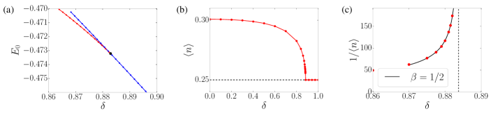
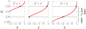
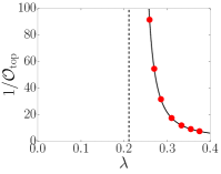
Figure 1 shows the phase diagram obtained with the infinite density matrix renormalization group (iDMRG) method White (1992); Kjäll et al. (2013). For , we have Ising critical points at , beyond which there are trivial gapped phases.
For finite , we see a large gapless phase which is entered by a Berezinskiǐ-Kosterlitz-Thouless (BKT) transition Berezinskiǐ (1972); Kosterlitz and Thouless (1973). The central charge, , is consistent with this being a Luttinger liquid (LL). This is surprising since LLs usally appear in the presence of stabilizing symmetries, such as , or at fine-tuned critical points. To better understand this phase, we study the limit in the next section.
We mention in passing that the spin- chain corresponding to is the transverse-field Ising chain with a soft constraint. Interestingly, using a nonlocal (Kramers-Wannier) transformation, this spin chain can be mapped onto the axial/anisotropic next-nearest neighbor Ising (ANNNI) chain. This mapping is also nonlocal in parameter space, e.g. mapping the limit onto a single (‘multiphase’) point. Hence, puts the ANNNI model in a new light. For example, having a gapless phase for (numerically observed in Fig. 1 and analytically argued in the following section) is equivalent to the gapless phase of the ANNNI mode having finite extent above the multiphase point, which had been debated in the literature; details are discussed in Appendix B.
Stability and symmetry in the constrained limit.—In the strong-coupling limit , the effective Hilbert space consists of all states where neighboring sites cannot both be occupied. This is an example of a Hilbert space without a tensor product structure, e.g. evidenced by its dimension asymptotically scaling as (with being the golden ratio) Moessner and Sondhi (2001). At leading order, the effective Hamiltonian is given by Eq. (2) projected into this subspace, i.e. :
| (3) |
where projects onto an empty site. (This may be dubbed the PXXP model, akin to the PXP model Turner et al. (2018, 2018); Choi et al. (2018).) The superconducting terms have disappeared! This is because they would violate the constraint. Remarkably, this model is known to be integrable and a LL for Alcaraz and Bariev (1999).
At next order in perturbation theory, the symmetry of the Hamiltonian is broken by second-nearest neighbor couplings: (see Appendix C for the complete effective Hamiltonian at this order). However, we now show that these terms do not destroy the symmetry at low energies: the gapless phase is robust for .
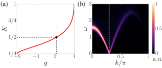
This stability can be understood from the Luttinger liquid parameter . A defining characteristic of is that it is the inverse of the scaling dimension of pair creation. Hence, if , superconducting fluctuations have a scaling dimension larger than two and are thus irrelevant in the renormalization group flow. From the Bethe ansatz solution of Eq. (3), and are related as follows Alcaraz and Bariev (1999) (see Appendix E for a derivation):
| (4) |
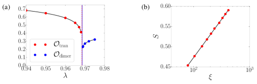
This is plotted in Fig. 2(a), with evolving from to . For , we have , avoiding the SC instability.
The model also avoids the CDW instability. It can be shown that , where is the ground state filling Alcaraz and Bariev (1999) (see also Appendix E). Hence, Eq. (4) tells us how determines the filling. In the limiting cases and , the filling is and , respectively. In between, it takes all intermediate values. This implies that the filling and the Fermi point are generically incommensurate. Hence, no matter how many times we fold the BZ, the gapless mode cannot gap out; all we need is translation symmetry with respect to some unit cell. We confirm the incommensurability of in Fig. 2(b), showing the fermionic spectral function for . This is obtained by calculating the dynamical correlation function using DMRG White and Affleck (2008); Zaletel et al. (2015).
In summary, the effective model (3) is protected against the SC instability due to and against the CDW instability due to incommensurability. Both properties are conceptually related to the constraint: the former due to the suppression of pair fluctuations, the latter due to the non-trivial optimization of ground state filling.
A nearby integrable model with soft constraint.—In the previous section, we saw that in the limit of Eq. (2), the strongly-interacting Kitaev chain becomes integrable and explicitly -symmetric. This gave us insight into the stability of the gapless phase. We now point out that although the Kitaev chain with a soft constraint is non-integrable, it can be seen as a perturbation of an integrable, -symmetric model. We use this to qualitatively explain the phase diagram obtained in Fig. 1. Note that if we remove the SC terms of Eq. (2), we obtain
| (5) |
In the constrained limit , this leads to the same effective Hamiltonian as before! In other words, for large . In particular, whenever is a Luttinger liquid phase with (with appreciable values of ), we can expect to be critical.
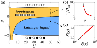
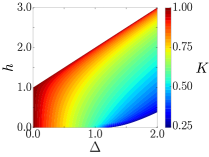
This relationship is useful since is integrable. In particular, the Jordan-Wigner transformation maps it to the paradigmatic XXZ chain in a field. Ref. Bogoliubov et al. (1986) presents the integral equations for the Luttinger liquid parameter of the XXZ chain. Numerically solving these equations, we arrive at the phase diagram in Fig. 3 (see Appendix D for details). If we perturb with -breaking terms, we expect the region with to remain gapless. This indeed qualitatively matches the gapless phase of in Fig. 1, whereas the region has flown to the gapped topological Kitaev phase.
Stability in the spin chain language through longer-range constraints.—The above demonstrated the stability of LLs in fermionic chains. However, in the hardcore boson/spin chains obtained by a Jordan-Wigner transformation, single-particle fluctuations can occur. These are considerably more effective at opening gaps: their scaling dimension is , which is relevant whenever . There are two ways out of this instability: either we enforce the parity symmetry by hand, or we introduce stronger constraints; we explore the latter.
A natural way of suppressing single-particle fluctuations is by penalizing two particles within a distance (until now ). One can then think of each particle as effectively extending over sites. If the density is not too dilute, there will be no more room for single-particle fluctuations. Such generalized constraints are softly implemented by the term . Adding this to the Kitaev or Ising chain and taking gives us a generalization of Eq. (3). In the spin chain language, we obtain
| (6) |
where the projector ensures that we remain in the constrained Hilbert space.
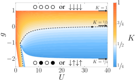
Remarkably, this model is integrable for any value of Alcaraz and Bariev (1999). It is a LL for , attaining its maximal filling at . This signals a Pokrovsky-Talapov (PT) transition into a commensurate gapped phase Pokrovsky and Talapov (1980), and as predicted by PT universality, the Luttinger liquid parameter is in this limiting case 222More generally, one can prove that in this model. Note that .. Note that if , then . More generally, one can derive the relationship between and Alcaraz and Bariev (1999):
| (7) |
(For , this reduces to Eq. (4).) This relationship is plotted in Fig. 4. We observe that for , there are indeed gapless regions where , ensuring stability against -breaking terms.
For , we can make a conceptual connection with the work of Fendley, Sengupta and Sachdev Fendley et al. (2004). They considered a model without on-site symmetry and found that when occupation was suppressed for both nearest and next-to-nearest neighbors, then there was a gapless phase of small but finite extent. This is qualitatively similar to Fig. 4, where there is a small region for which when . For , we see that this region has vastly increased to (moreover, for ). Longer-range constraints clearly stabilize the Luttinger liquid against particle and pair fluctuations.
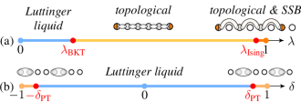
-breaking and dimerization in the nearest-neighbor-constrained Hilbert space.—Above we have shown how constraints can stabilize a LL against perturbations that break , and translation symmetry. In this last part, we explore what phases are realized when making such perturbations strong. This touches upon the question of what phases of matter can be stabilized in constrained Hilbert spaces. As our starting point, we use in Eq. (3) (i.e. ).
In the unconstrained case, breaking the symmetry of the fermionic chain yields a topological phase (a symmetry-breaking phase in the spin chain). Alternatively, introducing bond-alternation forms a symmetry-protected topological phase: the so-called Su-Schrieffer-Heeger chain in the fermionic case Su et al. (1979) (the Haldane phase in the spin language with an appropriate choice of unit cell Haldane (1983); Hida (1992)). It is natural to wonder whether these phases are also realized in the constrained Hilbert space.
First, we perturb with -breaking terms:
| (8) |
where is the second-nearest-neighbor Kitaev chain and is the projector onto the constrained Hilbert space; such a term is perturbatively generated in . The phase diagram obtained with iDMRG is shown in Fig. 5(a), where we chose . We indeed find that for large enough , the topological Kitaev chain phase is realized in the constrained Hilbert space. Interestingly, for even larger values of , the translation symmetry is spontaneously broken. (Numerical details for the critical points are found in Appendix F.) The unconstrained model would realize two decoupled Kitaev chains on even and odd sites. The constrained model , however, prefers to keep every other site (nearly) empty; the remaining sites are now unconstrained.
This is a general mechanism for realizing any unconstrained phase in the constrained Hilbert space: simply leave every other site empty. Then any state on the remaining sites trivially satisfies the constraint.
Secondly, we introduce bond-alternation to at :
| (9) |
We know that the LL is stable for small enough (see Fig. 2(b)), but Fig. 5(b) shows that it persists all the way to . At that point, there is a Pokrovsky-Talapov transition Pokrovsky and Talapov (1980) into a commensurate phase with filling (see Appendix G for details). For positive , the two ground states are symmetry protected topological (SPT) phases with respect to the remaining spatial inversion symmetry, one of which is non-trivial with protected degeneracies in its entanglement spectrum. There are no physical edge modes since inversion is broken near the boundary.
Thus, in addition to verifying the stability of the Luttinger liquid, we found various symmetry-breaking and topological phases in the constrained Hilbert space.
Conclusion.—In this work we have elucidated how soft and hard constraints in one-dimensional systems can give rise to emergent symmetry and gaplessness without fine-tuning. Experimentally verifying and exploring these gapless phases—including the longer-range constraints—is within reach Keesling et al. (2018).
A natural question is whether the same principle might also help to stabilize, e.g., Fermi liquids in higher dimensions. Or staying in one spatial dimension, one could explore larger symmetry groups and, relatedly, central charges .
An important open problem is the classification of phases in the constrained Hilbert space. Above, we have discussed how any unconstrained phase can be trivially realized in the constrained Hilbert space by breaking translation symmetry. It is natural to explore realizations that preserve translation symmetry. More exotically, might there be phases that can only be realized and stabilized in constrained Hilbert spaces—much like how enforcing symmetry vastly expanded the zoo of one-dimensional phases of matter Schnyder et al. (2008); Kitaev (2009); Ryu et al. (2010); Fidkowski and Kitaev (2011); Turner et al. (2011); Chen et al. (2011); Schuch, N. and Pérez-García, D. and Cirac, J. I. (2011)? A recent work answers a resounding and exciting yes to the latter question for the case of gapless phases Jones and Metlitski (2019).
Acknowledgements.—The authors would like to thank Dave Aasen, Henrik Dreyer, Nicola Pancotti, Maksym Serbyn and Ryan Thorngren for stimulating conversations. RV is indebted to Nick G. Jones for his insights into Luttinger liquids and for a careful reading of the manuscript. RV was supported by the German Research Foundation (DFG) through the Collaborative Research Center SFB 1143, AV is supported by a Simons Investigator Award and by the AFOSR MURI grant FA9550- 14-1-0035, and FP acknowledges the support of the DFG Research Unit FOR 1807 through grants no. PO 1370/2-1, TRR80, the European Research Council (ERC) under the European Union’s Horizon 2020 research and innovation program (grant agreement no. 771537), and the Deutsche Forschungsgemeinschaft (DFG, German Research Foundation) under Germany’s Excellence Strategy - EXC-2111 - 390814868.
References
- Bernal and Fowler (1933) J. D. Bernal and R. H. Fowler, The Journal of Chemical Physics 1, 515 (1933).
- Pauling (1935) L. Pauling, Journal of the American Chemical Society 57, 2680 (1935).
- Lieb (1967) E. H. Lieb, Phys. Rev. Lett. 18, 692 (1967).
- Baxter (1982) R. J. Baxter, Exactly solved models in statistical mechanics (Academic Press, 1982).
- Anderson (1987) P. W. Anderson, Science 235, 1196 (1987).
- Rokhsar and Kivelson (1988) D. S. Rokhsar and S. A. Kivelson, Phys. Rev. Lett. 61, 2376 (1988).
- Moessner and Raman (2008) R. Moessner and K. S. Raman, arXiv e-prints , arXiv:0809.3051 (2008), arXiv:0809.3051 [cond-mat.str-el] .
- Castelnovo et al. (2008) C. Castelnovo, R. Moessner, and S. L. Sondhi, Nature (London) 451, 42 (2008).
- Freedman et al. (2004) M. Freedman, C. Nayak, K. Shtengel, K. Walker, and Z. Wang, Annals of Physics 310, 428 (2004).
- Levin and Wen (2005) M. A. Levin and X.-G. Wen, Phys. Rev. B 71, 045110 (2005).
- Kogut (1979) J. B. Kogut, Rev. Mod. Phys. 51, 659 (1979).
- Jaksch et al. (2000) D. Jaksch, J. I. Cirac, P. Zoller, S. L. Rolston, R. Côté, and M. D. Lukin, Phys. Rev. Lett. 85, 2208 (2000).
- Weimer et al. (2010) H. Weimer, M. Müller, I. Lesanovsky, P. Zoller, and H. P. Büchler, Nature Physics 6, 382 (2010).
- Viteau et al. (2011) M. Viteau, M. G. Bason, J. Radogostowicz, N. Malossi, D. Ciampini, O. Morsch, and E. Arimondo, Phys. Rev. Lett. 107, 060402 (2011).
- Bernien et al. (2017) H. Bernien, S. Schwartz, A. Keesling, H. Levine, A. Omran, H. Pichler, S. Choi, A. S. Zibrov, M. Endres, M. Greiner, V. Vuletić, and M. D. Lukin, Nature (London) 551, 579 (2017).
- Lukin et al. (2001) M. D. Lukin, M. Fleischhauer, R. Cote, L. M. Duan, D. Jaksch, J. I. Cirac, and P. Zoller, Phys. Rev. Lett. 87, 037901 (2001).
- Urban et al. (2009) E. Urban, T. A. Johnson, T. Henage, L. Isenhower, D. D. Yavuz, T. G. Walker, and M. Saffman, Nature Physics 5, 110 (2009).
- Gaëtan et al. (2009) A. Gaëtan, Y. Miroshnychenko, T. Wilk, A. Chotia, M. Viteau, D. Comparat, P. Pillet, A. Browaeys, and P. Grangier, Nature Physics 5, 115 (2009).
- Turner et al. (2018) C. J. Turner, A. A. Michailidis, D. A. Abanin, M. Serbyn, and Z. Papic, Nature Physics 14, 745 (2018).
- Turner et al. (2018) C. J. Turner, A. A. Michailidis, D. A. Abanin, M. Serbyn, and Z. Papić, Phys. Rev. B 98, 155134 (2018).
- Choi et al. (2018) S. Choi, C. J. Turner, H. Pichler, W. W. Ho, A. A. Michailidis, Z. Papić, M. Serbyn, M. D. Lukin, and D. A. Abanin, arXiv e-prints , arXiv:1812.05561 (2018), arXiv:1812.05561 [quant-ph] .
- Fendley et al. (2004) P. Fendley, K. Sengupta, and S. Sachdev, Phys. Rev. B 69, 075106 (2004).
- Lesanovsky (2011) I. Lesanovsky, Phys. Rev. Lett. 106, 025301 (2011).
- Lesanovsky and Katsura (2012) I. Lesanovsky and H. Katsura, Phys. Rev. A 86, 041601 (2012).
- Lesanovsky (2012) I. Lesanovsky, Phys. Rev. Lett. 108, 105301 (2012).
- Chepiga and Mila (2019) N. Chepiga and F. Mila, Phys. Rev. Lett. 122, 017205 (2019).
- Giudici et al. (2019) G. Giudici, A. Angelone, G. Magnifico, Z. Zeng, G. Giudice, T. Mendes-Santos, and M. Dalmonte, arXiv e-prints , arXiv:1901.10850 (2019), arXiv:1901.10850 [cond-mat.quant-gas] .
- Schnyder et al. (2008) A. P. Schnyder, S. Ryu, A. Furusaki, and A. W. W. Ludwig, Phys. Rev. B 78, 195125 (2008).
- Kitaev (2009) A. Kitaev, AIP Conference Proceedings 1134, 22 (2009).
- Ryu et al. (2010) S. Ryu, A. P. Schnyder, A. Furusaki, and A. W. W. Ludwig, New Journal of Physics 12, 065010 (2010).
- Fidkowski and Kitaev (2011) L. Fidkowski and A. Kitaev, Phys. Rev. B 83, 075103 (2011).
- Turner et al. (2011) A. M. Turner, F. Pollmann, and E. Berg, Phys. Rev. B 83, 075102 (2011).
- Chen et al. (2011) X. Chen, Z.-C. Gu, and X.-G. Wen, Phys. Rev. B 83, 035107 (2011).
- Schuch, N. and Pérez-García, D. and Cirac, J. I. (2011) Schuch, N. and Pérez-García, D. and Cirac, J. I., Phys. Rev. B 84, 165139 (2011).
- Kitaev (2001) A. Y. Kitaev, Physics-Uspekhi 44, 131 (2001).
- Note (1) Note that commutes with for open boundaries.
- Alcaraz and Bariev (1999) F. C. Alcaraz and R. Z. Bariev, arXiv e-prints , cond-mat/9904042 (1999), arXiv:cond-mat/9904042 [cond-mat.stat-mech] .
- Calabrese and Cardy (2004) P. Calabrese and J. Cardy, Journal of Statistical Mechanics: Theory and Experiment 2004, P06002 (2004).
- Pollmann et al. (2009) F. Pollmann, S. Mukerjee, A. M. Turner, and J. E. Moore, Phys. Rev. Lett. 102, 255701 (2009).
- White (1992) S. R. White, Phys. Rev. Lett. 69, 2863 (1992).
- Kjäll et al. (2013) J. A. Kjäll, M. P. Zaletel, R. S. K. Mong, J. H. Bardarson, and F. Pollmann, Phys. Rev. B 87, 235106 (2013).
- Berezinskiǐ (1972) V. L. Berezinskiǐ, Soviet Journal of Experimental and Theoretical Physics 34, 610 (1972).
- Kosterlitz and Thouless (1973) J. M. Kosterlitz and D. J. Thouless, Journal of Physics C: Solid State Physics 6, 1181 (1973).
- Moessner and Sondhi (2001) R. Moessner and S. L. Sondhi, Phys. Rev. B 63, 224401 (2001).
- White and Affleck (2008) S. R. White and I. Affleck, Phys. Rev. B 77, 134437 (2008).
- Zaletel et al. (2015) M. P. Zaletel, R. S. K. Mong, C. Karrasch, J. E. Moore, and F. Pollmann, Phys. Rev. B 91, 165112 (2015).
- Bogoliubov et al. (1986) N. Bogoliubov, A. Izergin, and V. Korepin, Nuclear Physics B 275, 687 (1986).
- Pokrovsky and Talapov (1980) V. Pokrovsky and A. Talapov, Solid State Communications 33, 749 (1980).
- Note (2) More generally, one can prove that in this model. Note that .
- Su et al. (1979) W. P. Su, J. R. Schrieffer, and A. J. Heeger, Phys. Rev. Lett. 42, 1698 (1979).
- Haldane (1983) F. D. M. Haldane, Phys. Rev. Lett. 50, 1153 (1983).
- Hida (1992) K. Hida, Phys. Rev. B 45, 2207 (1992).
- Keesling et al. (2018) A. Keesling, A. Omran, H. Levine, H. Bernien, H. Pichler, S. Choi, R. Samajdar, S. Schwartz, P. Silvi, S. Sachdev, P. Zoller, M. Endres, M. Greiner, V. Vuletic, and M. D. Lukin, arXiv e-prints , arXiv:1809.05540 (2018), arXiv:1809.05540 [quant-ph] .
- Jones and Metlitski (2019) R. A. Jones and M. A. Metlitski, arXiv e-prints , arXiv:1902.05957 (2019), arXiv:1902.05957 [cond-mat.str-el] .
- Peschel and Emery (1981) I. Peschel and V. J. Emery, Zeitschrift für Physik B Condensed Matter 43, 241 (1981).
- Chandra and Dasgupta (2007a) A. K. Chandra and S. Dasgupta, Phys. Rev. E 75, 021105 (2007a).
- Beccaria et al. (2007) M. Beccaria, M. Campostrini, and A. Feo, Phys. Rev. B 76, 094410 (2007).
- Nagy (2011) A. Nagy, New Journal of Physics 13, 023015 (2011).
- Villain and Bak (1981) J. Villain and P. Bak, Journal de Physique 42, 657 (1981).
- Shirahata and Nakamura (2001) T. Shirahata and T. Nakamura, Phys. Rev. B 65, 024402 (2001).
- Derian et al. (2006) R. Derian, A. Gendiar, and T. Nishino, Journal of the Physical Society of Japan 75, 114001 (2006).
- Chandra and Dasgupta (2007b) A. K. Chandra and S. Dasgupta, Journal of Physics A: Mathematical and Theoretical 40, 6251 (2007b).
- Shirakura et al. (2014) T. Shirakura, F. Matsubara, and N. Suzuki, Phys. Rev. B 90, 144410 (2014).
- Matsubara et al. (2017) F. Matsubara, T. Shirakura, and N. Suzuki, Phys. Rev. B 95, 174409 (2017).
- Kato (1949) T. Kato, Progress of Theoretical Physics 4, 514 (1949).
- Takahashi (1977) M. Takahashi, Journal of Physics C: Solid State Physics 10, 1289 (1977).
- Cabra et al. (1998) D. C. Cabra, A. Honecker, and P. Pujol, Phys. Rev. B 58, 6241 (1998).
Appendix A Fermionic and spin models
For clarity and completeness, here we include all the hardcore bosonic/spin models that are related to the fermionic models of the main text via the Jordan-Wigner transformation:
| (A1) | ||||
| (A2) | ||||
| (A3) |
(We will use to represent the spin- Pauli matrices, i.e. .) In particular, the Kitaev chain, , takes the same form in terms of the hardcore bosons defined by the above Jordan-Wigner transformation: , known as the Ising chain.
A.1 The Kitaev/Ising chain with a soft constraint
In the main text we considered the following fermionic model:
| (A4) |
The corresponding spin- model (ignoring overall additive constants) is:
| (A5) |
A.2 The Kitaev/Ising chain with a hard constraint
Taking the limit of the above model, we obtained the following effective model in the constrained Hilbert space:
| (A6) |
The corresponding spin- chain is:
| (A7) |
Here projects onto a down spin.
At next order in , the fermionic model has its symmetry explicitly broken by . In the spin model, this is .
A.3 The free fermion/XY chain with a soft constraint
The aforementioned effective model had an explicit symmetry. In fact, it also arises as the hard-constraint limit of the following symmetric fermionic model, as considered in the main text:
| (A8) |
The corresponding spin- chain is:
| (A9) |
Writing , one can see that the latter is equivalent to the XXZ chain with and .
A.4 -breaking and dimerization in the constrained limit
A.4.1 -breaking
| (A10) | ||||
| (A11) |
A.4.2 dimerization
| (A12) | ||||
| (A13) |
Appendix B Relation to the axial/anisotropic next-nearest-neighbor Ising (ANNNI) model
We can rewrite the model appearing in the main text as follows (also see Eq. (A5)):
| (A14) | ||||
| (A15) |
If we drop the constant and perform a Kramers-Wannier transformation,
| (A16) |
then we obtain
| (A17) | ||||
| (A20) |
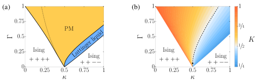
We thus see that the model is equivalent to the ANNNI model (where we have used its traditional parametrization). This mapping allows us to plot the phase diagram in Fig. 1 (of the main text) in terms of and . This is shown in Fig. A1(a). Moreover, we show the -enhanced model in Fig. A1(b), which is the analogue of Fig. 3 of the main text. (Explicitly, the integrable -enhanced model is , where the generator of the symmetry is .)
Despite the (soft-)constrained model in the main text mapping to the ANNNI model, there are two important differences in the representation of these models, with distinct physical consequences.
Firstly, they are related by a non-local (Kramers-Wannier) transformation. Hence, whereas the model in the main text has emergent symmetries whose charges are local, the gapless phase in the ANNNI model has a non-local symmetry. (More precisely, its generator is an matrix product operator, and operators with the smallest possible charge are non-local string operators.) Conceptually, this makes the model in the main text (and its phenomenology, such a stable gapless phases) arguably easier to understand. Quantitatively, it for example affects the oscillations of the correlation functions: in the model in the main text, the correlation functions do not have (sign-changing) oscillations. For the corresponding ANNNI model, however, the correlations (in addition to having a different scaling dimension), pick up large oscillations determined by the wavevector. (Relatedly, the values of shown in Fig. A1(b) need to be interpreted with care: strictly speaking, they refer to the values of the Luttinger liquid parameter prior to the Kramers-Wannnier transformation; see Fig. 3 of the main text.)
Secondly, the parameters in the Hamiltonian are also non-locally related. In particular, the interesting and integrable limit with finite, is mapped to a single point of the ANNNI phase diagram: and . This is yet another way in which the model of the main text is easier to analyze than the ANNNI model. In particular, there are two hotly-debated questions about the ANNNI model which are straightforwardly addressed in terms of the model of the main text:
-
1.
Does the gapless phase of the ANNNI model have a finite extent at ? This is equivalent to asking whether the model of the main text is gapless for and large. We answered this in the positive by first using Bethe ansatz to show that the limit is gapless, and subsequently arguing that this is stable for finite (but large) due to . Moreover, we numerically found that for , the model was gapless for ; this means that the ANNNI model is gapless for and .
-
2.
Does the PM phase reach ? A perturbative calculation around the and limit seemingly proved that the PM phase terminates at a finite value of Chandra and Dasgupta (2007a). However, subsequent DMRGBeccaria et al. (2007) and iDMRGNagy (2011) works could not corroborate this. Indeed, an earlier analytical work by Peschel and Emery already showed that there is an exactly solvable line in the PM phase that terminates at the and point Peschel and Emery (1981) (dotted line in Fig. A1(a)).
We now resolve this paradox. The claim in Ref. Chandra and Dasgupta (2007a) was based on finding that there are only two critical emanating from the and point at leading-order in . But at this order, the system develops an explicit symmetry; at this level Fig. A1(a) and Fig. A1(b) are indistinguishable, and the latter indeed only has two critical lines emerging from this point. The catch is that part of the gapless phase opens up a gap at the next-to-leading order in , becoming the PM phase. (We have discussed this in detail in the main text, relating it to the value of the Luttinger liquid parameter.) In conclusion, there are three critical lines (as shown in Fig. A1(a)), with the PM phase reaching the multi-phase point.
Lastly, we would be remiss not touching upon the early seminal work on the two-dimensional classical ANNNI model. In particular, in 1981, Villain and Bak realized that near and at low temperature (related to small ), the systems develops an effective symmetry Villain and Bak (1981). Moreover, in that same work, they used a free-fermion approach where they derived formulas for exponents in the algebraic phase which are in close agreement with those quoted in our main text. We can now interpret this as Villain and Bak having realized the solvability of the (hard-)constrained model, apparently almost two decades before it was explicitly discovered Alcaraz and Bariev (1999). Nevertheless, it is not entirely clear to what extent these approaches coincide, especially since the (hard-)constrained model is not a free-fermion model (albeit a projection of one). It could be interesting to explore these relationships further. Relatedly, note that the two-dimensional classical and one-dimensional quantum model are not trivially related. Indeed, whereas the gapless phase of the 1D quantum ANNNI model was established early on, it had been claimed that in the 2D classical model this phase might be of vanishing width Shirahata and Nakamura (2001); Derian et al. (2006); Chandra and Dasgupta (2007b). This issue was only settled in recents years, concluding that there is an extended phase Shirakura et al. (2014); Matsubara et al. (2017).
Appendix C Perturbation theory
Here we calculate the effective Hamiltonian for the Kitaev/Ising chain with a soft constraint in the limit where .
We set up the perturbation theory (in the bosonic language) as follows: with and . Let be the projector onto the constrained Hilbert space.
For large , we can write down an effective Hamiltonian: . For , we have . We know , which gives us
| (A21) |
Appendix D Luttinger liquid parameter in the XXZ chain
We start from the model of the main text, parameterizing it in terms of and . Using the Jordan-Wigner transformation (see Eqs. (A1)–(A3)), we map it to the XXZ chain:
| (A24) | ||||
| (A25) |
The integral equations which specify its Luttinger liquid parameter were derived in Ref. Bogoliubov et al. (1986). By numerically solving these, we obtain the data in Fig. A2. For completeness, we reproduce the integral equations here, following the notation of Ref. Cabra et al. (1998). This will also allow us to derive simple analytic relationships in the constrained limit in the next section. In particular, we present the formulas for . (For , the same formulas apply with all trigonometric functions replaced by their hyperbolic counterparts and vice versa.)
We consider and the filling to be fixed. (We will determine the corresponding field .) We then define the following two kernels:
| (A26) |
In terms of these, we define and by the following two integral equations:
| (A27) |
The Luttinger liquid parameter is given by where . The field is determined by , where .
Appendix E Analytic relationships in the limit
As , we see from Eq. (A26) that . Hence, , whose solution is . In particular, is constant, such that the condition implies that . Equating these two solutions gives us .
Similarly, is also constant, with the solution from the integral equation being . We conclude that the Luttinger liquid parameter , as claimed in the main text. (It will also be useful to note that . Note that for , we have .)
To determine the field , we note that for large , we can approximate the integral equation for as where we used that . Integrating both sides of the integral equation and defining , we obtain , i.e. . Thus,
| (A28) |
In conclusion, we derive that
| (A29) |
Given the identification of the models in the main text, i.e. and , we conclude that in the limit, we have , in agreement with what was claimed in the main text.
Appendix F Criticality in constrained model with -breaking terms
Here we analyze of the main text, setting :
| (A30) |
F.1 Berezinskii-Kosterlitz-Thouless (BKT) universality as
From fitting how the order parameter goes to zero, using the BKT formula (see main text), we obtain (see Fig. A3).
F.2 Ising criticality as
We first locate the critical point by looking at order parameters. For large , the state spontaneously breaks translation symmetry, for which we can define the order parameter , which vanishes at the critical point as shown in Fig. A4(a). There are only very few points accessible (given the narrow window of the phase), from which we extract an approximate scaling dimension .
Considering that the phase is much more stable when coming from the other side, we would like to look at the expectation value of the corresponding disorder operator (i.e. the operator which can be regarded as being condensed in the symmetry-preserving phase). For this we choose the operator which implements a shift on half the system, as shown in Fig. A5. This vanishes at the same point as shown in Fig. A4(a), which gives the reliable value . The extracted critical exponent is .
The values of the critical exponents, and (the latter being more reliable than the former), are approximately consistent with the CFT prediction for the Ising universality class, where for both the order and disorder parameters. In addition, we extract the central charge from entanglement scaling, shown in Fig. A4(b). This gives a fit , in close agreement with the predicted value .
Appendix G Criticality in constrained model with bond-alternation
Here we analyze of the main text.
G.1 Pokrovsky-Talapov (PT) criticality as
There is a PT transition at . This is analzed in Fig. A6. Note that this transition looks first order when coming from the right; this is also evidenced in Fig. A6(a) where adiabatically following the ground state for reaches a metastable state for . Nevertheless, the transition is continuous, and indeed the ground state energy from the left is tangent to the blue line in Fig. A6(a).
Similarly, on the one hand, coming from , the order parameter has a discontinuity at the transition (not shown), whilst on the other hand, approaching from the left, physical observables will be continuous. This is shown in Fig. A6(b), where we track the (incommensurate) ground state filling. In Fig. A6(c) we confirm that this behavior is consistent with the critical exponent predicted for the PT universality class.