The ALMA Spectroscopic Survey in the HUDF: the molecular gas content of galaxies
and tensions with IllustrisTNG and the Santa Cruz SAM

Abstract

The ALMA Spectroscopic Survey in the Hubble Ultra Deep Field (ASPECS) provides new constraints for galaxy formation models on the molecular gas properties of galaxies. We compare results from ASPECS to predictions from two cosmological galaxy formation models: the IllustrisTNG hydrodynamical simulations and the Santa Cruz semi-analytic model (SC SAM). We explore several recipes to model the H₂ content of galaxies, finding them to be consistent with one another, and take into account the sensitivity limits and survey area of ASPECS. For a canonical CO–to–H₂ conversion factor of $\alpha_{\rm CO}=3.6\,\rm{M}_{\odot}/(\rm{K}\,\rm{km/s}\,\rm{pc}^{2})$ the results of our work include: (1) the H₂ mass of $z>1$ galaxies predicted by the models as a function of their stellar mass is a factor of 2–3 lower than observed; (2) the models do not reproduce the number of H₂-rich ($M_{\rm H2}>3\times 10^{10}\,\rm{M}_{\odot}$) galaxies observed by ASPECS; (3) the H₂ cosmic density evolution predicted by IllustrisTNG (the SC SAM) is in tension (only just agrees) with the observed cosmic density, even after accounting for the ASPECS selection function and field-to-field variance effects. The tension between models and observations at $z>1$ can be alleviated by adopting a CO–to–H₂ conversion factor in the range $\alpha_{\rm CO}=2.0-0.8\,\rm{M}_{\odot}/(\rm{K}\,\rm{km/s}\,\rm{pc}^{2})$. Additional work on constraining the CO–to–H₂ conversion factor and CO excitation conditions of galaxies through observations and theory will be necessary to more robustly test the success of galaxy formation models.

1 Introduction

Surveys of large fields in the sky have been instrumental for our understanding of galaxy formation and evolution. A pioneering survey was carried out with the Hubble Space Telescope (HST, Williams et al., 1996), pointing at a region in the sky now known as the Hubble Deep Field (HDF). Ever since, large field surveys have been carried out at X-ray, optical, infrared, submillimeter (sub-mm) continuum, and radio wavelengths. These efforts have revealed the star-formation (SF) history of our Universe, quantified the stellar build-up of galaxies, and have been used to derive galaxy properties such as stellar masses, star-formation rates (SFR), morphologies, and sizes over cosmic time (e.g., Madau & Dickinson, 2014). One of the most well known results obtained is that the SF history of our Universe peaked at redshifts $z\sim 2-3$, after which it dropped to its present-day value (e.g., Lilly et al., 1995; Madau et al., 1996; Hopkins, 2004; Hopkins & Beacom, 2006, for a recent review see Madau & Dickinson 2014).

Although the discussed efforts have shed light on the evolution of galaxy properties such as stellar mass, morphology, and SF, similar studies focusing on the gas content, the fuel for star formation, have lagged behind. New and updated facilities operating in the millimeter and radio waveband such as the Atacama Large (sub-)Millimeter Array (ALMA), NOrthern Extended Millimeter Array (NOEMA), and the Jansky Very Large Array (JVLA) have now made a survey of cold gas in our Universe feasible. A first pilot to develop the necessary techniques was performed with the Plateau de Bure Interferometer (Decarli et al., 2014; Walter et al., 2014). This was followed by the first search for emission lines, mostly carbon monoxide (¹²CO, hereafter CO) using ALMA, focusing on a small ($\sim$1 arcmin²) region within the Hubble Ultra Deep Field (HUDF, Walter et al., 2016; Decarli et al., 2016). This effort is currently extended (4.6 arcmin²) as part of ‘The ALMA Spectroscopic Survey in the Hubble Ultra Deep Field’ (ASPECS, Walter et al., 2016; Gonzales et al., 2019; Decarli et al., 2019). Among other goals, this survey aims to detect CO emission and fine-structure lines of carbon over cosmic time in the HUDF. The CO emission is used as a proxy for the molecular hydrogen gas content of galaxies (through a CO–to–H₂ molecular gas conversion factor). A complementary survey, COLDZ, has been carried out with the JVLA in GOODS-North and COSMOS (Pavesi et al., 2018; Riechers et al., 2018). The area covered on the sky by COLDZ is larger compared to ASPECS, but it is shallower (and focuses on CO J$=$1–0 instead of the higher rotational transitions targeted by ASPECS).

Surveys of a field on the sky are complementary to surveys targeting galaxies based on some pre-selection. First of all, a survey without a pre-selection of targets allows one to detect classes of galaxies that would have potentially been missed in targeted surveys because they do not fulfil the selection criteria. Second, these surveys are the perfect tool to measure the number densities of different classes of galaxies. With this in mind, one of the main science goals of ASPECS is to quantify the H₂ mass function and H₂ cosmic density of the Universe over time.

Surveys focusing on the gas content of galaxies and our Universe provide an important constraint and additional challenge for theoretical models of galaxy formation. Theoretical models can be used to estimate limitations in the observations (e.g., field-to-field variance, selection functions) and to put the observational results into a broader context (gas baryon cycle, galaxy evolution). On the other hand, observational constraints help the modelers in better understanding the physics relevant for galaxy (and gas) evolution (such as feedback and star-formation recipes), and they can serve as benchmarks to understand the strengths/limitations of models.

During the last decade a large number of groups have implemented the modeling of H₂ in post-processing or on-the-fly in hydrodynamic (e.g., Popping et al., 2009; Christensen et al., 2012; Kuhlen et al., 2012; Thompson et al., 2014; Lagos et al., 2015; Marinacci et al., 2017; Diemer et al., 2018; Stevens et al., 2018) and in (semi-)analytic models (e.g., Obreschkow & Rawlings, 2009; Dutton et al., 2010; Fu et al., 2010; Lagos et al., 2011; Krumholz et al., 2012; Popping et al., 2014b; Xie et al., 2017; Lagos et al., 2018). Most of these models use metallicity- or pressure-based recipes to separate the cold interstellar medium (ISM) into an atomic (Hi) and molecular (H₂) component. The pressure-based recipe builds upon the empirically determined relation between the mid-plane pressure acting on a galaxy disc and the ratio between atomic and molecular hydrogen (Blitz & Rosolowsky, 2004, 2006; Leroy et al., 2008). The physical motivation for the correlation between mid-plane pressure and molecular hydrogen mass fraction was first presented in Elmegreen (1989). The metallicity-based recipes (where the metallicity is a proxy for the dust grains that act as a catalyst for the formation of H₂) are often based on work presented in Gnedin & Kravtsov (2011) or Krumholz and collaborators (Krumholz et al., 2008, 2009a; McKee & Krumholz, 2010; Krumholz, 2013). Gnedin & Kravtsov (2011) used high-resolution simulations including chemical networks to derive fitting functions that relate the H₂ fraction of the ISM to the gas surface density of galaxies on kpc scales, the metallicity, and the strength of Ultraviolet (UV) radiation field. Krumholz et al. (2009a) presented analytic models for the formation of H₂ as a function of total gas density and metallicity, supported by numerical simulations with simplified geometries (Krumholz et al., 2008, 2009a). This work was further developed in Krumholz (2013).

In this paper we will compare predictions for the H₂ content of galaxies by the IllustrisTNG (the next generation) model (Weinberger et al., 2017; Pillepich et al., 2018a) and the Santa Cruz semi-analytic model (SC SAM, Somerville & Primack, 1999; Somerville et al., 2001) to the results from the ASPECS survey. We will specifically try to quantify the success of these different galaxy formation evolution models in reproducing the observations by accounting for sensitivity limits, field-to-field variance effects, and systematic theoretical uncertainties. We will furthermore use these models to assess the importance of field-to-field variance and the ASPECS selection functions on the conclusions drawn from the survey. We encompass the systematic uncertainties in the modeling of H₂ by employing three different prescriptions to calculate the amount of molecular hydrogen.

IllustrisTNG is a cosmological, large-scale gravity+magnetohydrodynamical simulation based on the moving mesh code AREPO (Springel, 2010). The SC SAM does not solve for the hydrodynamic equations, but rather uses analytical recipes to describe the flow of baryons between different ‘reservoirs’ (hot gas, cold gas making up the interstellar medium, ejected gas, and stars). Both models include prescriptions for physical processes such as the cooling and accretion of gas onto galaxies, star-formation, stellar and black hole feedback, chemical enrichment, and stellar evolution.

Although these two models are different in nature and have different strengths and disadvantages, they both reasonably reproduce some of the key observables of the galaxy population in our local Universe, such as the galaxy stellar mass function, sizes, and SFR of galaxies (at least at low redshifts). The different nature of these two models probes the systematic uncertainty across models when these are used to interpret observations. Furthermore, any shared successes or problems of these two models may point to a general success/misunderstanding of galaxy formation theory rather than model dependent uncertainties.

This paper is organised as follows. In Section 2 we briefly present IllustrisTNG, the SC SAM, and the implementation of the various H₂ recipes. We provide a brief overview of ASPECS in Section 3. In Section 4 we present the predictions by the different models and how these compare to the results from ASPECS. We discuss our results in Section 5 and present a short summary and our conclusions in Section 6. Throughout this paper we assume a Chabrier stellar initial mass function (IMF; Chabrier, 2003) in the mass range 0.1–100 $\rm{M}_{\odot}$ and adopt a cosmology consistent with the recent Planck results (Planck Collaboration et al., 2016, $\Omega_{m}=0.31,\,\Omega_{\Lambda}=0.69,\,\Omega_{b}=0.0486,\,h=0.677,\,\sigma_{8}=0.8159,\,n_{s}=0.97$). All presented gas masses (model predictions and observations) are pure hydrogen masses (do not include a correction for helium).

2 Description of the models

2.1 IllustrisTNG

In this paper we use and analyze the TNG100 simulation, a $\sim$(100 Mpc$)^{3}$ cosmological volume simulated with the code AREPO (Springel, 2010) within the IllustrisTNG project (Pillepich et al., 2018b; Naiman et al., 2018; Nelson et al., 2018a; Springel et al., 2018; Marinacci et al., 2018). The IllustrisTNG model is a revised version of the Illustris galaxy formation model (Vogelsberger et al., 2013; Torrey et al., 2014). TNG100 evolves cold dark matter (DM) and gas from early times to $z=0$ by solving for the coupled equations of gravity and magneto-hydrodynamics (MHD) in an expanding Universe (in a standard cosmological scenario, Planck Collaboration et al. 2016) while including prescriptions for star formation, stellar evolution and hence mass and metal return from stars to the interstellar medium (ISM), gas cooling and heating, feedback from stars and feedback from supermassive black holes (see Weinberger et al., 2017; Pillepich et al., 2018a, for details on the IllustrisTNG model).

At $z=0$, TNG100 samples many thousands of galaxies above $M_{*}\simeq 10^{10}\,\rm{M}_{\odot}$ in a variety of environments, including for example ten massive clusters above $M\simeq 10^{14}\,\rm{M}_{\odot}$ (total mass). The mass resolution of the simulation is uniform across the simulated volume (about $7.5\times 10^{6}\rm{M}_{\odot}$ for DM particles and $1.4\times 10^{6}\,\rm{M}_{\odot}$ for both gas cells and stellar particles). The gravitational forces are softened for the collisionless components (DM and stars) at about 700 pc at $z=0$, while the gravitational softening of the gas elements is adaptive and can be as small as $\sim 280$ pc. The spatial resolution of the hydrodynamics is fully adaptive, with smaller gas cells at progressively higher densities: in the star forming regions of galaxies, the average gas-cell size in TNG100 is about 355 pc (see table A1 in Nelson et al., 2018a, for more details).

The TNG100 box (or TNG, for brevity, throughout this paper) is a rerun of the original Illustris simulation (Vogelsberger et al., 2014a, b; Genel et al., 2014; Sijacki et al., 2015) with updated and new aspects of the galaxy-physics model, including – among others – MHD, modified galactic winds, and a new kinetic, black hole-driven wind feedback model. Importantly for this paper, in the Illustris and IllustrisTNG frameworks, gas is converted stochastically into stellar particles following the two-phase ISM model of Springel & Hernquist (2003): when a gas cell exceeds a density threshold ($n_{\rm H}\simeq 0.1$cm^-3), it is dubbed star forming, irrespective of its metallicity. This model prescribes that low-temperature and high-density gas (below about $10^{4}$ K and above the star-formation density threshold) is placed on an equation of state between e.g. temperature and density, meaning that the multi-phase nature of the ISM at higher densities (or colder temperatures) is assumed, rather than hydrodynamically resolved. In these simulations, the production and distribution of nine chemical elements is followed (H, He, C, N, O, Ne, Mg, Si, and Fe) but no distinction is made between atomic and molecular phases, which hence need to be modeled in post processing for the purposes of this analysis (see subsequent sections). Gas radiatively cools in the presence of a spatially uniform, redshift-dependent, ionizing UV background radiation field (Faucher-Giguère et al., 2009), including corrections for self-shielding in the dense ISM but neglecting local sources of radiation. Metal-line cooling and the effects of a radiative feedback from supermassive black holes are also taken into account in addition to energy losses induced by two-body processes (collisional excitation, collisional ionization, recombination, dielectric recombination and free-free emission) and inverse Compton cooling off the CMB.

While a certain degree of freedom is unavoidable in these models (mostly owing to the subgrid nature of a subset of the physical ingredients), their parameters are chosen to obtain a reasonable match to a small set of observational, galaxy-statistics results. For IllustrisTNG, these chiefly included the current baryonic mass content of galaxies and haloes and the galaxy stellar mass function at $z=0$ (see Pillepich et al., 2018a, for details). The IllustrisTNG outcome is consistent with a series of other observations, including the galaxy stellar mass functions at $z\lesssim 4$ (Pillepich et al., 2018b), the galaxy color bimodality observed in the Sloan Digital Sky Survey (Nelson et al., 2018a), the large-scale spatial clustering of galaxies also when split by galaxy colors (Springel et al., 2018), the gas-phase oxygen abundance and distribution within (Torrey et al., 2017) and around galaxies (Nelson et al., 2018b), the metallicity content of the intra-cluster medium (Vogelsberger et al., 2018), and the average trends, evolution, and scatter of the galaxy stellar size-mass relation at $z\lesssim 2$ (Genel et al., 2018). Thanks to such general validations of the model, we can use the IllustrisTNG galaxy population as a plausible synthetic dataset for further studies, particularly at the intermediate and high redshifts that are probed by ASPECS and that had not been considered for the model development (the gas mass fraction within galaxies were not used to constrain the model, particularly at high redshifts, which makes the current exploration interesting).

2.1.1 Input parameters for H₂ recipes in IllustrisTNG

In order to obtain the molecular gas content of simulated galaxies (see Section 2.3), we employ a number of approaches to calculate the molecular hydrogen fraction $f_{\rm H2}$ ($=M_{\rm H2}/M_{\rm Hydrogen}$) of gas cells within the simulation. The gas cells represent a mixture of Hydrogen, Helium, and metals. Although in the TNG calculations the fraction of hydrogen is tracked on a gas cell by cell basis, this is not always stored in the output data. Namely, the Hydrogen fraction is stored only in 20 of 100 snapshots (in the so-called full snapshots) and not for all the redshifts we intend to study. For these reasons, we simply assume a hydrogen fraction for the gas cells of $f_{\rm H}=0.76$.

Gas surface density

Some of the recipes employed to compute the molecular hydrogen fraction of the cold gas depend on the cold gas surface density. To calculate the gas surface density of a gas cell we multiply its gas density with the characteristic Jeans length belonging to that cell (following e.g., Lagos et al., 2015; Marinacci et al., 2017). The Jeans length $\lambda_{\rm J}$ is calculated as

$$\lambda_{\rm J}=\sqrt{\frac{c^{2}_{\rm s}}{G\rho}}=\sqrt{\frac{\gamma(\gamma-1)u}{G\rho}},$$ (1)

where $c_{\rm s}$ is the sound speed of the gas, $G$ and $\rho$ represent the gravitational constant and total gas density of a cell, respectively, $u$ the internal energy of the gas cell, and $\gamma=5/3$ the ratio of heat capacities. In the case of star-forming cells the internal energy represents a mix between the hot ISM and star-forming gas. For these cells we take the internal energy to be $T_{\rm SF}=1000\,\rm{K}$ (Springel & Hernquist, 2003; Marinacci et al., 2017).

The hydrogen gas surface density of each cell is then calculated as

$$\Sigma_{\rm H}=f_{\rm H}f_{\rm neutral,H}\lambda_{\rm J}\rho,$$ (2)

where $f_{\rm neutral,H}$ marks the fraction of hydrogen in a gas cell that is neutral (i.e., atomic or molecular). We assume $f_{\rm neutral,H}=1.0$ for star-forming cells, whereas we adopt the value suggested from IllustrisTNG for $f_{\rm neutral,H}$ for non star-forming cells.

Radiation field

For a subset of the employed recipes the molecular hydrogen fraction also depends on the local UV radiation field $G_{0}$. The local UV radiation field $G_{0}$ impinging on the gas cells is calculated differently for star-forming and non-star-forming cells. For star-forming cells we scale $G_{0}$ with the local SFR surface density ($\Sigma_{\rm SFR}$, calculated by multiplying the star-formation rate density of each cell by the Jeans length) such that

$$G_{0}=\frac{\Sigma_{\rm SFR}}{\Sigma_{\rm SFR,MW}},$$ (3)

where $\Sigma_{\rm SFR,MW}=0.004\,\rm{M}\,\rm{yr}^{-1}\,\rm{kpc}^{-2}$ is the local SFR surface density in the MW (Robertson & Kravtsov, 2008). We note that the local value for the MW SFR surface density is somewhat uncertain, varying in the range (1 – 7) $\times 10^{-3}\,\rm{M}_{\odot}\,\rm{yr}^{-1}\,\rm{kpc}^{-2}$ (Miller & Scalo, 1979; Bonatto & Bica, 2011). We scale the UV radiation field for non-star-forming cells as a function of the time-dependent Hi heating rate from Faucher-Giguère et al. (2009) at 1000 Å. Diemer et al. (2018) adopted a different approach to calculate the UV radiation field impinging on every gas cell by propagating the UV radiation from star-forming particles to its surroundings, accounting for dust absorption. The median difference in the predicted H₂ mass by Diemer et al. and our method is 15 % for galaxies with H₂ masses more massive than $10^{9}\,\rm{M}_{\odot}$ at the redshifts that are relevant for ASPECS (at $z=0$ this is $\sim 40$ % for the GK method).

Dust

The dust abundance of the cold gas in terms of the MW dust abundance $D_{\rm MW}$ is assumed to be equal to the gas-phase metallicity expressed in solar units, i.e., $D_{\rm MW}=Z/Z_{\odot}$. Both observations and simulations have demonstrated that this scaling is appropriate over a large range of gas-phase metallicities ($Z\geq 0.1\,Z_{\odot}$, Rémy-Ruyer et al., 2014; McKinnon et al., 2017; Popping et al., 2017a).

2.2 Santa Cruz semi-analytic model

The SC semi-analytic galaxy formation model was first presented in Somerville & Primack (1999) and Somerville et al. (2001). Updates to this model were described in Somerville et al. (2008, S08), Somerville et al. (2012), Popping et al. (2014b, PST14), Porter et al. (2014), and Somerville et al. (2015, SPT15). The model tracks the hierarchical clustering of dark matter haloes, shock heating and radiative cooling of gas, SN feedback, star formation, active galactic nuclei (AGN) feedback (by quasars and radio jets), metal enrichment of the interstellar and intracluster media, disk instabilities, mergers of galaxies, starbursts, and the evolution of stellar populations. PST14 and SPT15 included new recipes that track the amount of ionized, atomic, and molecular hydrogen in galaxies and included a molecular hydrogen based star-formation recipe. The SC SAM has been fairly successful in reproducing the local properties of galaxies such as the stellar mass function, gas fractions, gas mass function, SFRs, and stellar metallicities, as well as the evolution of the galaxy sizes, quenched fractions, stellar mass functions, dust content, and luminosity functions (Somerville et al., 2008, 2012; Porter et al., 2014; Popping et al., 2014a; Brennan et al., 2015; Popping et al., 2016, 2017a; Yung et al., 2018, PST14, SPT15).

The semi-analytic framework essentially describes the flow of material between different types of reservoirs. All galaxies form within a dark matter halo. There are three reservoirs for gas; the “hot” gas that is assumed to be in a quasi-hydrostatic spherical configuration throughout the virial radius of the halo; the “cold” gas in the galaxy, assumed to be in a thin disk; and the “ejected” gas which is gas that has been heated and ejected from the halo by stellar winds. Differential equations describe the movement of gas between these three reservoirs. As dark matter halos grow in mass, pristine gas is accreted from the intergalactic medium into the hot halo. A cooling model is used to calculate the rate at which gas accretes from the hot halo into the cold gas reservoir, where it becomes available to form stars. Gas participating in star formation is removed from the cold gas reservoir and locked up in stars. Gas can furthermore be removed from the cold gas reservoir by stellar and AGN-driven winds. Part of the gas that is ejected by stellar winds is returned to the hot halo, whereas the rest is deposited in the “ejected” reservoir. The fraction of gas that escapes the hot halo is calculated as a function of the virial velocity of the progenitor galaxy (see S08 for more detail). Gas “re-accretes” from the ejected reservoir back into the hot halo according to a parameterized timescale (again see S08 for details).

The galaxy that initially forms at the center of each halo is called the “central” galaxy. When dark matter halos merge, the central galaxies in the smaller halos become “satellite” galaxies. These satellite galaxies orbit within the larger halo until their orbit decays and they merge with the central galaxy, or until they are tidally destroyed.

We make use of merger trees extracted from the Bolshoi N-body dark matter simulation (Klypin et al., 2011; Trujillo-Gomez et al., 2011; Rodríguez-Puebla et al., 2016), using a box with a size of 142 cMpc on each side (which is a subset of the total Bolshoi simulation, which spans $\sim$370 cMpc on each side). Dark matter haloes were identified using the ROCKSTAR algorithm (Behroozi et al., 2013b). This simulation is complete down to haloes with a mass of $M_{\rm vir}=2.13\times 10^{10}\,\rm{M}_{\odot}$, with a force resolution of 1 kpc $h^{-1}$ and a mass resolution of $1.9\times 10^{8}\,\rm{M}_{\odot}$ per particle. The model parameters adopted in this work are the same as in SPT15, except for $\alpha_{\rm rh}=2.6$ (the slope of the SN feedback strength as a function of galaxy circular velocity) and $\kappa_{\rm AGN}=3.0\times 10^{-3}$ (the strength of the radio mode feedback). These parameters were set by calibrating the model to the redshift zero stellar mass – halo mass relation, the $z=0$ stellar mass function, the $z=0$ stellar mass–metallicity relation, the $z=0$ total cold gas fraction (Hi $+$ H₂) of galaxies, and the black hole – bulge mass relation. Like IllustrisTNG, we did not use $z>0$ gas masses as constraints when calibrating the SC SAM. More details on the free parameters can be found in S08 and SPT15.

2.2.1 Input properties for molecular hydrogen recipes in the SC SAM

We assume that the cold gas (Hi $+$ H₂) is distributed in an exponential disc with scale radius $r_{\mathrm{gas}}$ with a central gas surface density of $m_{\rm cold}/(2\pi\,r_{\mathrm{gas}}^{2})$, where $m_{\rm cold}$ is the mass of all cold gas in the disc. This is a good approximation for nearby spiral galaxies (Bigiel & Blitz, 2012). The stellar scale length is defined as $r_{\mathrm{star}}=r_{\mathrm{gas}}/\chi_{\mathrm{gas}}$, with $\chi_{\mathrm{gas}}=1.7$ fixed to match stellar scale lengths at $z=0$. The gas disc is divided into radial annuli and the fraction of molecular gas within each annulus is calculated as described below. The integrated mass of Hi and H₂ in the disc at each time step is calculated using a fifth order Runga-Kutta integration scheme.

The cold gas consists of an ionized, atomic and molecular component. The radiation field from stars within the galaxy and an external background are responsible for the ionized component. The fraction of gas ionized by the stars in the galaxy is described as $f_{\rm ion,int}$. The external background ionizes a slab of gas on each side of the disc. Assuming that all the gas with a surface density below some critical value $\Sigma_{\rm HII}$ is ionized, we use (Gnedin, 2012)

$$f_{\rm ion,bg}=\frac{\Sigma_{\rm HII}}{\Sigma_{0}}\left[1+\ln\left(\frac{\Sigma_{0}}{\Sigma_{\rm HII}}\right)+0.5\left(\ln\left(\frac{\Sigma_{0}}{\Sigma_{\rm HII}}\right)\right)^{2}\right]$$ (4)

to described the fraction of gas ionized by the UV background. The total ionized fraction can then be expressed as $f_{\rm ion}=f_{\rm ion,int}+f_{\rm ion,bg}$. Throughout this paper we assume $f_{\rm ion,int}=0.2$ (as in the Milky Way) and $\Sigma_{\rm HII}=0.4\,M_{\odot}\rm{pc}^{-2}$, supported by the results of Gnedin (2012).

2.3 Molecular hydrogen fraction recipes

In this paper we present predictions for the H₂ properties of galaxies by adopting three different molecular hydrogen fraction recipes. The first is a metallicity-based recipe based on work by Gnedin & Kravtsov (2011, GK), the second a metallicity-based recipe from Krumholz (2013, K13), and the last an empirically derived recipe based on the mid-plane pressure acting on the disk of galaxies (Blitz & Rosolowsky, 2006, BR). In most of this paper (except for Section 4.1.1) we only show the predictions for the GK recipe. In the current section we present the GK recipe, whereas the BR and K13 recipes are described in detail in the appendix of this work.

2.3.1 Gnedin & Kravtsov 2011 (GK)

The first H₂ used in this work is based on the work by Gnedin & Kravtsov (2011) to compute the H₂ fraction of the cold gas. The authors performed detailed simulations including non-equilibrium chemistry and simplified 3D on-the-fly radiative transfer calculations. Motivated by their simulation results, the authors present fitting formulae for the H₂ fraction of cold gas. The H₂ fraction depends on the dust-to-gas ratio relative to solar, $D_{\rm MW}$, the ionising background radiation field, $G_{0}$, and the surface density of the cold gas, $\Sigma_{\rm HI+H2}$. The molecular hydrogen fraction of the cold gas is given as

$$f_{H_{2}}=\left[1+\frac{\tilde{\Sigma}}{\Sigma_{HI+H_{2}}}\right]^{-2}$$ (5)

where

$$\tilde{\Sigma} = 20\,{\rm M_{\odot}pc^{-2}}\frac{\Lambda^{4/7}}{D_{\rm MW}}\frac{1}{\sqrt{1+G_{0}D_{\rm MW}^{2}}},$$

$$\Lambda = \ln(1+gD_{\rm MW}^{3/7}(G_{0}/15)^{4/7}),$$

$$g = \frac{1+\alpha s+s^{2}}{1+s},$$

$$s = \frac{0.04}{D_{*}+D_{\rm MW}},$$

$$\alpha = 5\frac{G_{0}/2}{1+(G_{0}/2)^{2}},$$

$$D_{*} = 1.5\times 10^{-3}\,\ln(1+(3G_{0})^{1.7}).$$

2.3.2 The H₂ mass of a galaxy in IllustrisTNG

Individual galaxies within IllustrisTNG and their properties correspond to sub-haloes within the IllustrisTNG volume. One measurement of the gas mass of a subhalo is the sum over all gas cells gravitationally bound to it. This gas mass does not necessarily correspond to the gas mass that observations would probe. In most of this paper we will use two operational definitions for the H₂ mass of galaxies. The first includes the H₂ mass of all the cells that are gravitationally bound to the subhalo (‘Grav’). The second only accounts for the H₂ mass of cells that are within a circular aperture with a diameter corresponding to 3.5 arcsec on the sky, centered around the galaxy (‘3.5arcsec’). This aperture has the same size as the beam of the cube from which the flux of galaxies in the ASPECS survey is extracted (see next Section). At a redshift of exactly $z=0$ such a beam corresponds to a infinitesimal area on the sky. We thus replace the ‘3.5arcsec’ aperture at $z=0$ by an aperture corresponding to two times the stellar half-mass radius of the galaxy (‘In2Rad’). This is a closer (but not perfect) match to the observations used to control the validity of the model at $z=0$ (Diemer et al. 2019 presents a robust comparison between model predictions and observations at $z=0$, better accounting for aperture variations between different observations at $z=0$). By definition the H₂ masses predicted by the SAM correspond to the ‘Grav’ aperture for IllustrisTNG.

2.3.3 Metallicity and molecular hydrogen fraction floor in the SC SAM

Following PST14 and SPT15, we adopt a metallicity floor of $Z=10^{-3}\,$Z_⊙ and a floor for the fraction of molecular hydrogen of $f_{\rm mol}=10^{-4}$. These floors represent the enrichment of the ISM by ‘Pop III’ stars and the formation of molecular hydrogen through channels other than on dust grains (Haiman et al., 1996; Bromm & Larson, 2004). SPT15 showed that the SC semi-analytic model results are not sensitive to the precise values of these parameters.

3 ASPECS survey overview

We compare our models and predictions with the observational results from molecular field campaigns. The ALMA Spectroscopic Survey in the Hubble Ultra Deep Field (ASPECS LP) is an ALMA Large Program (Program ID: 2016.1.00324.L) which consists of two scans, at 3 mm and 1.2 mm. The survey builds on the experience of the ASPECS Pilot program (Walter et al., 2016; Aravena et al., 2016; Decarli et al., 2016). The 3 mm campaign discussed here scanned a contiguous area of $\sim 4.6$ arcmin² in the frequency range 84–115 GHz (presented in Gonzales et al. 2019 and Decarli et al. 2019). The targeted area matches the deepest HST near-infrared pointing in the HUDF. The frequency scan provides CO coverage at $z<0.37$, $1.01<z<1.74$, and at any $z>2.01$ (depending on CO transitions), thus allowing us to trace the evolution of the molecular gas mass functions and of $\rho$(H₂) as a function of redshift.

The ASPECS LP reached a 5-$\sigma$ luminosity floor (i.e. brighter sources correspond to a higher than 5-$\sigma$ certainty), of $\sim 2\times 10^{9}$ K km s^-1 pc² (assuming a line width of 200 km s^-2) at virtually any redshift $z>1$, and encompassed a volume of 338 Mpc³, 8198 Mpc³, 14931 Mpc³, 18242 Mpc³, in CO(1-0), CO(2-1), CO(3-2), CO(4-3), respectively. The line-search is performed in a cube with a synthesized beam of $\approx 1.75^{\prime\prime}\times 1.49^{\prime\prime}$. Once lines are detected, their spectra are extracted from a cube for which the angular resolution is lowered to a beam size of $\sim$3.5”, in order to capture all the emission that would have been resolved in the original cube. The lines used in the construction of the luminosity functions are identified exclusively based on the ASPECS LP 3 mm dataset, with no support from prior information from catalogs built at other wavelengths. This allows us to circumvent any selection bias in the targeted galaxies, thus providing a direct census of the gas content in high-redshift galaxies. The line search resulted in 16 lines detected at S/N$>$6.4 (i.e., the sources with a fidelity of 100%, we refer the reader to Gonzales et al. 2019 and Boogaard et al. 2019 for a more detailed discussion on the detected lines, their S/N ratio, fidelity, and the fraction of galaxies that were recovered in the Hubble Ultra Deep Field). The impact of false positive detections and the completeness of our search are discussed in Gonzales et al. (2019). The lines are then identified by matching the discovered lines with the rich multi-wavelength legacy dataset collected in the HUDF, and in particular the redshift catalog provided by the MUSE HUDF survey (Bacon et al. 2017, Inami et al. 2017). When a counterpart is found, we refer to its spectroscopic or photometric redshift to guide the line identification (and thus the redshift measurement); otherwise, we assign the redshift based on a Monte Carlo process. Details of this analysis are presented in Decarli et al. (2019) and Boogaard et al. (2019). The line luminosities are then transformed into corresponding CO(1-0) luminosities based on the Daddi et al. (2015) CO SLED template, which is intermediate between the case of low excitation (as in the Milky Way) and a thermalized case (see, e.g., Carilli & Walter, 2013). Finally, CO(1-0) luminosities are converted into molecular gas masses based on a fixed $\alpha_{\rm CO}=3.6$ M_⊙ (K km s^-1 pc²)^-1 (following, e.g., Decarli et al., 2016). The choice of a relatively high $\alpha_{\rm CO}$ is justified by the finding of solar metallicity value for all the detected galaxies in our field for which metallicity estimates are available (Boogaard et al., 2019). The molecular gas mass can easily be rescaled to different assumptions for these conversion factors following : M_H2 / M_⊙ = ($\alpha_{\rm CO}/\rm{r_{J1}})\times L^{\prime}_{\rm CO(J\rightarrow J-1)}$/(K km s^-1 pc²)${−1}$, where $\rm{r}_{\rm J1}$ marks the ratio between between the CO J$=$1–0 and higher order rotational J transition luminosities, and $L^{\prime}_{\rm CO(J\rightarrow J-1)}$ the observed CO $(J\rightarrow J-1)$ line luminosity in (K km s^-1 pc²). The typical gaseous reservoirs identified in ASPECS have masses of $M_{\rm H2}=0.5-10\times 10^{10}$ M_⊙.

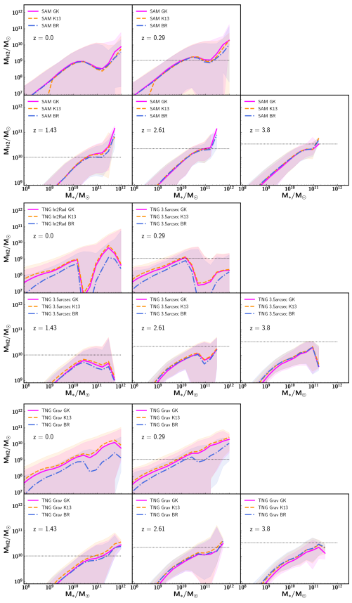
Figure 1: The H₂ mass of galaxies at different redshifts as a function of their stellar mass as predicted by the models. No galaxy selections were applied to the model galaxy population. The top two rows correspond to the SC SAM. The middle two rows depict IllustrisTNG when adopting the ‘3.5arcsec’ aperture ( note that at $z=0$ we use the ‘In2Rad’ aperture). The bottom two rows show IllustrisTNG when adopting the ‘Grav’ aperture. In all cases, we show results with the three H₂ partitioning recipes adopted in this work (GK: solid pink; K13: dashed orange; BR: dotted-dashed blue). The thick lines mark the median of the galaxy population, whereas the shaded regions mark the two-sigma scatter of the population. The dotted black horizontal line marks the sensitivity limit of ASPECS.

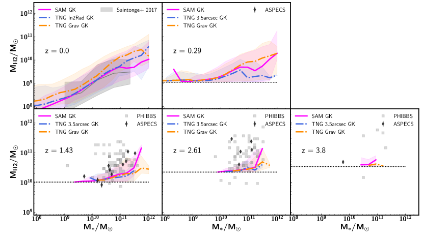
Figure 2: The predicted and observed H₂ mass of galaxies at different redshifts as a function of their stellar mass. For the theoretical data, we account for observational selection effects. The results from SC SAM (solid pink) and from IllustrisTNG are shown by adopting the GK H₂ partitioning recipe. We show predictions for IllustrisTNG when adopting the ‘3.5arcsec’ (dashed blue) and ‘Grav’ (dotted-dashed orange) apertures (at $z=0$, the ‘3.5arcsec’ aperture is replaced by the ‘In2Rad’ aperture). In this Figure we assume $\alpha_{\rm CO}=3.6\,\rm{M}_{\odot}/(\rm{K}\,\rm{km/s}\,\rm{pc}^{2})$. At $z=0$ a comparison is done to observational data from Saintonge et al. (2017). To allow for a fair comparison and remove the contribution by quiescent galaxies, a selection criterion of $\log{\rm{SFR}}>\log{\rm{SFR}_{\rm MS}}(\rm{M}_{*})-0.4$ is applied to both the observed and modeled galaxies at $z=0$, where $\log{\rm{SFR}_{\rm MS}}(\rm{M}_{*})$ marks the SFR of galaxies on the main sequence of star formation, following the definition of Speagle et al. (2014). At higher redshifts model predictions are compared to the detections of ASPECS, as well as the compilation of CO detected galaxies presented as a part of PHIBBS in Tacconi et al. (2018). At these redshifts the ASPECS selection function is applied to the model galaxies (and depicted by the dotted black horizontal line). The solid lines mark the median of the galaxy population, whereas the shaded regions mark the two-sigma scatter of the population. The different models are only partially able to reproduce the ASPECS and PHIBBS detections. We furthermore find that the ASPECS sensitivity sets a strong cut on the overall galaxy population (compare to Figure 1).

4 Results and comparison to observations

In this Section we compare the H₂ model predictions by the IllustrisTNG simulation and the SC SAM to the results of the ASPECS survey, by adopting a CO–to–H₂ conversion factor of $\alpha_{\rm CO}=3.6\,\rm{M}_{\odot}/(\rm{K}\,\rm{km/s}\,\rm{pc}^{2})$ for the observations following the ASPECS survey (we will change this assumption in our discussion in Section 5). Where appropriate, we also include additional datasets to allow for a broader comparison and to take into account observational sensitivity limits and field-to-field variance effects.

4.1 H₂ scaling relation

4.1.1 Inherent results

We present the H₂ mass of galaxies predicted from IllustrisTNG and the SC SAM as a function of their stellar mass at $z=0$ and the median redshifts of ASPECS in Figure 1. This figure includes all modeled galaxies at a redshift (i.e., no selection function is applied) and shows predictions for the H₂ mass based on all H₂ partitioning recipes considered in this work. We show the predictions for IllustrisTNG when adopting the ‘Grav’ aperture and the ‘3.5arcsec’ aperture (at $z=0$ replaced by the ‘In2Rad’ aperture). We depict for reference the sensitivity limit of ASPECS as a dotted horizontal line in all the panels corresponding to galaxies at $z>0$ (adopting the same CO excitation conditions and CO–to–H₂ conversion factor as ASPECS, $\alpha_{\rm CO}=3.6\,\rm{M}_{\odot}/(\rm{K}\,\rm{km/s}\,\rm{pc}^{2})$, and assume a CO line width of 200 km/s (a typical value for main-sequence galaxies at $z>1$; a narrower linewidth yields a lower mass limit, whereas a broader linewidth yields a higher mass limit, see Gonzales et al. 2019 and Figure 9 in Boogaard et al. 2019 for a detailed discussion on the effect of the CO line width on the recovering fraction of galaxies and the H₂ sensitivity limit), for a detailed explanation of these choices see Section 3 and Decarli et al., 2019).

Firstly, we find no significant difference in the predicted average H₂ mass of galaxies by the three different H₂ partitioning recipes coupled to the SC SAM. When coupled to IllustrisTNG the GK and K13 recipes yield almost identical results. This is in line with the broader findings by Diemer et al. 2018. The BR recipe predicts lower H₂ masses at $z<0.3$, but identical H₂ masses at higher redshifts. Given the minimal deviations in the medians between the different H₂ partitioning recipes, we will show from now on only predictions by the GK partitioning method in the main body of this paper. Model predictions obtained when adopting the other H₂ partitioning recipes are provided in Appendix B.

Importantly, we find the H₂ mass of galaxies to increase as a function of stellar mass for the SC SAM and IllustrisTNG when adopting the ‘Grav’ aperture, independent of redshift. At $z<3$ we see a decrease in the median H₂ mass for galaxies with a stellar mass larger than $10^{10}\,\rm{M}_{\odot}$. This decrease is stronger for the SC SAM than for IllustrisTNG with the ‘Grav’ aperture. This drop in the median represents the contribution from passive galaxies that host little molecular hydrogen, driven by the active galactic nucleus feedback mechanism. These galaxies have H₂ masses that are below the sensitivity limit of ASPECS. The upturn at the highest stellar masses corresponds to a low number of central galaxies that are still relatively gas rich.

When adopting the ‘3.5arcsec’ aperture for IllustrisTNG we see a different behaviour from the ‘Grav’ aperture. At $z=0.29$ and $z=1.43$ there is a much stronger drop in the median H₂ mass of galaxies at masses larger than $10^{10}\,\rm{M}_{\odot}$. This suggests that the bulk of the H₂ reservoir of the subhalos is outside of the aperture corresponding to the ASPECS beam at these redshifts. A beam with a diameter of 3.5 arcsec at $z=0.29$ corresponds to a size smaller than 2 times the stellar half-mass radius of the galaxies in IllustrisTNG with $M_{*}>10^{10}\,\rm{M}_{\odot}$ (Genel et al., 2018), suggesting that not all the molecular gas close to the stellar disk is captured. An AGN may furthermore move baryons to larger distances away from the center of the galaxies (outside of the aperture), but this has to be tested further by looking at the resolved H₂ properties of galaxies with IllustrisTNG. Stevens et al. (2018) find a similar drop at $z=0$ in the total cold gas mass (Hi plus H₂) of IllustrisTNG galaxies at similar stellar masses and also argue that an AGN feedback may be responsible for this.

Putting the predicted H₂ mass in contrast to the ASPECS sensitivity limit gives an idea of which galaxies might be missed by ASPECS. At $z=0.29$ the ASPECS sensitivity limit is below the median of the entire population of galaxies with stellar masses larger than $10^{10}\,{\rm M}_{\odot}$ for the SC SAM and IllustrisTNG when adopting the ‘Grav’ aperture. When adopting the ‘3.5arcsec’ aperture the situation changes, and only the most H₂ massive galaxies are picked up by the ASPECS survey (well above the median). The same conclusions are roughly true at $z=1.43$. At $z=2.61$ the ASPECS sensitivity limit is below the median of the galaxy population as predicted by the SAM for galaxies with $M_{*}>10^{11}\,\rm{M}_{\odot}$. The ASPECS survey is sensitive to the galaxies with the largest H₂ masses with stellar masses in the range $10^{10}\,\rm{M}_{\odot}<M_{*}<10^{11}\,\rm{M}_{\odot}$. Galaxies with lower stellar masses are excluded by the ASPECS sensitivity limit, according to the predictions by the SC SAM. The ASPECS sensitivity limit at $z=2.61$ is always above the median predictions from IllustrisTNG, independent of the aperture. At $z=3.8$ the ASPECS sensitivity limit is always above the median predictions by the models (both the SC SAM and IllustrisTNG). According to the models, ASPECS is only sensitive to galaxies with stellar masses $\sim 10^{11}\,\rm{M}_{\odot}$ with the most massive H₂ reservoirs (see Section 5 for a more in depth discussion on this).

4.1.2 Mocked results

In Figure 2 we again present the H₂ mass of galaxies as a function of their stellar mass at $z=0$ and at the median redshifts of ASPECS predicted from IllustrisTNG and the SC SAM. Differently from the previous Figure, we now take into account the selection functions that characterize the observational datasets we compare to. In particular, in this Figure, the predictions are compared to observed H₂ masses of galaxies from Saintonge et al. (2017) at $z=0$, and to the detections from the ASPECS surveys (all detections with a signal-to-noise ratio higher than 6.4). as well as a compilation presented in Tacconi et al. (2018) as a part of the PHIBBS (IRAM Plateau de Bure HIgh-z Blue Sequence Survey) survey at higher redshifts. At $z=0$ a selection criterion of $\log{\rm{SFR}}>\log{\rm{SFR}_{\rm MS}}(\rm{M}_{*})-0.4$ is applied to both the observed and modeled galaxies, where $\log{\rm{SFR}_{\rm MS}}(\rm{M}_{*})$ marks the SFR of galaxies on the main sequence of star-formation at $z=0$ following the definition of Speagle et al. (2014). At higher redshifts we only adopt the ASPECS CO sensitivity based selection criterion. ASPECS is sensitive to sources with an H₂ mass of $\sim 10^{9}\rm\rm{M}_{\odot}$ at $z=0.29$ and $\sim 10^{10},\,2\times 10^{10},\,$and $3\times 10^{10}\,\rm{M}_{\odot}$, at $z\approx 1.43,\,2.61$ and $3.8$, respectively (see Boogaard et al. 2019, Decarli et al. 2019, and Gonzales et al. 2019, for more details). PHIBBS selected galaxies based on a lower-limit in stellar mass and SFR. The galaxies in PHIBBS that have most massive H₂ reservoir also meet the ASPECS criterium.

At $z=0$ the predictions by the IllustrisTNG model are in general in good agreement with the observations (Diemer et al. 2019 presents a more detailed comparison of the H₂ mass properties of galaxies at $z=0$ between model predictions and observations, accounting for beam/aperture effects and different selection functions). The typical spread in the relation between H₂ mass and stellar mass is smaller for the model galaxies than the observed galaxies (it is worthwhile to note that the sample size of the observed galaxies is significantly smaller). At higher redshifts, on the other hand, a large fraction of the galaxies detected by ASPECS at $z\geq 1.43$ are not predicted by either IllustrisTNG (independent of the adopted aperture) or the SC SAM, i.e., the observed galaxies lie outside of the two-sigma scatter derived from the models. Similarly, a large fraction of the galaxies that are part of the PHIBBS data compilation also lie outside the two-sigma scatter on the predictions by the different models (also at $z\sim 3.8$). This suggests that the models predict H₂ reservoirs as a function of stellar mass that are not massive enough at $z\sim 1-3$.

Note that the median trends predicted from IllustrisTNG and the SC SAM at $z=0$ are essentially identical at low stellar masses, $\lesssim 10^{11}\,\rm{M}_{\odot}$. However, they diverge at larger stellar masses. The H₂ masses predicted from IllustrisTNG at $z=0$ are a factor $\sim 2$ higher than the SC SAM’s ones above $10^{11}\,\rm{M}_{\odot}$, the precise estimate depending on the adopted aperture. At $z\sim 0.29$ the H₂ scaling relations predicted by the models when accounting for the ASPECS sensitivity limits begin to differ for galaxies with stellar masses larger than $\sim 7\times 10^{10}\,\rm{M}_{\odot}$. At higher redshifts, the SC SAM and IllustrisTNG predict similar H₂ masses for galaxies with stellar masses less than $10^{11}\,\rm{M}_{\odot}$ (an artefact of the imposed selection limit), while at larger stellar masses the SAM predicts slightly more massive H₂ reservoirs at fixed stellar mass. Overall, the predictions of the SC SAM and IllustrisTNG are surprisingly similar, considering the large number of differences in the underlying modeling approach.

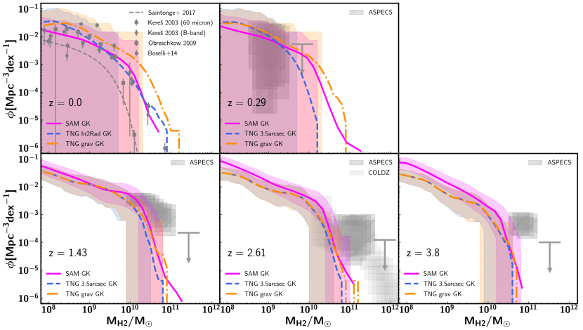
Figure 3: The predicted and observed H₂ mass function of galaxies assuming $\alpha_{\rm CO}=3.6\,\rm{M}_{\odot}/(\rm{K}\,\rm{km/s}\,\rm{pc}^{2})$ at $z=0$ and the redshifts probed by ASPECS. Model predictions are shown for the SC SAM (solid pink) and IllustrisTNG (‘3.5arcsec’ aperture: dashed blue; ‘Grav’ aperture: dashed-dotted orange), both models adopting the GK H₂ partitioning recipe. In this Figure the thick lines mark the mass function based on the entire simulated box ($\sim 100$ cMpc on a side for IllustrisTNG, $\sim 142$ cMpc on a side for the SC SAM). The colored shaded regions mark the two-sigma scatter when calculating the H₂ mass function in 1000 randomly selected cones that capture a volume corresponding to the volume probed by ASPECS at the given redshifts (Table 1). At $z=0$ the model predictions are compared to observations from Keres et al. (2003), Obreschkow & Rawlings (2009), Boselli et al. (2014), and Saintonge et al. (2017). At higher redshifts the model predictions are compared to observations from the ASPECS and COLDZ (Riechers et al., 2018) surveys.

4.2 The evolution of the H₂ mass function

We show the H₂ mass function of galaxies as predicted from IllustrisTNG and the SC SAM for the GK H₂ partitioning recipe in Figure 3 (the H₂ mass functions predicted using the other H₂ partitioning recipes are presented in Appendix B, where we show that they are very similar). The H₂ mass functions are shown at $z=0$ and at the median redshifts probed by ASPECS. The theoretical mass functions are derived by accounting for all the galaxies in the full simulation box ($\sim 100$ cMpc, solid line). The shaded regions mark the spread in the mass function when calculating it in smaller boxes representing the ASPECS volume, which is further discussed in Section 4.2.1. The mass functions at $z=0$ are compared to observations taken from from Keres et al. (2003), Obreschkow & Rawlings (2009), Boselli et al. (2014), and Saintonge et al. (2017, assuming a CO–to–H₂ conversion factor of $\alpha_{\rm CO}=3.6\,\rm{M}_{\odot}/(\rm{K}\,\rm{km/s}\,\rm{pc}^{2})$). The Obreschkow & Rawlings (2009) and Keres et al. (2003) mass functions are based on the same dataset, only Obreschkow & Rawlings (2009) assumes a variable CO–to–H₂ conversion factor as a function of metallicity (unlike ASPECS) instead of a fixed CO–to–H₂ conversion factor. At higher redshifts we compare the model predictions to the results from ASPECS, as well as the results from the COLDZ survey at $z\sim 2.6$ (Pavesi et al., 2018; Riechers et al., 2018).

The H₂ mass function at $z=0$ predicted by the SC SAM is in good agreement with the observations (Keres et al., 2003; Boselli et al., 2014; Saintonge et al., 2017). The mass function as predicted from IllustrisTNG when adopting the ‘In2Rad’ aperture (similar to the observed aperture) is also in rough agreement with the observations. When adopting the ‘Grav’ aperture the number densities of the most massive H₂ reservoir are instead too high. This difference highlights the importance of properly matching the aperture over which measurements are taken, especially at low redshifts and at the high mass end. Diemer et al. (2019) presents a robust comparison between model predictions from IllustrisTNG and observations at $z=0$, better accounting for the beam size of the various observations at $z=0$ than is done in this work.

Both the SC SAM and IllustrisTNG reproduce the the observed H₂ mass function by ASPECS at $z\sim 0.29$ (independent of the aperture). These are at masses below the knee of the mass function. Indeed, the volume probed by ASPECS at $z\sim 0.29$ is rather small, which explains the lack of galaxies detected with H₂ masses larger than a few times $10^{9}\,\rm{M}_{\odot}$. For the most massive H₂ reservoirs at $z=0.29$, on the other hand, the two models (and the choice of different apertures) return significantly different results: at fixed number density, the corresponding H₂ mass differs by a factor of five between the two IllustrisTNG apertures, with the SC SAM in between.

At $z>1$ the predictions for the H₂ number densities by the different models and their respective apertures are very close to each other. On average the SC SAM predicts number densities that are $\sim 0.2$ dex higher. At $z=1.43$ the models only just reproduce the observed H₂ mass function around masses of $10^{10}\,\rm{M}_{\odot}$, but predict too few galaxies with H₂ masses larger than $3\times 10^{10}\,\rm{M}_{\odot}$. The predicted H₂ number densities at $z=2.61$ are in good agreement with COLDZ and ASPECS in the mass range $10^{10}\rm{M}_{\odot}\leq M_{\rm H2}\leq 6\times 10^{10}\rm{M}_{\odot}$. The models do not reproduce ASPECS at higher masses and at higher redshifts, predicting number densities that are too low. We will further quantify how well the models reproduce the observed H₂ mass function when taking the surface area into account in the next subsection.

Table 1: The volume (in comoving Mpc) probed by ASPECS in different redshift ranges, after correcting for the primary beam sensitivty (see Decarli et al., 2019).

Redshift range	Volume (cMpc3)
$0.003\leq z\leq 0.369$	338
$1.006\leq z\leq 1.738$	8198
$2.008\leq z\leq 3.107$	14931
$3.011\leq z\leq 4.475$	18242

4.2.1 Field-to-field variance effects on the H₂ mass function

Since ASPECS only surveys a small area on the sky, field-to-field variance may bias the observed number densities of galaxies towards lower or higher values. In Figure 3 the thick lines represent the H₂ mass function that is derived when calculating the H₂ mass function based on the entire simulated volume ($\sim$ 100 cMpc for TNG100). The shaded areas around the thick lines in Figure 3 quantify the effects of cosmic variance on the H₂ mass function. The shaded regions mark the two-sigma scatter when calculating the H₂ mass function in 1000 randomly selected cones through the simulated volume that capture a volume corresponding to the actual volume probed by ASPECS at the given redshifts (Table 1).

At $z=0.29$ the small area probed by ASPECS can lead to large differences in the observed H₂ mass function. This ranges from number densities less than $10^{-6}\,\rm{Mpc}^{-3}\,\rm{dex}^{-1}$ at the lower end of the two-sigma scatter to a few times $10^{-2}\,\rm{Mpc}^{-3}\,\rm{dex}^{-1}$ at the upper end of the two-sigma scatter at any H₂ mass. The galaxies with the largest predicted H₂ reservoirs at $z=0.29$ ($M_{\rm H2}>10^{10}\,\rm{M}_{\odot}$) will typically be missed by a survey like ASPECS (do not fall in between the two-sigma scatter). This is indeed reflected by the lack of constraints on the number density of galaxies with H₂ masses more massive than $10^{10}\,\rm{M}_{\odot}$ by ASPECS.

The volume probed by ASPECS at redshifts $z>1$ is significantly larger (see Table 1), which indeed results in less scatter in the H₂ number densities of galaxies due to field-to-field variance. The two-sigma scatter in the power-law component of the mass function is 0.2–0.3 dex for IllustrisTNG and the SC SAM. The scatter quickly increases at H₂ masses beyond the knee of the mass functions, ranging from number densities less than $10^{-6}\,\rm{Mpc}^{-3}\,\rm{dex}^{-1}$ to number densities a few times higher than inferred based on the entire simulated boxes. The model galaxies that host the largest H₂ reservoirs in the full modeled boxes are typically not recovered when focusing on small volumes similar to the volume probed by ASPECS.

We can make a fairer comparison between the predictions by the theoretical models and ASPECS by accounting for the small volume probed by ASPECS. Figure 3 shows that at $z>1$ the observed number density of galaxies with $M_{\rm H2}>10^{11}\,\rm{M}_{\odot}$ is outside of the two-sigma scatter of the model predictions by both IllustrisTNG (for both apertures) and the SC SAM. The number densities of galaxies with lower H₂ masses are within the two-sigma scatter of both models. Summarizing, both IllustrisTNG and the SC SAM do not predict enough H₂ rich galaxies (with masses larger than $10^{11}\,\rm{M}_{\odot}$) in the redshift range $1.4\leq z\leq 3.8$. This is in line with our findings in Section 4.1 that both IllustrisTNG and the SC SAM predict H₂ masses within this redshift range that are typically too low for their stellar masses compared to the observations from ASPECS and PHIBBS.

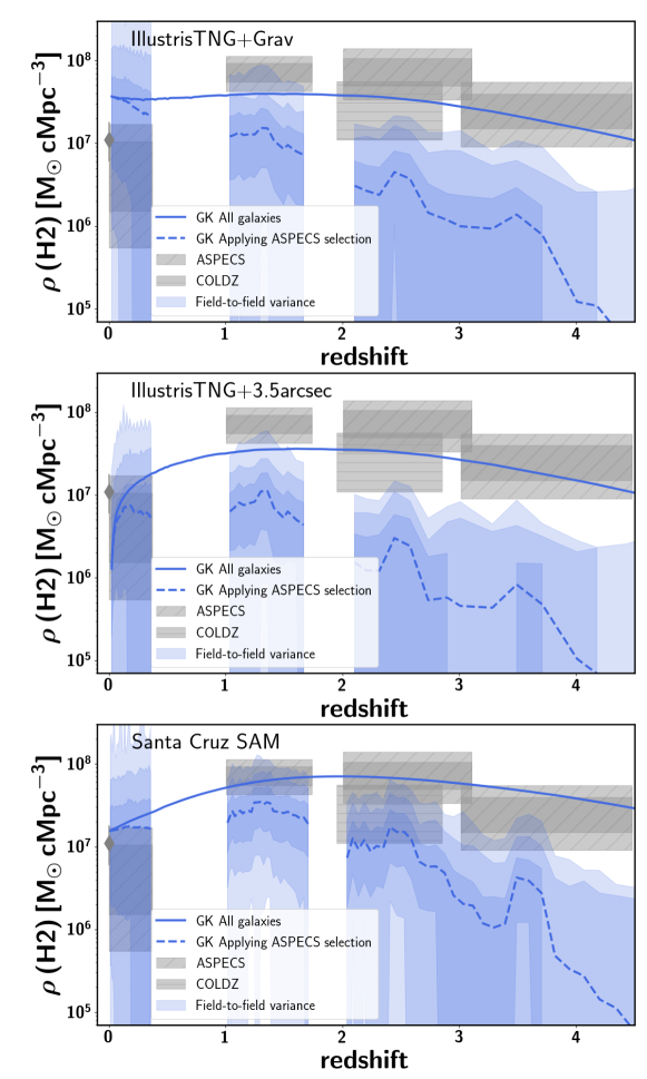
Figure 4: The predicted and observed H₂ cosmic density assuming $\alpha_{\rm CO}=3.6\,\rm{M}_{\odot}/(\rm{K}\,\rm{km/s}\,\rm{pc}^{2})$ as a function of redshift predicted from IllustrisTNG (‘Grav’ aperture, top; ‘3.5arcsec’ aperture, center), and the SC SAM (bottom), adopting the GK H₂ partitioning recipe. Solid lines correspond to the cosmic H₂ density based on all the galaxies in the entire simulated volume. Dashed lines correspond to the cosmic H₂ density when applying the ASPECS selection function. Shaded regions mark the 0th and 100th percentiles, two-sigma, and one-sigma scatter when calculating the H₂ cosmic density in 1000 randomly selected cones that capture a volume representing the ASPECS survey. Observations are from ASPECS (dark (light) grey mark the one (two) sigma uncertainty), COLDZ (Riechers et al., 2018), and from Saintonge et al. (2017) at $z=0$.

4.3 The H₂ cosmic density

We present the evolution of the cosmic density of H₂ within galaxies predicted by the SC SAM and IllustrisTNG when adopting the GK partitioning recipe in Figure 4 (predictions for the other partitioning recipes are presented in Appendix B). The solid lines correspond to the cosmic density derived based on all the galaxies in the entire simulated volume. The dashed lines correspond to a scenario where we only include galaxies with H₂ masses larger than the detection limit of ASPECS. The shaded region marks the H₂ cosmic density calculated in a box with a volume that corresponds to the volume probed by ASPECS at the appropriate redshift. This is further explained in Section 4.3.1. The model predictions are compared to $z=0$ observations taken from Keres et al. (2003) and Obreschkow & Rawlings (2009), as well as the observations from the ASPECS and COLDZ (Riechers et al., 2018) surveys at higher redshifts.

The H₂ cosmic density predicted from IllustrisTNG when adopting the ‘Grav’ aperture gradually increases till $z=1.5$ after which it stays roughly constant till $z=0$. At $z\sim$1, accounting for the ASPECS sensitivity limits can lead to a reduction in the H₂ cosmic density of a factor of three. The reduction is already one order of magnitude at $z\sim 2$ and further increases towards higher redshifts. The H₂ cosmic density predicted from IllustrisTNG when adopting the ‘3.5arcsec’ aperture increases till $z\sim 2$ and stays roughly constant till $z=1$. The H₂ cosmic density rapidly drops at $z<1$ by almost an order of magnitude till $z=0$. The difference between the low-redshift evolution predicted when adopting the ‘Grav’ aperture versus the ‘3.5arcsec’ aperture (especially at $z<0.5$) indicates that the ‘3.5arcsec’ aperture misses a significant fraction of the H₂ associated with the galaxy. The decrease in H₂ cosmic density when accounting for the ASPECS sensitivity limits is similar for the ‘3.5arcsec’ aperture as the ‘Grav’ aperture. The decrease is approximately a factor of three at $z=1$, approximately an order of magnitude at $z=2$, and this increases towards higher redshifts.

The H₂ cosmic density as predicted by the SC SAM when including all galaxies increases till $z\sim 2$, after which it gradually decreases by a factor of $\sim 4$ till $z=0$. Similar to IllustrisTNG, accounting for the ASPECS sensitivity limits results in a drop in the H₂ cosmic density of a factor of $\sim 3$ at $z=1$ and approximately an order of magnitude at $z>2$. On average, the SC SAM predicts H₂ cosmic densities at $z>1$ that are 1.5–2 times higher than predicted from IllustrisTNG (note that the SC SAM also predicts higher number densities for H₂-rich galaxies at these redshifts).

The difference between the total cosmic density (i.e., including the contribution from all galaxies in the simulated volume) and the H₂ cosmic density after applying the ASPECS sensitivity limit highlights the importance of properly accounting for selection effects when comparing model predictions to observations. Too often, comparisons are only carried out at face value ignoring these effects, creating a false impression. In this analysis we find that, when taking the ASPECS sensitivity limits into account, the cosmic densities predicted by the models are well below the observations at $z>1$, independent of the adopted model, H₂ partition recipe, and aperture. In the next subsection we will additionally take the effects of cosmic variance into account, in order to better quantify the (dis)agreement between ASPECS and the model predictions.

4.3.1 Field-to-field variance effects on the H₂ cosmic density

To understand the effects of field-to-field variance on the results from the ASPECS survey we also calculate the H₂ cosmic density in boxes representing the ASPECS volume. The shaded regions in Figure 4 mark the 0th and 100th percentiles, two-sigma, and one-sigma scatter when calculating the H₂ cosmic density in 1000 randomly selected cones through the simulated volume that correspond to the volume probed by ASPECS (also accounting for the ASPECS sensitivity limit).

At $z<0.3$ field-to-field variance can lead to large variations already (multiple orders of magnitude within the two-sigma scatter) in the derived H₂ cosmic density of the Universe, both for IllustrisTNG and the SC SAM. At higher redshifts the volume probed by ASPECS is larger and indeed the scatter in the H₂ cosmic density is smaller than at $z<0.3$.

The ASPECS observations at $z\sim 1.43$ are reproduced by a small fraction of the realizations predicted from IllustrisTNG (independent of the aperture), corresponding to the area above the two-sigma scatter (i.e., only up to 2.5% of the realizations drawn from IllustrisTNG reproduce the ASPECS observations). The observations at $z\sim 1.43$ are reproduced by a larger fraction of the realizations drawn from the SC SAM, covering the area between the one- and two-sigma scatter and above.

At $2<z<3$ all the realizations drawn from IllustrisTNG (independent of the chose aperture) predict H₂ cosmic densities lower than the ASPECS observations. At $z>3$ only a small fraction of the realizations reproduce the ASPECS observations when adopting the ‘Grav’ aperture, corresponding to the area between the two-sigma scatter and 100th percentile. The SC SAM predicts slightly higher cosmic densities on average, and indeed the ASPECS observations at $z>2$ fall within the two-sigma scatter of the realizations. Both IllustrisTNG and the SC SAM reproduce the observations taken from COLDZ in a subset of the realizations.

It is important to realize that a model is not necessarily ruled out if not all of the realizations agree with the ASPECS results. The fraction of realizations that agrees with the ASPECS results gives a feeling for the likelihood of a model being realistic. If only a small fraction (or none) of the realizations reproduces the ASPECS observations, this suggests that the model is very likely to be invalid (modulo the assumptions with regards to the interpretation of the observations). We will come back to this in the discussion.

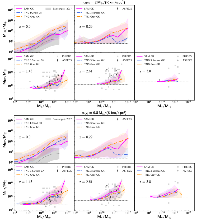
Figure 5: The predicted and observed H₂ mass of galaxies at different redshifts as a function of their stellar mass. The top five and bottom five panels correspond to a scenario where we adopt a CO–to–H₂ conversion factor of $\alpha_{\rm CO}=2.0\,\rm{M}_{\odot}/(\rm{K}\,\rm{km/s}\,\rm{pc}^{2})$ and $\alpha_{\rm CO}=0.8\,\rm{M}_{\odot}/(\rm{K}\,\rm{km/s}\,\rm{pc}^{2})$ for the observations and the simulations (through the ASPECS selection function), respectively. This Figure is otherwise identical to Figure 2.

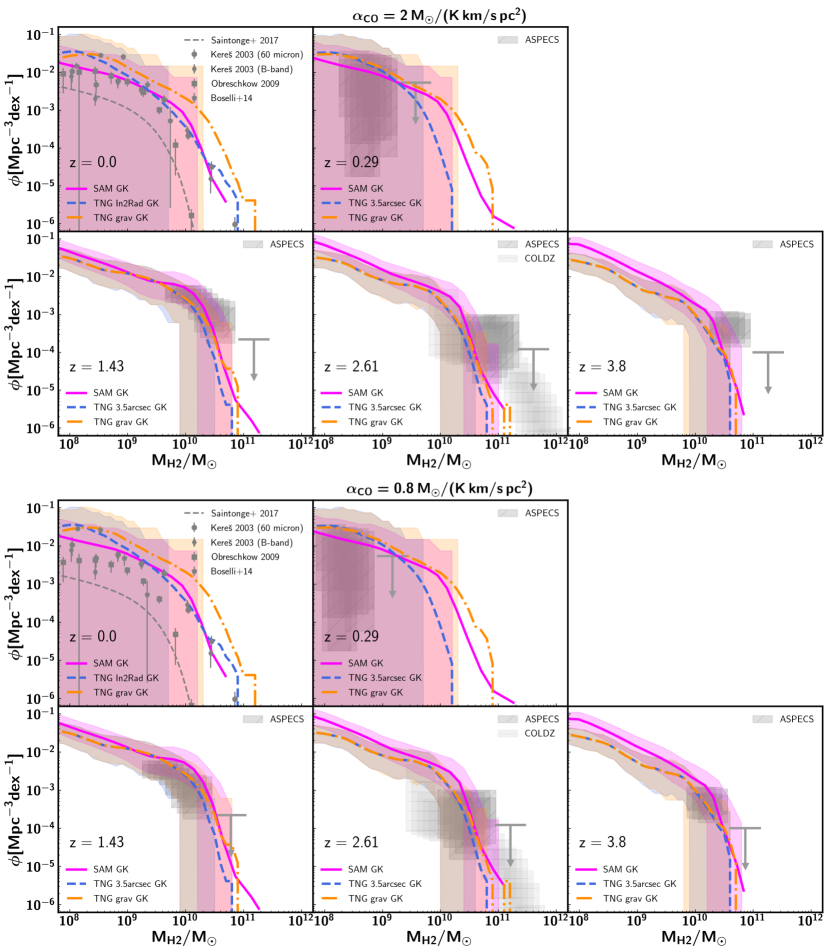
Figure 6: The predicted and observed H₂ mass function of galaxies at $z=0$ and the redshifts probed by ASPECS as predicted from IllustrisTNG and the SC SAM. The top five and bottom five panels correspond to a scenario where we adopt a CO–to–H₂ conversion factor of $\alpha_{\rm CO}=2.0\,\rm{M}_{\odot}/(\rm{K}\,\rm{km/s}\,\rm{pc}^{2})$ and $\alpha_{\rm CO}=0.8\,\rm{M}_{\odot}/(\rm{K}\,\rm{km/s}\,\rm{pc}^{2})$ for the observations, respectively. The data comparison is identical to Figure 3. In this Figure the thick lines mark the mass function based on the entire simulated box (100 Mpc on a side for IllustrisTNG, 142 Mpc on a side for the SC SAM). The shaded regions mark the two-sigma scatter when calculating the H₂ mass function in 1000 randomly selected cones that capture a volume corresponding to the volume probed by ASPECS at the given redshifts.

5 Discussion

5.1 Not enough H₂ in galaxy simulations?

One of the main results of this paper is that, when a CO–to–H₂ conversion factor $\alpha_{\rm CO}=3.6\,\rm{M}_{\odot}/(\rm{K}\,\rm{km/s}\,\rm{pc}^{2})$ is assumed, both IllustrisTNG and the SC SAM predict H₂ masses that are too low at a given stellar mass for galaxies at $z>1$ (Figure 2), do not predict enough H₂-rich galaxies (with H₂ masses larger than $3\times 10^{10}\,\rm{M}_{\odot}$; Figure 3), and predict cosmic densities that are only marginally compatible (SC SAM) or in tension (IllustrisTNG) with the ASPECS results after taking the ASPECS sensitivity limits into account (Figure 4). There are multiple choices that have to be made (both from the theoretical and observational side) that will affect this conclusion. In the remainder of this sub-section we discuss the main ones.

5.1.1 The strength of the UV radiation field impinging on molecular clouds

One of the theoretical challenges when calculating the H₂ content of galaxies is accounting for the impinging UV radiation field. Diemer et al. (2018) explored multiple approaches, by increasing and decreasing the UV radiation field when calculating the H₂ mass of cells in the IllustrisTNG simulation. The authors found differences in the predicted H₂ masses within a factor of 3 for the most extreme scenarios tested in their work (ranging from 1/10 to 10 times their fiducial UV radiation field, where a stronger UV radiation field results in lower H₂ masses), with differences away from their fiducial model up to a factor of 1.5-2. Although a systematic decrease in the UV radiation field could help to reproduce the cosmic density of H₂, it would go at the cost of reproducing the H₂ mass of galaxies and their mass function at $z=0$. Furthermore, a factor of 1.5–2 higher H₂ masses would still not be enough to overcome the tension between model predictions and observations at $z>2$. In the context of the SC SAM, SPT15 explored two different approaches to calculate the strength of the UV radiation field and found minimal changes in the predicted H₂ mass of galaxies with a $z=0$ halo mass larger than $10^{11}\,\rm{M}_{\odot}$.

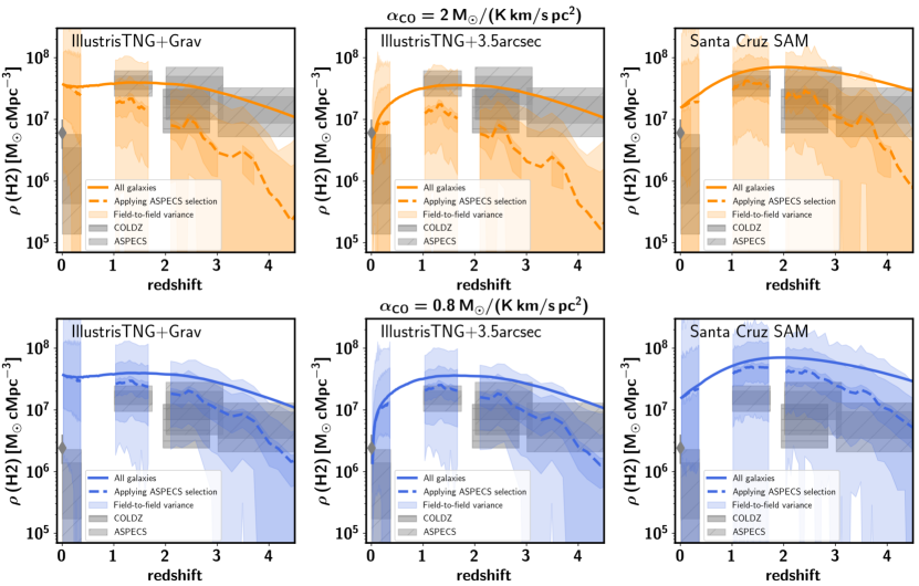
Figure 7: Model predictions for the H₂ cosmic density as a function of redshift as predicted from IllustrisTNG adopting the ‘Grav’ aperture (left), IllustrisTNG adopting the ‘3.5arcsec’ aperture (middle), and the SC SAM (right column), all of them adopting the GK H₂ partitioning recipe. The first and second rows correspond to a scenario where we adopt a CO–to–H₂ conversion factor of $\alpha_{\rm CO}=2.0\,\rm{M}_{\odot}/(\rm{K}\,\rm{km/s}\,\rm{pc}^{2})$ and $\alpha_{\rm CO}=0.8\,\rm{M}_{\odot}/(\rm{K}\,\rm{km/s}\,\rm{pc}^{2})$ for the observations, respectively. The solid lines corresponds to the cosmic H₂ density based on all the galaxies in the simulated volume, ignoring any selection function. The dashed lines correspond to the cosmic H₂ density in the entire box, applying the ASPECS selection function. The shaded regions mark the 0th and 100th percentiles, two-sigma, and one-sigma scatter when calculating the H₂ mass function in 1000 randomly selected cones that capture a volume corresponding to the volume probed by ASPECS at the given redshifts, also applying the ASPECS selection function. Model predictions are compared to the observational results from ASPECS (dark (light) gray mark the one (two) sigma uncertainty), as well as observations at $z=0$ from Keres et al. (2003) and Obreschkow & Rawlings (2009).

5.1.2 The CO–to–H₂ conversion factor and CO excitation conditions

One of the major observational uncertainties that could alleviate the tension between model predictions and the ASPECS results is the CO–to–H₂ conversion factor. The ASPECS survey adopts a conversion factor of $\alpha_{\rm CO}=3.6\,\rm{M}_{\odot}/(\rm{K}\,\rm{km/s}\,\rm{pc}^{2})$ for all CO detections. We first explore what values for the CO–to–H₂ conversion factor would be necessary to bring the model predictions into agreement with the observations. Changing the assumption for $\alpha_{\rm CO}$ has two immediate consequences. Firstly, it changes the value of the observed H₂ mass. Secondly, it changes the H₂ mass limit below which galaxies are not detected (since observations have a CO rather than an H₂ detection limit). Additionally it is important to better constrain the ratio between the CO J$=$1–0 and higher order rotational transitions of CO (J$=$2–1 to J$=$4–3 in the ASPECS survey). This ratio is currently assumed to be a fixed number, but has been shown to vary by a factor of a few from Milky Way type galaxies to ULIRGS.

We show the H₂ mass of galaxies as a function of stellar mass when varying the CO–to–H₂ conversion factor in Figure 5. The model predictions at $z=1.43$ are in significantly better agreement with the ASPECS detections when adopting $\alpha_{\rm CO}=2.0\,\rm{M}_{\odot}/(\rm{K}\,\rm{km/s}\,\rm{pc}^{2})$ than the standard value of $\alpha_{\rm CO}=3.6\,\rm{M}_{\odot}/(\rm{K}\,\rm{km/s}\,\rm{pc}^{2})$, although there are still a significant number of galaxies detected as part of the PHIBBS survey with H₂ masses outside of the two-sigma scatter of the models. More than half of the ASPECS detections at $z=2.61$ fall outside of the two-sigma scatter of the model predictions when adopting $\alpha_{\rm CO}=2.0\,\rm{M}_{\odot}/(\rm{K}\,\rm{km/s}\,\rm{pc}^{2})$. When assuming $\alpha_{\rm CO}=0.8\,\rm{M}_{\odot}/(\rm{K}\,\rm{km/s}\,\rm{pc}^{2})$, the model predictions are in good agreement with the ASPECS detections at $z=1.43$ and $z=2.61$ (although there are still a number of PHIBBS detections not reproduced by the models). We do note that the better match at $z>1$ comes at the cost of predicting H₂ masses that are too massive at $z=0$.

We present the observed and predicted H₂ mass function of galaxies when assuming different values for $\alpha_{\rm CO}$ in Figure 6. We find that when adopting $\alpha_{\rm CO}=2.0\,\rm{M}_{\odot}/(\rm{K}\,\rm{km/s}\,\rm{pc}^{2})$ the models reproduce the observed ASPECS H₂ mass function of galaxies over cosmic time (after accounting for cosmic variance, Figure 6 top panels vs. Figure 3). The number density of massive galaxies (larger than $10^{11}\,\rm{M}_{\odot}$) detected as a part of the COLDZ survey are still not reproduced by the models (i.e., the observed number densities are outside the two-sigma scatter of the model predictions). A CO–to–H₂ conversion factor of $\alpha_{\rm CO}=0.8\,\rm{M}_{\odot}/(\rm{K}\,\rm{km/s}\,\rm{pc}^{2})$ brings the model predictions for the H₂ mass functions from IllustrisTNG and the SC SAM into excellent agreement with the results from ASPECS at $1\lesssim z\lesssim 4$ (Figure 5, lower panels) and yields best agreement with the COLDZ results.

When adopting $\alpha_{\rm CO}=2.0\,\rm{M}_{\odot}/(\rm{K}\,\rm{km/s}\,\rm{pc}^{2})$, both models return a larger fraction of volume realizations that are consistent with the ASPECS and COLDZ H₂ cosmic densities at all redshifts (Figure 7, top panels). The ASPECS observations fall well within the two-sigma scatter of the predictions by the SC SAM. The observations fall in the area between the two-sigma scatter and 100th percentile of the predictions by IllustrisTNG when adopting an aperture corresponding to 3.5 arcsec. When adopting $\alpha_{\rm CO}=0.8\,\rm{M}_{\odot}/(\rm{K}\,\rm{km/s}\,\rm{pc}^{2})$, the ASPECS results match the predictions by both models (and both apertures for IllustrisTNG). For this scenario, only the lower 32% of all the realizations predicted by the SC SAM matches the observations. Similar conclusions hold when comparing the model predictions to the COLDZ survey. We do note that reproducing the ASPECS results at $z>1$ by varying the CO–to–H₂ conversion factor for all galaxies comes at the cost of predicting H₂ masses for galaxies at $z=0$ that are too massive.

Summarizing, the ASPECS survey would need to adopt a conversion factor of $\alpha_{\rm CO}\sim 0.8\,\rm{M}_{\odot}/(\rm{K}\,\rm{km/s}\,\rm{pc}^{2})$ for all observed galaxies at $z>0$ for the models to better reproduce the observed H₂ mass function and the H₂ cosmic density. The CO–to–H₂ conversion factor adopted by ASPECS of $\alpha_{\rm CO}=3.6\,\rm{M}_{\odot}/(\rm{K}\,\rm{km/s}\,\rm{pc}^{2})$ is motivated for main-sequence galaxies based on dynamical masses (Daddi et al., 2010), CO line spectral energy distribution (SED) fitting (Daddi et al., 2015) and solar metallicity $z>1$ main-sequence galaxies (Genzel et al., 2012). Nevertheless, conversion factors of $\alpha_{\rm CO}\sim 2\,\rm{M}_{\odot}/(\rm{K}\,\rm{km/s}\,\rm{pc}^{2})$ have been found for main-sequence galaxies at $z=1-3$ (e.g., Genzel et al., 2012; Popping et al., 2017b), also justifying the use of this value. A ULIRG CO conversion factor of $\alpha_{\rm CO}\sim 0.8\,\rm{M}_{\odot}/(\rm{K}\,\rm{km/s}\,\rm{pc}^{2})$ seems unrealistic for the entire sample, although it is not ruled out that, for example, the CO brightest sources in the ASPECS survey have a CO–to–H₂ conversion factor close to a ULIRG value. In reality, the CO–to–H₂ conversion factor will likely depend on a combination of ISM conditions and the gas-phase metallicity (Narayanan et al., 2012; Renaud et al., 2018) and vary between galaxies.

The COLDZ survey directly targets that CO J$=$1–0 emission line. Therefore no assumptions have to be made on the CO excitation conditions. The two models predicted in this work are in somewhat better agreement with COLDZ than ASPECS, although the models do not reproduce the H₂ massive galaxies found as a part of COLDZ either. The tension between the presented models and the observations can therefore not be fully accounted for by CO excitation conditions.

What this ultimately demonstrates is that there appears to be tension between the ASPECS survey results and model predictions, but a better quantification of this tension requires a better knowledge of the CO–to–H₂ conversion factor and a comparison between theory and observations by looking at CO directly. Zoom-simulations have suggested that $\alpha_{\rm CO}$ varies as a function of metallicity and gas surface density (Narayanan et al., 2012). Such variations will have an influence on the slope of the H₂ mass–stellar mass relation and the H₂ mass function, possibly further reducing the presented tension between observations and simulation. A number of cosmological semi-analytic models of galaxy formation have been coupled to carbon chemistry and radiative transfer codes in order to provide direct predictions for the CO luminosity of individual galaxies in cosmological volumes (Lagos et al., 2012; Popping et al., 2016, 2019). This approach bypasses the use of a CO–to–H₂ conversion factor to convert the observed quantities into H₂ masses. In line with our conclusions on the H₂ mass function, these models fail to reproduce the number of CO-bright sources detected by the ASPECS survey (Decarli et al., 2016, 2019).

5.2 Field-to-field variance and selection effects for ASPECS

Although ASPECS is providing a completely new view on the budget of gas available for star formation in the Universe, the conclusions from this survey are limited by the achievable survey design. The ASPECS survey only probes an area of 4.6 arcmin² on the sky. Although the survey marks the deepest effort of this kind so far, it is by far not large enough to overcome significant uncertainties due to field-to-field variance. Simulations are ideally suited to address how big the uncertainty in the derived conclusions is due to field-to-field variance.

In Section 4.2.1 we showed that the H₂ mass number densities derived for galaxies at $z>1$ when accounting for the volume of the ASPECS survey typically vary within a factor of two from the mass function derived for the entire simulated box. If we try to translate this to ASPECS, the ‘real’ H₂ mass function of the Universe might have number densities a factor of two lower/higher than measured as part of ASPECS. This number actually increases as a function of H₂ mass (because more massive galaxies are more strongly clustered), leading to possibly larger discrepancies for galaxies with H₂ masses of the order $10^{11}\,\rm{M}_{\odot}$.

A similar conclusion holds for the cosmic density of molecular hydrogen (see Section 4.3.1). Independent of the underlying model, the one-sigma scatter in the H₂ cosmic density at $z>1$ when applying the ASPECS sensitivity limits is typically within a factor of three from the cosmic density derived over the entire simulated volume (the two-sigma scatter is significantly larger). This number increases to a factor of 5 at the highest redshifts probed by ASPECS. At face value this means that the real cosmic density of H₂ may be up to a factor of three lower/higher than suggested by the observations so far. It is good to keep in mind that given that the models do not perfectly match the observed H₂ masses, our field-to-field variance statements may be incorrect as well. For reference, when no selection on H₂ is applied to the models, the typical one-sigma field-to-field variance-driven uncertainty is approximately 50% at $z>1$ for IllustrisTNG and the SC SAM.

It is hard to further quantify if the ‘real’ H₂ cosmic density (modulo the ASPECS CO selection function) is indeed a factor of 3–5 lower/higher than currently observed without any additional knowledge of the UDF. Spectroscopic observations of the UDF have suggested that the UDF is over-dense at $z\sim 0.67,\,0.73,\,1.1,\,\rm{and}\,1.61$ (Vanzella et al., 2005). Bouwens et al. (2007) find that the UDF is slightly under-dense at redshifts 3–5 (up to a factor of 1.5). Additional observations surveying a larger area on the sky at different locations will be necessary to properly bracket the expected variations in the H₂ cosmic density by field-to-field variance. Tests with the two simulations discussed in this work have shown that an increase in the covered area by an order of magnitude (ideally by looking at different regions on the sky) brings down the field-to-field variance driven uncertainty in the H₂ cosmic density to a factor of two at the two-sigma level and 30% at the one-sigma level.

In Section 4.3 we showed that, at least according to the models discussed in this work, a significant fraction of the cosmic H₂ budget is missed by the ASPECS survey. At $z=1$ this is a factor of three, whereas at $z>2$ this already corresponds to 90% or even more. Based on a study of the CO luminosity function, Decarli et al. (2019) estimate that the ASPECS survey accounts for approximately 80 % of the total CO luminosity emitted by galaxies. This is in stark contrast with model predictions, but fits with the idea that the models predict H₂ masses that are too low (and therefore less of the total H₂ density is picked up by ASPECS, or different CO–to–H₂ conversion factors and/or excitation conditions need to be applied). On top of this, the low-mass slope of the H₂ mass function at $z>2$ as predicted by the models in this paper is steeper than the slope assumed in Decarli et al. (2019, who adopt the same slope as ) for the CO luminosity function.

5.3 A comparison to earlier works

The finding that theoretical models do not predict enough H₂ in galaxies when adopting $\alpha_{\rm CO}=3.6\,\rm{M}_{\odot}/(\rm{K}\,\rm{km/s}\,\rm{pc}^{2})$ is not new. Popping et al. (2015a, b) reached the same conclusion for the SC SAM. The biggest difference to the work presented in this paper is that the authors compared the SC SAM predictions to inferred H₂ masses (and a sub-set of the PHIBBS galaxies also shown in this work), which come with their own uncertainties based on the underlying model and can lead to false conclusions.

Decarli et al. (2016, 2019) found a disagreement between the observed and modeled CO luminosity functions (a proxy for the H₂ mass function) at different redshifts, comparing the ASPECS CO luminosity functions to predictions from Lagos et al. (2012) and the SC SAM (Popping et al., 2016). The authors found that the models do not predict enough CO bright galaxies at $1\leq z\leq 3$. In the current work we presented a more robust comparison, taking field-to-field variance effects into account to better quantify the disagreement in the number of H₂-massive (CO-bright) galaxies. Furthermore, the uncertainty in the observed H₂ mass function and cosmic density used in the current work are tighter than in Decarli et al. (2016).

Decarli et al. (2016) also presented a comparison between the H₂ cosmic density as derived from the ASPECS pilot survey and predictions by three semi-analytic models (Obreschkow & Rawlings, 2009; Lagos et al., 2011; Popping et al., 2014b). Decarli et al. (2016) showed that these SAMs are able to reproduce the H₂ cosmic density up to $z=4$. The semi-analytic model presented in Xie et al. (2017) reproduces the H₂ cosmic densities from Decarli et al. (2016) from $z=0$–$4$. Lagos et al. (2018) predicts H₂ cosmic densities in agreement with the Decarli et al. (2016) results for galaxies at $z<1$ and $z>3$, but below the Decarli et al. (2016) results at redshifts $1\leq z\leq 3$. These predictions by SAMs seem very encouraging, but the comparisons were incorrect as the model predictions did not account for the ASPECS sensitivity limits. We have shown in Section 4.3 that accounting for the ASPECS sensitivity limits can lead to a reduction of a factor of up to 10 in the H₂ cosmic density (depending on the considered model and redshift).

Lagos et al. (2015) presented predictions for the cosmic density of H₂ based on the EAGLE (Schaye et al., 2015) simulations. The H₂ cosmic density predicted by Lagos et al. (2015) is only barely in agreement with the available results at that time from Walter et al. (2014). Lagos et al. (2015) do not directly account for the sensitivity limits of the Walter et al. (2014) observations, but do present the H₂ cosmic density when only considering galaxies with H₂ masses larger than $10^{9}\,\rm{M}_{\odot}$. This reduced their cosmic H₂ density by approximately 0.2 dex at $z<3$, and even more at higher redshifts, up to an order of magnitude at $z=4$. Applying the ASPECS sensitivity limits to the Lagos et al. (2015) model would further lower the predicted H₂ cosmic density. Lagos et al. (2015) furthermore does not reproduce the observed H₂ mass function from Walter et al. (2014) and predicts molecular hydrogen fractions lower than suggested by Tacconi et al. (2013) and Saintonge et al. (2013, although using different selection criteria than the samples presented in these works).

Davé et al. (2017) provide predictions for the H₂ cosmic density based on the MUFASA simulation (Davé et al., 2016). Davé et al. (2017) find a peak in their H₂ cosmic density at $z\sim 3$ after which the cosmic density decreases by a factor of three. The predicted densities based on all the galaxies in their simulated volume (not accounting for any sensitivity limit) are also significantly lower than the ASPECS results.

Putting all of these works together we can draw multiple conclusions. First of all, the added value of this paper is that it presents the most detailed comparison between model predictions and observations on this topic to date. On the one hand because it is based on the deepest CO survey to date, on the other hand because it accounts for sensitivity limits, field-to-field variance effects, and brackets systematic theoretical uncertainties (two different galaxy formation model approaches and different approaches for the partitioning of H₂). Second, a large number of galaxy formation models based on different methods (hydrodynamic and semi-analytic models) predict H₂ cosmic densities, H₂ masses, and H₂ mass functions that are too low compared to the observations. A better quantification of the latter will require constraining the CO–to–H₂ conversion factor in galaxies. Alternatively, a more precise comparison will require direct predictions of the CO luminosity of galaxies by galaxy formation models.

5.4 Putting the lack of H₂ in a broader picture

In this sub-section we aim to put the apparent lack of H₂ (the fuel for SF) in a broader picture by qualitatively discussing how predictions for the SFR of galaxies by different models agree with observations. A fair comparison would account for the different SF tracers used in the observations (and the average time scales over which they trace SF) as well as survey depth and survey area. Such a comparison should simultaneously also take into account the differences between the galaxies that ASPECS is sensitive to versus surveys focusing on other galaxy properties. Such a comparison should furthermore take into account that the spatial apertures and the time-scales a SFR tracer is sensitive to (e.g, up to $\sim$ 0.1 Gyr for UV based tracers) may be different from the spatial extent and instantaneous nature of a CO detection. Such a detailed comparison is beyond the scope of this work, we therefore limit ourselves to a brief qualitative discussion of SFR predictions in the literature where these effects were not taken into account. For example, many theoretical SFRs listed in the literature often represent the instantaneous SFR of gas taken directly from simulations.

The notion that galaxy formation models predict galaxies with H₂ masses that are too low at $z>1$ for their stellar mass is consistent with a broader picture of challenges for galaxy formation and evolution theory. For example, Somerville & Davé (2015) compared the predicted SFR of galaxies as a function of their stellar mass at $z>1$ for a wide range of galaxy formation models (including SAMs and hydrodynamical models) to observed SFRs. All the models considered in this compilation predict SFRs a factor of 2–3 lower than suggested by the majority of observations at $z=1-3$, while exhibiting better agreement at lower redshifts. The same conclusion holds for IllustrisTNG (see detailed discussions in Donnari et al. 2018). If the H₂ masses of modelled galaxies are too low for their stellar mass, it is not surprising that the SFRs of these galaxies are also too low when a molecular hydrogen based SF recipe is adopted. This is not necessarily true for models that adopt a total-cold gas based SFR recipe. However, the lack of H₂ suggests that there is either not enough gas or this gas is not dense enough to become molecular. A logical consequence is that this also leads to SFRs that are too low.

Since the H₂ cosmic densities predicted from IllustrisTNG and the SC SAM when assuming $\alpha_{\rm CO}=3.6\,\rm{M}_{\odot}/(\rm{K}\,\rm{km/s}\,\rm{pc}^{2})$ are in tension with the ASPECS observations, one would naively expect that the cosmic SFR density (cSFR, the SFR density of the universe) predicted from the models discussed in this work is also too low compared to the observations (if the SFR represent an instantaneous conversion from H₂ (gas) into stars). In Pillepich et al. (2018a), an “at face-value” comparison between the cosmic SFR predicted from IllustrisTNG and the data compilation presented in Behroozi et al. (2013a) reveals a factor $\sim$2 discrepancy at redshifts $1\leq z\leq 3$ (note however that Pillepich et al. did not attempt to apply any observational mock post processing to simulated galaxies or take other survey specifics into account). SPT15 reproduces the data compilation in Behroozi et al. (2013a) well in the redshift range $1\leq z\leq 3$. Yung et al. (2018) compares the cSFR predicted from the SC SAM to higher redshift observations and finds good agreement with the observational compilation (Yung et al. 2018 does include a UV luminosity sensitivity limit when calculating the cSFR to allow for a fair comparison to the observed cSFR). It is possibly surprising that the marginal agreement in the H₂ cosmic density predicted by the SC SAM does not result in a cSFR that is too low at $1\leq z\leq 3$, especially since the SFR of galaxies as a function of stellar mass is not reproduced. We again emphasize that in this redshift range observational selections were not taken into account in the comparison of the cSFR. A closer look at the results presented in SPT15 shows that the SC SAM predicts too many galaxies with a stellar mass below the knee of the stellar mass function at $1\leq z\leq 3$. The contribution of these galaxies to the total cSFR can (partially) explain the agreement between the predicted and observed cSFR, despite the disagreement in the H₂ cosmic density. This immediately demonstrates that a fair comparison taking selection functions and survey design into account is always important and necessary. It also demonstrates why integrated cosmic mass density is difficult to interpret – small changes in the abundance of low-mass objects can make a significant difference.

Davé et al. (2016) find that MUFASA predicts a total cSFR (not applying any selection functions and adopting the instantaneous SFR from the simulation) that is lower than the observed cSFR at redshifts $z=$1–3. Furlong et al. (2015) finds that the total cSFR predicted by EAGLE (again not accounting for selection effects and adopting the instantaneous SFR from the simulation) is systematically 0.2 dex below the observed cSFR at $z<3$. This suggests that also for these simulations the disagreement between observed and modeled cSFR can (at least partially) be explained by a lack of H₂ (star-forming) gas.

It is useful to keep in mind that even though the predicted star-forming main sequence and cSFR by different models appears to be in tension with observations, the same models find much better agreements with observational constraints on the galaxy stellar mass functions and the stellar mass density at the corresponding redshifts and masses (see e.g. Somerville et al. 2015 for the SC SAM, Furlong et al. 2015 for EAGLE, and Donnari et al. 2018 for IllustrisTNG, and discussions therein). This surprising mismatch could hint to issues in the comparisons (e.g. selection effects and different galaxy masses contributing to the different observables, and differently so at different cosmic times), problems of self-consistency in the observational data (Madau & Dickinson 2014 find that the intergral of the observed cSFR and the stellar mass density disagree by about a factor of two with each other, but see Driver et al. 2018), issues in the way star formation is modeled (e.g., Leja et al., 2018) and proceeds within simulated galaxies, or a combination of all.

Isolating the underlying physical mechanism that is responsible for the lack of massive H₂ reservoirs compared to the ASPECS survey is not straightforward. Within galaxy formation models, different physical processes acting on the baryons work in concert to shape galaxies. Changing the recipe for one of these processes with the aim of better reproducing a specific feature of galaxies can result in a mismatch for some other feature of galaxies. On top of that, different models often have different prescriptions for the physical processes acting on baryons in galaxies (even when they are similar in nature, the specifics may differ).

A number of models have attempted to alter their recipes for stellar feedback and the re-accretion of gas to better reproduce the SFR of galaxies at a given stellar mass over cosmic time (Henriques et al., 2015; White et al., 2015; Hirschmann et al., 2016). These efforts have demonstrated that changes to the re-accretion of ejected matter (Henriques et al., 2015; White et al., 2015) or a strongly decreasing efficiency of stellar feedback (Hirschmann et al., 2016, see also the implementation in Pillepich et al. 2018a) are promising, but not sufficient to solve the SFR discrepancy. We argue that besides the stellar mass and SFR of galaxies, a successful model will additionally have to address the lack of H₂ discussed in this paper. Hirschmann et al. (2016) and White et al. (2015) indeed showed that a delayed re-accretion and decreasing efficiency of stellar feedback with time lead to better agreement with the inferred H₂ masses of $z>1$ galaxies available at that time. This makes these changes promising, but more systematic theoretical exploration is needed. Additional venues to (simultaneously) explore include changes in the star-formation recipes to allow for a wider range in star-formation efficiencies.

6 Summary & Conclusions

In this paper we have presented predictions from IllustrisTNG (specifically the TNG100 volume) and the SC SAM for the H₂ content of galaxies, the H₂ mass function, and the H₂ cosmic density over cosmic time. These predictions were compared to results from ASPECS and COLDZ, specifically focusing on two issues; 1) how well do the models reproduce the results from the ASPECS survey; 2) how do field-to-field variance and the ASPECS sensitivity limits affect the results of ASPECS? We summarize our main results below:

• When adopting the canonical CO–to–H₂ conversion factor of $\alpha_{\rm CO}=3.6\,\rm{M}_{\odot}/(\rm{K}\,\rm{km/s}\,\rm{pc}^{2})$, the typical H₂ masses of galaxies at $z>1$ as a function of their stellar mass predicted from IllustrisTNG and the SC SAM are lower than the observations by a factor of 2–3. A significant number of galaxies detected as a part of ASPECS fall outside of the two-sigma scatter of these models.

• IllustrisTNG and the SC SAM do not reproduce the number of H₂-rich galaxies observed by ASPECS at $z>1$ (not enough galaxies with H₂ masses larger than $\sim 3\times 10^{10}\,\rm{M}_{\odot}$).

• The predictions by the SC SAM and IllustrisTNG for the H₂ cosmic density only just agree with the ASPECS results after taking field-to-field variance effects into account. This suggests that the predicted cosmic densities are too low.

• After applying the ASPECS sensitivity limit, the H₂ cosmic density is a factor of three (an order of magnitude) lower at $z=1$ ($z>2$) than the H₂ cosmic density obtained when accounting for all simulated galaxies (independent of the model).

• Adopting a global CO–to–H₂ conversion factor in the range $\alpha_{\rm CO}=2.0-0.8\,\rm{M}_{\odot}/(\rm{K}\,\rm{km/s}\,\rm{pc}^{2})$ would alleviate much of the tension between model predictions by IllustrisTNG and the SC SAM and the ASPECS results (although a uniform value of $\alpha_{\rm CO}=0.8\leavevmode\nobreak\ \rm{M}_{\odot}/(\rm{K}\,\rm{km/s}\,\rm{pc}^{2})$ appears unlikely). Likewise, a global change in the CO excitation conditions could alleviate some of the tension between models predictions and observations.

• Because ASPECS has a small survey area, field-to-field variance can lead to variations of typically up to a factor of three in the derived number densities for the H₂ mass function and cosmic density. It is thus crucial that besides sensitivity limits, field-to-field variance effects are also taken into account when comparing model predictions to observations. According to the outcome of the models discussed in this work, increasing the survey area by an order of magnitude would reduce the typical two-sigma uncertainty in the H₂ cosmic density due to field-to-field variance to a factor of 2 (one-sigma uncertainty is $\sim 30$ per cent).

• The systematic uncertainty between different H₂ partitioning recipes for predictions of the H₂ mass of galaxies, the H₂ mass function, and the H₂ cosmic density of the Universe is minimal.

The result that IllustrisTNG and the SC SAM do not predict enough H₂-rich galaxies at $z>1$ when adopting $\alpha_{\rm CO}=3.6\,\rm{M}_{\odot}/(\rm{K}\,\rm{km/s}\,\rm{pc}^{2})$ seems to be applicable to a wide range of galaxy formation models available in the literature. This paper is the first to better quantify this by using the ASPECS data, the most sensitive spectral survey currently available with ALMA, and properly accounting for selection effects and survey area. The lack of H₂ in $z>1$ model galaxies is possibly linked to a broader set of problems in galaxy formation and evolution theory, for instance a lack of star-formation in galaxies at these redshifts, and any solution should focus on all of these simultaneously. We anticipate that additional surveys with ALMA and the JVLA, focusing on larger and different areas in the sky and less H₂-rich galaxies will have the potential to further quantify the apparent lack of H₂ in galaxy formation models, providing crucial additional constraints for our understanding of galaxy formation and evolution. These surveys should additionally address the conversion of an observed CO luminosity into an H₂ gas mass, while galaxy formation models should simultaneously focus on providing direct predictions for the CO luminosity of galaxies.

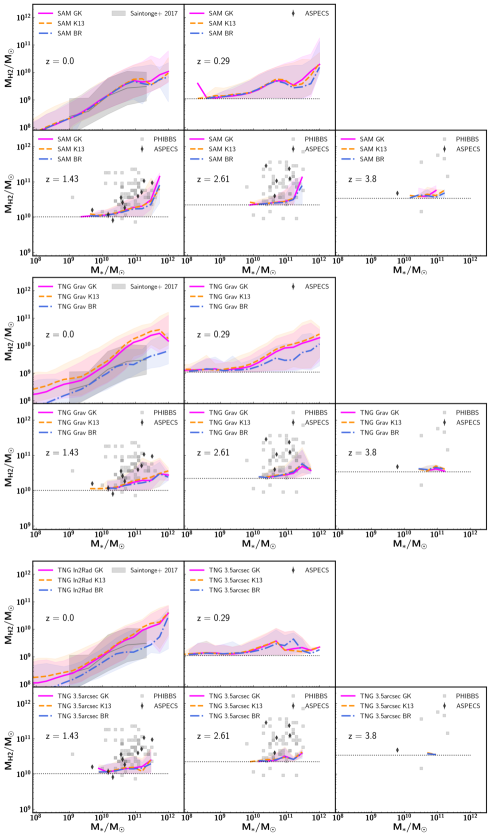
Figure 8: The H₂ mass of galaxies at different redshifts as a function of their stellar mass. Model predictions are shown for the SC SAM (top two rows), IllustrisTNG adopting the ‘3.5arcsec’ aperture (middle two rows, note that at $z=0$ this is replaced by then ‘In2Rad’ aperture) and IllustrisTNG when adopting the ‘Grav’ aperture (bottom two rows). For all models we show the GK (solid pink), the K13 (dashed orange), and the BR (dash-dotted blue) H₂ partitioning recipes. The selection function and data comparison is identical to Figure 2. The thick lines represent the median of the modeled galaxy population, whereas the shaded area represents the two-sigma scatter. At $z>0$ the H₂ masses predicted by the different model variants are almost identical. The models are not able to reproduce all ASPECS and PHIBBS detections.

Appendix A Additional molecular hydrogen fraction recipes

In Section 2.3 we presented the relevant equations for the GK H₂ partitioning recipe. In this Section of the appendix we describe in detail the remaining two H₂ partitioning recipes adopted in this work.

A.1 Blitz & Rosolowsky 2006 (BR)

The first recipe to calculate the molecular hydrogen fraction of the cold gas in each cell is based on the empirical pressure-based recipe presented by Blitz & Rosolowsky (2006, BR). They found a power-law relation between the disc mid-plane pressure and the ratio between molecular and atomic hydrogen, i.e.,

$$R_{\mathrm{H}_{2}}=\left(\frac{\Sigma_{\mathrm{H}_{2}}}{\Sigma_{\mathrm{HI}}}\right)=\left(\frac{P_{m}}{P_{0}}\right)^{\alpha_{\rm BR}}$$ (A1)

where $\Sigma_{\mathrm{H}_{2}}$ and $\Sigma_{\mathrm{HI}}$ are the H₂ and Hi surface densities, $P_{0}$ and $\alpha_{\rm BR}$ are free parameters that are obtained from a fit to the observational data, and $P_{m}$ is the mid-plane pressure acting on the galactic disc. We adopted $\log P_{0}/k_{\rm B}=4.23$ cm^-3 K and $\alpha_{\rm BR}=0.8$ from Leroy et al. (2008), where $k_{\rm B}$ is the Boltzmann constant.

When calculating the H₂ fraction of cells in IllustrisTNG following the BR approach we replace the mid-plane pressure $P_{m}$ by the thermal gas pressure of each cell, such that $P_{m}=P_{th}=u\rho(\gamma-1)$.

We follow the approach described in PST14 and SPT15 to calculate the H₂ fraction of gas in the SC SAM. The mid-plane pressure is calculated as Elmegreen (1989):

$$P_{\rm m}(r)=\frac{\pi}{2}\,G\,\Sigma_{\mathrm{gas}}(r)\left(\Sigma_{\mathrm{gas}}(r)+f_{\sigma}(r)\Sigma_{*}(r)\right)$$ (A2)

where G is the gravitational constant, $f_{\sigma}(r)$ is the ratio between $\sigma_{\mathrm{gas}}(r)$ and $\sigma_{*}(r)$, the gas and stellar vertical velocity dispersion, respectively. The stellar surface density profile $\Sigma_{*}(r)$ is modeled as an exponential with scale radius $r_{\mathrm{star}}$ and central density $\Sigma_{*,0}\equiv m_{*}/(2\pi r_{*}^{2})$, where $m_{*}$ is the stellar mass of a galaxy. Following Fu et al. (2012), we adopt $f_{\sigma}(r)=0.1\sqrt{\Sigma_{*,0}/\Sigma_{*}}$.

A.2 Krumholz 2013 (K13)

The second recipe is based on the work presented in Krumholz (2013) and builds upon the works presented in Krumholz et al. (2009a, b). Krumholz (2013) considers an ISM that is composed by a warm neutral medium (WNM) and a cold neutral medium (CNM) that are in pressure equilibrium. Krumholz (2013) finds that the equilibrium density of this two-phase medium should be three times the minimum density and writes

$$n_{\rm CNM,2p}=3n_{\rm CNM,min}=23G_{0}\frac{4.1}{1+3.1(Z/Z_{\odot})^{0.365}}\rm{cm}^{-3}.$$ (A3)

In the regime where the UV radiation field $G_{0}$ reaches zero, $n_{\rm CNM,2p}$ and the pressure also reach zero. This is an unphysical scenario and to account for this Krumholz (2013) defines a minimum CNM density to maintain hydrostatic balance, $n_{\rm CNM,hydro}$, based on the work by Ostriker et al. (2010). This density depends on the thermal pressure given as

$$P_{\rm th}=\frac{\pi G\Sigma^{2}_{\rm HI}}{4\alpha}\,\times\biggl{(}1+R_{\rm H2}+2\sqrt{(1+2R_{\rm H2})^{2}+\frac{32\xi_{d}\alpha f_{\rm w}c^{2}_{\rm w}\rho_{\rm sd}}{\pi G\Sigma^{2}_{\rm HI}}}\biggr{)},$$ (A4)

where $R_{\rm H2}=\Sigma_{\rm H2}/\Sigma_{\rm HI}$, $\alpha=5$ describes how much of the mid-plane pressure support is driven by turbulence, cosmic rays, and magnetic fields compared to the thermal pressure, $\xi_{d}=0.33$ is a geometrical factor, $c_{\rm w}=8\,\rm{km}\,\rm{s}^{-1}$ is the sound speed in the WNM, $f_{\rm w}=0.5$ the ratio between the thermal velocity dispersion and $c_{\rm w}$, and $\rho_{\rm sd}=0.01\rm{M}_{\odot}\,\rm{pc}^{-3}$ the stellar and dark matter density in the galactic disk. $n_{\rm CNM,hydro}$ furthermore depends on the maximum temperature of the CNM $T_{\rm CNM,max}=243\rm{K}$ (Wolfire et al., 2003), such that

$$n_{\rm CNM,hydro}=\frac{P_{\rm th}}{1.1\times k_{\rm B}T_{\rm CNM,max}}.$$ (A5)

The CNM density is then taken to be

$$n_{\rm CNM}=\rm{max}(n_{\rm CNM,2p},n_{\rm CNM,hydro}).$$ (A6)

Krumholz (2013) defines a dimensionless radiation field

$$\chi=7.2G_{0}\biggl{(}\frac{n_{\rm CNM}}{10\,\rm{cm}^{-3}}\biggr{)}^{-1}.$$ (A7)

The molecular hydrogen fraction is then given as

$$f_{H_{2}}=\begin{cases}1-0.75s/(1+0.25s)&s<2\\ 0&s\geq 2\end{cases}$$ (A8)

where

$$s=\frac{\ln(1+0.6\chi+0.01\chi^{2})}{0.6\tau_{c}}$$ (A9)

and

$$\tau_{c}=0.066f_{c}D_{\rm MW}\biggl{(}\frac{\Sigma_{\rm H}}{\rm{M}_{\odot}\,\rm{pc}^{-2}}\biggr{)}.$$ (A10)

$f_{c}$ marks a clumping factor that accounts for the scale over which the surface density is measured. The appropriate value for $f_{c}$ depends on the spatial scale over which the surface density is measured and is suggested to be $f_{c}=5$ on scales similar to the resolution of IllustrisTNG. The same clumping factor is adopted for the SC SAM. The molecular hydrogen fraction $f_{H_{2}}$ depends on the ratio between the molecular and atomic surface density $R_{\rm H2}$ and is solved iteratively.

Appendix B Predictions by different H₂ partitioning recipes

We present the predictions for the H₂ mass of galaxies, H₂ mass function, and H₂ cosmic density adopting the three different H₂ partitioning recipes in this Appendix. Figure 8 shows the H₂ mass as a function of stellar mass of galaxies after taking the ASPECS selection effects into account. These predictions are compared to the ASPECS results for the three different H₂ partitioning recipes adopted in this work, based on IllustrisTNG and the SC SAM, respectively. We find no difference in the predictions by the partitioning recipes for the SC SAM. When looking at IllustrisTNG we find that the BR partitioning recipe predicts H₂ masses that are systematically below the predictions by the other recipes at $z=0$ (0.1–0.2 dex). At higher redshifts the difference in the predictions by the three partitioning recipes is negligible.

Figure 9 shows the predictions from IllustrisTNG and the SC SAM for the H₂ mass function. When focusing on IllustrisTNG, the GK and K13 prescriptions result in almost identical H₂ mass functions at $z=0$. The Obreschkow & Rawlings (2009) observations are better reproduced when adopting the BR H₂ partitioning recipe. The BR prescription predicts number counts that are systematically below the predictions by the GK and K13 prescriptions, the difference increasing to $\sim 0.5$ dex at H₂ masses of $10^{10}\,\rm{M}_{\odot}$. At redshifts greater than zero the difference between the number densities predicted by the BR, GK, and K13 H₂ partitioning recipes decrease (at $z\sim 0.29$) or are minimal (at higher redshifts). Only in galaxies with H₂ masses less than $10^{9}\,\rm{M}_{\odot}$ at $z>3$ does the GK partitioning recipe predict number densities slightly less than the other two recipes. This mass range is not covered by the ASPECS survey.

When we focus on the SC SAM we see that at $z=0$ the BR prescription predicts slightly fewer galaxies with H₂ masses larger than $10^{10}\,\rm{M}_{\odot}$ than the other prescriptions. The same is true at $z=0.29$, whereas the predicted number densities are almost identical for the H₂ mass functions at higher redshifts.

We present the evolution of the H₂ cosmic density as predicted by IllustrisTNG and the SC SAM in Figure 10 for all three H₂ partitioning recipes considered in this work (GK pink, K13 orange, BR blue). We find some differences in the predictions of the H₂ cosmic density by the different H₂ partitioning recipes for IllustrisTNG, mostly in the evolution of the H₂ cosmic density at redshifts $z<3$. The H₂ cosmic density gradually increases till $z=3$ for the BR partitioning recipe after which it decreases by a factor of 4 till $z=0$. The GK and K13 partitioning recipes predict a gradual increase in the cosmic density till $z=2$, and a less pronounced decrease in the cosmic density till $z=0$ of only a factor of $\sim 2$ for the ‘Grav’ aperture. The predictions by the different partitioning recipes are similar when we account for the ASPECS sensitivity limits, typically within a factor of 1.5 and at $z>1$. The H₂ cosmic density evolution predicted by the SC SAM is almost identical for the three partitioning recipes. The cosmic densities predicted by the various partitioning recipes are also similar when accounting for the ASPECS selection function. This demonstrates that the systematic uncertainty between the different H₂ recipes is less than the typical uncertainty in the observations.

It is worthwhile to briefly focus on origin of the differences between the different H₂ partitioning recipes. We demonstrated that the different partitioning recipes yield almost identical predictions for the H₂ masses of galaxies as long as the underlying model is kept fixed. Only at $z=0$ does the BR partitioning recipe coupled to IllustrisTNG predict systematically lower H₂ masses. Diemer et al. (2018) also demonstrated that the systematic uncertainty on average mass scaling relations between different H₂ partitioning recipes coupled to IllustrisTNG is minimal (Diemer et al. 2018 came to this conclusion exploring an even larger sample of H₂ partitioning recipes). Krumholz & Gnedin (2011) demonstrated that the GK and Krumholz et al. (2009a) recipes result in almost identical H₂ fractions. This is to first order driven by the fact that both K13 and GK rely on the same set of input parameters, primarily the surface density of neutral hydrogen. Within the SC SAM, the BR recipe also primarily depends on the surface density of neutral gas, which explains the negligible differences in H₂ mass predictions by the different partitioning approaches. The BR recipe in the context of the IllustrisTNG model is the only one that does not primarily depend on the neutral gas surface density, but instead on the thermal pressure. Diemer et al. (2018) argues that this implementation of the BR partitioning recipe is incorrect, since the BR relation was calibrated based on observations of the Hi and H₂ gas surface density in local galaxies, rather than the thermal pressure as defined within simulations. Despite this, at $z>0$ the predictions between the different H₂ recipes for IllustrisTNG are nearly identical. It is furthermore curious that this approach yields possibly best agreement with the observational data at $z=0$ (although keep in mind that we did not properly mock the model predictions to include observational selection and aperture effects).

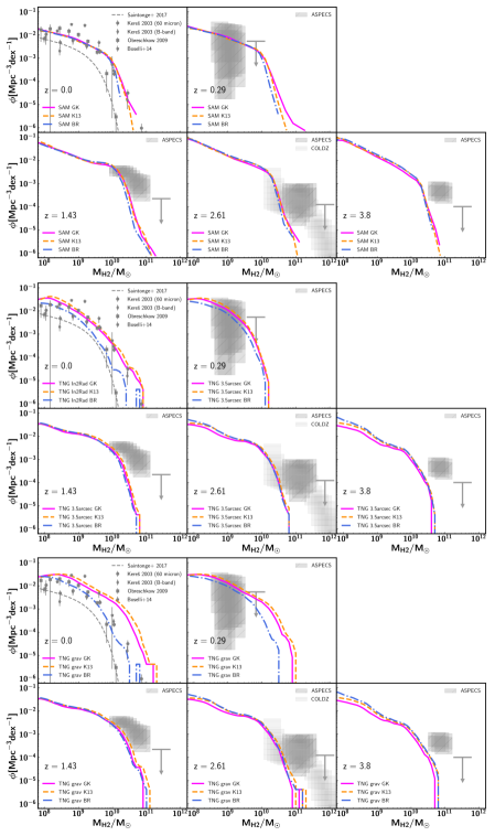
Figure 9: The H₂ mass function of galaxies at $z=0$ and the redshifts probed by ASPECS. Model predictions are shown for the SC SAM (top two rows), IllustrisTNG adopting the ‘3.5arcsec’ aperture (middle two rows, note that at $z=0$ this is replaced by then ‘In2Rad’ aperture) and IllustrisTNG when adopting the ‘Grav’ aperture (bottom two rows). For all models we show the GK (solid pink), the K13 (dashed orange), and the BR (dash-dotted blue) H₂ partitioning recipes. The data comparison is identical to Figure 3.

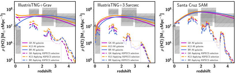
Figure 10: Model predictions for the H₂ cosmic density as a function of redshift as predicted from IllustrisTNG when adopting the ‘Grav’ aperture (left), IllustrisTNG when adopting the ‘3.5arcsec’ aperture (middle), and the SC SAM (right). We show the the GK (pink), K13 (orange), and BR (blue) H₂ partitioning recipes for all models. The solid lines correspond to the cosmic H₂ density in the entire box, ignoring any selection function. The dashed lines correspond to the cosmic H₂ density in the entire box, applying the ASPECS selection function. Model predictions are compared to the observations from ASPECS (dark (light) grey mark the one (two) sigma uncertainty), as well as observations at $z=0$ from Keres et al. (2003) and Obreschkow & Rawlings (2009).

References

- Aravena et al. (2016) Aravena, M., Decarli, R., Walter, F., et al. 2016, ApJ, 833, 68
- Bacon et al. (2017) Bacon, R., Conseil, S., Mary, D., et al. 2017, A&A, 608, A1
- Behroozi et al. (2013a) Behroozi, P. S., Wechsler, R. H., & Conroy, C. 2013a, ApJ, 770, 57
- Behroozi et al. (2013b) Behroozi, P. S., Wechsler, R. H., & Wu, H.-Y. 2013b, ApJ, 762, 109
- Bigiel & Blitz (2012) Bigiel, F., & Blitz, L. 2012, ApJ, 756, 183
- Blitz & Rosolowsky (2004) Blitz, L., & Rosolowsky, E. 2004, ApJ, 612, L29
- Blitz & Rosolowsky (2006) —. 2006, ApJ, 650, 933
- Bonatto & Bica (2011) Bonatto, C., & Bica, E. 2011, MNRAS, 415, 2827
- Boogaard et al. (2019) Boogaard, L., Decarli, R., Gonzalez, J., et al. 2019, submitted
- Boselli et al. (2014) Boselli, A., Cortese, L., Boquien, M., et al. 2014, A&A, 564, A66
- Bouwens et al. (2007) Bouwens, R. J., Illingworth, G. D., Franx, M., & Ford, H. 2007, ApJ, 670, 928
- Brennan et al. (2015) Brennan, R., Pandya, V., Somerville, R. S., et al. 2015, MNRAS, 451, 2933
- Bromm & Larson (2004) Bromm, V., & Larson, R. B. 2004, ARA&A, 42, 79
- Carilli & Walter (2013) Carilli, C. L., & Walter, F. 2013, ARA&A, 51, 105
- Chabrier (2003) Chabrier, G. 2003, PASP, 115, 763
- Christensen et al. (2012) Christensen, C., Quinn, T., Governato, F., et al. 2012, MNRAS, 425, 3058
- Daddi et al. (2010) Daddi, E., Bournaud, F., Walter, F., et al. 2010, ApJ, 713, 686
- Daddi et al. (2015) Daddi, E., Dannerbauer, H., Liu, D., et al. 2015, A&A, 577, A46
- Davé et al. (2017) Davé, R., Rafieferantsoa, M. H., Thompson, R. J., & Hopkins, P. F. 2017, MNRAS, 467, 115
- Davé et al. (2016) Davé, R., Thompson, R., & Hopkins, P. F. 2016, MNRAS, 462, 3265
- Decarli et al. (2014) Decarli, R., Walter, F., Carilli, C., et al. 2014, ApJ, 782, 78
- Decarli et al. (2016) Decarli, R., Walter, F., Aravena, M., et al. 2016, ApJ, 833, 69
- Decarli et al. (2019) —. 2019, submitted
- Diemer et al. (2018) Diemer, B., Stevens, A. R. H., Forbes, J. C., et al. 2018, ApJS, 238, 33
- Diemer et al. (2019) Diemer, B., Stevens, A. R. H., Lagos, C. d. P., et al. 2019, arXiv e-prints, arXiv:1902.10714
- Donnari et al. (2018) Donnari, M., Pillepich, A., Nelson, D., et al. 2018, arXiv e-prints, arXiv:1812.07584
- Driver et al. (2018) Driver, S. P., Andrews, S. K., da Cunha, E., et al. 2018, MNRAS, 475, 2891
- Dutton et al. (2010) Dutton, A. A., van den Bosch, F. C., & Dekel, A. 2010, MNRAS, 405, 1690
- Elmegreen (1989) Elmegreen, B. G. 1989, ApJ, 338, 178
- Faucher-Giguère et al. (2009) Faucher-Giguère, C.-A., Lidz, A., Zaldarriaga, M., & Hernquist, L. 2009, ApJ, 703, 1416
- Fu et al. (2010) Fu, J., Guo, Q., Kauffmann, G., & Krumholz, M. R. 2010, MNRAS, 409, 515
- Fu et al. (2012) Fu, J., Kauffmann, G., Li, C., & Guo, Q. 2012, MNRAS, 424, 2701
- Furlong et al. (2015) Furlong, M., Bower, R. G., Theuns, T., et al. 2015, MNRAS, 450, 4486
- Genel et al. (2014) Genel, S., Vogelsberger, M., Springel, V., et al. 2014, MNRAS, 445, 175
- Genel et al. (2018) Genel, S., Nelson, D., Pillepich, A., et al. 2018, MNRAS, 474, 3976
- Genzel et al. (2012) Genzel, R., Tacconi, L. J., Combes, F., et al. 2012, ApJ, 746, 69
- Gnedin (2012) Gnedin, N. Y. 2012, ApJ, 754, 113
- Gnedin & Kravtsov (2011) Gnedin, N. Y., & Kravtsov, A. V. 2011, ApJ, 728, 88
- Gonzales et al. (2019) Gonzales, J., Decarli, R., Walter, F., et al. 2019, submitted
- Haiman et al. (1996) Haiman, Z., Rees, M. J., & Loeb, A. 1996, ApJ, 467, 522
- Henriques et al. (2015) Henriques, B. M. B., White, S. D. M., Thomas, P. A., et al. 2015, MNRAS, 451, 2663
- Hirschmann et al. (2016) Hirschmann, M., De Lucia, G., & Fontanot, F. 2016, MNRAS, 461, 1760
- Hopkins (2004) Hopkins, A. M. 2004, ApJ, 615, 209
- Hopkins & Beacom (2006) Hopkins, A. M., & Beacom, J. F. 2006, ApJ, 651, 142
- Inami et al. (2017) Inami, H., Bacon, R., Brinchmann, J., et al. 2017, A&A, 608, A2
- Keres et al. (2003) Keres, D., Yun, M. S., & Young, J. S. 2003, ApJ, 582, 659
- Klypin et al. (2011) Klypin, A. A., Trujillo-Gomez, S., & Primack, J. 2011, ApJ, 740, 102
- Krumholz (2013) Krumholz, M. R. 2013, MNRAS, 436, 2747
- Krumholz et al. (2012) Krumholz, M. R., Dekel, A., & McKee, C. F. 2012, ApJ, 745, 69
- Krumholz & Gnedin (2011) Krumholz, M. R., & Gnedin, N. Y. 2011, ApJ, 729, 36
- Krumholz et al. (2008) Krumholz, M. R., McKee, C. F., & Tumlinson, J. 2008, ApJ, 689, 865
- Krumholz et al. (2009a) —. 2009a, ApJ, 693, 216
- Krumholz et al. (2009b) —. 2009b, ApJ, 699, 850
- Kuhlen et al. (2012) Kuhlen, M., Krumholz, M. R., Madau, P., Smith, B. D., & Wise, J. 2012, ApJ, 749, 36
- Lagos et al. (2011) Lagos, C. D. P., Baugh, C. M., Lacey, C. G., et al. 2011, MNRAS, 418, 1649
- Lagos et al. (2012) Lagos, C. d. P., Bayet, E., Baugh, C. M., et al. 2012, MNRAS, 426, 2142
- Lagos et al. (2018) Lagos, C. d. P., Tobar, R. J., Robotham, A. S. G., et al. 2018, MNRAS, 481, 3573
- Lagos et al. (2015) Lagos, C. d. P., Crain, R. A., Schaye, J., et al. 2015, MNRAS, 452, 3815
- Leja et al. (2018) Leja, J., Johnson, B. D., Conroy, C., et al. 2018, arXiv e-prints, arXiv:1812.05608
- Leroy et al. (2008) Leroy, A. K., Walter, F., Brinks, E., et al. 2008, AJ, 136, 2782
- Lilly et al. (1995) Lilly, S. J., Tresse, L., Hammer, F., Crampton, D., & Le Fevre, O. 1995, ApJ, 455, 108
- Madau & Dickinson (2014) Madau, P., & Dickinson, M. 2014, ARA&A, 52, 415
- Madau et al. (1996) Madau, P., Ferguson, H. C., Dickinson, M. E., et al. 1996, MNRAS, 283, 1388
- Marinacci et al. (2017) Marinacci, F., Grand, R. J. J., Pakmor, R., et al. 2017, MNRAS, 466, 3859
- Marinacci et al. (2018) Marinacci, F., Vogelsberger, M., Pakmor, R., et al. 2018, MNRAS, 480, 5113
- McKee & Krumholz (2010) McKee, C. F., & Krumholz, M. R. 2010, ApJ, 709, 308
- McKinnon et al. (2017) McKinnon, R., Torrey, P., Vogelsberger, M., Hayward, C. C., & Marinacci, F. 2017, MNRAS, 468, 1505
- Miller & Scalo (1979) Miller, G. E., & Scalo, J. M. 1979, ApJS, 41, 513
- Naiman et al. (2018) Naiman, J. P., Pillepich, A., Springel, V., et al. 2018, MNRAS, 477, 1206
- Narayanan et al. (2012) Narayanan, D., Krumholz, M. R., Ostriker, E. C., & Hernquist, L. 2012, MNRAS, 421, 3127
- Nelson et al. (2018a) Nelson, D., Pillepich, A., Springel, V., et al. 2018a, MNRAS, 475, 624
- Nelson et al. (2018b) Nelson, D., Kauffmann, G., Pillepich, A., et al. 2018b, MNRAS, 477, 450
- Obreschkow & Rawlings (2009) Obreschkow, D., & Rawlings, S. 2009, MNRAS, 394, 1857
- Ostriker et al. (2010) Ostriker, E. C., McKee, C. F., & Leroy, A. K. 2010, ApJ, 721, 975
- Pavesi et al. (2018) Pavesi, R., Sharon, C. E., Riechers, D. A., et al. 2018, ApJ, 864, 49
- Pillepich et al. (2018a) Pillepich, A., Springel, V., Nelson, D., et al. 2018a, MNRAS, 473, 4077
- Pillepich et al. (2018b) Pillepich, A., Nelson, D., Hernquist, L., et al. 2018b, MNRAS, 475, 648
- Planck Collaboration et al. (2016) Planck Collaboration, Ade, P. A. R., Aghanim, N., et al. 2016, A&A, 594, A13
- Popping et al. (2009) Popping, A., Davé, R., Braun, R., & Oppenheimer, B. D. 2009, A&A, 504, 15
- Popping et al. (2015a) Popping, G., Behroozi, P. S., & Peeples, M. S. 2015a, MNRAS, 449, 477
- Popping et al. (2019) Popping, G., Narayanan, D., Somerville, R. S., Faisst, A. L., & Krumholz, M. R. 2019, MNRAS, 482, 4906
- Popping et al. (2014a) Popping, G., Pérez-Beaupuits, J. P., Spaans, M., Trager, S. C., & Somerville, R. S. 2014a, MNRAS, 444, 1301
- Popping et al. (2017a) Popping, G., Somerville, R. S., & Galametz, M. 2017a, MNRAS, 471, 3152
- Popping et al. (2014b) Popping, G., Somerville, R. S., & Trager, S. C. 2014b, MNRAS, 442, 2398
- Popping et al. (2016) Popping, G., van Kampen, E., Decarli, R., et al. 2016, MNRAS, arXiv:1602.02761
- Popping et al. (2015b) Popping, G., Caputi, K. I., Trager, S. C., et al. 2015b, MNRAS, 454, 2258
- Popping et al. (2017b) Popping, G., Decarli, R., Man, A. W. S., et al. 2017b, A&A, 602, A11
- Porter et al. (2014) Porter, L. A., Somerville, R. S., Primack, J. R., & Johansson, P. H. 2014, MNRAS, 444, 942
- Rémy-Ruyer et al. (2014) Rémy-Ruyer, A., Madden, S. C., Galliano, F., et al. 2014, A&A, 563, A31
- Renaud et al. (2018) Renaud, F., Bournaud, F., Daddi, E., & Weiß, A. 2018, arXiv e-prints, arXiv:1811.06547
- Riechers et al. (2018) Riechers, D. A., Pavesi, R., Sharon, C. E., et al. 2018, ArXiv e-prints, arXiv:1808.04371
- Robertson & Kravtsov (2008) Robertson, B. E., & Kravtsov, A. V. 2008, ApJ, 680, 1083
- Rodríguez-Puebla et al. (2016) Rodríguez-Puebla, A., Behroozi, P., Primack, J., et al. 2016, MNRAS, 462, 893
- Saintonge et al. (2013) Saintonge, A., Lutz, D., Genzel, R., et al. 2013, ApJ, 778, 2
- Saintonge et al. (2017) Saintonge, A., Catinella, B., Tacconi, L. J., et al. 2017, ApJS, 233, 22
- Schaye et al. (2015) Schaye, J., Crain, R. A., Bower, R. G., et al. 2015, MNRAS, 446, 521
- Sijacki et al. (2015) Sijacki, D., Vogelsberger, M., Genel, S., et al. 2015, MNRAS, 452, 575
- Somerville & Davé (2015) Somerville, R. S., & Davé, R. 2015, ARA&A, 53, 51
- Somerville et al. (2012) Somerville, R. S., Gilmore, R. C., Primack, J. R., & Domínguez, A. 2012, MNRAS, 423, 1992
- Somerville et al. (2008) Somerville, R. S., Hopkins, P. F., Cox, T. J., Robertson, B. E., & Hernquist, L. 2008, MNRAS, 391, 481
- Somerville et al. (2015) Somerville, R. S., Popping, G., & Trager, S. C. 2015, MNRAS, 453, 4337
- Somerville & Primack (1999) Somerville, R. S., & Primack, J. R. 1999, MNRAS, 310, 1087
- Somerville et al. (2001) Somerville, R. S., Primack, J. R., & Faber, S. M. 2001, MNRAS, 320, 504
- Speagle et al. (2014) Speagle, J. S., Steinhardt, C. L., Capak, P. L., & Silverman, J. D. 2014, ApJS, 214, 15
- Springel (2010) Springel, V. 2010, MNRAS, 401, 791
- Springel & Hernquist (2003) Springel, V., & Hernquist, L. 2003, MNRAS, 339, 289
- Springel et al. (2018) Springel, V., Pakmor, R., Pillepich, A., et al. 2018, MNRAS, 475, 676
- Stevens et al. (2018) Stevens, A. R. H., Diemer, B., Lagos, C. d. P., et al. 2018, ArXiv e-prints, arXiv:1810.12158
- Tacconi et al. (2013) Tacconi, L. J., Neri, R., Genzel, R., et al. 2013, ApJ, 768, 74
- Tacconi et al. (2018) Tacconi, L. J., Genzel, R., Saintonge, A., et al. 2018, ApJ, 853, 179
- Thompson et al. (2014) Thompson, R., Nagamine, K., Jaacks, J., & Choi, J.-H. 2014, ApJ, 780, 145
- Torrey et al. (2014) Torrey, P., Vogelsberger, M., Genel, S., et al. 2014, MNRAS, 438, 1985
- Torrey et al. (2017) Torrey, P., Vogelsberger, M., Marinacci, F., et al. 2017, ArXiv e-prints, arXiv:1711.05261
- Trujillo-Gomez et al. (2011) Trujillo-Gomez, S., Klypin, A., Primack, J., & Romanowsky, A. J. 2011, ApJ, 742, 16
- Vanzella et al. (2005) Vanzella, E., Cristiani, S., Dickinson, M., et al. 2005, A&A, 434, 53
- Vogelsberger et al. (2013) Vogelsberger, M., Genel, S., Sijacki, D., et al. 2013, MNRAS, 436, 3031
- Vogelsberger et al. (2014a) Vogelsberger, M., Genel, S., Springel, V., et al. 2014a, Nature, 509, 177
- Vogelsberger et al. (2014b) —. 2014b, MNRAS, 444, 1518
- Vogelsberger et al. (2018) Vogelsberger, M., Marinacci, F., Torrey, P., et al. 2018, MNRAS, 474, 2073
- Walter et al. (2014) Walter, F., Decarli, R., Sargent, M., et al. 2014, ApJ, 782, 79
- Walter et al. (2016) Walter, F., Decarli, R., Aravena, M., et al. 2016, ApJ, 833, 67
- Weinberger et al. (2017) Weinberger, R., Springel, V., Hernquist, L., et al. 2017, MNRAS, 465, 3291
- White et al. (2015) White, C. E., Somerville, R. S., & Ferguson, H. C. 2015, ApJ, 799, 201
- Williams et al. (1996) Williams, R. E., Blacker, B., Dickinson, M., et al. 1996, AJ, 112, 1335
- Wolfire et al. (2003) Wolfire, M. G., McKee, C. F., Hollenbach, D., & Tielens, A. G. G. M. 2003, ApJ, 587, 278
- Xie et al. (2017) Xie, L., De Lucia, G., Hirschmann, M., Fontanot, F., & Zoldan, A. 2017, MNRAS, 469, 968
- Yung et al. (2018) Yung, L. Y. A., Somerville, R. S., Finkelstein, S. L., Popping, G., & Davé, R. 2018, ArXiv e-prints, arXiv:1803.09761