Tidal disruptions by rotating black holes: effects of spin and impact parameter
Abstract
We present the results of relativistic smoothed particle hydrodynamics simulations of tidal disruptions of stars by rotating supermassive black holes, for a wide range of impact parameters and black hole spins. For deep encounters, we find that: relativistic precession creates debris geometries impossible to obtain with the Newtonian equations; part of the fluid can be launched on plunging orbits, reducing the fallback rate and the mass of the resulting accretion disc; multiple squeezings and bounces at periapsis may generate distinctive X-ray signatures resulting from the associated shock breakout; disruptions can occur inside the marginally bound radius, if the angular momentum spread launches part of the debris on non-plunging orbits. Perhaps surprisingly, we also find relativistic effects important in partial disruptions, where the balance between self-gravity and tidal forces is so precarious that otherwise minor relativistic effects can have decisive consequences on the stellar fate. In between, where the star is fully disrupted but relativistic effects are mild, the difference resides in a gentler rise of the fallback rate, a later and smaller peak, and longer return times. However, relativistic precession always causes thicker debris streams, both in the bound part (speeding up circularization) and in the unbound part (accelerating and enhancing the production of separate transients). We discuss various properties of the disruption (compression at periapsis, shape and spread of the energy distribution) and potential observables (peak fallback rate, times of rise and decay, duration of super-Eddington fallback) as a function of the impact parameter and the black hole spin.
keywords:
black hole physics – hydrodynamics – relativistic processes – methods: numerical – galaxies: nuclei1 Introduction
As observational evidence for the tidal disruption of stars by supermassive black holes (SMBH) is mounting, the question remains how such observations can help determine black hole (BH) properties such as mass and spin (Mockler, Guillochon & Ramírez-Ruiz, 2019). While analytical calculations may be able to provide a strikingly accurate description of some features of such an event, including the famous decay of the fallback rate (Rees, 1988; Phinney, 1989), a relativistic tidal disruption event (TDE) is a highly non-linear outcome of the interplay between the stellar hydrodynamics and self-gravity, tidal accelerations from the black hole, radiation, potentially magnetic fields and – in extreme cases – nuclear reactions. To date, systematic numerical studies of relativistic TDEs are still lacking.
In this paper, we shall use the formalism introduced by Tejeda et al. (2017, henceforth TGRM+17), “relativistic hydrodynamics with Newtonian codes”, to perform an extensive study of canonical tidal disruption events around spinning black holes. The method combines an exact relativistic description of the hydrodynamical evolution of a fluid in Kerr spacetime with a quasi-Newtonian treatment of the fluid’s self-gravity. The only similar study of the parameter space we are aware of belongs to Guillochon & Ramírez-Ruiz (2013, henceforth GRR13), who analysed the dependency of Newtonian TDEs on the penetration factor , for two types of polytropes (with polytropic exponent and ), and with ranging from to (for ) and from to (for ).
High-resolution relativistic simulations of TDEs have only become feasible in recent years. Since the seminal paper by Laguna et al. (1993b), who tackled for the first time disruptions of Main-Sequence (MS) stars around Schwarzschild BHs, relatively few studies have continued the numerical investigation of relativistic TDEs: Kobayashi et al. (2004) repeated the simulations of Laguna et al. (1993b) (, and ) using essentially the same numerical method (Laguna, Miller & Zurek, 1993a), and additionally treated the disruption of a helium star with , with the goal of predicting the X-ray and gravitational wave signatures from such TDEs, while Bogdanović et al. (2004) used the same code to study a canonical disruption with and calculate the H emission-line luminosity of the resulting disc and debris tail. Cheng & Bogdanović (2014) presented three disruptions of MS stars with around SMBHs of masses , and , and of two of white dwarfs (WD) with , around a BH, focusing on the influence of relativistic effects on the fallback rate of the bound debris. Other authors have chosen to focus exclusively on the effect of General Relativity (GR) on WD disruptions by intermediate-mass black holes (IMBH), since they pose less of a computational challenge (Haas et al., 2012; Cheng & Evans, 2013; Shiokawa et al., 2015).
In recent years, another class of simulations, combining particle codes for the disruption part of a TDE and fixed metric general-relativistic Eulerian codes for the disc formation part, have improved our understanding of the process of accretion disc formation in TDEs (e.g., Sa̧dowski et al., 2016). However, these studies have generally focused on a very reduced set of initial parameters (one or two encounters being the norm), and have invariably approached TDEs on elliptical orbits in order to alleviate the tremendous scale problem of a typical parabolic encounter. These studies are complemented by pseudo-relativistic particle simulations of the disruption of stars on elliptical orbits, followed by the subsequent circularization (e.g., Bonnerot et al., 2016; Hayasaki, Stone & Loeb, 2013, 2016).
The literature of TDEs in Kerr spacetime is substantially sparser: aside from some older analytical and semi-analytical studies (Luminet & Marck, 1985; Frolov et al., 1994; Kesden, 2012), only two numerical studies have included the effects of the BH spin: a) Haas et al. (2012) presented six ultra-close TDEs of a WD by a Kerr IMBH with spin parameters and ; b) Evans, Laguna & Eracleous (2015) presented nine ultra-close TDEs of a solar-type star by a Kerr IMBH with spin parameters and . In both cases, the parameter range has been fine-tuned with the periapsis being close to the marginally bound radius of the BH, i.e., at the very limit of where a TDE could possibly take place.
All these studies necessarily focused on restrictive subsets of the parameter space (often chosen to reduce the otherwise prohibitive computational burden), and while they have answered important specific questions about the impact of GR on the disruption process and in particular on the circularization, they cannot provide an overview of Kerr TDEs across the range of impact parameters and spins. To date, this has only been achieved by (semi-)analytical means, by Kesden (2012).
To our knowledge, this paper is the first systematic numerical study of TDEs with relativistic hydrodynamics around Kerr BHs. Our goal is to analyse the disruption process from the initial approach until the second periapsis passage, and to: a) compare our findings with previous results (both for Newtonian and Kerr BHs) and with standard expectations based on theoretical arguments; b) determine the effects of GR in general, and of the BH spin in particular, on the various stages of the disruption; c) present a unified picture of tidal disruptions in Kerr spacetime (since we also treat the particular case , we implicitly include Schwarzschild BHs in our analysis).
2 Method
2.1 Code and equations
All simulations presented in this paper used a modified version of a Newtonian Smoothed Particle Hydrodynamics (SPH) code (Rosswog et al., 2008a). For general reviews of the method see Monaghan (2005); Rosswog (2009, 2015). We modified the Newtonian accelerations due to the BH, the fluid self-gravity and the pressure forces according to the “Generalized Newtonian” prescription introduced in TGRM+17. This approach combines exact hydrodynamic and black hole forces in Kerr spacetime with a (quasi-)Newtonian treatment of the stellar self-gravity that reduces to the Newtonian formulation far from the BH, and that ensures hydrostatic equilibrium of the pressure and self-gravity forces in the rest frame of the star. This method was carefully scrutinized in TGRM+17 and showed excellent agreement with the few existing relativistic TDE simulations and consistency with fundamental principles such as coordinate invariance.
2.2 Parameter space
| Quantity | Symbol | Value(s) |
|---|---|---|
| BH mass | ||
| Stellar mass | ||
| Stellar radius | ||
| Tidal radius | ||
| Initial separation | ||
| Polytropic index | ||
| Adiabatic exponent | ||
| Impact parameter | {0.50, 0.55, 0.60, 0.65, 0.70, | |
| 0.75, 0.80, 0.85, 0.90, 0.95, | ||
| 1.0, 1.1, 1.2, 1.3, 1.4, 1.5, | ||
| 2, 3, 4, 5, 6, 7, 8, 9, 10, 11} | ||
| BH spin | , , , , | |
| SPH particles | 200 642 |
We perform a large set of simulations to systematically explore the effects of the BH spin on the morphology and properties of the debris resulting from tidal disruptions, a study that, to our knowledge, has not been performed before due to the lack of suitable numerical tools.
Throughout this paper, we will refer to the typical quantities involved in a tidal disruption with the following abbreviations: the black hole mass ; the stellar mass and radius ; the periapsis ; the tidal radius ; the impact parameter or penetration factor ; the gravitational radius of the BH ; the BH angular momentum , represented through the dimensionless spin parameter ranging from to , with the convention that for prograde orbits and for retrograde orbits.
We focus our study to canonical tidal disruptions of solar-type stars (, ) on parabolic orbits (eccentricity , specific mechanical energy ) that are disrupted by supermassive black holes. We perform simulations for various impact parameters, ranging from (corresponding to a periapsis distance ) to (corresponding to a periapsis distance ); note that the limit for disruption is the marginally bound orbit (Bardeen, Press & Teukolsky, 1972), spanning from (or ) for , to (or ) for , to (or ) for , beyond which the star is expected to plunge directly into the BH. For each individual we run five simulations around Kerr black holes with spin parameters , , , plus one simulation around a Newtonian black hole, bringing the total number of simulations up to 156111A complete table with the resulting snapshots, either a) at the end of the simulation, or b) before the first SPH particle enters the event horizon, is available online, at http://compact-merger.astro.su.se/~ega/tde..
Table 1 summarizes the parameter range of our simulations.
The choice of a single black hole mass and stellar type for all simulations was imposed by the otherwise unwieldy parameter space that TDEs can span. We chose to focus our analysis on and , since the former is the parameter that most affects the qualitative outcome of the TDE, while the latter is one of the most basic yet so far unexplored relativistic parameters. The only other non-trivial dependence is on the stellar structure, which in the case of a polytropic model is related to the polytropic exponent . For this work we chose to focus only on , so as to have a manageable parameter space and to use the same equilibrium star as an initial condition in all the simulations. We also set up the initial star as non-rotating, while keeping in mind that stellar spin may have a non-negligible influence of the fallback rates (Golightly, Coughlin & Nixon, 2019; Kagaya, Yoshida & Tanikawa, 2019).
All the other quantities that describe a TDE (and in particular potential observables such as the peak fallback rate and time to peak) are expected to obey a simple scaling relation with the black hole mass and with the stellar mass and radius (see GRR13); most of them, however, have a non-trivial dependence on . Also, tidal disruption event rates scale weakly with the black hole mass (typically as , e.g., Wang & Merritt, 2004), but exhibit a stronger dependence on (typically scaling as for , e.g., Rees, 1988).
2.3 Initial conditions
The SPH particles ( for all the simulations) are initially distributed on a close-packed hexagonal lattice so as to fulfil the Lane–Emden equations for a polytrope, and are then relaxed with damping into numerical equilibrium (see Rosswog, Ramírez-Ruiz & Hix, 2009 for details). The relaxed star is then placed on a parabolic orbit around the BH, using the equations derived in Appendix A2 of TGRM+17. The initial separation from the BH is , in order for the relaxed, spherically-symmetric star to be a valid initial condition, as discussed in Section 1 of TGRM+17. For all the simulations, we use an off-equatorial trajectory with initial latitude (i.e., starting on the equatorial plane) and minimum latitude (we follow the angle conventions from the Appendix A2 of TGRM+17). The initial azimuthal angle is , and the star is imparted a positive initial azimuthal velocity. During the simulation, the gas is evolved with a equation of state, which is appropriate for a gas-pressure dominated fluid (e.g., Chandrasekhar, 1939).
2.4 Postprocessing
Most of the simulations are stopped hours ( days) after the start of the simulation, or hours after the periapsis passage (1 hour is comparable to the dynamical time scale of the initial polytrope and to the periapsis crossing time). There are two exceptions:
a) In the case of the deepest encounters (), part of the tidal debris is already launched on plunging orbits (as will be shown later on) during the disruption itself, which poses numerical challenges long before reaching the stopping time of the other simulations. In order to be consistent and avoid the second periapsis passage altogether, we stop these simulations just before the first SPH particle on a plunging orbit enters the event horizon (at the times given in the upper part of Table 2). Since the star is already fully disrupted at this early time, and there is no surviving core to exert its gravitational influence over the tidal tails, the particles are already moving on essentially ballistic trajectories and therefore the evolution up to the second periapsis passage may be accurately predicted based on geodesic motion alone.
b) In the case of the partial disruptions, due to the computational expense of evolving the surviving core, we stop the simulations once the star is outside the tidal radius of the black hole, and the evolution of energy and angular momentum in most of the material in the tidal tails slows down (at the times given in the lower part of Table 2).
| Gravity | Spin | / t [h] | |||
|---|---|---|---|---|---|
| Kerr | 9 / 2.59 | 10 / 2.56 | 11 / 2.55 | ||
| Kerr | 9 / 2.59 | 10 / 2.55 | 11 / 2.54 | ||
| Kerr | 10 / 2.54 | 11 / 2.53 | |||
| Kerr | 11 / 2.54 | ||||
| Kerr | 11 / 58.08 | ||||
| Newton | 9 / 55.82 | 10 / 32.89 | 11 / 26.67 | ||
| Kerr | 0.50 / 48.54 | 0.55 / 51.09 | 0.60 / 43.52 | ||
| Kerr | 0.50 / 47.29 | 0.55 / 50.54 | 0.60 / 32.16 | ||
| Kerr | 0.50 / 49.21 | 0.55 / 37.23 | |||
| Kerr | 0.50 / 48.42 | 0.55 / 50.66 | 0.60 / 60.04 | ||
| Kerr | 0.50 / 49.60 | 0.55 / 37.33 | 0.60 / 31.97 | ||
| Newton | 0.50 / 12.25 | 0.55 / 12.87 | 0.60 / 53.31 |
After the simulations are stopped, we perform the following post-processing operations on the resulting snapshots:
-
1.
extract the positions, densities, internal energies, and calculate the constants of motion (specific mechanical energy , specific angular momentum , Carter constant , as defined in Appendix A1 of TGRM+17), for all of the particles;
-
2.
based on , , , compute the turning points and as the largest two of the four real roots of Eq. (A18) in TGRM+17; when, instead, two of the roots are complex conjugates, there are no turning points; since in all such cases the radial velocity is negative, the particles in question are on plunging orbits, and as such are not considered for the computation of the curve; in all these cases (for relativistic simulations with ), the plunging time down to the event horizon is less than an hour from the first periapsis passage;
-
3.
we integrate the radial equation of motion to periapsis (for inbound particles) or to apapsis and then back to periapsis (for outbound particles) in order to calculate the fallback time; the histogram of this quantity gives the curve;
-
4.
in the case of partial disruptions, we determine which particles belong to the self-bound mass, and which to the bound and unbound tidal tails, following the iterative procedure described in GRR13 and used before in Gafton et al. (2015). Since the self-bound mass is a re-collapsing stellar core escaping the SMBH at high velocities, the curve is computed only with the particles from the bound tail, not from all the particles with .
In order to plot snapshots of the tidal debris and analyse the possible morphological classes, we apply the following transformation on the data. Since the orbits are not equatorial (i.e., the Carter constant is not zero and therefore the motion is not confined to the equatorial plane, although the star does start at ), the plane of the debris is not , and so plotting or other projections onto the usual Cartesian axes leads to the particle distribution appearing distorted. This is particularly relevant for the close encounters in Kerr, where nodal precession yields a non-planar particle distribution. Our solution is to fit a plane to the entire particle distribution (through linear regression), and then project the particles onto that plane. This is the simplest solution analogous to plotting in a typical Newtonian simulation with the star on the equatorial () plane.
In addition, since the position, size, distance from the black hole and orientation of the disrupted star in the final snapshot all vary greatly (without being relevant for the morphology itself), we shift the origin of the coordinate system to the centre of mass of the debris, and express the distances in relativistic units of . We also rotate all snapshots to have the bound tail in the lower-left corner, and the unbound tail in the upper-right corner, by finding the slope of the line passing through the centres of mass of the unbound and bound debris, and then rotating the particle distribution by . We will refer to these transformed Cartesian-like coordinates as and , and they will be used as the and axes of our plots.
2.5 Comparing Newtonian and relativistic disruptions
As discussed at length by Servin & Kesden (2017), comparing simulations of Newtonian and relativistic TDEs is not straightforward, because there are various mappings that all reduce to the Newtonian limit far from the black hole.
The obvious choice, generally adopted throughout the literature, is that of considering orbits with equal periapsis distances (and hence equal ). This amounts to comparing what happens to a star on a parabolic orbit when approaching the black hole at the same minimum distance in the two gravity theories. We believe this motivation to be reasonable, and more relevant than the one given in the mentioned paper (where it is linked to the circumference of a circular orbit with the same periapsis as the parabolic orbit, which we agree is not “particularly useful”). Another mapping proposed by Servin & Kesden (2017) is that of orbits experiencing equal tidal forces at periapsis; this is likely to yield the most similar disruptions, and they present an analytical relationship between the usual impact parameter, , and the adjusted one, .
In our study we will analyse the dependence of many quantities on . We will directly apply the first mapping, which is the most prevalent throughout the literature and simplifies the comparison of our results with previous ones, but we note that all our results can be translated to the third mapping by a relatively simple scaling from to , as given by Eq. (23) of Servin & Kesden (2017).
3 Stages of a tidal disruption
3.1 Approach
As the star enters the tidal radius on its approach to periapsis, the tidal force becomes comparable to the pressure and self-gravity. Lodato, King & Pringle (2009) proposed a simple analytical model, usually referred to as the “frozen-in model”, which assumes that all gravitational and hydrodynamic interactions within the fluid cease at a fixed point (originally taken to be the periapsis; Stone, Sari & Loeb (2013) and GRR13 proposed using instead the point of exit from being within the tidal radius), so that the fluid continues to move on ballistic trajectories. In spite of its simplicity, the model has resulted in fairly accurate predictions for the energy distribution and the mass return rates.
Since the frozen-in model posits the lack of hydrodynamic and self-gravitational interactions within the fluid, there is no mechanism for the exchange of energy and angular momentum, and therefore the constants of motion are “frozen-in” to the values they had at the fixed point. In particular, the specific orbital energies are given by the gradient of the BH potential ( for the Newtonian case) at the fixed point, ; this can be estimated through a Taylor expansion across the star around as
| (1) |
with being a constant of order unity related to the stellar structure and rotation. If (Lodato et al., 2009), then ; if, however, (Stone et al., 2013; GRR13), then and the energy spread is independent of , being solely determined by the stellar structure and the BH mass. In TGRM+17 we found that if is computed in a simulation as the width of 98 per cent of the energy distribution centred on the median value, the approximation applies reasonably well for , while the approximation is more suitable for the case.
In this paper we will extract as , the standard deviation of the energy distribution, as this is more representative of the shape of the actual curve: a more peaked distribution will have a smaller , while the 98 per cent width-definition simply depends on the difference in energy between the 1st and 99th percentiles.
3.2 Periapsis passage
3.2.1 Compression and bounce
As the star approaches periapsis, the fluid elements are compressed in the vertical direction and the central density of the star can increase by up to a few orders of magnitude. In the case of white dwarfs, the compression can be severe enough to trigger thermonuclear ignition (Luminet & Pichon, 1989; Rosswog et al., 2008b, 2009; Anninos et al., 2018). In the case of main-sequence stars, the temperatures are too low and the time scales too short to make this scenario likely.
The analytical estimations of Carter & Luminet (1983) predicted that for , the central density and temperature at the point of maximum compression scale as and , respectively. Subsequent numerical simulations have not confirmed this density scaling; starting with the earliest simulations of Bicknell & Gingold (1983), through the first relativistic simulations of Laguna et al. (1993b), and on to the present-day high-resolution simulations, the scaling found numerically has been closer to , though is, usually, a fairly reasonable approximation. In our simulations (Fig. 1), we find a scaling of for the Newtonian simulations, and for the relativistic ones, although this is only applicable for low (). The slope becomes significantly milder in strong disruptions, approaching for the Newtonian simulation and , and for the retrograde, non-spinning, and prograde simulations, respectively. The compression factor decreases from , through , towards . In our simulations, the largest ratio which we observe is in the case of vs Newtonian, where the former yields a per cent higher compression factor for .
On the other hand, we find to be an excellent approximation, particularly for the Newtonian simulations with , while being slightly milder () for weaker encounters.
Luminet & Marck (1985) also predicted that in the case of relativistic simulations, the first “pancake point” should be attained before periapsis; for deep () encounters, this leads to a second vertical compression and bounce, which is markedly different from the Newtonian case, where there is always one unique point of maximum compression, always reached just after the periapsis passage. This feature has been reproduced by Laguna et al. (1993b) and Kobayashi et al. (2004), and appears in our simulations as well. In Fig. 2 we show the evolution of the central density as a function of time since periapsis, for all of the simulations with . In all five relativistic simulations, the maximum compression is attained before periapsis, and there is always a second compression after periapsis. The second compression is stronger for the retrograde orbits (which have the first bounce earlier; dotted lines) than for the prograde orbits (which have the bounce closer to periapsis; dashed lines). The case is in between the two. The typical spacing between the bounces is few minutes. Unlike Laguna et al. (1993b), we do not find evidence for more than two density peaks at , although the second peak is noisier than the first (best seen in the red curve of Fig. 2), in part due to imperfectly captured shock noise, and in part due to the sampling (since the simulation does not generate output files at each time step, but only at the synchronization points of the individual time steps, the state of the particles in between the output times cannot be plotted). On the other hand, for we clearly see multiple bounces for the retrograde cases (dotted curves).
In the left panel of Fig. 1 we show the time when the maximum compression is attained (measured since periapsis) as a function of , for all the simulations. It is clear that the Newtonian simulations always have the peak after periapsis, sooner (within seconds) for the deepest encounters and later (within minutes) for the weakest ones. In the relativistic case, however, maximum compression is attained before periapsis for all simulations with , with retrograde orbits reaching it much earlier (up to few minutes) than prograde ones.
The multiple bounces are interesting as they may give rise to the formation of multiple shocks propagating from the core to the surface. The resulting shock breakouts (Guillochon et al., 2009; Yalinewich et al., 2019) may produce a distinctive X-ray signature, particularly for negative BH spins, where we see more than two compression points in very deep encounters ().
3.2.2 Morphological classes
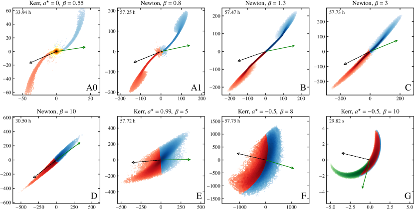
Our simulations produced a large variety of morphological classes for the tidal debris stream, some of which have not yet been presented in the literature. Based on geometry alone, we find that tidal disruptions may result in seven distinct morphological classes (see Fig. 3):
-
Class A: a surviving core surrounded by two tidal arms, without (A0) or with (A1) tidal lobes at the end ();
-
Class B: a thin, well-defined tidal bridge and two well-defined tidal lobes at the end; no visible core ();
-
Class C: a thick, poorly-defined tidal bridge, with two poorly-defined tidal lobes that span most of the length of the bridge ();
-
Class D: a thin, airfoil-shaped stream (Newtonian: );
The Kerr cases additionally result in:
-
Class E: two nearly-triangular, overlapping tidal lobes with no tidal bridge in between (Kerr only: );
-
Class F: a thick stream that is only accreting from its inner part (Kerr only: , but highly dependent on the spin);
-
Class G: a spiral that is accreting from its near-end and that is expanding ballistically (Kerr only: , again depending on the spin).
At low , the Newtonian and relativistic encounters are similar, passing progressively through stages A, B, and C; however, in so far as the relativistic encounters are more disruptive in terms of the mass removed from the star, they reach stages B and C at lower impact parameters.
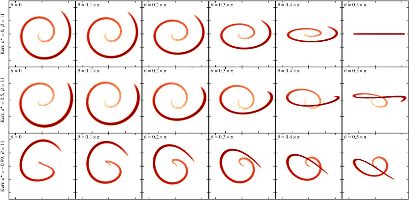
After (), Newtonian and relativistic encounters become qualitatively different: the Newtonian encounters with are similar, resulting in virtually identical airfoil-shaped debris streams that expand adiabatically. For the encounters in Kerr, however, we observe several new morphological classes, all of them ultimately linked to the individual relativistic precession of the fluid elements: up to , the tidal tails merge into a single, double-triangular shaped stream with no tidal bridge. After that, up until , the debris takes the shape of a very thick, banana-shaped stream that accretes from its inner part. Above , the stream becomes a spiral expanding ballistically, with one end “anchored” to the BH.
We note that the relativistic debris in panels E and F in Fig. 3 exhibits a considerably larger width than in the Newtonian case, due to the differential periapsis shifts imparted on the different fluid streams during the periapsis passage. The prospect of observing such debris streams is promising: the unbound material keeps expanding and cooling adiabatically, generating an optical transient from hydrogen recombination (Kasen & Ramírez-Ruiz, 2010). It would be plausible to make the assumption that the axis ratio of the debris in the orbital plane, in the presence of strong periapsis shift, is of order 1, as can be seen in classes E and F, instead of , as was assumed by Kasen & Ramírez-Ruiz (2010), and which is in agreement with our Newtonian simulations represented by class D. In this case, both the expansion time , defined by Kasen & Ramírez-Ruiz (2010) in their Eq. (8) as scaling with , and the time at which the transient is expected to occur, , given in their Eq. (19) with the same scaling, would be reduced by a factor of . In order to test this, we extract the times at which the mean and maximum temperatures of the debris stream drop below in two simulations with (Newtonian and Kerr with ). For the mean temperatures, we find the Newtonian time to be h, compared to h for Kerr, representing a speed-up of , in agreement with our very simple order-of-magnitude analytical estimate.
If, instead, we consider the maximum temperature, the contrast is much larger: in the Newtonian case, the maximum temperature, at the centre of the debris stream, only drops below after days, while in the Kerr case it takes merely days, representing a speed-up of more than . In any case, both effects are greatly diminished for , where the periapsis shift is not strong enough to generate the 1:1 aspect ratio of the debris in the orbital plane.
Another scenario is the production of a -ray afterglow following the collision of the expanding debris with molecular clouds (Chen, Gómez-Vargas & Guillochon, 2016). The effect of relativistic periapsis shift is to significantly increase the solid angle of the unbound ejecta, reducing the time it takes to end the free expansion and begin the Sedov-like phase, as predicted by Khokhlov & Melia (1996) though never followed-up with three-dimensional relativistic simulations. The velocities of the ejecta are similar in the Newtonian and relativistic simulations (since the parabolic velocities are comparable, and of the order of few percent of the speed of light), however the expansion velocity (relative to the centre of mass) is higher in the relativistic simulations by 50 per cent (below ), 10 per cent (for ), and up to 300 per cent (in deeper encounters); the effect is enhanced for retrograde orbits, and diminished for prograde orbits, as compared to the Schwarzschild case. This would be expected to significantly enhance the radio signal that is produced once the unbound part is braked by the ambient gas, as the total power radiated in bremsstrahlung scales with the square of the velocity (Landau & Lifshitz, 1971).
For case G, the spiral eventually ends up winding multiple times around the BH. The spiral shown for class G is much thinner than the debris stream in classes E and F, but note that the time of the snapshot is a mere 30 seconds after the periapsis passage, just before the plunge of the most bound particle into the event horizon, as compared with hours for E and F. The spiral, however, continues to expand because of the differential periapsis shift, and it eventually reaches a comparable width to cases E and F (based on ballistic extrapolation). Running the full simulation, however, would be problematic, due to the imperative of accurately treating the plunge and the second periapsis passage, which is outside the scope of this paper.
We also note that we have found the bound and unbound debris to be mixed (as previously observed in the simulations of Cheng & Bogdanović, 2014), under the action of the different periapsis shifts. This contrasts with the Newtonian case, where the bound and unbound debris are always separated by the initial trajectory of the centre of mass. The effect only appears in very close () encounters, where a crescent-shape debris stream is formed (as seen before in Laguna et al., 1993b; Kobayashi et al., 2004; Cheng & Bogdanović, 2014; TGRM+17). Due to the same mixing, a significant part of the plunging material (which is marked with green in plot G of Fig. 3) may be energetically unbound, invalidating the premise (otherwise valid for the Newtonian case) that “half” of the debris always escapes (see Table 3). Nevertheless, we observe that the ratio of bound to unbound plunging material is not 1, but ranges from (for ) to (for ). The case produces a negligible amount of plunging material, since the periapsis is further from the event horizon. The most dramatic effect which we see, three-dimensional spirals, appears due to Lense–Thirring precession, i.e. only around Kerr BHs with ; see Fig. 4; we have first presented such a geometry in Sec. 5.3 of TGRM+17.
| Spin | Plunging [%] | Bound [%] | Unbound [%] | |
|---|---|---|---|---|
| 9 | 0.38 | 47.89 | 51.73 | |
| 10 | 23.60 | 34.25 | 42.15 | |
| 11 | 48.52 | 20.57 | 30.91 | |
| 9 | 0.26 | 48.01 | 51.73 | |
| 10 | 23.06 | 34.21 | 42.73 | |
| 11 | 49.05 | 19.61 | 31.34 | |
| 0.0 | 9 | 0.07 | 48.53 | 51.40 |
| 0.0 | 10 | 5.95 | 44.66 | 49.39 |
| 0.0 | 11 | 38.96 | 25.43 | 35.61 |
| 0.5 | 9 | 0.23 | 48.89 | 50.88 |
| 0.5 | 10 | 0.22 | 48.17 | 51.61 |
| 0.5 | 11 | 2.83 | 46.87 | 50.30 |
| 0.99 | 9 | 0.31 | 48.99 | 50.70 |
| 0.99 | 10 | 0.32 | 48.70 | 50.98 |
| 0.99 | 11 | 0.30 | 48.17 | 51.53 |
We observe that in the Kerr case the debris stream tends to puff up due to Lense–Thirring precession, an effect that does not exist in Newtonian simulations. This may have implications for how long such a TDE can avoid detection, as the general prediction is that a thin-enough stream will avoid self-intersection for many orbital periods (Guillochon & Ramírez-Ruiz, 2015b).
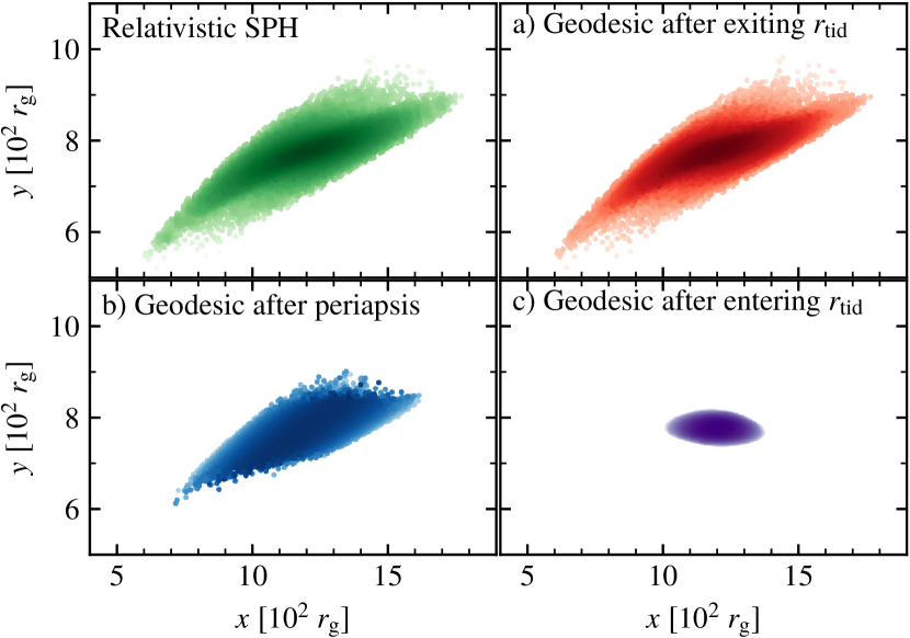
While reviewing how nodal precession may prevent the self-intersection of the debris stream, Stone et al. (2019) pointed out that streams in SPH simulations with adiabatic Equations of State (EOS) tend to puff up quickly due to heating from internal shocks, and quickly circularize, while streams with isothermal EOS tend to remain narrower for a longer time, avoiding circularization for up to 10 orbital periods of the most-bound debris (). Based on the typical temperatures, densities and opacities of the bound TDE debris stream, it is unlikely that it could be well described by an isothermal EOS, since it is highly opaque to radiation. Nevertheless, the concern that SPH simulations tend to produce puffed up TDE debris streams is valid, and we would like to address it, since a number of the results in this paper originate in the wider debris streams we obtain for relativistic TDEs. In our simulations, since we only treat the first stage of the disruption, internal shocks only occur during the strong compression experienced during the first periapsis passage. In addition, the debris streams we obtain are much narrower in the vertical direction than in the orbital plane (with typical ratios between 10 and 100), and in any case remain much narrower in the Newtonian case than in Kerr (with typical ratios for classes E and F vs class D, see Fig. 3), all pointing towards the thickening being a relativistic, rather than hydrodynamic effect.
Still, in order to test numerically that the puffing up is solely the result of geodesic motion, and that hydrodynamic forces do not affect the stream’s evolution (at least not before the second periapsis passage), we have also run three control simulations of a complete disruption (Kerr, , ), by taking a snapshot: a) as the star exits the tidal radius after disruption, b) just after the first periapsis passage, and c) as the star enters the tidal radius before disruption, switching off the self-gravity and hydrodynamic forces, and letting the particles evolve on ballistic trajectories alone. The results at the end of the simulations (at the same time as the SPH case, hours after the periapsis passage) are shown in Fig. 5. We observe that cases a) and b) yield similar results, but only case a) is virtually identical to the original simulation, showing that the constants of motion do evolve for some time after the bounce, but settle in by the time the star exits the tidal radius. The case c) utterly fails to reproduce the geometry of the debris stream, proving that the periapsis passage is crucial in determining how the energy and angular momentum are redistributed, and so the frozen-in model cannot be applied when entering to determine the stream geometry, at least for deep encounters. The results also show that the expansion of the debris stream is due to geodesic motion alone, as even if the constants of motion are frozen at periapsis, the resulting debris stream has a comparable thickness to the one from the full simulation, and much thicker than in the Newtonian case.
3.2.3 Energy spread
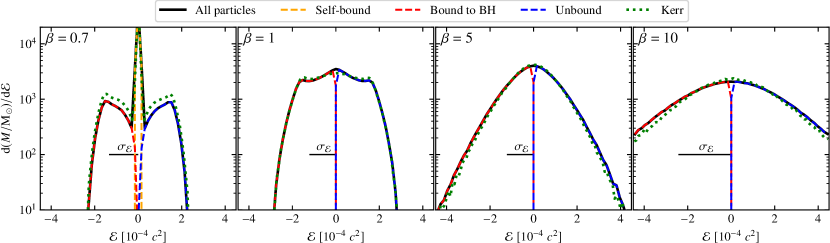
We find that the energy distribution () is not flat around except for a narrow range of impact parameters around (Fig. 6), when most of the matter resides in the thin and dense tidal bridge (class C in Fig. 3). For weaker encounters, when the core of the star survives, exhibits broad wings that may evolve at late times under the gravitational influence of the self-bound core; for strong disruptions, above , the logarithmic histogram of can be fitted remarkably well by a generalized Gaussian function, with the Gaussian parameters and being smooth functions of , as shown in Appendix A.
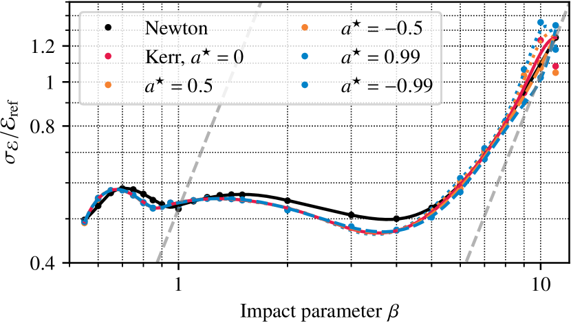
The spread in orbital mechanical energies, calculated as the standard deviation of the energy distribution, , exhibits little variation with until after , where it starts approaching the theoretical predictions of the standard frozen-in model, (Fig. 7). These results are somewhat in contradiction with those recently presented by Steinberg et al. (2019), who found that above the spread in energy is nearly insensitive with . Apart from using very different codes and computing the energy spread in different ways, it is difficult to understand well the origin of this difference, as they do not present histograms of the energy distribution. We strongly emphasize that the energy spread, in itself, does not offer much information about the disruption, in general, or the fallback rate, in particular, unless it is coupled with the (quite erroneous) assumption that the energy distribution is flat, which only holds around .
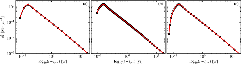
3.3 Fallback
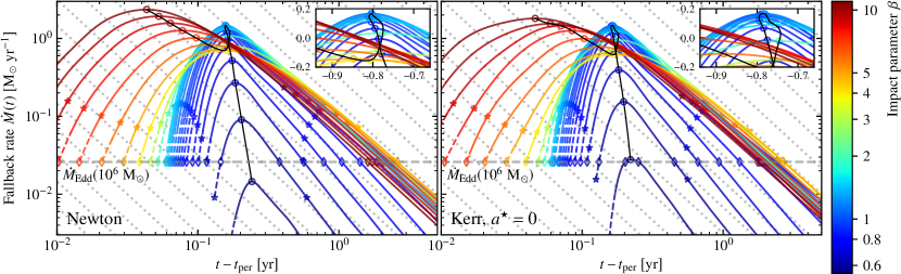
In Fig. 8 we present the fallback rates, , for the Newtonian simulations (left panel) and for the Kerr case with (right panel). The procedure for binning the data is discussed at length in Appendix B. The log–log plot is similar to the one presented in Fig. 5 of GRR13, although the parameter range is now extended to . The fact that, up to , the results match so well the ones from the reference paper is a non-trivial test of both, since the two sets of simulations have been performed with different codes, using different formalisms (high-resolution, grid-based simulations, with a multipole gravity solver, in the rest frame of the star, vs medium-resolution, global, tree-based SPH particle simulation), different ways of setting up the initial conditions and of postprocessing the data, etc. We even reproduce the feature of discovered by GRR13 at around , where the initial trend at low , towards earlier and higher peaks with increasing , reverses to later and lower ones. We find, however, that the trend reverses again around , where the peak starts shifting to significantly higher accretion rates and to earlier times. Our explanation for this behaviour is related to the occurrence of shocks during the periapsis passage, which does not happen at lower , as will be discussed later on.
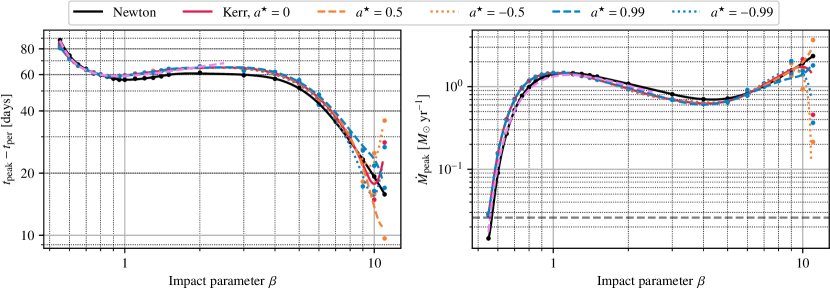
In Fig. 9 we present the times and magnitudes of the peak fallback rate, and . For , the results for the Newtonian simulations are in agreement with Fig. 12 of GRR13, whose fit curves are overplotted with a dashed purple line. Our results also agree with the tidal disruptions of Cheng & Bogdanović (2014), who concluded that Newtonian rates have a slightly earlier rise, while GR rates exhibit: a more gradual rise, a higher peak, and a later rise above the Eddington limit. However, the trend reverses after , with the peak fallback increasing and occurring at earlier times. We find to be significantly higher and to be earlier than the predictions of the frozen-in model, consistent with the recent findings of Wu, Coughlin & Nixon (2018).
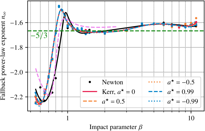
In Fig. 10 we plot the slope of the fallback rate at late times. Again, the data are fairly similar to what GRR13 presented in their Fig. 7. At high , the trend does not disappear, and the slope remains very close to .
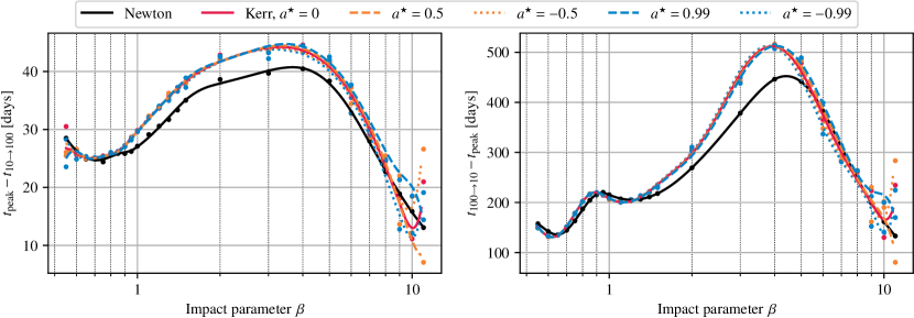
In Fig. 11, we plot the time of rise from 10 to 100 per cent of (, left panel) and the time of decay from 100 to 10 per cent of (, right panel). These quantities, although not customarily presented in the literature on numerical TDEs, may very much be of interest for the analysis of observational data, as they are a good representation of how broad the fallback curves are, and of how quickly they rise and fall. Here is where we find the biggest relativistic effects, most noticeable at moderate (between and 5). There, the relativistic fallback rates take few days longer to reach the peak from per cent of its value, and significantly longer ( few months) to decay.
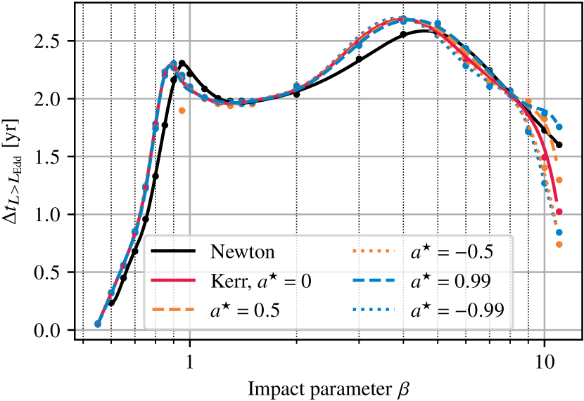
In Fig. 12, we plot the duration of super-Eddington fallback rate. This is not as helpful a quantity as and , since it depends non-trivially on the combination of the BH mass and the shape of the fallback rate curve. The trends that we find for our disruptions by a BH are that: a) relativistic super-Eddington fallback lasts from few months (for ) to years (for larger ) longer than in the Newtonian case; b) the duration of super-Eddington fallback is severely reduced in the high- relativistic encounters, due to the large amount of material that plunges directly into the BH; c) for moderate disruptions, the duration in relativistic encounters may be longer by a month than in the Newtonian case.
To date, the most comprehensive numerical investigation of the TDE fallback process across a wide range of impact parameters has been undertaken in GRR13, in whose Appendix A the authors present fitting parameters for , , and , as functions of , scaled with , and , and with separate fittings for and . These fits have proven invaluable in subsequent detections of TDE flares (e.g., Gezari et al., 2015; Leloudas et al., 2016), and have helped narrow down the parameter space of those events. In Appendix A we present an extended range of fit formulae, based on the simulations in this paper, which extends the ones given in GRR13 to larger (up to 11) and to rotating black holes.
4 Discussion
A comparative look at most of the plots in this paper reveals that, depending on the impact parameter , tidal disruptions fall into three categories (we will illustrate with values of corresponding to ; note that the exact values of are different for other equations of states, most notably for polytropes with , although we expect the trend itself to be unchanged).
4.1 Weak disruptions
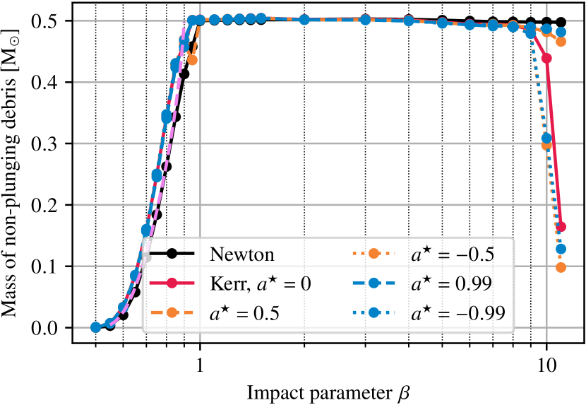
At low (), the star suffers a partial disruption. The mass fraction removed from the star and bound to the black hole varies greatly, ranging from around to at the disruption limit (Fig. 13; the exact value of greatly depends on , see GRR13); in the relativistic disruptions, more mass is stripped from the core than in the Newtonian case, from per cent more (at ) to per cent more (at ), in agreement with the pseudo-relativistic simulations of Gafton et al. (2015, Fig. 3; note that the effect is greatly exacerbated for larger BH masses). The effect of the BH spin is small but consistent, with per cent less mass in the surviving self-bound core for and about per cent more mass in the surviving self-bound core for as compared to .
The morphology of the tidal debris consists of a surviving core and two tidal tails (A0 and A1 in Fig. 3); the time to peak fallback rate is long, of the order of –3 months, and the fallback rate varies significantly, from at to at (Fig. 9); the relativistic simulations yield up to twice the fallback rate for the lower range of . The durations of the rise and decay of the fallback rate (quantified as the time it takes to get to 10 per cent of to , and back) are long and scale inversely with (Fig. 11). The duration of super-Eddington flow is highly variable (Fig. 8), from months for to years for . The energy spread is relatively high; the energy distribution consists only of the tidal tails, which are roughly centred around (Fig. 6) and quickly drop towards , predicting a sudden drop in the fallback curve. The long-term fallback exponent, , is significantly steeper than for very weak encounters (), and milder than close to the disruption limit () (Fig. 10); the reason for this is connected to the influence of the surviving core, and was explained at length in GRR13. We find the relativistic trend very similar, although is shifted to lower as compared to the Newtonian case.
4.2 Moderate disruptions
At moderate (), the star is disrupted completely, but remnants of self-gravitating cores remain: morphologically, in the form of a thin tidal bridge, and energetically, in the form of a flat central distribution and “wings” in the energy histogram. The tidal bridge is kept narrow by self-gravity, but at the two ends it broadens into two tidal tails with or without lobes (B and C in Fig. 3). The time to peak is shorter than for very weak disruptions ( 60 days), and the peak fallback rate is higher (by about one order of magnitude), but the trend reverses around , as first noted in GRR13, and also visible in the inset plots in Fig. 8); from that point, the fallback rate decreases and the time to peak increases with , reaching a minimum around (corresponding to the narrowest point in the spread in Fig. 10). The times of the rise and decay of the curve are very large, reaching a maximum around ( 45 days for the rise and 500 days for the decay); these encounters last the longest (as measured from to ), with relativistic effects prolonging them even further, by up to per cent around . The duration of super-Eddington flow is also very long, surpassing 2.5 years for rotating black holes with . The energy spread is small, with the lowest point occurring around ; the energy histogram consists of a relatively flat plateau of width where most of the mass is located (the tidal bridge), and has very little mass outside of it (in the tidal tails). In this regime, the long-term fallback rate slope settles to the canonical and exhibits virtually no variation with .
4.3 Strong disruptions
At high (), the star is fully disrupted; for Newtonian encounters, the morphology is a long stream, devoid of tidal tails or any other distinguishing features (D in Fig. 3); for the Kerr case, the debris is much thicker, with (E) or without (F) features reminiscent of the tidal tails; for non-equatorial orbits, the nodal precession creates three-dimensional spiral-like debris distributions (G) that move ballistically; due to the different shifts imparted at periapsis, the resulting structure is expected to thicken significantly in time.
The time to peak is very short (of the order of few weeks), and the fallback rate is very high, surpassing for the deepest encounters; this, however, is not the case in very close relativistic encounters, where a significant fraction of the star may plunge into a black hole and be promptly accreted (see Table 3), leaving less material to fall back and circularize. The energy spread is large, and it shows a power law dependence on , only slightly milder than the predicted by the original frozen-in theory; the logarithmic energy distribution assumes a nearly Gaussian shape, whose parameters can be well characterized in terms of alone. The fallback exponent remains very close to .
4.4 What happens at ?
We believe that the qualitative change in the disruption around is related to the shock that forms due to strong compression: at , the star is not compressed at all, and it is disrupted smoothly, due to the resonant quadrupole oscillations induced by the tidal field of the BH; there is no real bounce wave to steepen into a shock, because the fluid pressure has enough time to continuously react to the (mild) geodesic compression during the periapsis passage. At very large , however, the strong compression is halted by a shock, which then rebounds and travels to the surface of the star, as clearly confirmed in previous simulations (e.g., Guillochon et al., 2009 for and ). It follows, then, that there must be a boundary, in between full disruptions without compression or shock (at ) and full disruptions with large compression followed by a shock (which we know happens at ). This has been hinted at in Sec. 5.2 of TGRM+17, but not fully discussed. Note also that Rosswog et al. (2009) found a threshold value for detonating white dwarfs around , which would be consistent with the above interpretation.
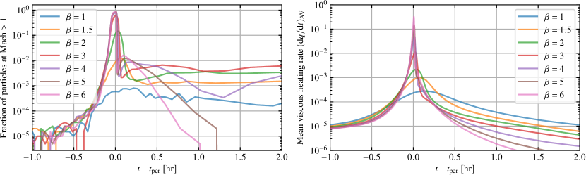
We look for the presence of shocks in two ways: first, with the geometrical shock-detection method for SPH presented by Beck, Dolag & Donnert (2016). In Fig. 14 (left panel) we plot the fraction of SPH particles that have a Mach speed larger than 1, as computed with the formalism described in Section 2 of that paper, as a function of time elapsed since periapsis, for seven Newtonian simulations ranging from to . We see that for , virtually the entire star is shocked right after the periapsis passage (with the curves being nearly identical for all ), while for less than 0.1 per cent of the star experiences Mach at periapsis. The actual location of the shock also differs: at low , the shock occurs in the tidal tails (as discussed before by Lodato et al., 2009), and the fraction of shocked particles is maintained at a level above per cent long after disruption ( few hours), with additional shocks occurring as a result of tidally-induced, non-linear stellar pulsations. On the other hand, at high (), the shock occurs throughout the entire star during the first periapsis passage; as the debris stream is now devoid of tidal tails and is merely expanding homologously, the fraction of shocked particles quickly drops by several orders of magnitude within an hour after disruption.
We also analyse the viscous heating rate , representing the contribution of the SPH artificial viscosity to the energy equation, which is a proxy for the entropy generated in the shock. In Fig. 14 (right panel) we plot the average , calculated for all SPH particles in the simulations with to , as a function of time elapsed since periapsis. We see that for the case, the average is three orders of magnitude larger than for , confirming the generation of significantly more shock entropy for the deeper encounters. The rise of the curve is also very abrupt (it rises by three orders of magnitude within minutes), and the peak is sharp at (lasting of the order of few minutes), but much softer for (lasting of the order of an hour). After the shock at periapsis subsides, we see the same trend as in the other panel: the low encounters result in higher post-periapsis shock indicators (in this case, the average 1 hour after the periapsis passage is decreasing with increasing ), related to long-term oscillations induced in the tidal tails.
Once the shock rebounds and travels through the star, it redistributes energy and angular momentum between the centre and the surface (the shock heating of the surface with energy from the stellar core may, indeed, even be responsible for a short X-ray transient, see Guillochon et al., 2009 and Yalinewich et al., 2019). What we would expect to see in such a case would be a complete loss of all the “features” in the energy and angular momentum histograms. At , the centre of is relatively flat (Fig. 6), corresponding to a tidal bridge whose fluid elements are imparted an orbital energy comparable to the one predicted by the frozen-in theory, while the two wings corresponding to the tidal lobes have a more peaked distribution); on the other hand, for , where the entire star is shocked, we would expect the energy distribution to be more Gaussian-like.
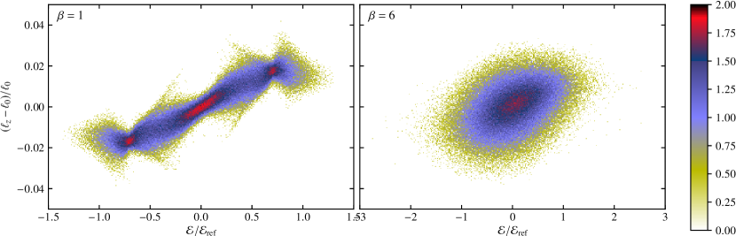
Indeed, in Fig. 15 we provide scatter plots of the energy and angular momentum , normalized by the reference energy spread and the initial angular momentum , respectively, for two Kerr simulations with and impact parameters (left panel) and (right panel). While the simulation yields a distribution similar to the one extracted by Cheng & Bogdanović (2014) from their relativistic simulations, with various features in the shape of the scatter plot, the simulations results in a featureless, normal distribution in both energy and angular momentum.
4.5 Relativistic effects
We analyse our results through the points of view of two opposite theoretical predictions. On the one hand, Kesden (2012), based on the model of an undisturbed star at periapsis (similar to the frozen-in model), argued that GR disruptions would be stronger for the same , producing a larger spread in energies and resulting in earlier peak times and higher peak rates (by up to a factor of two), more so for stars on retrograde orbits; our simulations do not support this conclusion. On the other hand, we find the argument of Servin & Kesden (2017) convincing: since the gravitational potential is steeper in GR (i.e., the tidal forces are stronger), the star will be disrupted higher in the potential well (i.e., further from the black hole), resulting in a smaller spread in specific energies. This creates the opposite result, of lower rates, later peak times, and a broader shape for the curve, in agreement with our findings and with the few previous relativistic studies (e.g., Cheng & Bogdanović, 2014). The two competing effects (steeper potential but earlier disruption) partially cancel out to yield relatively similar energy distributions and return rates (as seen before in Figures 9 and 11 of TGRM+17), making it more difficult to discriminate between a relativistic and a Newtonian encounter based solely on the mass return rate. The corrections to the shape of the debris fallback rate are also minor, and are strongest around .
On the other hand, the effect of GR on the morphology of the debris stream is more significant, even in weak encounters (at low ), as the differential periapsis shifts create much wider debris streams. In so far as the observational prospects are concerned, we believe it much more likely to see the effects of GR in aspects other than the fallback rates, such as:
-
(a)
the optical transient generated through recombination in the more expanded unbound debris stream;
-
(b)
the bremsstrahlung radiation resulting from the breaking of the expanding debris stream by the ambient gas;
-
(c)
the -ray signature from the collision of the expanding unbound debris with molecular clouds;
-
(d)
the X-ray signature of the shock breakout resulting from multiple bounces at periapsis;
-
(e)
the longer durations of super-Eddington flow, and longer times of rise () and decay ();
-
(f)
the increased disruption rate due to the stronger disruptions at low ;
-
(g)
the faster circularization, due to the self-crossing of the debris stream closer to the BH and at higher angles than in the Newtonian case.
5 Conclusions
In this paper, we presented the results of relativistic SPH simulations of tidal disruptions of stars by rotating supermassive black holes, for penetration parameters between and , and black hole spins between and . As expected, we found that general relativity particularly affects deep encounters, within a few event horizon radii, as follows: the strong (periapsis and nodal) precession creates debris stream geometries impossible to obtain with the Newtonian equations (such as three-dimensional spirals winding multiple times around the black hole, Fig. 4); part of the fluid can be launched on plunging orbits, which reduces the fallback rate and decreases the mass of the resulting accretion disc (by as much as 80 per cent in the deepest encounters with retrograde spin, Fig. 13); a suite of compression and bounce episodes at periapsis in very deep relativistic encounters (Fig. 2) may generate distinctive X-ray signatures resulting from the associated shock breakout; we also found that disruptions can even occur inside the marginally bound radius, if the enhanced angular momentum spread launches part of the debris on non-plunging orbits (as is the case of all the simulations with and ).
Perhaps surprisingly, we also found relativistic effects to be important in weak disruptions, where the balance between self-gravity and the tidal force is very close to equilibrium. In this case, the otherwise minor relativistic effects can have decisive consequences on the qualitative outcome of the disruption.
In between, where the star is fully disrupted but relativistic effects are not extreme, the difference is less conspicuous and resides mostly in a gentler rise of the fallback rate, a later peak and a broader return rate curve, in agreement with the few previous relativistic simulations. However, even in the case of moderately strong encounters, we found that the differential periapsis shift creates much thicker debris streams than in the Newtonian case, both in the bound part (possibly speeding up the circularization) and in the unbound part (speeding up the production of the recombination transient by a factor of two, and enhancing the interaction of the ejecta with the interstellar medium).
In Appendix A we provided fit formulae for various properties of the disruption (such as maximum compression at periapsis, shape and spread of the energy distribution) and potential observables (such as the peak fallback rate, the times of rise, peak and decay, and the duration of the super-Eddington fallback phase) as a function of the impact parameter and the black hole spin.
In Appendix B we discussed our strategy for binning the return times of the SPH particles and fitting a spline to the resulting histogram, so as to generate a continuous function based on which most quantities discussed in this paper were computed.
Acknowledgements
The authors would like to thank John C. Miller, Elad Steinberg, and the anonymous referee for valuable comments on the manuscript. We would also like to thank Emilio Tejeda and James Guillochon for many insightful discussions on the topic of the paper. S.R. has been supported by the Swedish Research Council (VR) under grant number 2016-03657 3, by the Swedish National Space Board under grant number Dnr. 107/16 and by the research environment grant “Gravitational Radiation and Electromagnetic Astrophysical Transients” (GREAT) funded by the Swedish Research council (VR) under Dnr. 2016-06012. Support from the COST Actions on neutron stars (PHAROS; CA16214) and black holes and gravitational waves (GWerse; CA16104) are gratefully acknowledged. The simulations and postprocessing have in part been carried out on the facilities of the North-German Supercomputing Alliance (HLRN) in Hannover, Göttingen and Berlin, and of the PDC Centre for High Performance Computing (PDC–HPC) in Stockholm.
References
- Anninos et al. (2018) Anninos P., Fragile P. C., Olivier S. S., Hoffman R., Mishra B., Camarda K., 2018, ApJ, 865, 3, 1808.05664
- Bardeen et al. (1972) Bardeen J. M., Press W. H., Teukolsky S. A., 1972, ApJ, 178, 347
- Beck et al. (2016) Beck A. M., Dolag K., Donnert J. M. F., 2016, MNRAS, 458, 2080, 1511.07444
- Bicknell & Gingold (1983) Bicknell G. V., Gingold R. A., 1983, ApJ, 273, 749
- Bogdanović et al. (2004) Bogdanović T., Eracleous M., Mahadevan S., Sigurdsson S., Laguna P., 2004, ApJ, 610, 707, astro-ph/0404256
- Bonnerot et al. (2016) Bonnerot C., Rossi E. M., Lodato G., Price D. J., 2016, MNRAS, 455, 2253, 1501.04635
- Carter & Luminet (1983) Carter B., Luminet J.-P., 1983, A&A, 121, 97
- Chandrasekhar (1939) Chandrasekhar S., 1939, An introduction to the study of stellar structure
- Chen et al. (2016) Chen X., Gómez-Vargas G. A., Guillochon J., 2016, MNRAS, 458, 3314, 1512.06124
- Cheng & Bogdanović (2014) Cheng R. M., Bogdanović T., 2014, PRD, 90, 064020, 1407.3266
- Cheng & Evans (2013) Cheng R. M., Evans C. R., 2013, PRD, 87, 104010, 1303.4129
- Evans et al. (2015) Evans C., Laguna P., Eracleous M., 2015, ApJ, 805, L19, 1502.05740
- Frolov et al. (1994) Frolov V. P., Khokhlov A. M., Novikov I. D., Pethick C. J., 1994, ApJ, 432, 680
- Gafton et al. (2015) Gafton E., Tejeda E., Guillochon J., Korobkin O., Rosswog S., 2015, MNRAS, 449, 771, 1502.02039
- Gezari et al. (2015) Gezari S., Chornock R., Lawrence A., Rest A., Jones D. O., Berger E., Challis P. M., Narayan G., 2015, ApJ, 815, L5, 1511.06372
- Golightly et al. (2019) Golightly E. C. A., Coughlin E. R., Nixon C. J., 2019, ApJ, 872, 163, 1901.03717
- Guillochon & Ramírez-Ruiz (2013) Guillochon J., Ramírez-Ruiz E., 2013, ApJ, 767, 25, 1206.2350
- Guillochon & Ramírez-Ruiz (2015a) Guillochon J., Ramírez-Ruiz E., 2015a, ApJ, 798, 64
- Guillochon & Ramírez-Ruiz (2015b) Guillochon J., Ramírez-Ruiz E., 2015b, ApJ, 809, 166, 1501.05306
- Guillochon et al. (2009) Guillochon J., Ramírez-Ruiz E., Rosswog S., Kasen D., 2009, ApJ, 705, 844, 0811.1370
- Haas et al. (2012) Haas R., Shcherbakov R. V., Bode T., Laguna P., 2012, ApJ, 749, 117, 1201.4389
- Hayasaki et al. (2013) Hayasaki K., Stone N., Loeb A., 2013, MNRAS, 434, 909, 1210.1333
- Hayasaki et al. (2016) Hayasaki K., Stone N., Loeb A., 2016, MNRAS, 461, 3760, 1501.05207
- Hunter (2007) Hunter J. D., 2007, Comput. Sci. Eng., 9, 90
- Jones et al. (2001) Jones E., Oliphant T., Peterson P., et al., 2001, SciPy: Open source scientific tools for Python, http://www.scipy.org/
- Kagaya et al. (2019) Kagaya K., Yoshida S., Tanikawa A., 2019, preprint, 1901.05644
- Kasen & Ramírez-Ruiz (2010) Kasen D., Ramírez-Ruiz E., 2010, ApJ, 714, 155, 0911.5358
- Kesden (2012) Kesden M., 2012, Phys. Rev. D, 86, 064026, 1207.6401
- Khokhlov & Melia (1996) Khokhlov A., Melia F., 1996, ApJL, 457, L61
- Kobayashi et al. (2004) Kobayashi S., Laguna P., Phinney E. S., Mészáros P., 2004, ApJ, 615, 855, astro-ph/0404173
- Komossa (2015) Komossa S., 2015, J. High Energ. Astrophys., 7, 148, 1505.01093
- Laguna et al. (1993a) Laguna P., Miller W. A., Zurek W. H., 1993a, ApJ, 404, 678
- Laguna et al. (1993b) Laguna P., Miller W. A., Zurek W. H., Davies M. B., 1993b, ApJL, 410, L83
- Landau & Lifshitz (1971) Landau L. D., Lifshitz E. M., 1971, The classical theory of fields
- Leloudas et al. (2016) Leloudas G., et al., 2016, Nature Astronomy, 1, 0002, 1609.02927
- Lodato et al. (2009) Lodato G., King A. R., Pringle J. E., 2009, MNRAS, 392, 332, 0810.1288
- Lodato et al. (2015) Lodato G., Franchini A., Bonnerot C., Rossi E. M., 2015, J. High Energ. Astrophys., 7, 158
- Luminet & Marck (1985) Luminet J.-P., Marck J.-A., 1985, MNRAS, 212, 57
- Luminet & Pichon (1989) Luminet J.-P., Pichon B., 1989, A&A, 209, 103
- Mockler et al. (2019) Mockler B., Guillochon J., Ramírez-Ruiz E., 2019, ApJ, 872, 151, 1801.08221
- Monaghan (2005) Monaghan J. J., 2005, Rep. Progr. Phys., 68, 1703
- Phinney (1989) Phinney E. S., 1989, in Morris M., ed., IAU Symp. Vol. 136, The Center of the Galaxy. p. 543
- Price (2007) Price D. J., 2007, PASA, 24, 159, 0709.0832
- Rees (1988) Rees M. J., 1988, Nature, 333, 523
- Rosswog (2009) Rosswog S., 2009, New Astron. Rev., 53, 78, 0903.5075
- Rosswog (2015) Rosswog S., 2015, Living Rev. Comput. Astrophys., 1, 1, 1406.4224
- Rosswog et al. (2008a) Rosswog S., Ramírez-Ruiz E., Hix W. R., Dan M., 2008a, Comput. Phys. Commun., 179, 184, 0801.1582
- Rosswog et al. (2008b) Rosswog S., Ramírez-Ruiz E., Hix W. R., 2008b, ApJ, 679, 1385, 0712.2513
- Rosswog et al. (2009) Rosswog S., Ramírez-Ruiz E., Hix W. R., 2009, ApJ, 695, 404, 0808.2143
- Runge (1901) Runge C., 1901, Z. Math. Phys., 46, 224
- Sa̧dowski et al. (2016) Sa̧dowski A., Tejeda E., Gafton E., Rosswog S., Abarca D., 2016, MNRAS, 458, 4250, 1512.04865
- Servin & Kesden (2017) Servin J., Kesden M., 2017, PRD, 95, 083001, 1611.03036
- Shiokawa et al. (2015) Shiokawa H., Krolik J. H., Cheng R. M., Piran T., Noble S. C., 2015, ApJ, 804, 85, 1501.04365
- Steinberg et al. (2019) Steinberg E., Coughlin E. R., Stone N. C., Metzger B. D., 2019, MNRAS, 485, L146, 1903.03898
- Stone et al. (2013) Stone N., Sari R., Loeb A., 2013, MNRAS, 435, 1809, 1210.3374
- Stone et al. (2019) Stone N. C., Kesden M., Cheng R. M., van Velzen S., 2019, Gen. Relativ. Gravit., 51, 30, 1801.10180
- Tejeda et al. (2017) Tejeda E., Gafton E., Rosswog S., Miller J. C., 2017, MNRAS, 469, 4483, 1701.00303
- Wang & Merritt (2004) Wang J., Merritt D., 2004, ApJ, 600, 149, astro-ph/0305493
- Wu et al. (2018) Wu S., Coughlin E. R., Nixon C., 2018, MNRAS, 478, 3016, 1804.06410
- Yalinewich et al. (2019) Yalinewich A., Guillochon J., Sari R., Loeb A., 2019, MNRAS, 482, 2872, 1808.10447
- Zheng & Filippenko (2017) Zheng W., Filippenko A. V., 2017, Apj, 838, L4, 1612.02097
- van der Walt et al. (2011) van der Walt S., Colbert S. C., Varoquaux G., 2011, Comput. Sci. Eng., 13, 22, 1102.1523
Appendix A Fitting parameters
We have calculated updated fitting parameters for the four characteristic quantities that appear in the Appendix of GRR13: the peak fallback rate (), the time from the first periapsis passage to peak (), the fraction of mass lost by the star (), and the long-term slope of the fallback rate (). We also provide fitting parameters for several additional quantities: the time of rise of the fallback rate from 10 per cent of to (), the time of decay of the fallback rate from to 10 per cent of (), the duration of super-Eddington fallback (), the spread in the energy distribution , and the energy distribution .
The fits are given in terms of functions of the penetration factor (the first four being analogous to the , , and given by GRR13), and follow the scaling with the BH size , the stellar mass and radius , the radiative efficiency and the canonical energy spread (Eq. 1 with and ) given by GRR13 and Stone et al. (2019):
| (2) | ||||
| (3) | ||||
| (4) | ||||
| (5) | ||||
| (6) | ||||
| (7) | ||||
| (8) | ||||
| (9) | ||||
| (10) |
For we fit a generalized Gaussian function,
| (11) |
where is the expected mean specific energy after the disruption, is the gamma function, and the parameters and are given in Table 4 as and , respectively. Note that , and reduces the generalized Gaussian in Eq. 11 to the normal distribution with mean and variance .
We point out that while the Newtonian fits are straightforward (since the fit functions only depend on ), in the relativistic case the problem is a lot more complex: not only is the dependence on not strictly monotonic, but even in the absence of spin relativistic effects depend on the ratio. For instance, two encounters with the same will have very different curves for and (see Section 3 and in particular Fig. 3 of Gafton et al., 2015, where this point is clearly visible even for non-rotating BHs). This means that the scalings given above hold for Kerr only around , and will break down for much larger BH masses. In so far as the deviation from Newtonian curves (which scale with ) is due to relativistic effects (which scale with ), an alternative would be to fit the relativistic curves in terms of offsets from the Newtonian ones, and then give those offsets as functions of and of ).
For the plots in this paper, some of the time scales above were plotted in days, with the conversion being made assuming a Julian year, of 86 400 seconds each.
As opposed to GRR13, who determined their through via a ratio of polynomials fit, we chose to provide a B-spline representation of our data. This is motivated by a number of reasons: a) since our data extend to , it exhibits a more complicated trend, with various local extrema (in particular around , , and ). A higher order polynomial fit would be necessary to capture all of the trends in the data, making the procedure vulnerable to Runge’s phenomenon (Runge, 1901); a B-spline fit generally avoids this issue; b) both the coefficients and the knots of a B-spline are closely related to the actual data (i.e., to the and axis, respectively), while the coefficients of a polynomial (particularly in a ratio of polynomials) can grow arbitrarily high, and bear no relation to the data themselves (in particular, trying to fit another variable, such as the BH spin , to the coefficients, would not generally make sense); c) we determined that a very low precision (as low as 3 significant digits per coefficient) is sufficient to yield a virtually indistinguishable curve from the one constructed with coefficients given with machine precision (mostly because the coefficients are related to the -values); on the other hand, for a polynomial fit the coefficients need to be expressed with high precision, otherwise the fit cannot be reproduced (Guillochon & Ramírez-Ruiz, 2015a).
All B-spline curves used here are cubic (i.e., of order ) and valid on a specific interval . In general, a B-spline will have an arbitrary interior knots and border knots, which for simplicity are normally taken as equal to the boundary values ( and , respectively). The number of coefficients is . For brevity, we will not write down the border knots (which can be deduced from the limits of the domain).
| Quantity | Range of | Knots | Coefficients |
|---|---|---|---|
| [0.55, 11] | [0.65, 0.75, 0.85, 0.95, | [0.0147, 0.0201, 0.227, 0.807, 1.19, 1.36, 1.55, 1.29, 0.854, 0.578, 0.977, 1.75, 2.35] | |
| 1.0, 1.5, 2, 4, 7] | |||
| [0.55, 11] | Same as | [0.242, 0.206, 0.18, 0.166, 0.16, 0.155, 0.154, 0.167, 0.165, 0.164, 0.0798,0.0544, 0.0433] | |
| [0.50, 0.95] | [0.65, 0.75, 0.85] | [0.000242, , 0.0436, 0.356, 0.696, 0.882, 0.916] | |
| [0.55, 11] | [0.90, 0.95, 1.0, 1.4, 4] | [, , , , , , , , ] | |
| [0.55, 11] | Same as | [0.0781, 0.073, 0.0674, 0.0673, 0.0714, 0.0713, 0.0799, 0.1, 0.107, 0.12, 0.0664, 0.0442, 0.0359] | |
| [0.55, 11] | Same as | [0.431, 0.401, 0.337, 0.445, 0.575, 0.61, 0.541, 0.58, 0.895, 1.49, 0.691, 0.46, 0.364] | |
| [0.55, 11] | Same as | [0.234, 0.234, 0.594, 0.815, 1.85, 2.38, 1.93, 1.96, 2.15, 2.84, 2.12, 1.76, 1.6] | |
| [0.55, 11] | Same as | [0.497, 0.516, 0.588, 0.584, 0.551, 0.525, 0.557, 0.575, 0.522, 0.459, 0.682, 1.04, 1.25] | |
| [1, 11] | [1.5, 2, 4, 7 ] | [1.95, 2.13, 2.07, 1.86, 1.11, 1.76, 2.63, 3.13] | |
| [1, 11] | [1.5, 2, 4, 7] | [3.75, 7.2, 5.22, 2.94, 1.22, 1.85, 1.63, 1.91] | |
| [0.55, 11] | [0.65, 0.75, 0.85, 0.95, | [, , , | |
| 1.0, 1.5, 2, 3, 6, 9] | , , , | ||
| , , , | |||
| , ] | |||
| [0.55, 11] | Same as | [, , , , | |
| , , , , | |||
| , , , , | |||
| ,] | |||
| [0.50, 0.95] | [0.65, 0.75, 0.85] | [, , , | |
| , , , ] | |||
| [0.55, 11] | [0.90, 0.95, 1.0, 1.4, 4] | [, , , , | |
| , , , , ] | |||
| [0.55,11] | Same as | [, , , , | |
| , , , , | |||
| , , , , | |||
| ,] | |||
| [0.55,11] | Same as | [, , , , | |
| , , , , | |||
| , , , , | |||
| ,] | |||
| [0.55,11] | Same as | [, , , , , | |
| , , , , | |||
| , , ] | |||
| [0.55,11] | Same as | [, , , , | |
| , , , , , | |||
| , , , , ] | |||
| [1, 11] | [1.5, 2, 4, 7] | [, , , , , | |
| , , ] | |||
| [1, 11] | [1.5, 2, 4, 7] | [, , , , , | |
| , , ] |
The fits for the Newtonian and Kerr simulations are given separately in Table 4 in terms of B-spline knots and coefficients compatible with popular spline functions such as splev from the python library scipy. To illustrate this, the following python code snippet generates the curve based on ’s knots and coefficients from Table 4:
1 import numpy as np 2 from scipy.interpolate import splev 3 knots = [0.55, 0.55, 0.55, 0.55, 0.65, 0.75, 0.85, 0.95, 1.0, \ # Note the extra guard knots 4 1.5, 2.0, 4.0, 7.0, 11.0, 11.0, 11.0, 11.0] # (four on each side) 5 coeffs = [0.0147, 0.0201, 0.227, 0.807, 1.19, 1.36, 1.55, 1.29, \ 6 0.854, 0.578, 0.977, 1.75, 2.35] 7 order = 3 8 xaxis = np.linspace(0.55, 11, 1000) 9 yaxis = splev(xaxis, [knots, coeffs, order])
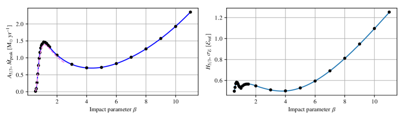
The resulting function, defined by the arrays xaxis and yaxis, is shown in Fig. 16 (left panel) as a solid blue line; the data points from our simulations are overplotted as filled black circles, while the fit from GRR13 is shown as a dashed purple line. In Fig. 16 (right panel) we repeat the same exercise, this time with . In both cases, the fit to the data is excellent, and accomplished with as little as 3 significant digits per coefficient.
Appendix B Binning procedure for the fallback rate
Once the return times to periapsis are calculated from the specific orbital energy (and, in the Kerr case, also from the angular momentum and the Carter constant, see, e.g., Appendix A of TGRM+17), one is left with a set of discrete values whose normalized histogram represents the mass return rate, . In order to convert the distribution of values (over all particles ) into a continuous function (as opposed to a discrete histogram), two steps are required: the binning of the data into a histogram, and the fitting of a sensible curve to the resulting histogram.
B.1 Choosing the bins
We found that the fit of quantities such as and is quite sensitive to how the data are binned and interpolated. In particular, both the rise part of the curve and the decay should be smooth and defined well enough so that one can reliably extract quantities before the peak (such as ) and after the peak (such as and ). While one could employ statistical analysis or machine learning techniques to solve this problem, we have attempted to devise a very simple procedure that still works well at low resolution ( particles, representing the bound half of the debris stream in our simulations).
In order to capture the long-term evolution of the curve, where both the times and the return rates can span several orders of magnitude, a good binning scheme should be logarithmic. Due to finite resolution and imperfect sampling, a naive histogram (e.g., with equal-width logarithmic bins) will tend to be very noisy if the number of bins is larger than , particularly in the decay part of the curve. For bins, the histogram may be quite smooth, but will fail to capture much of the rising part of the curve, and will also miss details of the peak (in particular the broken power-law typical of TDEs at ), as shown in panel (a) of Fig. 17. In the case of the very low- simulations (where only a very small fraction of the star becomes bound debris), the effect is even worse, to the point where the resulting curve hardly resembles a typical TDE fallback curve (quick rise, power-law decay).
An alternative to the equal-width bins would be to use an equal number of particles in each bin. This would sample reasonably well the rise and decay part of the curve, provided the number of particles per bin is small (e.g., 1000), but would quickly become noisy towards the peak of the curve, where most of the particles are concentrated, as shown in Fig. 17. Since these are competing effects, modifying the (fixed) number of particles in the bins would improve one of the two parts of the curve (rise+decay vs peak, i.e. low- vs high-resolution) at the expense of the other.
We decided, therefore, to take the best of these approaches: sample the rise and fall with a small number of particles per bin, and use few bins and a lot of particles per bin for the peak of the curve. In order to make the algorithm automatic and deterministic, we choose an initial number of particles for the first bin, at the beginning of the curve (i.e., starting at the particle with the shortest return time), and then successively increase the number of particles per bin until reaching a maximum . The same procedure is then applied starting at the last bin, at the other end of the curve (i.e., from the particle with the longest return time), also until is reached. Then, the remaining particles, around , are equally distributed into as few bins as necessary so as not to surpass in each bin. Of course, care is taken along the way not to distribute more particles than available, if is not reachable because there are very few particles, e.g., at very low .
There are various choices of how to increase the number of particles per
bin, of which we tested two:
a) multiplying the number of particles in the previous bin by a constant
, e.g., , until reaching :
| (12) |
b) increasing the number of particles in the previous bin by a constant , e.g., , until reaching :
| (13) |
The two methods give comparable results, but we have chosen b) as it is slightly better at sampling the low-density parts of the curve, where the exponential growth of is too fast.
Our experiments show that, for particles, , , and are good values, which minimize the noise in the histograms across the entire range of . An example of such a histogram is shown in panel (c) of Fig. 17. It is evident even at a glance that the rise of the curve is better sampled than in either of the other methods, the features of the peak are reproduced well, without any noise, while the decay part is sampled comparably to method (a), and is less noisy than in method (b).
B.2 Choosing a fit curve
Once a histogram is created, we fit a cubic spline through the histogram points in log–log space, which gives a smooth, continuous, and – most importantly – analytically differentiable function . We have experimented with using more complex, global functions inspired by the literature on supernova light curves (such as variant broken-power-law functions, see Zheng & Filippenko, 2017), but found them unsatisfactory in the case of TDEs, particularly for the rise and the decay parts (though fairly apt to reproduce the curve around its peak). As long as the histogram is carefully calculated, as detailed in Appendix B.1, a cubic spline generates a perfectly satisfactory differentiable function. The quantities of interest can then be reliably extracted using precise mathematical methods, typically root finding algorithms; for example, and are given by the root of the first derivative of , as illustrated in panel (a) of Fig. 18; the quantities and are given by the roots of the function , as illustrated in panel (b) of Fig. 18; is given by the distance between the roots of the function , as illustrated in panel (c) of Fig. 18.
Also, the asymptotic slope is calculated as the mean derivative of all the splines after yr, as shown in panel (a) of Fig. 18. The cutoff is chosen somewhat arbitrarily, to ensure that: a) it is a very long time after the disruption, much longer than the typical time scale of any of the physical processes involved, and b) it is larger than both and for all of our simulations. The reason for taking the mean instead of the last value is to minimize the noise at the end of the fallback curve, where the resolution is extremely low (of the order of particle yr-1) and the cubic spline is somewhat prone to oscillations.