Perturbed-History Exploration in Stochastic Linear Bandits

Abstract

We propose a new online algorithm for cumulative regret minimization in a stochastic linear bandit. The algorithm pulls the arm with the highest estimated reward in a linear model trained on its perturbed history. Therefore, we call it perturbed-history exploration in a linear bandit (${\tt LinPHE}$). The perturbed history is a mixture of observed rewards and randomly generated i.i.d. pseudo-rewards. We derive a $\tilde{O}(d\sqrt{n})$ gap-free bound on the $n$-round regret of ${\tt LinPHE}$, where $d$ is the number of features. The key steps in our analysis are new concentration and anti-concentration bounds on the weighted sum of Bernoulli random variables. To show the generality of our design, we generalize ${\tt LinPHE}$ to a logistic model. We evaluate our algorithms empirically and show that they are practical.

1 INTRODUCTION

A multi-armed bandit [19, 4, 20] is an online learning problem where the learning agent acts by pulling arms. After the arm is pulled, the agent receives its stochastic reward. The objective of the agent is to maximize its expected cumulative reward. The agent does not know the mean rewards of the arms in advance and faces the so-called exploration-exploitation dilemma: explore, and learn about arms; or exploit, and pull the arm with the highest estimated reward thus far. This model captures many practical applications. In a clinical trial, for example, the arm may be a treatment and its reward is the outcome of that treatment on some patient population.

A stochastic linear bandit [7, 28, 1] is a generalization of the multi-armed bandit to the setting where each arm is associated with a feature vector. The mean reward of an arm is the dot product of its feature vector and an unknown parameter vector, which is shared by all arms. In our clinical example, the feature vector may be a vector of treatment indicators and the parameter vector may be the effects of individual treatments.

The most popular exploration strategies in stochastic bandits, optimism in the face of uncertainty (OFU) [4] and Thompson sampling (TS) [32, 2, 29], are relatively well understood in linear bandits [7, 1, 3, 20]. Unfortunately, these designs and their guarantees do not extend easily to complex problems. For instance, in generalized linear bandits [11], all OFU algorithms use approximate high-probability confidence sets, which are loose and statistically suboptimal [11, 21, 14]. Also the posterior distribution of model parameters does not have a closed form. Therefore, posterior sampling in TS has to be approximated. Posterior approximations are computationally costly in general [12, 16, 24, 27, 22, 23].

In this work, we study a simple exploration strategy that can be easily generalized to complex problems. The key idea is to explore by perturbing the training data of a reward generalization model, which is fit by an existing offline oracle. Specifically, the model is fit to a mixture of history, features of the pulled arms with their realized rewards; and pseudo-history, features of the pulled arms with randomly generated i.i.d. pseudo-rewards. In perturbed-history exploration (PHE), the agent pulls the arm with the highest reward in its estimated model and then updates its history with the observed reward.

The key to the generality and optimism in PHE are the pseudo-rewards. They are drawn from the same family of distributions as the actual rewards, and thus we can reuse existing methods for fitting the reward generalization model. They are also maximum variance randomized data, which induce suitable exploration. We show that appropriate randomization, not necessarily by posterior sampling, can lead to practical exploration in structured problems.

We make the following contributions in this paper. First, we propose ${\tt LinPHE}$, a linear bandit algorithm that estimates the mean rewards of arms using PHE. Second, we prove a $\tilde{O}(d\sqrt{n})$ gap-free bound on the $n$-round regret of ${\tt LinPHE}$, where $d$ is the number of features. Our analysis relies on novel concentration and anti-concentration bounds on the weighted sum of Bernoulli random variables. Third, we propose a generalization of ${\tt LinPHE}$ to a logistic model and call it ${\tt LogPHE}$. Finally, we evaluate both algorithms empirically. They are competitive with Thompson sampling, although they are derived based on different insights.

2 SETTING

We adopt the following notation. The set $\left\{1,\dots,n\right\}$ is denoted by $[n]$. All vectors are column vectors. The minimum and maximum eigenvalues of matrix $M$ are denoted by $\lambda_{\min}(M)$ and $\lambda_{\max}(M)$, respectively. We define $\mathrm{Ber}(x;p)=p^{x}(1-p)^{1-x}$ and let $\mathrm{Ber}(p)$ be the corresponding Bernoulli distribution. We also define $B(x;n,p)=\binom{n}{x}p^{x}(1-p)^{n-x}$ and let $B(n,p)$ be the corresponding binomial distribution. For any event $E$, $\mathds{1}\!\left\{E\right\}=1$ if event $E$ occurs and $\mathds{1}\!\left\{E\right\}=0$ otherwise. We denote a $d\times d$ identity matrix by $I_{d}$. We use $\tilde{O}$ for the big-O notation up to logarithmic factors.

A stochastic linear bandit [7, 28, 1] is an online learning problem where the learning agent sequentially pulls arms, each of which is associated with a feature vector. Let $K$ be the number of arms, $x_{i}\in\mathbb{R}^{d}$ be the feature vector of arm $i\in[K]$, and $\theta_{\ast}\in\mathbb{R}^{d}$ be an unknown parameter vector. The reward of arm $i$ in round $t\in[n]$, $Y_{i,t}$, is drawn i.i.d. from a distribution of that arm with mean $\mu_{i}=x_{i}^{\top}\theta_{\ast}$. The learning agent acts as follows. In round $t$, it pulls arm $I_{t}\in[K]$ and receives reward $Y_{I_{t},t}$. The agent aims to maximize its expected cumulative reward in $n$ rounds. To simplify exposition, we denote by $X_{t}=x_{I_{t}}$ and $Y_{t}=Y_{I_{t},t}$ the feature vector of the pulled arm in round $t$ and its reward, respectively.

Without loss of generality, we assume that arm $1$ is optimal, that is $\mu_{1}>\max_{i>1}\mu_{i}$. Let $\Delta_{i}=\mu_{1}-\mu_{i}$ denote the gap of arm $i$. Maximization of the expected cumulative reward in $n$ rounds is equivalent to minimizing the expected $n$-round regret,

$$R(n)=\sum_{i=2}^{K}\Delta_{i}\mathbb{E}\left[\sum_{t=1}^{n}\mathds{1}\!\left\{I_{t}=i\right\}\right]\,.$$

We make several additional assumptions. First, rewards are bounded in $[0,1]$, that is $Y_{i,t}\in[0,1]$ for any arm $i$ and round $t$. This assumption is standard. Second, the last feature is a bias term, $x_{i}(d)=1$ for all arms $i$. This is without loss of generality, since such a feature can be always added. Finally, the feature vectors of the last $d$ arms are a basis in $\mathbb{R}^{d}$. This is without loss of generality, since the arms can be always reordered to satisfy this.

3 PERTURBED-HISTORY EXPLORATION

Algorithm 1 Perturbed-history exploration in a linear bandit (${\tt LinPHE}$) with $[0,1]$ rewards.

1:Inputs:

2: Integer perturbation scale $a>0$

3: Regularization parameter $\lambda>0$

4:

5:for $t=1,\dots,n$ do

6:     if $t>d$ then

7:         Generate $(Z_{j,\ell})_{j\in[a],\,\ell\in[t-1]}\sim\mathrm{Ber}(1/2)$

8:         $\displaystyle G_{t}\leftarrow(a+1)\sum_{\ell=1}^{t-1}X_{\ell}X_{\ell}^{\top}+\lambda(a+1)I_{d}$

9:         $\displaystyle\tilde{\theta}_{t}\leftarrow G_{t}^{-1}\sum_{\ell=1}^{t-1}X_{\ell}\Bigg{[}Y_{\ell}+\sum_{j=1}^{a}Z_{j,\ell}\Bigg{]}$

10:         $I_{t}\leftarrow\operatorname*{arg\,max\,}_{i\in[K]}x_{i}^{\top}\tilde{\theta}_{t}$

11:     else

12:         $I_{t}\leftarrow K-t+1$      

13:     Pull arm $I_{t}$ and get reward $Y_{I_{t},t}$

14:     $X_{t}\leftarrow x_{I_{t}},\ Y_{t}\leftarrow Y_{I_{t},t}$

Now we introduce perturbed-history exploration (PHE). Our algorithm, perturbed-history exploration in a linear bandit (${\tt LinPHE}$), is presented in Algorithm 1. In round $t$, ${\tt LinPHE}$ fits a linear model to its perturbed history up to round $t$ (line 9),

$$\tilde{\theta}_{t}=G_{t}^{-1}\sum_{\ell=1}^{t-1}X_{\ell}\Bigg{[}Y_{\ell}+\sum_{j=1}^{a}Z_{j,\ell}\Bigg{]}\,,$$ (1)

where

$$G_{t}=(a+1)\sum_{\ell=1}^{t-1}X_{\ell}X_{\ell}^{\top}+\lambda(a+1)I_{d}$$ (2)

is the sample covariance matrix up to round $t$, $a>0$ is a tunable integer parameter, $\lambda>0$ is the regularization parameter, and $(Z_{j,\ell})_{j\in[a],\,\ell\in[t-1]}$ are i.i.d. pseudo-rewards, which are freshly sampled in each round. Our model can be viewed as follows. If $Z_{j,\ell}$ were omitted in (1) and $a+1$ was omitted in (2), we would get a regularized least-squares regression on rewards up to round $t$. Thus, $\tilde{\theta}_{t}$ is a regularized least-squares solution on the past $t-1$ rewards and $a(t-1)$ i.i.d. pseudo-rewards.

${\tt LinPHE}$ pulls the arm with the highest estimated reward under $\tilde{\theta}_{t}$ (line 10). Any tie-breaking rule can be used as needed. ${\tt LinPHE}$ is initialized by pulling each arm in the basis once (line 12). This guarantees that ${\tt LinPHE}$ is sufficiently optimistic about any optimal arm (Lemma 7).

${\tt LinPHE}$ has two tunable parameters. The perturbation scale $a$ dictates the number of pseudo-rewards for each observed reward in the perturbed history. Therefore, it trades off exploration and exploitation, with higher values of $a$ leading to more exploration. We argue informally in Section 3.1 that any $a>1$ is sufficient for sublinear regret. The formal regret analysis is in Section 4. The regularization parameter $\lambda>0$ ensures that $G_{t}$ can be inverted and makes ${\tt LinPHE}$ stable. Regularization is used frequently in linear bandit analyses [1, 3].

3.1 Informal Justification

Before we analyze ${\tt LinPHE}$ in Section 4, we informally explain how exploration arises in it. To do this, we introduce two least-squares solutions that are closely related to $\tilde{\theta}_{t}$ in (1). In the first, the pseudo-rewards are replaced by their means,

$$\bar{\theta}_{t}=G_{t}^{-1}\sum_{\ell=1}^{t-1}X_{\ell}\Bigg{[}Y_{\ell}+\sum_{j=1}^{a}\bar{Z}_{j,\ell}\Bigg{]}\,,$$ (3)

where $\bar{Z}_{j,\ell}=\mathbb{E}\left[Z_{j,\ell}\right]=1/2.$ In the second, both the rewards and pseudo-rewards are the so-replaced,

$$\bar{\bar{\theta}}_{t}=G_{t}^{-1}\sum_{\ell=1}^{t-1}X_{\ell}\Bigg{[}X_{\ell}^{\top}\theta_{\ast}+\sum_{j=1}^{a}\bar{Z}_{j,\ell}\Bigg{]}\,.$$

Let $\mathcal{H}=(I_{1},\dots,I_{t-1})$ be a sequence of pulled arms in the first $t-1$ rounds.

The solution $\tilde{\theta}_{t}$ has two important properties that allow us to bound the regret of ${\tt LinPHE}$. First, it concentrates at $\bar{\bar{\theta}}_{t}$ given history $\mathcal{H}$, since $\bar{\bar{\theta}}_{t}$ solves a noiseless variant of the least-squares problem solved by $\tilde{\theta}_{t}$. Furthermore, $\bar{\bar{\theta}}_{t}\to\theta^{\prime}$ as regularization vanishes, where $\theta^{\prime}$ are scaled and shifted parameters of the original problem. That is, $x_{i}^{\top}\theta^{\prime}=(\mu_{i}+a/2)/(a+1)$ for all arms $i$.

Second, from the definitions of $\tilde{\theta}_{t}$, $\bar{\theta}_{t}$, and $\bar{\bar{\theta}}_{t}$, we have

$$x_{i}^{\top}\bar{\bar{\theta}}_{t}-x_{i}^{\top}\bar{\theta}_{t} =x_{i}^{\top}G_{t}^{-1}\sum_{\ell=1}^{t-1}X_{\ell}W_{\ell}\,,$$

$$x_{i}^{\top}\tilde{\theta}_{t}-x_{i}^{\top}\bar{\theta}_{t} =x_{i}^{\top}G_{t}^{-1}\sum_{\ell=1}^{t-1}X_{\ell}\sum_{j=1}^{a}(Z_{j,\ell}-\bar{Z}_{j,\ell})\,,$$

where $W_{\ell}=X_{\ell}^{\top}\theta_{\ast}-Y_{\ell}$ is the noise in the reward in round $\ell$. The first term is the deviation in the estimated reward of arm $i$ due to reward randomness. The second term represents the deviation in the estimated reward of arm $i$ due to pseudo-reward randomness.

Fix history $\mathcal{H}$ and let $(Y_{\ell})_{\ell=1}^{t-1}$ be conditionally independent given $\mathcal{H}$. Then

$$\mathrm{var}\left[x_{i}^{\top}\bar{\bar{\theta}}_{t}-x_{i}^{\top}\bar{\theta}_{t}\,\middle|\,\mathcal{H}\right]<\mathrm{var}\left[x_{i}^{\top}\tilde{\theta}_{t}-x_{i}^{\top}\bar{\theta}_{t}\,\middle|\,\mathcal{H}\right]$$

for $a>1$, because $x_{i}^{\top}\bar{\bar{\theta}}_{t}-x_{i}^{\top}\bar{\theta}_{t}\mid\mathcal{H}$ is a weighted sum of $t-1$ i.i.d. reward deviations and $x_{i}^{\top}\tilde{\theta}_{t}-x_{i}^{\top}\bar{\theta}_{t}\mid\mathcal{H}$ is a weighted sum, with the same weights, of $a(t-1)$ i.i.d. maximum-variance deviations on $[0,1]$.

If both $x_{i}^{\top}\bar{\bar{\theta}}_{t}-x_{i}^{\top}\bar{\theta}_{t}$ and $x_{i}^{\top}\tilde{\theta}_{t}-x_{i}^{\top}\bar{\theta}_{t}$ were normally distributed, this would imply that for any $\varepsilon>0$,

$$\mathbb{P}\left(x_{i}^{\top}\bar{\bar{\theta}}_{t}-x_{i}^{\top}\bar{\theta}_{t}=\varepsilon\,\middle|\,\mathcal{H}\right)$$

$$\quad\leq\mathbb{P}\left(x_{i}^{\top}\bar{\bar{\theta}}_{t}-x_{i}^{\top}\bar{\theta}_{t}\geq\varepsilon\,\middle|\,\mathcal{H}\right)$$

$$\quad<\mathbb{P}\left(x_{i}^{\top}\tilde{\theta}_{t}-x_{i}^{\top}\bar{\theta}_{t}\geq\varepsilon\,\middle|\,\mathcal{H}\right)\,,$$

where the first inequality holds trivially. That is, for any potentially harmful deviation $\varepsilon>0$ in the estimated reward of arm $i$, $x_{i}^{\top}\tilde{\theta}_{t}$ overestimates the perturbed mean reward with a higher probability than the probability of that deviation. This optimism induces exploration and is the key feature of ${\tt LinPHE}$.

The idea of offsetting a fixed history of rewards by i.i.d. pseudo-rewards is very general and applies beyond the linear model in this section. In Section 3.3, we apply it to a logistic model. In Section 5, we evaluate our linear and logistic algorithms empirically.

3.2 Efficient Implementation

${\tt LinPHE}$ can be implemented such that its expected computational cost in round $t$ is independent of $t$. In particular, line (9) in ${\tt LinPHE}$ can be rewritten as

$$\tilde{\theta}_{t}=G_{t}^{-1}\sum_{i=1}^{K}x_{i}[V_{i,t}+U_{i,t}]\,,$$ (4)

where $V_{i,t}$ is the cumulative reward of arm $i$ in the first $t-1$ rounds, $U_{i,t}\sim B(a\,T_{i,t-1},1/2)$ is the sum of the pseudo-rewards of arm $i$ in round $t$, and $T_{i,t}$ is the number of pulls of arm $i$ in the first $t$ rounds. The statistics $V_{i,t}$ and $G_{t}$ can be updated incrementally as

$$V_{i,t} =V_{i,t-1}+\mathds{1}\!\left\{I_{t-1}=i\right\}Y_{t-1}\,,$$

$$G_{t} =G_{t-1}+(a+1)X_{t-1}X_{t-1}^{\top}\,,$$

where we assume that $V_{i,0}=0$ and $G_{0}=\lambda(a+1)I_{d}$. The inverse of $G_{t}$ can be also updated directly using the Sherman-Morrison formula.

The statistics $V_{i,t}$ and $G_{t}$ take $O(K+d^{2})$ space. If the Sherman-Morrison formula is used, the cost of updating $G_{t}^{-1}$ is $O(d^{2})$. After that, the cost of computing $\tilde{\theta}_{t}$ in (4) is $O(Kd^{2})$, if $U_{i,t}$ can be sampled in $O(1)$ time. Based on Section 4.4 of Devroye [8], $B(n,p)$ can be sampled from in $O(1)$ time in expectation for any $n$ and $p$.

3.3 Algorithm ${\tt LogPHE}$

While our formal analysis is for linear bandits, the idea of PHE is much more general. To illustrate it, we extend ${\tt LinPHE}$ to a logistic bandit, where the mean reward of arm $i$ is $\mu_{i}=\sigma(x_{i}^{\top}\theta_{\ast})$ and $\sigma(v)=1/(1+\exp[-v])$ is a sigmoid function. The reward of arm $i$ in round $t$ is drawn i.i.d. from $\mathrm{Ber}(\mu_{i})$.

To extend ${\tt LinPHE}$ to this class of problems, we replace $\tilde{\theta}_{t}$ in ${\tt LinPHE}$ with the minimizer of

$$\sum_{\ell=1}^{t-1}\Bigg{[}g(X_{\ell}^{\top}\theta,Y_{\ell})+\sum_{j=1}^{a}g(X_{\ell}^{\top}\theta,Z_{j,\ell})\Bigg{]}+\lambda\|\theta\|_{2}^{2}\,,$$

where $g(s,y)=-y\log(\sigma(s))-(1-y)\log(1-\sigma(s))$. For $\lambda=0$, we obtain the maximum likelihood solution.

The above problem is convex. Also the sufficient statistics in this problem, the number of positive and negative observations of arms, can be updated incrementally as in Section 3.2. Therefore, $\tilde{\theta}_{t}$ in round $t$ can be estimated in a constant time in $t$. We call this algorithm ${\tt LogPHE}$ and evaluate it in Section 5.2.

4 ANALYSIS

We now provide a formal analysis of ${\tt LinPHE}$. In Section 4.1, we introduce relevant notation. In Section 4.2, we prove a generic regret bound that applies to any randomized algorithm that estimates $\theta_{\ast}$. The regret bound of ${\tt LinPHE}$ in Section 4.3 is an instance of this result.

4.1 Notation

To simplify the analysis of ${\tt LinPHE}$, we assume that its sample covariance matrix is not scaled by $a+1$. That is, $G_{t}=\sum_{\ell=1}^{t-1}X_{\ell}X_{\ell}^{\top}+\lambda I_{d}$. This does not change the behavior of ${\tt LinPHE}$. We also assume that $\theta_{\ast}\in\mathbb{R}^{d}$ is a parameter vector such that $x_{i}^{\top}\theta_{\ast}=\mu_{i}+a/2$ holds for any arm $i$. Note that this transformation does not change the gaps of arms. It only shifts their mean rewards by a factor of $a/2$. Recall that arm $1$ is optimal.

Let $\mathcal{F}_{t}=\sigma(I_{1},\dots,I_{t},Y_{I_{1},1},\dots,Y_{I_{t},t})$ be the $\sigma$-algebra generated by the pulled arms and their rewards by the end of round $t\in[n]\cup\left\{0\right\}$. We define $\mathcal{F}_{0}=\left\{\emptyset,\Omega\right\}$, where $\Omega$ is the sample space of the probability space that holds all random variables. We denote by $\mathbb{P}_{t}\left(\cdot\right)=\mathbb{P}\left(\cdot\,\middle|\,\mathcal{F}_{t-1}\right)$ and $\mathbb{E}_{t}\left[\cdot\right]=\mathbb{E}\left[\cdot\,\middle|\,\mathcal{F}_{t-1}\right]$ the conditional probability and expectation operators, respectively, given the past at the beginning of round $t$. Let $\|x\|_{M}=\sqrt{x^{\top}Mx}$. Let

$$\!\!\!E_{1,t}=\left\{\forall i\in[K]:\left|x_{i}^{\top}\bar{\theta}_{t}-x_{i}^{\top}\theta_{\ast}\right|\leq c_{1}\|x_{i}\|_{G_{t}^{-1}}\right\}$$ (5)

be the event that $\bar{\theta}_{t}$ is close to $\theta_{\ast}$ in round $t$, where $\bar{\theta}_{t}$ is defined in (3) and $c_{1}>0$ is tuned such that $\bar{E}_{1,t}$, the complement of $E_{1,t}$, is unlikely. Let $E_{1}=\bigcap_{t=d+1}^{n}E_{1,t}$ and $\bar{E}_{1}$ be its complement. Let

$$\!\!\!E_{2,t}=\left\{\forall i\in[K]:\left|x_{i}^{\top}\tilde{\theta}_{t}-x_{i}^{\top}\bar{\theta}_{t}\right|\leq c_{2}\|x_{i}\|_{G_{t}^{-1}}\right\}$$ (6)

be the event that $\tilde{\theta}_{t}$ is close to $\bar{\theta}_{t}$ in round $t$, where $\tilde{\theta}_{t}$ is defined in (1) and $c_{2}>0$ is tuned such that $\bar{E}_{2,t}$, the complement of $E_{2,t}$, is unlikely given any past.

4.2 General Regret Bound

In this section, we prove a general regret bound for any model-based linear bandit algorithm. The algorithm is model-based if the pulled arm in round $t$ is chosen as in line 10 of ${\tt LinPHE}$, where $\tilde{\theta}_{t}$ can be computed by any possibly randomized procedure based on past data.

Our regret bound involves three probability constants. The first constant, $p_{1}$, is an upper bound on the probability of event $\bar{E}_{1}$, that is $p_{1}\geq\mathbb{P}\left(\bar{E}_{1}\right)$. The second constant, $p_{2}$, is an upper bound on the probability of event $\bar{E}_{2,t}$ given any past,

$$\mathbb{P}_{t}\left(\bar{E}_{2,t}\right)\leq p_{2}\,.$$ (7)

The last constant, $p_{3}$, is a lower bound on the probability that the estimated reward of the optimal arm $1$ is optimistic given any past,

$$\mathbb{P}_{t}\left(x_{1}^{\top}\tilde{\theta}_{t}-x_{1}^{\top}\bar{\theta}_{t}>c_{1}\|x_{1}\|_{G_{t}^{-1}}\right)\geq p_{3}\,.$$ (8)

To simplify exposition, we define $\langle x\rangle=\min\left\{x,1\right\}$. The main result of this section is the following regret bound.

Theorem 1.

Let $c_{1},c_{2}\geq 1$. Let $A$ be any algorithm that pulls arm $I_{t}=\operatorname*{arg\,max\,}_{i\in[K]}x_{i}^{\top}\tilde{\theta}_{t}$ in round $t$, where $\tilde{\theta}_{t}$ is estimated from past data. Let the rewards be in $[0,1]$; $p_{1}$, $p_{2}$, and $p_{3}$ be defined as above; and $p_{3}>p_{2}$. Then the expected $n$-round regret of $A$ is bounded as $R(n)\leq$

$$(c_{1}+c_{2})\left(1+\frac{2}{p_{3}-p_{2}}\right)\sqrt{c_{3}n}+(p_{1}+p_{2})n+d\,,$$

where $c_{3}$ is defined in Table 1.

Theorem 1 is extracted from prior work, where similar randomized algorithms have been analyzed [3, 33]. The proof relies on the following two lemmas.

Lemma 2.

Let $c_{1},c_{2}\geq 1$. Then for any round $t>d$ and history $\mathcal{F}_{t-1}$, $\mathbb{E}_{t}\left[\Delta_{I_{t}}\mathds{1}\!\left\{E_{1,t}\right\}\right]\leq$

$$(c_{1}+c_{2})\left(1+\frac{2}{p_{3}-p_{2}}\right)\mathbb{E}_{t}\left[\langle\|x_{I_{t}}\|_{G_{t}^{-1}}\rangle\right]+p_{2}\,.$$

We defer the proof of Lemma 2 to Appendix A. We also use Lemma 11 of Abbasi-Yadkori et al. [1].

Lemma 3.

For any $\lambda>0$, $\sum_{t=d+1}^{n}\langle\|x_{I_{t}}\|_{G_{t}^{-1}}^{2}\rangle\leq c_{3}$, where $c_{3}=2d\log(1+nL^{2}/(d\lambda))$.

Proof of Theorem 1.

First, we split the regret based on whether event $E_{1}$ occurs and obtain

$$R(n) \leq\sum_{t=d+1}^{n}\mathbb{E}\left[\Delta_{I_{t}}\right]+d$$

$$\leq\sum_{t=d+1}^{n}\mathbb{E}\left[\Delta_{I_{t}}\mathds{1}\!\left\{E_{1,t}\right\}\right]+n\mathbb{P}\left(\bar{E}_{1}\right)+d$$

$$\leq\sum_{t=d+1}^{n}\mathbb{E}\left[\mathbb{E}_{t}\left[\Delta_{I_{t}}\mathds{1}\!\left\{E_{1,t}\right\}\right]\right]+p_{1}n+d\,.$$

Since $E_{1,t}$ is $\mathcal{F}_{t-1}$ measurable, $\mathbb{E}_{t}\left[\Delta_{I_{t}}\mathds{1}\!\left\{E_{1,t}\right\}\right]$ can be bounded from above by Lemma 2. We apply it and get

$$R(n)\leq{} (c_{1}+c_{2})\left(1+\frac{2}{p_{3}-p_{2}}\right)\times{}$$

$$\mathbb{E}\left[\sum_{t=d+1}^{n}\langle\|x_{I_{t}}\|_{G_{t}^{-1}}\rangle\right]+(p_{1}+p_{2})n+d\,.$$

By the Cauchy-Schwarz inequality and Lemma 3,

$$\sum_{t=d+1}^{n}\langle\|x_{I_{t}}\|_{G_{t}^{-1}}\rangle\leq\sqrt{n\sum_{t=d+1}^{n}\langle\|x_{I_{t}}\|_{G_{t}^{-1}}^{2}\rangle}\leq\sqrt{c_{3}n}\,.$$

The claim follows from chaining the above two inequalities. ∎

4.3 Expected $n$-Round Regret of ${\tt LinPHE}$

Constant	Value
$L$	$\max_{i\in[K]}\|x_{i}\|_{2}$
$L_{\ast}$	$\|\theta_{\ast}\|_{2}$
$p_{1}$	$1/n$
$p_{2}$	$1/n^{2}$
$p_{3}$	$\displaystyle\frac{1/2-128\,c_{1}^{2}n^{-3}}{16\log n}$
$c_{1}$	$\displaystyle\frac{1}{2}\sqrt{d\log\left(n+n^{2}L^{2}/(d\lambda)\right)}+\lambda^{\frac{1}{2}}L_{\ast}$
$c_{2}$	$\sqrt{a\log(\sqrt{2K}n)}$
$c_{3}$	$2d\log(1+nL^{2}/(d\lambda))$
$\lambda$	$\lambda_{\min}(G_{d+1})/4$
$a$	$\left\lceil 16\,c_{1}^{2}\right\rceil$

Table 1: Summary of the constants in the analysis.

The main result of this section is stated below.

Theorem 4.

Let all parameters be chosen as in Table 1 and $n>\max\left\{34,\,8\sqrt{2}c_{1}\right\}=\tilde{O}(d)$. Then the expected $n$-round regret of ${\tt LinPHE}$ is $R(n)=\tilde{O}(d\sqrt{n})$.

Our regret bound scales with $d$ and $n$ as that of ${\tt LinTS}$ [3]. This is unsurprising, since we build on the analysis of ${\tt LinTS}$. Our bound also does not improve over those of OFU designs, such as ${\tt LinUCB}$ [1]. The improvement is in practical performance, as shown in Section 5.

The proof of Theorem 4 follows from Theorem 1 for appropriate choice of $c_{1}$, $c_{2}$, $p_{1}$, $p_{2}$, and $p_{3}$. These values, together with a number of other constants, are summarized in Table 1. The proof is broken down into lemmas, which are proved in Appendix A.

The first lemma guides our choice of $c_{1}$. Specifically, we get $p_{1}=1/n$ for $c_{1}$ in Table 1.

Lemma 5 (Least-squares concentration).

For any $\lambda>0$, $\delta>0$, and

$$c_{1}=\frac{1}{2}\sqrt{d\log\left(\frac{1+nL^{2}/(d\lambda)}{\delta}\right)}+\lambda^{\frac{1}{2}}L_{\ast}\,,$$

event $E_{1}$ occurs with probability at least $1-\delta$.

The next lemma, together with the union bound over all arms, guarantees that $p_{2}=1/n^{2}$ for $c_{2}$ in Table 1. This lemma is a key part of our analysis.

Lemma 6 (Concentration).

For any $t>d$, $c>0$, and vector $x\in\mathbb{R}^{d}$, we have

$$\mathbb{P}_{t}\left(\left|x^{\top}\tilde{\theta}_{t}-x^{\top}\bar{\theta}_{t}\right|\geq c\|x\|_{G_{t}^{-1}}\right)\leq 2\exp\left[-2c^{2}/a\right]\,.$$

The next lemma bounds $p_{3}$ from below. This lemma is another key part of our analysis.

Lemma 7 (Anti-concentration).

For any round $t>d$, constants $a$ and $c$ such that $2a\log n>c^{2}>0$, and vector $x\in\mathbb{R}^{d}$ such that $x\neq\mathbf{0}$, we have

$$\mathbb{P}_{t}\left(x^{\top}\tilde{\theta}_{t}-x^{\top}\bar{\theta}_{t}>c\|x\|_{G_{t}^{-1}}\right)$$

$$\quad\geq\frac{1}{16\log n}(1-\lambda\lambda_{\min}^{-1}(G_{d+1})-4a^{-1}c^{2}-8an^{-3})\,.$$

For $\lambda=\lambda_{\min}(G_{d+1})/4$, $a=\left\lceil 16\,c_{1}^{2}\right\rceil$, $c=c_{1}$, and any $x_{1}\neq\mathbf{0}$, Lemma 7 implies that

$$p_{3}-p_{2}\geq\frac{1/2-128\,c_{1}^{2}n^{-3}-16\,n^{-2}\log n}{16\log n}\,.$$

Since $\lambda_{\min}(G_{d+1})=\lambda+\lambda_{\min}(\sum_{\ell=1}^{d}X_{\ell}X_{\ell}^{\top})$, we have that $\lambda=\lambda_{\min}(\sum_{\ell=1}^{d}X_{\ell}X_{\ell}^{\top})/3$. Finally, we set $c_{3}$ as in Table 1. Now are ready to prove Theorem 4.

Proof of Theorem 4.

If $x_{1}=\mathbf{0}$, the proof is trivial. Now suppose that $x_{1}\neq\mathbf{0}$. Since $L=O(\sqrt{d})$, $L_{\ast}=O(\sqrt{d})$, and $\lambda=O(1)$, we have $c_{1}=\tilde{O}(\sqrt{d})$. Moreover, since $a=\left\lceil 16\,c_{1}^{2}\right\rceil$, we have $c_{2}=\tilde{O}(\sqrt{d})$. Finally, $c_{3}=\tilde{O}(d)$.

Now we show that $1+1/(p_{3}-p_{2})=\tilde{O}(1)$. Trivially, $n^{-1}\log n\leq 1$ for $n\geq 1$. In addition, for $n\geq 8\sqrt{2}c_{1}$, $128\,c_{1}^{2}n^{-2}\leq 1$. So, for any such $n$,

$$p_{3}-p_{2}\geq\frac{1/2-17\,n^{-1}}{16\log n}\,.$$

Finally, for any $n>34$, the above lower bound is positive and $1+1/(p_{3}-p_{2})=\tilde{O}(1)$. This concludes our proof. ∎

5 EXPERIMENTS

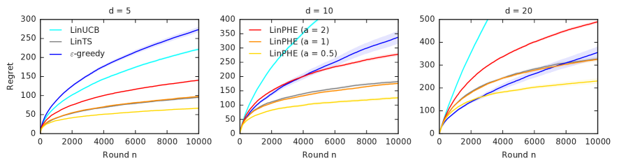
Figure 1: Comparison of ${\tt LinPHE}$ to several baselines in three linear bandit problems. All results are averaged over $100$ random problem instances. The shaded areas are standard errors of the estimates. The legend is split between the first two plots.

We conduct two experiments to evaluate both ${\tt LinPHE}$ and ${\tt LogPHE}$ in terms of their regret. The algorithms are compared to several state-of-the-art baselines.

5.1 Linear Bandit

The first experiment is with linear bandits. We experiment with dimensions $d$ from $5$ to $20$. The number of arms is $K=100$. To avoid biases, we randomly generate problem instances. Each instance is generated as follows. The first $d-1$ entries of feature vector $x_{i}$ are drawn from a unit $(d-2)$-sphere and the last entry is $1$. The first $d-1$ entries of parameter vector $\theta_{\ast}$ are drawn from a $(d-2)$-sphere with radius $0.5$ and the last entry is $0.5$. This construction guarantees that $x_{i}^{\top}\theta_{\ast}\in[0,1]$ for all arms $i$. The reward of arm $i$ is drawn i.i.d. from $\mathrm{Ber}(x_{i}^{\top}\theta_{\ast})$. The horizon is $n=10000$ rounds and our results are averaged over $100$ problem instances.

We compare ${\tt LinPHE}$ to ${\tt LinUCB}$ [1], ${\tt LinTS}$ [3], and the $\varepsilon$-greedy policy [30, 4] with a linear model. ${\tt LinUCB}$ is an OFU algorithm. We set the regularization parameter in ${\tt LinUCB}$ as $\lambda=1$. All other parameters are set as in Abbasi-Yadkori et al. [1]. ${\tt LinTS}$ is a posterior sampling algorithm. We set its prior to $\mathcal{N}(0,I_{d})$. The exploration rate in the $\varepsilon$-greedy policy is $\varepsilon_{t}=\min\{1,0.05/(2\sqrt{t})\}$, which results in about $5\%$ exploration. We experiment with three practical perturbation scales $a$ in ${\tt LinPHE}$: $2$, $1$, and $0.5$. We implement ${\tt LinPHE}$ with non-integer perturbation scales $a$ by replacing $B(a\,T_{i,t-1},1/2)$ in Section 3.2 with $B(\left\lceil a\,T_{i,t-1}\right\rceil,1/2)$.

Our results are reported in Figure 1. We observe the following trends. First, ${\tt LinPHE}$ outperforms ${\tt LinUCB}$ at all perturbation scales $a$. Second, ${\tt LinPHE}$ outperforms the $\varepsilon$-greedy policy at all perturbation scales $a$ in the first two problems. In the last problem, this happens only at $a\leq 1$. Finally, ${\tt LinPHE}$ performs similarly to ${\tt LinTS}$ at $a=1$ and outperforms it at $a=0.5$. However, the run time of ${\tt LinPHE}$ is less than a half of that of ${\tt LinTS}$. For instance, at $d=5$, the average run times of ${\tt LinPHE}$ and ${\tt LinTS}$ are $113$ and $273$ seconds, respectively. The increased run time of ${\tt LinTS}$ is due to posterior sampling from the multivariate normal distribution.

5.2 Logistic Bandit

The last experiment is with logistic bandits (Section 3.3). The experimental setup differs from Section 5.1 only in how $\theta_{\ast}$ is generated. The first $d-1$ entries of parameter vector $\theta_{\ast}$ are drawn from a $(d-2)$-sphere with radius $1.5$ and the last entry is $0$. By design, $\left|x_{i}^{\top}\theta_{\ast}\right|\leq 1.5$.

We compare ${\tt LogPHE}$ to ${\tt LogTS}$ [6, 29], ${\tt GLM\mathchar 45\relax UCB}$ [11], ${\tt UCB\mathchar 45\relax GLM}$ [21], and the $\varepsilon$-greedy policy [30, 4] with a logistic model. ${\tt GLM\mathchar 45\relax UCB}$ and ${\tt UCB\mathchar 45\relax GLM}$ are OFU methods for logistic bandits. We implement them with regularization (Section 3.3) and $\lambda=1$. The minimum derivative of the mean function, which is tunable in both methods, is set to the most optimistic value of $1/4$. All other parameters are set as suggested by theory. ${\tt LogTS}$ is a posterior sampling algorithm for logistic regression, which uses the Laplace approximation and has prior $\mathcal{N}(0,I_{d})$. The $\varepsilon$-greedy policy is implemented as in Section 5.1.

Our results are reported in Figure 2. We observe similar trends to Section 5.1. In particular, ${\tt LogPHE}$ usually outperforms OFU algorithms and is competitive with posterior sampling when $a\leq 1$. In summary, our experimental results show that both ${\tt LinPHE}$ and ${\tt LogPHE}$ perform well, and are comparable to or better than existing algorithms.

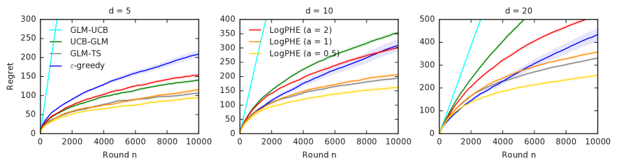
Figure 2: Comparison of ${\tt LogPHE}$ to several baselines in three logistic bandit problems. All results are averaged over $100$ random problem instances. The shaded areas are standard errors of the estimates. The legend is split between the first two plots.

6 RELATED WORK

Our work is motivated by Kveton et al. [17], who proposed a multi-armed bandit algorithm that pulls the arm with the highest average reward in its perturbed history with i.i.d. pseudo-rewards. We generalize this approach to linear, and more generally contextual, bandits. This generalization is important. While the perturbed history is conceptually simple, it is unclear how to extend it to structured problems, and assessing if such a generalization is sound is non-trivial. We propose one generalization, and show it to be both sound and effective.

Our work is related to posterior sampling. In particular, let $\mu\sim\mathcal{N}(\mu_{0},\sigma^{2})$ and $(Y_{\ell})_{\ell=1}^{s}\sim\mathcal{N}(\mu,\sigma^{2})$ be $s$ i.i.d. noisy observations of $\mu$. Then the posterior distribution of $\mu$ conditioned on $(Y_{\ell})_{\ell=1}^{s}$ is

$$\mathcal{N}\left(\frac{\mu_{0}+\sum_{\ell=1}^{s}Y_{\ell}}{s+1},\,\frac{\sigma^{2}}{s+1}\right)\,.$$ (9)

It is easy to see that the above distribution can be indirectly sampled from as follows. First, draw $s+1$ i.i.d. samples $(Z_{\ell})_{\ell=0}^{s}\sim\mathcal{N}(0,\sigma^{2})$. Then

$$\frac{\mu_{0}+\sum_{\ell=1}^{s}Y_{\ell}+\sum_{\ell=0}^{s}Z_{\ell}}{s+1}$$

is a sample from (9). This equivalence can be generalized to linear models with Gaussian noise [24]. Unfortunately, it holds only for normal random variables. Therefore, it cannot justify our perturbation scheme as a form of posterior sampling.

The design of ${\tt LinPHE}$ is similar to follow the perturbed leader (FPL) [13, 15]. FPL has been traditionally studied in the non-stochastic full-information setting. Neu and Bartok [25] extended it to semi-bandits using geometric resampling. Their algorithm cannot solve our problem efficiently because it is for a $K$-armed bandit with independent arms.

Our work is closely related to bootstrapping exploration [5, 9, 26, 31, 10, 18, 34], where the learning agent perturbs its history of observations by resampling in order to achieve exploration. Contextual bootstrapping algorithms [31, 10, 18, 34] have superior empirical performance but no regret bounds. Our work provides a stepping stone for the analysis of such algorithms, since our perturbation scheme is similar but simpler.

7 CONCLUSIONS

We propose ${\tt LinPHE}$, a new online algorithm for cumulative regret minimization in stochastic linear bandits. The key idea in ${\tt LinPHE}$ is to perturb the history in round $t$ by $O(t)$ i.i.d. pseudo-rewards, which are drawn from the maximum variance distribution. We derive a $\tilde{O}(d\sqrt{n})$ bound on the $n$-round regret of ${\tt LinPHE}$, where $d$ is the number of features. We also propose ${\tt LogPHE}$, a natural generalization of ${\tt LinPHE}$ to a logistic model. We evaluate ${\tt LinPHE}$ and ${\tt LogPHE}$ empirically. Both algorithms are competitive with Thompson sampling, although they are derived based on different insights.

${\tt LinPHE}$ can be easily extended to any linear model with a bounded support. In particular, if $Y_{i,t}\in[m,M]$, $Y_{\ell}$ in ${\tt LinPHE}$ should be replaced with $(Y_{\ell}-m)/(M-m)$.

Our work can be extended in several directions. First, although we propose ${\tt LogPHE}$ for a logistic model, we do not analyze it. We believe that the regret analysis is possible because generalized linear bandit analyses [11, 21] are similar to linear bandit analyses [7, 1]. Second, the theory-suggested perturbation scale $a$ in Table 1 is too conservative to be practical, for the same reason as the analyzed variant of ${\tt LinTS}$ in Agrawal and Goyal [3]. A tighter analysis should be possible. Third, our key technical lemmas, Lemmas 6 and 7, can be extended to other randomized pseudo-rewards than Bernoulli. This would be necessary for other generalized linear models than logistic. Finally, our design seems conservative since the strategy for adding pseudo-rewards does not adapt over time. More adaptive designs may be possible.

Appendix A PROOFS

A.1 Proof of Lemma 2

Let

$$\bar{S}_{t}=\left\{i\in[K]:(c_{1}+c_{2})\|x_{i}\|_{G_{t}^{-1}}\geq\Delta_{i}\right\}$$ (10)

be the set of undersampled arms in round $t$. Note that by definition $1\in\bar{S}_{t}$. The set of sufficiently sampled arms is defined as $S_{t}=[K]\setminus\bar{S}_{t}$. Let

$$\textstyle J_{t}=\operatorname*{arg\,min\,}_{i\in\bar{S}_{t}}\|x_{i}\|_{G_{t}^{-1}}$$ (11)

be the least uncertain undersampled arm in round $t$. In all steps below, we assume that event $E_{1,t}$ occurs.

Let $c=c_{1}+c_{2}$. In round $t$ on event $E_{2,t}$,

$$\Delta_{I_{t}}={} \Delta_{J_{t}}+\langle x_{J_{t}}^{\top}\theta_{\ast}-x_{I_{t}}^{\top}\theta_{\ast}\rangle$$

$$\leq{} \Delta_{J_{t}}+\langle x_{J_{t}}^{\top}\tilde{\theta}_{t}-x_{I_{t}}^{\top}\tilde{\theta}_{t}\rangle+{}$$

$$c\,(\langle\|x_{I_{t}}\|_{G_{t}^{-1}}\rangle+\langle\|x_{J_{t}}\|_{G_{t}^{-1}}\rangle)$$

$$\leq{} c\,(\langle\|x_{I_{t}}\|_{G_{t}^{-1}}\rangle+2\langle\|x_{J_{t}}\|_{G_{t}^{-1}}\rangle)\,,$$

where the first inequality is by the definitions of events $E_{1,t}$ and $E_{2,t}$, and the second follows from the definitions of $I_{t}$ and $J_{t}$. We also used that $c=c_{1}+c_{2}\geq 1$. Now we take the expectation of both sides and get

$$\mathbb{E}_{t}\left[\Delta_{I_{t}}\right]$$

$$\quad=\mathbb{E}_{t}\left[\Delta_{I_{t}}\mathds{1}\!\left\{E_{2,t}\right\}\right]+\mathbb{E}_{t}\left[\Delta_{I_{t}}\mathds{1}\!\left\{\bar{E}_{2,t}\right\}\right]$$

$$\quad\leq c\,\mathbb{E}_{t}\left[\langle\|x_{I_{t}}\|_{G_{t}^{-1}}\rangle+2\langle\|x_{J_{t}}\|_{G_{t}^{-1}}\rangle\right]+\mathbb{P}_{t}\left(\bar{E}_{2,t}\right)\,.$$

The last step is to bound $\mathbb{E}_{t}\left[\langle\|x_{J_{t}}\|_{G_{t}^{-1}}\rangle\right]$ from above. The key observation is that

$$\mathbb{E}_{t}\left[\langle\|x_{I_{t}}\|_{G_{t}^{-1}}\rangle\right]$$

$$\quad\geq\mathbb{E}_{t}\left[\langle\|x_{I_{t}}\|_{G_{t}^{-1}}\rangle\,\middle|\,I_{t}\in\bar{S}_{t}\right]\mathbb{P}_{t}\left(I_{t}\in\bar{S}_{t}\right)$$

$$\quad\geq\langle\|x_{J_{t}}\|_{G_{t}^{-1}}\rangle\,\mathbb{P}_{t}\left(I_{t}\in\bar{S}_{t}\right)\,,$$

where the last inequality is from the definition of $J_{t}$ and that $\bar{S}_{t}$ is $\mathcal{F}_{t-1}$-measurable. We rearrange the inequality and get

$$\langle\|x_{J_{t}}\|_{G_{t}^{-1}}\rangle\leq\mathbb{E}_{t}\left[\langle\|x_{I_{t}}\|_{G_{t}^{-1}}\rangle\right]\Big{/}\ \mathbb{P}_{t}\left(I_{t}\in\bar{S}_{t}\right)\,.$$

Next we bound $\mathbb{P}_{t}\left(I_{t}\in\bar{S}_{t}\right)$ from below. On event $E_{1,t}$,

$$\mathbb{P}_{t}\left(I_{t}\in\bar{S}_{t}\right) \geq\mathbb{P}_{t}\left(\exists i\in\bar{S}_{t}:x_{i}^{\top}\tilde{\theta}_{t}>\max_{j\in S_{t}}x_{j}^{\top}\tilde{\theta}_{t}\right)$$

$$\geq\mathbb{P}_{t}\left(x_{1}^{\top}\tilde{\theta}_{t}>\max_{j\in S_{t}}x_{j}^{\top}\tilde{\theta}_{t}\right)$$

$$\geq\mathbb{P}_{t}\left(x_{1}^{\top}\tilde{\theta}_{t}>\max_{j\in S_{t}}x_{j}^{\top}\tilde{\theta}_{t},\,E_{2,t}\text{ occurs}\right)$$

$$\geq{}\mathbb{P}_{t}\left(x_{1}^{\top}\tilde{\theta}_{t}>x_{1}^{\top}\theta_{\ast},\,E_{2,t}\text{ occurs}\right)$$

$$\geq\mathbb{P}_{t}\left(x_{1}^{\top}\tilde{\theta}_{t}>x_{1}^{\top}\theta_{\ast}\right)-\mathbb{P}_{t}\left(\bar{E}_{2,t}\right)\,.$$

Note that we require a sharp inequality because $x_{i}^{\top}\tilde{\theta}_{t}\geq\max_{j\in S_{t}}x_{j}^{\top}\tilde{\theta}_{t}$ does not imply that arm $i$ is pulled. The fourth inequality holds because for any $j\in S_{t}$,

$$x_{j}^{\top}\tilde{\theta}_{t}\leq x_{j}^{\top}\theta_{\ast}+c\|x_{j}\|_{G_{t}^{-1}}<x_{j}^{\top}\theta_{\ast}+\Delta_{j}=x_{1}^{\top}\theta_{\ast}$$

on event $E_{1,t}\cap E_{2,t}$. Finally,

$$\mathbb{P}_{t}\left(x_{1}^{\top}\tilde{\theta}_{t}>x_{1}^{\top}\theta_{\ast}\right)\geq\mathbb{P}_{t}\left(x_{1}^{\top}\tilde{\theta}_{t}-x_{1}^{\top}\bar{\theta}_{t}>c_{1}\|x_{1}\|_{G_{t}^{-1}}\right)$$

on event $E_{1,t}$, because $x_{1}^{\top}\theta_{\ast}\leq x_{1}^{\top}\bar{\theta}_{t}+c_{1}\|x_{1}\|_{G_{t}^{-1}}$ holds on event $E_{1,t}$. Now we chain all inequalities and use the definitions of $p_{1}$, $p_{2}$, and $p_{3}$ to complete the proof.

A.2 Proof of Lemma 5

By the Cauchy-Schwarz inequality,

$$x_{i}^{\top}\bar{\theta}_{t}-x_{i}^{\top}\theta_{\ast} =x_{i}^{\top}G_{t}^{-\frac{1}{2}}G_{t}^{\frac{1}{2}}(\bar{\theta}_{t}-\theta_{\ast})$$

$$\leq\|\bar{\theta}_{t}-\theta_{\ast}\|_{G_{t}}\|x_{i}\|_{G_{t}^{-1}}\,.$$

Now note that the least-squares estimate $\bar{\theta}_{t}$ is computed from sub-Gaussian rewards with variance proxy $1/4$. As a result, by Theorem 2 of Abbasi-Yadkori et al. [1] for $R=1/2$, $\|\bar{\theta}_{t}-\theta_{\ast}\|_{G_{t}}\leq c_{1}$ holds jointly in all rounds $t\leq n$ with probability of at least $1-\delta$. This concludes the proof.

A.3 Proof of Lemma 6

Let

$$U =\sum_{\ell=1}^{t-1}\sum_{j=1}^{a}x^{\top}G_{t}^{-1}X_{\ell}Z_{j,\ell}\,,$$

$$\bar{U} =\sum_{\ell=1}^{t-1}\sum_{j=1}^{a}x^{\top}G_{t}^{-1}X_{\ell}\bar{Z}_{j,\ell}\,,$$

and $D=U-\bar{U}$. Then by Hoeffding’s inequality,

$$\mathbb{P}_{t}\left(\left|x^{\top}\tilde{\theta}_{t}-x^{\top}\bar{\theta}_{t}\right|\geq c\|x\|_{G_{t}^{-1}}\right)$$

$$\quad=\mathbb{P}_{t}\left(\left|D\right|\geq c\|x\|_{G_{t}^{-1}}\right)$$

$$\quad\leq 2\exp\left[-\frac{2c^{2}\|x\|_{G_{t}^{-1}}^{2}}{a\sum_{\ell=1}^{t-1}x^{\top}G_{t}^{-1}X_{\ell}X_{\ell}^{\top}G_{t}^{-1}x}\right]\,.$$

This step of the proof relies on the fact that new $Z_{j,\ell}$ are generated in each round $t$. Also note that

$$\sum_{\ell=1}^{t-1}x^{\top}G_{t}^{-1}X_{\ell}X_{\ell}^{\top}G_{t}^{-1}x$$ (12)

$$\quad\leq x^{\top}G_{t}^{-1}\left(\sum_{\ell=1}^{t-1}X_{\ell}X_{\ell}^{\top}+\lambda I_{d}\right)G_{t}^{-1}x=\|x\|_{G_{t}^{-1}}^{2}\,.$$

Our claim follows from chaining all above inequalities.

A.4 Proof of Lemma 7

Let $U$, $\bar{U}$, and $D$ be defined as in the proof of Lemma 6. Then $x^{\top}\tilde{\theta}_{t}-x^{\top}\bar{\theta}_{t}=D$. We also define events

$$F_{1} =\left\{\left|D\right|\leq c\|x\|_{G_{t}^{-1}}\right\}\,,$$

$$F_{2} =\left\{\left|D\right|\leq\sqrt{2a\log n}\|x\|_{G_{t}^{-1}}\right\}\,.$$

Since $2a\log n>c^{2}$, $F_{1}\subset F_{2}$. Then

$$\mathrm{var}\left[U\,\middle|\,\mathcal{F}_{t-1}\right]={} \mathbb{E}_{t}\left[D^{2}\mathds{1}\!\left\{F_{1}\right\}\right]+{}$$

$$\mathbb{E}_{t}\left[D^{2}\mathds{1}\!\left\{\bar{F}_{1},F_{2}\right\}\right]+{}$$

$$\mathbb{E}_{t}\left[D^{2}\mathds{1}\!\left\{\bar{F}_{2}\right\}\right]\,.$$

Now we bound each term on the right-hand side of the above equality from above. From the definition of event $F_{1}$, term $1$ is bounded as

$$\mathbb{E}_{t}\left[D^{2}\mathds{1}\!\left\{F_{1}\right\}\right]\leq c^{2}\|x\|_{G_{t}^{-1}}^{2}\,.$$

By the definition of $F_{1}$ and $F_{2}$, term $2$ is bounded as

$$\mathbb{E}_{t}\left[D^{2}\mathds{1}\!\left\{\bar{F}_{1},F_{2}\right\}\right]$$

$$\quad\leq(2a\|x\|_{G_{t}^{-1}}^{2}\log n)\,\mathbb{P}_{t}\left(\bar{F}_{1},F_{2}\text{ occur}\right)$$

$$\quad\leq(2a\|x\|_{G_{t}^{-1}}^{2}\log n)\,\mathbb{P}_{t}\left(\left|D\right|>c\|x\|_{G_{t}^{-1}}\right)\,.$$

Now we bound term $3$. First, note that

$$\left|D\right| \leq a\sum_{\ell=1}^{t-1}\left|x^{\top}G_{t}^{-1}X_{\ell}\right|$$

$$\leq a\sqrt{n}\sqrt{\sum_{\ell=1}^{t-1}x^{\top}G_{t}^{-1}X_{\ell}X_{\ell}^{\top}G_{t}^{-1}x}$$

$$\leq a\sqrt{n}\|x\|_{G_{t}^{-1}}\,,$$

where the last step follows from (12). Then, by the definition of event $F_{2}$ and Lemma 6 for $c=\sqrt{2a\log n}$,

$$\mathbb{E}_{t}\left[D^{2}\mathds{1}\!\left\{\bar{F}_{2}\right\}\right] \leq a^{2}n\|x\|_{G_{t}^{-1}}^{2}\mathbb{P}_{t}\left(\bar{F}_{2}\right)$$

$$\leq\frac{2a^{2}\|x\|_{G_{t}^{-1}}^{2}}{n^{3}}\,.$$

Finally, by the definition of $U$,

$$\mathrm{var}\left[U\,\middle|\,\mathcal{F}_{t-1}\right] =\frac{a}{4}\sum_{\ell=1}^{t-1}x^{\top}G_{t}^{-1}X_{\ell}X_{\ell}^{\top}G_{t}^{-1}x$$

$$=\frac{a}{4}\|x\|_{G_{t}^{-1}}^{2}-\frac{a}{4}\lambda x^{\top}G_{t}^{-2}x\,.$$

We bound the last term from below as follows. For any positive semi-definite matrix $M\in\mathbb{R}^{d\times d}$,

$$x^{\top}M^{2}x =\lambda_{\max}^{2}(M)\,x^{\top}\left(\lambda_{\max}^{-2}(M)M^{2}\right)x$$

$$\leq\lambda_{\max}^{2}(M)\,x^{\top}\left(\lambda_{\max}^{-1}(M)M\right)x$$

$$=\lambda_{\max}(M)\|x\|_{M}^{2}\,,$$

where the inequality follows from the fact that all eigenvalues of $\lambda_{\max}^{-2}(M)M^{2}$ are in $[0,1]$. We apply this upper bound for $M=G_{t}^{-1}$ and get that

$$\mathrm{var}\left[U\,\middle|\,\mathcal{F}_{t-1}\right] \geq\frac{a}{4}\|x\|_{G_{t}^{-1}}^{2}-\frac{a\lambda}{4\,\lambda_{\min}(G_{t})}\|x\|_{G_{t}^{-1}}^{2}$$

$$\geq\frac{a}{4}\|x\|_{G_{t}^{-1}}^{2}-\frac{a\lambda}{4\,\lambda_{\min}(G_{d+1})}\|x\|_{G_{t}^{-1}}^{2}\,,$$

where the last inequality is by $\lambda_{\min}(G_{t})\geq\lambda_{\min}(G_{d+1})$ and holds for any $t>d$.

Now we combine all above inequalities and get

$$\left[\frac{a}{4}-\frac{a\lambda}{4\,\lambda_{\min}(G_{d+1})}-c^{2}-\frac{2a^{2}}{n^{3}}\right]\|x\|_{G_{t}^{-1}}^{2}$$

$$\quad\leq(2a\|x\|_{G_{t}^{-1}}^{2}\log n)\,\mathbb{P}_{t}\left(\left|D\right|>c\|x\|_{G_{t}^{-1}}\right)\,.$$

Since $2a\log n>0$ and $\|x\|_{G_{t}^{-1}}>0$, the above inequality can be simplified as

$$\mathbb{P}_{t}\left(\left|D\right|>c\|x\|_{G_{t}^{-1}}\right)$$

$$\quad\geq\frac{1}{8\log n}(1-\lambda\lambda_{\min}^{-1}(G_{d+1})-4a^{-1}c^{2}-8an^{-3})\,.$$

Finally, we note that the distribution of $D$ is symmetric. Therefore, for any $\varepsilon>0$, $\mathbb{P}_{t}\left(\left|D\right|>\varepsilon\right)=2\mathbb{P}_{t}\left(D>\varepsilon\right)$. This completes the proof.

References

• Abbasi-Yadkori etΒ al. [2011] Yasin Abbasi-Yadkori, David Pal, and Csaba Szepesvari. Improved algorithms for linear stochastic bandits. In Advances in Neural Information Processing Systems 24, pages 2312–2320, 2011.
• Agrawal and Goyal [2013a] Shipra Agrawal and Navin Goyal. Further optimal regret bounds for Thompson sampling. In Proceedings of the 16th International Conference on Artificial Intelligence and Statistics, pages 99–107, 2013a.
• Agrawal and Goyal [2013b] Shipra Agrawal and Navin Goyal. Thompson sampling for contextual bandits with linear payoffs. In Proceedings of the 30th International Conference on Machine Learning, pages 127–135, 2013b.
• Auer etΒ al. [2002] Peter Auer, Nicolo Cesa-Bianchi, and Paul Fischer. Finite-time analysis of the multiarmed bandit problem. Machine Learning, 47:235–256, 2002.
• Baransi etΒ al. [2014] Akram Baransi, Odalric-Ambrym Maillard, and Shie Mannor. Sub-sampling for multi-armed bandits. In Proceeding of European Conference on Machine Learning and Principles and Practice of Knowledge Discovery in Databases, 2014.
• Chapelle and Li [2011] Olivier Chapelle and Lihong Li. An empirical evaluation of Thompson sampling. In Advances in Neural Information Processing Systems 24, pages 2249–2257, 2011.
• Dani etΒ al. [2008] Varsha Dani, Thomas Hayes, and Sham Kakade. Stochastic linear optimization under bandit feedback. In Proceedings of the 21st Annual Conference on Learning Theory, pages 355–366, 2008.
• Devroye [1986] Luc Devroye. Non-Uniform Random Variate Generation. Springer-Verlag, New York, NY, 1986.
• Eckles and Kaptein [2014] Dean Eckles and Maurits Kaptein. Thompson sampling with the online bootstrap. CoRR, abs/1410.4009, 2014. URL http://arxiv.org/abs/1410.4009.
• Elmachtoub etΒ al. [2017] Adam Elmachtoub, Ryan McNellis, Sechan Oh, and Marek Petrik. A practical method for solving contextual bandit problems using decision trees. In Proceedings of the 33rd Conference on Uncertainty in Artificial Intelligence, 2017.
• Filippi etΒ al. [2010] Sarah Filippi, Olivier Cappe, Aurelien Garivier, and Csaba Szepesvari. Parametric bandits: The generalized linear case. In Advances in Neural Information Processing Systems 23, pages 586–594, 2010.
• Gopalan etΒ al. [2014] Aditya Gopalan, Shie Mannor, and Yishay Mansour. Thompson sampling for complex online problems. In Proceedings of the 31st International Conference on Machine Learning, pages 100–108, 2014.
• Hannan [1957] James Hannan. Approximation to Bayes risk in repeated play. In Contributions to the Theory of Games, volumeΒ 3, pages 97–140. Princeton University Press, Princeton, NJ, 1957.
• Jun etΒ al. [2017] Kwang-Sung Jun, Aniruddha Bhargava, Robert Nowak, and Rebecca Willett. Scalable generalized linear bandits: Online computation and hashing. In Advances in Neural Information Processing Systems 30, pages 99–109, 2017.
• Kalai and Vempala [2005] Adam Kalai and Santosh Vempala. Efficient algorithms for online decision problems. Journal of Computer and System Sciences, 71(3):291–307, 2005.
• Kawale etΒ al. [2015] Jaya Kawale, Hung Bui, Branislav Kveton, Long Tran-Thanh, and Sanjay Chawla. Efficient Thompson sampling for online matrix-factorization recommendation. In Advances in Neural Information Processing Systems 28, pages 1297–1305, 2015.
• Kveton etΒ al. [2019a] Branislav Kveton, Csaba Szepesvari, Mohammad Ghavamzadeh, and Craig Boutilier. Perturbed-history exploration in stochastic multi-armed bandits. In Proceedings of the 28th International Joint Conference on Artificial Intelligence, 2019a.
• Kveton etΒ al. [2019b] Branislav Kveton, Csaba Szepesvari, Sharan Vaswani, Zheng Wen, Mohammad Ghavamzadeh, and Tor Lattimore. Garbage in, reward out: Bootstrapping exploration in multi-armed bandits. In Proceedings of the 36th International Conference on Machine Learning, pages 3601–3610, 2019b.
• Lai and Robbins [1985] T.Β L. Lai and Herbert Robbins. Asymptotically efficient adaptive allocation rules. Advances in Applied Mathematics, 6(1):4–22, 1985.
• Lattimore and Szepesvari [2019] Tor Lattimore and Csaba Szepesvari. Bandit Algorithms. Cambridge University Press, 2019.
• Li etΒ al. [2017] Lihong Li, YuΒ Lu, and Dengyong Zhou. Provably optimal algorithms for generalized linear contextual bandits. In Proceedings of the 34th International Conference on Machine Learning, pages 2071–2080, 2017.
• Lipton etΒ al. [2018] Zachary Lipton, Xiujun Li, Jianfeng Gao, Lihong Li, Faisal Ahmed, and LiΒ Deng. BBQ-networks: Efficient exploration in deep reinforcement learning for task-oriented dialogue systems. In Proceedings of the 32nd AAAI Conference on Artificial Intelligence, pages 5237–5244, 2018.
• Liu etΒ al. [2018] Bing Liu, Tong Yu, Ian Lane, and Ole Mengshoel. Customized nonlinear bandits for online response selection in neural conversation models. In Proceedings of the 32nd AAAI Conference on Artificial Intelligence, pages 5245–5252, 2018.
• Lu and Van Roy [2017] Xiuyuan Lu and Benjamin Van Roy. Ensemble sampling. In Advances in Neural Information Processing Systems 30, pages 3258–3266, 2017.
• Neu and Bartok [2013] Gergely Neu and Gabor Bartok. An efficient algorithm for learning with semi-bandit feedback. In Proceedings of the 24th International Conference on Algorithmic Learning Theory, pages 234–248, 2013.
• Osband and Van Roy [2015] Ian Osband and Benjamin Van Roy. Bootstrapped Thompson sampling and deep exploration. CoRR, abs/1507.00300, 2015. URL http://arxiv.org/abs/1507.00300.
• Riquelme etΒ al. [2018] Carlos Riquelme, George Tucker, and Jasper Snoek. Deep Bayesian bandits showdown: An empirical comparison of Bayesian deep networks for Thompson sampling. In Proceedings of the 6th International Conference on Learning Representations, 2018.
• Rusmevichientong and Tsitsiklis [2010] Paat Rusmevichientong and John Tsitsiklis. Linearly parameterized bandits. Mathematics of Operations Research, 35(2):395–411, 2010.
• Russo etΒ al. [2018] Daniel Russo, Benjamin Van Roy, Abbas Kazerouni, Ian Osband, and Zheng Wen. A tutorial on Thompson sampling. Foundations and Trends in Machine Learning, 11(1):1–96, 2018.
• Sutton and Barto [1998] Richard Sutton and Andrew Barto. Reinforcement Learning: An Introduction. MIT Press, Cambridge, MA, 1998.
• Tang etΒ al. [2015] Liang Tang, Yexi Jiang, Lei Li, Chunqiu Zeng, and Tao Li. Personalized recommendation via parameter-free contextual bandits. In Proceedings of the 38th International ACM SIGIR Conference on Research and Development in Information Retrieval, pages 323–332, 2015.
• Thompson [1933] WilliamΒ R. Thompson. On the likelihood that one unknown probability exceeds another in view of the evidence of two samples. Biometrika, 25(3-4):285–294, 1933.
• Valko etΒ al. [2014] Michal Valko, Remi Munos, Branislav Kveton, and Tomas Kocak. Spectral bandits for smooth graph functions. In Proceedings of the 31st International Conference on Machine Learning, pages 46–54, 2014.
• Vaswani etΒ al. [2018] Sharan Vaswani, Branislav Kveton, Zheng Wen, Anup Rao, Mark Schmidt, and Yasin Abbasi-Yadkori. New insights into bootstrapping for bandits. CoRR, abs/1805.09793, 2018. URL http://arxiv.org/abs/1805.09793.