Tidal disruption event rates in galaxy merger remnants

Abstract

The rate of tidal disruption events (TDEs) depends sensitively on the stellar properties of the central galactic regions. Simulations show that galaxy mergers cause gas inflows, triggering nuclear starbursts, increasing the central stellar density. Motivated by these numerical results, and by the observed over-representation of post-starburst galaxies among TDE hosts, we study the evolution of the TDE rate in high-resolution hydrodynamical simulations of a galaxy merger, in which we capture the evolution of the stellar density around the massive black holes (BHs). We apply analytical estimates of the loss-cone theory, using the stellar density profiles from simulations, to estimate the time evolution of the TDE rate. At the second pericentre, a nuclear starburst enhances the stellar density around the BH in the least massive galaxy, leading to an enhancement of the TDE rate around the secondary BH, although the magnitude and the duration of the increase depend on the stochasticity of star formation on very small scales. The central stellar density around the primary BH remains instead fairly constant, and so is its TDE rate. After the formation of the binary, the stellar density decreases, and so does the TDE rate.

1 Introduction

When a star passes sufficiently close to a massive black hole (BH), it can get accreted. For solar-type stars and BHs with mass up to $\sim$$10^{8}\,\mathrm{M}_{\odot}$, the star is not swallowed whole, but it is tidally perturbed and destroyed, with a fraction of its mass falling back on to the BH causing a bright flare, known as a tidal disruption event (TDE; Hills, 1975; Rees, 1988).

A growing body of evidence suggests that tidal disruption event are more likely to occur in host galaxies associated with recent starbursts (Arcavi et al., 2014; French et al., 2016; Stone & Metzger, 2016; Stone & van Velzen, 2016; French et al., 2017; Law-Smith et al., 2017; Graur et al., 2018): the TDE rate in these galaxies can be 30–200 times higher than in main-sequence galaxies, with galaxy mergers a possible cause for the starburst (Zabludoff et al., 1996; Yang et al., 2004, 2008; Wild et al., 2009). Stone & van Velzen (2016) advanced the hypothesis that this increase could be due to an anomalously high central stellar density, from which most TDEs are sourced, caused by the starburst. To test this hypothesis, we set ourselves in a case including a strong nuclear starburst: a galaxy merger, when gas inflows due to tidal forces and ram-pressure shocks can trigger nuclear starbursts that form a dense stellar cusp and temporarily increase the central density (Mihos & Hernquist, 1996; Van Wassenhove et al., 2014; Capelo & Dotti, 2017; Stone et al., 2018). Van Wassenhove et al. (2014) find an enhancement of almost two orders of magnitude of the density within 10 pc around the secondary BH of a 1:4 merger, during the 150 Myr following the starburst. This suggests that, during the merger, the TDE rate can increase by a few orders of magnitude.

2 A lower limit for the tidal disruption event rate

In this section, we perform an approximate calculation to understand what are the physical parameters affecting the TDE rate $\Gamma$, defined as the number of disruptions per galaxy per unit time. In practice, for the rest of this work, we estimate the TDE rate with a more elaborated method detailed in §3.3.

Stars of mass $m_{\star}$ and radius $R_{\star}$ are disrupted if the pericentre distance to the BH, of mass $M_{\bullet}$, is smaller than the tidal disruption radius $r_{\mathrm{t}}\sim{(M_{\bullet}/m_{\star})}^{1/3}R_{\star}$. This defines a “loss cone” (Lightman & Shapiro, 1977) in angular momentum of size $L_{\mathrm{lc}}^{2}/L_{\mathrm{c}}^{2}(E)$, where $L_{\mathrm{lc}}=\sqrt{2GM_{\bullet}r_{\mathrm{t}}}$ is the maximal angular momentum per unit mass for disruption, $G$ the gravitational constant, $L_{\mathrm{c}}(E)$ is the circular (maximal) angular momentum per unit mass of an orbit, with energy per unit mass $E=v^{2}/2+\Phi(r)$, $\Phi(r)$ is the gravitational potential, and $r$ and $v$ are, respectively, the distance to the BH and relative speed.

It is customary to define two regions, whose contributions to the flux of stars match at the critical radius $r_{\mathrm{c}}$, with the corresponding specific energy $E_{\mathrm{c}}=\Phi({r_{\mathrm{c}}})$ (Syer & Ulmer, 1999). The first is a region close to the BH ($E<E_{\mathrm{c}}$, $r<r_{\mathrm{c}}$), where the time to diffuse across the loss cone is longer than the orbital period. All stars inside the loss cone will be disrupted at periapsis and the loss cone is empty. Farther away from the BH ($E>E_{\mathrm{c}}$, $r>r_{\mathrm{c}}$), the time to diffuse across the loss cone is shorter than the orbital period. Stars will scatter in and out of the loss cone during the orbital motion and the loss cone is full.

In the “empty loss-cone” region, the TDE flux (events per unit time per unit energy), depends only logarithmically on the size of the loss cone and it is given by (e.g. Magorrian & Tremaine, 1999; Wang & Merritt, 2004):

$$\mathcal{F}_{\mathrm{empty}}(E)=\frac{\mu N(E)}{\ln(L_{\mathrm{c}}^{2}/L_{\mathrm{lc}}^{2})}\sim\frac{N(E)}{T_{r}\ln(L_{\mathrm{c}}^{2}/L_{\mathrm{lc}}^{2})}\,,$$ (1)

where $N$ is the energy density function, $N(E)=4\pi^{2}L_{\mathrm{c}}^{2}f(E)P(E)$ for an ergodic phase-space distribution function $f(r,v)~{}=~{}f(E)$ (e.g Merritt, 2013); $\mu$ is the orbit-averaged diffusion coefficient in angular momentum (see Eq. (13c) in Vasiliev, 2017) and $T_{r}$ is the relaxation timescale (Spitzer & Harm, 1958).

Farther away from the BH, in the “full loss-cone” region, the TDE flux depends linearly on the size of the loss cone and it is given by:

$$\mathcal{F}_{\mathrm{full}}(E)=\frac{N(E)}{P(E)}\frac{L_{\mathrm{lc}}^{2}}{L_{\mathrm{c}}^{2}},$$ (2)

where $P$ is the radial period.

The total TDE rate $\Gamma$ is the integral over these two fluxes:

$$\Gamma=\int\!\!\mathcal{F}(E)\mathrm{d}E\sim\int_{-\infty}^{E_{\mathrm{c}}}\mathcal{F}_{\mathrm{empty}}(E)\mathrm{d}E+\int_{E_{\mathrm{c}}}^{\infty}\mathcal{F}_{\mathrm{full}}(E)\mathrm{d}E\,,$$ (3)

where $E_{c}$ is defined such that $\mathcal{F}_{\mathrm{empty}}(E_{\mathrm{c}})=\mathcal{F}_{\mathrm{full}}(E_{\mathrm{c}})$. To carefully estimate the TDE rate, one should compute the two integrals. However, in practice, the density profile close to the BH is unknown and in this work we consider only the region outside the critical radius. Therefore, we estimate a lower limit to the TDE rate, considering only the full loss-cone regime:

$$\Gamma_{\mathrm{full}}=4\pi^{2}L_{\mathrm{lc}}^{2}\int_{E_{\mathrm{c}}}^{\infty}\mathrm{d}Ef(E)=\pi L_{\mathrm{lc}}^{2}m_{\star}^{-1}\rho(r_{\mathrm{c}})\langle{v}^{-1}\rangle(r_{\mathrm{c}})\,,$$ (4)

where $\rho$ is the stellar density and $\langle v^{-1}\rangle(r)~{}=~{}m_{\star}\rho^{-1}(r)\int f(r,v)v^{-1}\,\mathrm{d}^{3}\vec{v}$. If we set $\langle{v}^{-1}\rangle\sim\sqrt{2/\pi}/\sigma$, with $\sigma=\sqrt{\langle v^{2}\rangle/3}$ being the velocity dispersion, we have:

$$\Gamma_{\textrm{full}}\sim{} 5.0\times 10^{-4}\,\mathrm{yr}^{-1}\times$$ (5)

$${\left(\frac{M_{\bullet}/m_{\star}}{10^{6}}\right)}^{4/3}\frac{R_{\star}}{\,\mathrm{R}_{\odot}}\frac{\rho(r_{\mathrm{c}})}{10^{6}\,\mathrm{M}_{\odot}\,\mathrm{pc}^{-3}}\frac{100\,\mathrm{km\ s}^{-1}}{\sigma(r_{\mathrm{c}})}.$$

We can obtain $r_{\mathrm{c}}$ by equating the full and empty loss-cone fluxes, this yields:

$$\frac{GM(r_{\mathrm{c}})}{\sigma^{2}(r_{\mathrm{c}})}\sim\frac{4\sqrt{2}}{3\pi}\,{\left(\frac{M_{\bullet}}{m_{\star}}\right)}^{4/3}R_{\star},$$ (6)

where we have assumed that the enclosed stellar mass within $r$, $M(r)$, equals $4\pi\rho(r)r^{3}/3$. To get a step further, we assume that ${\sigma^{2}(r)\sim G(M_{\bullet}+M(r))/r}$, and that $M(r_{\mathrm{c}})\sim M_{\bullet}$. Note that this last assumption is not necessarily true, but happens to give excellent results in our case (see §3.3). This yields:

$$r_{\mathrm{c}}\sim 3\,\mathrm{pc}\,{\left(\frac{M_{\bullet}/m_{\star}}{10^{6}}\right)}^{4/3}\,{\left(\frac{R_{\star}}{\,\mathrm{R}_{\odot}}\right)}\,.$$ (7)

During a galaxy merger, $\rho(r_{\mathrm{c}})$ can change by orders of magnitude (Van Wassenhove et al., 2014), while there is only moderate change in $M_{\bullet}$ and $\sigma$ (and, consequently, $r_{\mathrm{c}}$). Therefore, our limit to the TDE rate depends, almost exclusively, on the density at the radius $r_{\mathrm{c}}$, which depends only on the BH mass, for stars with similar mass and radius. This calculation is presented to understand the physical parameters impacting the TDE rate. We describe the method we use to estimate $\Gamma$ in §3.3.

3 Simulations

Similarly to Pfister et al. (2017), we perform a zoom re-simulation of the 1:4 coplanar, prograde–prograde galaxy merger from Capelo et al. (2015), which was shown to have a strong burst of nuclear star formation (see also Van Wassenhove et al., 2014), and is adopted here as a reference merger to highlight the various physical processes responsible for the evolution of the nucleus. Similar bursts were also observed in mergers with mass ratio 1:2 (coplanar and inclined orbital configurations), whereas lower mass-ratio mergers had weaker (1:6 case) or negligible (1:10) nuclear starbursts. Initially BH1, with a mass of $3.53\times 10^{6}\,\mathrm{M}_{\odot}$, is in the main galaxy, whereas BH2, with a mass of $0.88\times 10^{6}\,\mathrm{M}_{\odot}$, is in the secondary galaxy.

We re-simulate the merger phase (see Capelo et al., 2015), which begins at the second pericentre, at ${t\sim 1\,\mathrm{Gyr}}$, and lasts until the binary BH has formed, 300 Myr later. It is during this phase that the starburst occurs and we expect variations in the density and, consequently, in the TDE rate.

This re-simulation (Resim0) is performed with the public code Ramses (Teyssier, 2002). Ramses is an adaptive mesh refinement code in which the evolution of the gas is followed using a second-order unsplit Godunov scheme for the Euler equation. The approximate Harten–Lax–Van Leer Contact (Toro, 1997) Riemann solver with a MinMod total variation diminishing scheme to reconstruct the interpolated variables from their cell-centred values is used to compute fluxes at cell interfaces. Collisionless particles, dark matter (DM), stellar, and BH particles, are evolved using a particle-mesh solver with a cloud-in-cell (CIC) interpolation. The mass of DM particles ($m_{\mathrm{DM}}=1.1\times 10^{5}\,\mathrm{M}_{\odot}$) and stellar particles ($3.3\times 10^{3}\,\mathrm{M}_{\odot}$) is kept similar to that in Capelo et al. (2015) but we allow for better spatial resolution (down to $\Delta x=0.76\,\mathrm{pc}$), refining the mesh where $M_{\mathrm{DM}}^{\mathrm{cell}}+10M_{\rm b}^{\mathrm{cell}}\geq 8m_{\mathrm{DM}}$, where $M_{\mathrm{DM}}$ and $M_{\rm b}^{\mathrm{cell}}$ are, respectively, the mass of DM and baryons in the cell. Maximum refinement is enforced within $4\Delta x$ around the BH.

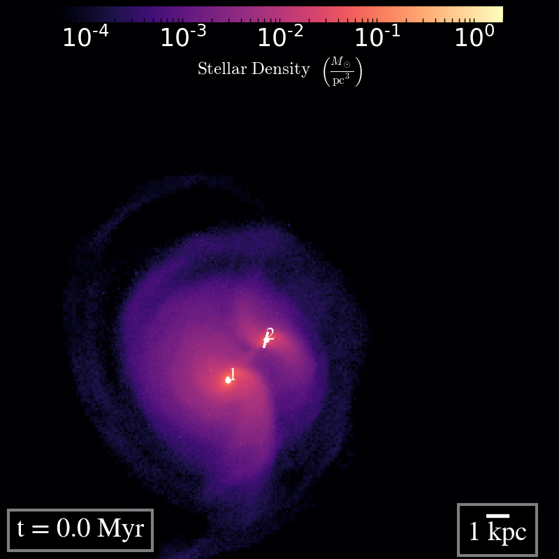
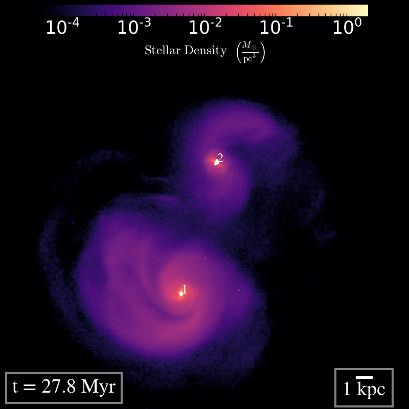
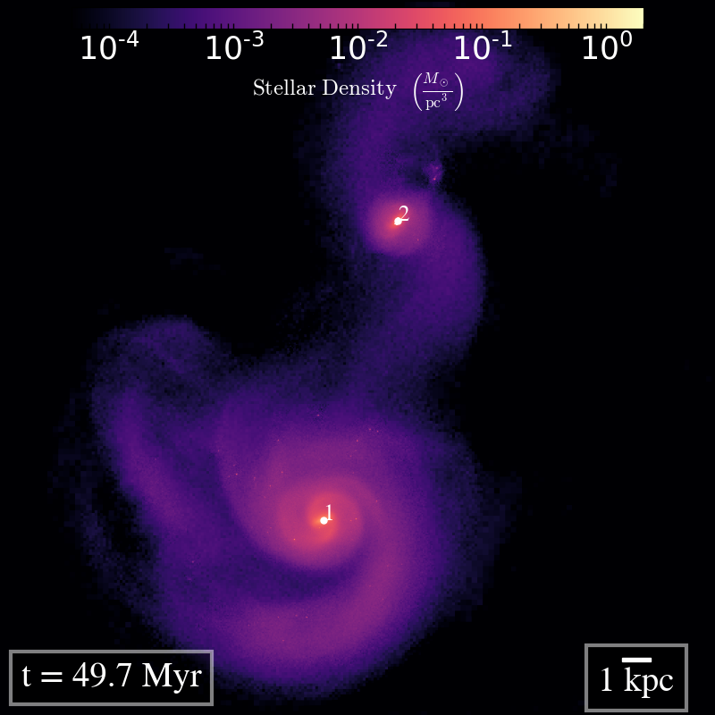
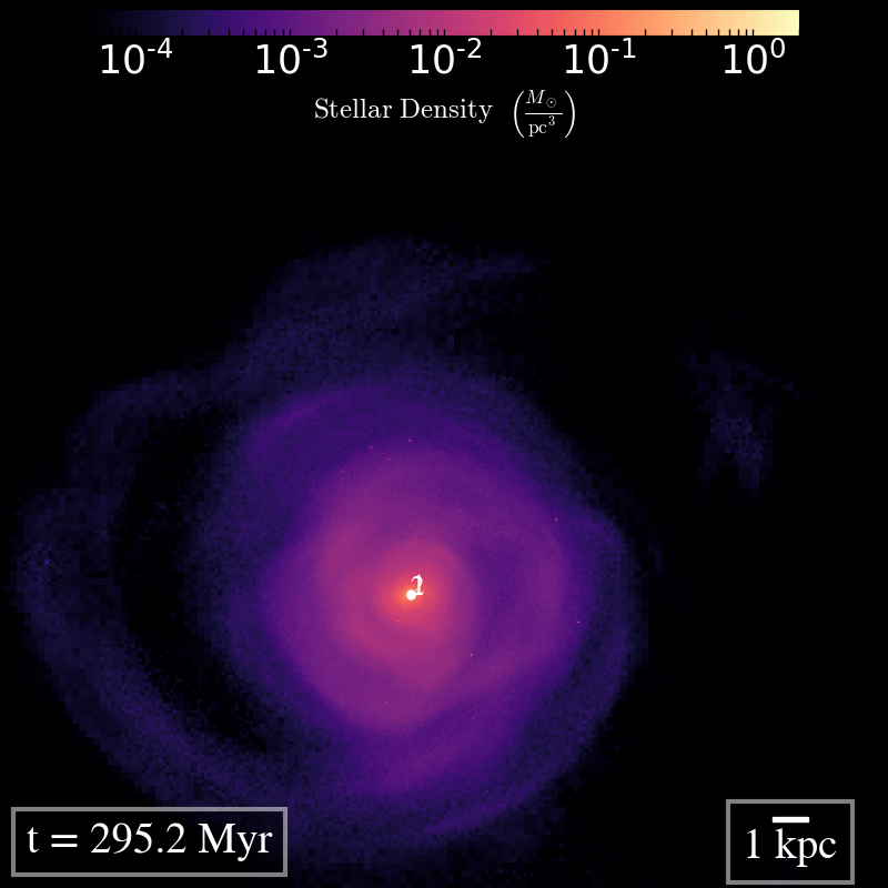
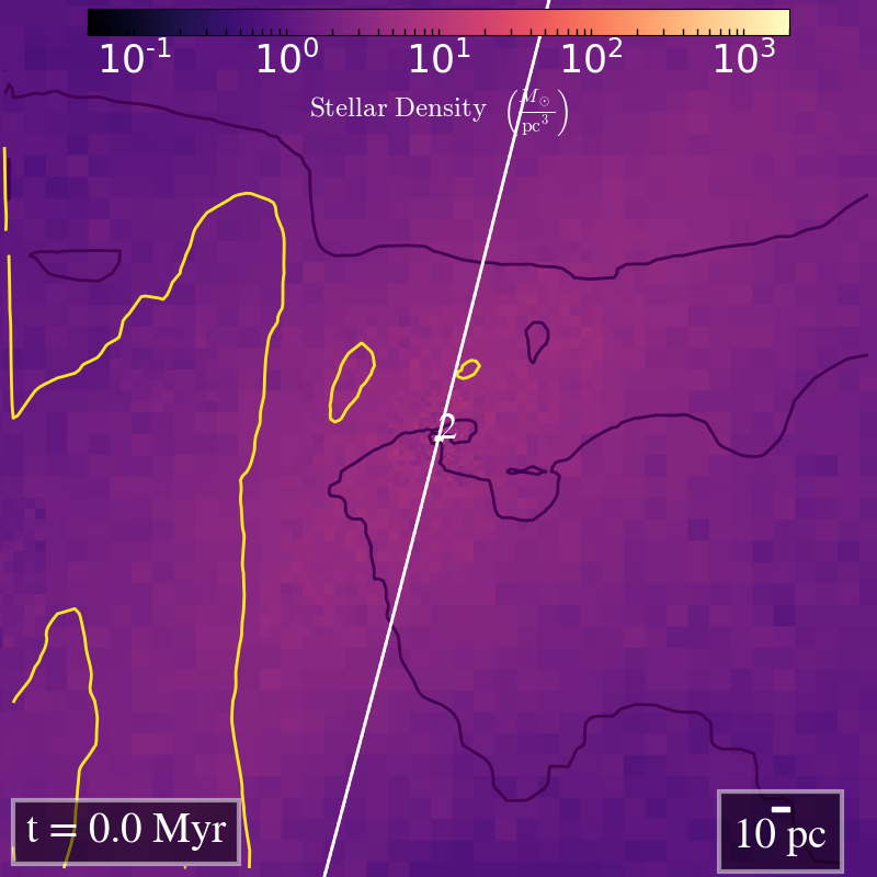
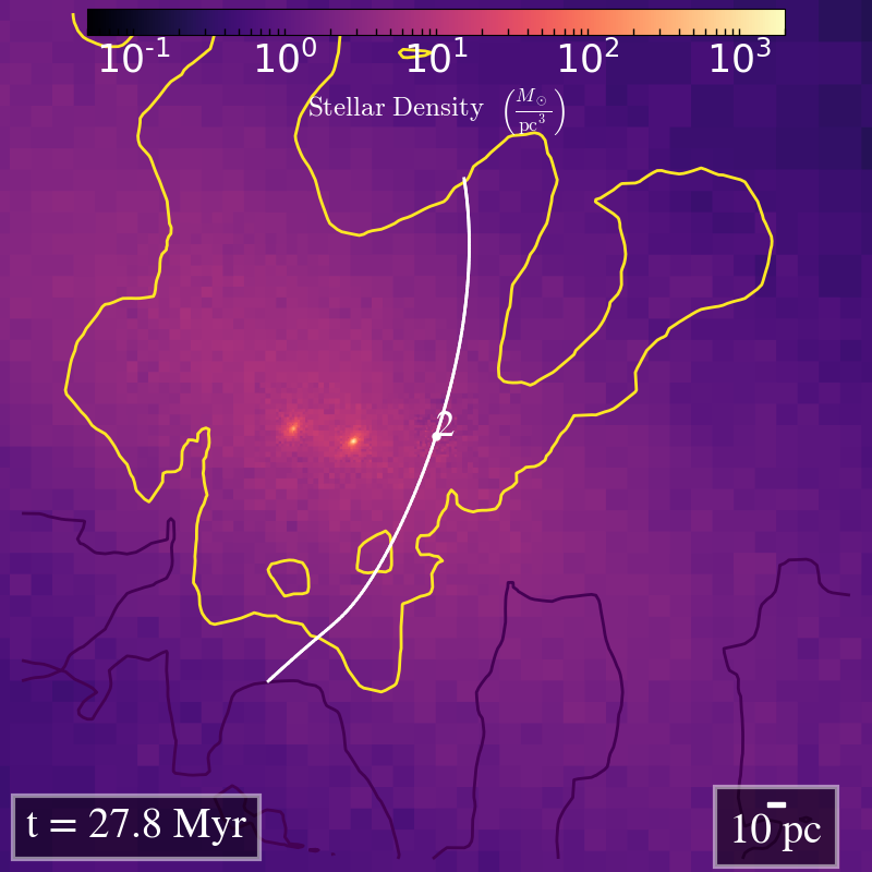
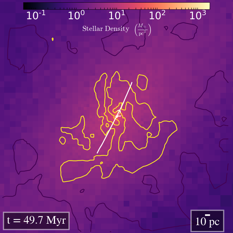
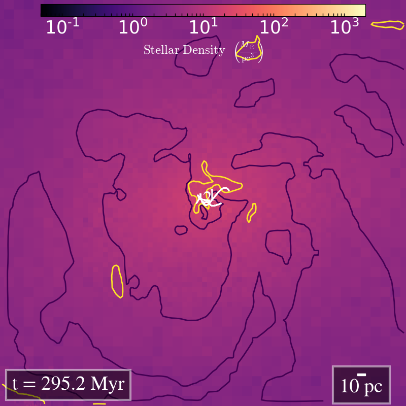
Figure 1: Stellar density maps of the two galaxies (top row) and centred on the secondary BH (bottom row). Initially, the BH proceeds on a smooth trajectory (first column); then, the starburst occurs and some newly formed stellar clumps deviate the BH from its smooth trajectory (second column); at some point, those clumps merge and the BH gets trapped (third column); finally, the BH binary forms in the remnant galaxy (fourth column). The white line in the bottom images represents the position of the BHs within $\pm 1\,\mathrm{Myr}$. In order to show how irregular is the gas density compared with the stellar one, we indicate the iso-$\rho_{\rm gas}$ contours of 1 (10) a.m.u. cm^-3 with purple (yellow) lines.

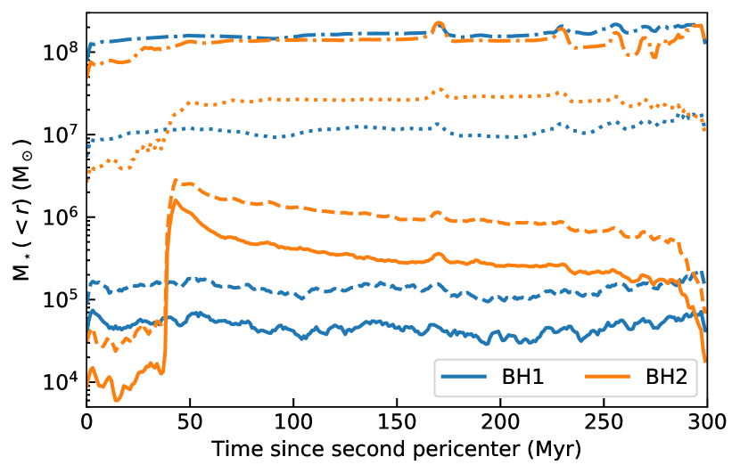
Figure 2: Enclosed stellar mass within 3 (solid), 5 (dashed), 30 (dotted), and 100 (dash-dotted) pc around each BH, as a function of time elapsed since the second pericentre.

3.1 Physics of galaxies

Gas is allowed to cool with the contribution of hydrogen, helium, and metals using tabulated cooling rates from Sutherland & Dopita (1993) above $10^{4}\,\mathrm{K}$, and rates from Rosen & Bregman (1995) below $10^{4}\,\mathrm{K}$ and down to $10\,\mathrm{K}$.

Star formation, occurring at gas densities above $1\,\rm H\,cm^{-3}$, is stochastically sampled from a random Poisson distribution (see Rasera & Teyssier 2006 for details) following a Schmidt law for the local star formation rate $\dot{\rho}=\epsilon\rho_{\rm gas}/t_{\rm ff}$, where $\rho$ and $\rho_{\rm gas}$ are the stellar and gas density, respectively, $t_{\mathrm{ff}}$ is the local gas free-fall time, and $\epsilon$ depends on the local gravo-turbulent properties of the gas, as detailed in Trebitsch et al. (2018).

For the feedback from supernovae (SNe), we use the Sedov/snowplough-aware method described in Kimm & Cen (2014), in which stars release $2\times 10^{49}\,\mathrm{erg}\,\,\mathrm{M}_{\odot}^{-1}$ after $5\,\mathrm{Myr}$ (assuming 20 per cent of the mass of star particles contributes to type II SNe).

3.2 Physics of black holes

We use the model of BHs described in Dubois et al. (2012), where accretion is computed using the Bondi–Hoyle–Lyttleton formalism capped at the Eddington luminosity. BH feedback consists of a dual-mode approach, wherein thermal energy, corresponding to 15 per cent of the bolometric luminosity (with radiative efficiency $\epsilon_{\rm r}=0.1$), is injected at high accretion rates (luminosity above 0.01 the Eddington luminosity); otherwise, feedback is modelled with a bipolar jet with a velocity of $10^{4}$ km s^-1 and an efficiency of 100 per cent.

We modify the implementation of BH dynamics. In Dubois et al. (2012), the mass of the BH is spread in a sphere of $4\Delta x$ radius around the BH in order to smooth the gravitational potential it generates. However, when two BHs approach each other, the formation of the binary is delayed. Here, we deposit all the mass of each individual BH on the particle before performing the CIC interpolation, to obtain more accurate dynamics.

3.3 TDE rate in the simulation

In Section 2, we derived Eq. (5) to get a physical insight of the relevant parameters affecting the TDE rate. In practice, however, we measure the stellar density profiles around BHs for each snapshot in our simulation and fit them with a double power-law profile $\rho(r)=\rho_{0}r^{\gamma}{(1+r/r_{0})}^{\beta-\gamma}$. We then pass these density profiles to the PhaseFlow code (included in Agama; Vasiliev 2017, 2019) which Eddington inverses them to obtain the density function $f(E)$, and compute the loss-cone filling factor $q(E)=\mu P(E)L_{\mathrm{c}}^{2}/L_{\mathrm{lc}}^{2}=\mathcal{F}_{\mathrm{empty}}/\mathcal{F}_{\mathrm{full}}\ln(L_{\mathrm{c}}/L_{\mathrm{lc}})$. The PhaseFlow code is conceived to solve the time-dependent Fokker–Planck equation, but we only use it to estimate $f$ and $q$ at each timestep corresponding to a snapshot of the simulation.

Cohn & Kulsrud (1978) estimated the instantaneous TDE flux per unit time and energy $\mathcal{F}$ (see Eq. (10–13) in Wang & Merritt (2004) or Eq. (16–17) in Stone & Metzger (2016)). We use a slightly modified version of this approximation (see Eq. (14) in Vasiliev (2017)):

$$\mathcal{F}(E)=\frac{q(E)L^{2}_{lc}/L_{c}^{2}}{(q(E)^{2}+q(E)^{4})^{1/4}+\ln(L_{c}^{2}/L_{lc}^{2})}\frac{N(E)}{P(E)}\,.$$ (8)

This expression can be integrated to obtain the TDE rate $\Gamma$. From $q$, we can also estimate the critical radius/energy solving $q(E_{c})=q(\Phi(r_{\mathrm{c}}))=\ln(L_{\mathrm{c}}/L_{\mathrm{lc}})$. Using this technique, we found that $r_{c}$ is about 20 pc at all times for BH1, and is initially 13 pc for BH2, but drops to 4–5 pc after the starburst (see §4.1). These numbers are in very good agreement with the estimates of Eq. (7): 22 and 5 pc for BH1 and BH2 (their masses are respectively $4.4\times 10^{6}\,\mathrm{M}_{\odot}$ and $1.4\times 10^{6}\,\mathrm{M}_{\odot}$, almost constant during the simulation). Consequently, for the rest of the paper, we adopt our approximate estimate of $r_{c}$.

4 Results

4.1 Nuclear starburst

In Fig. 1, we show stellar density maps of our simulation. In Fig. 2, we show the enclosed stellar mass around each BH as a function of time, for different radii in the re-simulation. It is clear from Fig. 2 that the primary galaxy is not affected by the merger: during the ${300\,\mathrm{Myr}}$ of the simulation, very few stars form around the primary BH, in agreement with the lower-resolution run (Capelo et al., 2015). Therefore, the TDE rate should remain roughly constant.

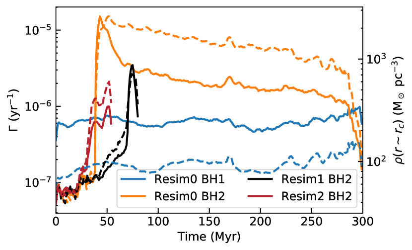
Figure 3: TDE rate around each BH (solid line) and stellar density at the critical radius (dashed line). $r_{c}$ is estimated from Eq. (7): as the masses of BH1 and BH2 are respectively $4.4\times 10^{6}$ and $1.4\times 10^{6}\,\mathrm{M}_{\odot}$, their respective $r_{c}$ are $22\,\mathrm{pc}$ and $5\,\mathrm{pc}$. We show the same quantities for BH2 in the other re-simulations (see Section 4.3), which are run for a shorter time as we are only interested in the enhancement of the stellar density following the first starburst. All quantities are shown as a function of time.

The secondary galaxy, instead, undergoes a major starburst just after the second pericentre, lasting ${50\,\mathrm{Myr}}$. As the gas is perturbed by tidal torques and ram-pressure shocks, it loses angular momentum and falls towards the centre, triggering nuclear star formation. In the original simulation from Capelo et al. (2015), this first burst is followed by other bursts similar in magnitude (see the left-hand panel of Fig. 1 in Capelo et al., 2015) that we do not see in the re-simulation. The main reason is the increase of resolution, which results in higher gas density, causing initially elevated levels of nuclear star formation, with respect to the lower-resolution run, which consume a fraction of the accumulating gas. Another difference with the original simulation from Capelo et al. (2015) is that we use a more physically motivated model for star formation, with a variable star formation efficiency: the star formation rate, therefore, is not directly proportional to the gas density. Furthermore, our much higher resolution results in clumpy star formation, as shown in the second column of Fig. 1. These clumps are fairly small (few pc size) but can be very massive, up to a few $10^{6}\,\mathrm{M}_{\odot}$, similar to the mass of BH2 ($\sim 1.4\times 10^{6}\,\mathrm{M}_{\odot}$). This leads to interactions that scatter the BH. Consequently, the density “seen” by the BH is highly dependent on local stochastic processes. The enclosed mass within ${5\,\mathrm{pc}}$ from BH2 (orange dashed line in Fig. 2) is almost constant, until it increases abruptly as the clumps merge and capture the BH at about 50 Myr. This is clear both from the third column of Fig. 1 and from Fig. 2. After this rise in density, the enclosed mass within 5 pc does not vary until the binary forms, whereas the enclosed mass within 3 pc decreases. This is contrary to the expectations of the evolution of a mass distribution around a BH, which normally contracts (Bahcall & Wolf, 1976; Quinlan et al., 1995). However, at difference with the assumptions in classic approaches, which look at equilibrium, steady-state solutions or BHs growing slowly within the stellar distribution, the BH enters rapidly the stellar clump, and the mass of the clump and the BH are similar. The effect we observe can be explained assuming that the system BH-clumps suffers a series of high-speed encounters (Binney & Tremaine, 1987), bringing enough energy to start the disruption of the clump, although we cannot rule out that the effect is numerical. When the binary forms, i.e. the BHs are separated by about 1 pc, the enclosed mass decreases again. This might be due to heating: when the binary shrinks, it releases energy in the nucleus. Since the simulation cannot resolve scatterings between stars and the binary, we are unable to rigorously confirm if this effect is physical or a numerical artifact, although detailed $N$-body simulations show similar results (e.g. Milosavljević & Merritt, 2001).

In summary, the amount of stars around BH2 changes significantly during the merger, and thus we expect large variations of its TDE rate. However, the exact enhancement may depend on the position of the BH, which can be chaotic due to three-body interactions with stellar clumps. The amount of stars around BH1 remains fairly constant and we do not expect much change in the TDE rate until it binds with BH2 and it is embedded in the same stellar environment.

4.2 TDE rate

Using the techniques described in Section 3.3, we estimate the TDE rate as a function of time in the simulations. Note that here we have taken the conservative assumption of not including an inner cusp around the BHs (Bahcall & Wolf, 1976), hence the estimated TDE rate is a lower bound.

We show in Fig. 3, as a function of time, the TDE rate around each BH (solid line) and the density at the critical radius (dashed line), as defined in Eq. (7). Note the remarkable agreement between the TDE rate measured with the PhaseFlow code and the stellar density at $r_{\mathrm{c}}$.

The initial TDE rate is very small ($\sim$$10^{-7}\,\mathrm{yr}^{-1}$ for both BHs), because the density around each BH is very low: we find, for the two BHs, a stellar density of $\sim$$10^{2}\,\mathrm{M}_{\odot}\,\,\mathrm{pc}^{-3}$, which is one to two orders of magnitude lower than in local galaxies (Faber et al., 1997). The reason is that the analytical initial conditions of the merging galaxies (Capelo et al., 2015) assume that the stellar bulge is described by a spherical Hernquist profile (Hernquist, 1990) with inner logarithmic slope $\gamma=-1$, whereas local galaxies exhibit a range of inner density slopes going from $\gamma\sim 0$ to $\gamma=-2$ (Faber et al., 1997; Lauer et al., 2007), up to $\gamma=-4$ in the presence of nuclear star clusters, common in low-mass galaxies (Glass et al., 2011). In addition, before the beginning of the merger simulation, galaxies are relaxed for ${100\,\mathrm{Myr}}$ and, during this time, the velocity distribution near the resolution limit (${10\,\mathrm{pc}}$) is not well sampled because of the limited number of stars, leading to an even shallower profile than the initial Hernquist profile.

The TDE rate around BH1 is fairly constant, irrespective of the dynamical phase of the merger: since the stellar density profile around BH1 is not affected by the merger, the amount of stars available to be disrupted is constant and so is the TDE rate. The TDE rate around BH2 is instead increased by a factor of about 30 during the $250\,\mathrm{Myr}$ following the burst, with a short peak of more than two orders of magnitude enhancement. During the first 200 Myr of this enhancement, the two galaxies can be separated by more than 1 kpc, up to 10 kpc. While the maximum value of $\sim$$10^{-5}\,\mathrm{yr}^{-1}$ may seem surprisingly low, we recall that the initial density profile, after relaxing the initial conditions, was shallow and we do not include the possibility of a stellar cusp due to unresolved stellar dynamics, which would increase the initial TDE rate and, perhaps, decrease the relative enhancement caused by merger-driven nuclear star formation.

As discussed in Section 4.1, the central density and the TDE rate drop once the binary is formed. However, to calculate the TDE rate we assumed a single BH surrounded by a spherical density distribution, which is not valid any longer after formation of the binary. More sophisticated techniques, beyond the scope of this paper, can be used for binary BHs (e.g. Lezhnin & Vasiliev, 2019), which often result in an increased rate, at least for a short time (e.g. Chen et al., 2009, 2011; Li et al., 2017).

4.3 Effect of stochasticity

We rerun the exact same simulation, but changing the random seed used in the stochastic sampling of star formation (Resim1 and Resim2), and perform the same analysis. This test is done for three main reasons: firstly, reproducibility of our results; secondly, the small number of particles around the BH in the early phase before the starburst (about $10^{4}\,\mathrm{M}_{\odot}$ within 3 pc, corresponding to 10 stellar particles; see Fig. 2) might affects our results; thirdly, because reaching pc-resolution is a double-edged sword. On the one hand, we resolve the gas flows and star formation very close to the BH. On the other hand, the stochasticity of very local processes becomes important. The exact position and mass of the forming stellar clumps have strong effects on both the orbits of BHs and on the density around them.

We show in Fig. 3 the TDE rate and density at the critical radius around BH2. In all cases, the same common trends appear: there is a starburst, which results in an enhancement of the density at the critical radius, causing an increase of the TDE rate around BH2, followed by a decay on Myr scales. However, the exact moment when the density increases, and its exact peak value, depend on the simulation, showing how small changes (the random seed and therefore the exact location of star formation) in this chaotic system can affect the TDE rate in galaxies. We note that, since the galaxy hosting BH1 is not experiencing strong star formation, the results for BH1 are the same in all three re-simulations. Overall, the mean maximal enhancement of the TDE around BH2 in the three simulations is about 140.

5 Conclusions

We assess the TDE rate around BHs using high-resolution hydrodynamical simulations of galaxies during and after a merger with mass ratio 1:4 coupled to the analytical formalism detailed in Section 2. This allows us to track the evolution of the central stellar mass during and after the merger-induced starburst, but also to measure the TDE rate in a realistic, although still idealized environment.

We summarize our findings below:

• After the first passage below $10\,\mathrm{kpc}$, a nuclear starburst promotes an enhancement of the stellar density around the BH in the least massive galaxy. As a consequence, the TDE rate also increases by up to two orders of magnitude for a short duration, and more than one order of magnitude on average.

• The nuclear starburst produces stellar clumps that scatter the BH and modulate the stellar density in its vicinity. The enhancement of the TDE rate and its duration can therefore vary significantly in different realizations of the same process.

• The environment and TDE rate around the BH in the most massive galaxy are rather unaffected by the merger.

This confirms that the TDE rate should be larger in galaxies in the final phases of mergers or the immediate post-merger phase, lasting a few hundreds of Myr, than in galaxies in isolation. However, large column densities of gas and dust concurrent with the early starbust phases (Capelo et al., 2017; Blecha et al., 2018) can hinder detection of TDEs; whereas the column density decreases in the post-merger phase allowing for easier TDE detection. This picture is independent of the stochastic behaviour of the star formation process in such a clumpy and turbulent interstellar medium. However, the exact details of the TDE enhancement, and the moment it happens, change due the small-scale turbulent dynamics (here mimicked by our perturbed re-sampling of our stochastic model for star formation), the exact set-up of the initial conditions, and additional parameters, e.g. the existence of a pre-existing cusp, or a different initial gas distribution may modulate the results. This is the first study of TDE rates using hydrodynamical simulations to track how the stellar profile is modified by star formation and external processes. We stress that this is a proof-of-concept experiment, since we have only explored one particular merger. Future work will expand to cosmological simulations.

References

- Arcavi et al. (2014) Arcavi I., et al., 2014, ApJ, 793, 38
- Bahcall & Wolf (1976) Bahcall J. N., Wolf R. A., 1976, ApJ, 209, 214
- Binney & Tremaine (1987) Binney J., Tremaine S., 1987, Galactic Dynamics, first edn. Princeton Series in Astrophysics, Princeton University Press
- Blecha et al. (2018) Blecha L., Snyder G. F., Satyapal S., Ellison S. L., 2018, MNRAS, 478, 3056
- Capelo & Dotti (2017) Capelo P. R., Dotti M., 2017, MNRAS, 465, 2643
- Capelo et al. (2015) Capelo P. R., Volonteri M., Dotti M., Bellovary J. M., Mayer L., Governato F., 2015, MNRAS, 447, 2123
- Capelo et al. (2017) Capelo P. R., Dotti M., Volonteri M., Mayer L., Bellovary J. M., Shen S., 2017, MNRAS, 469, 4437
- Chen et al. (2009) Chen X., Madau P., Sesana A., Liu F. K., 2009, ApJ, 697, L149
- Chen et al. (2011) Chen X., Sesana A., Madau P., Liu F. K., 2011, ApJ, 729, 13
- Cohn & Kulsrud (1978) Cohn H., Kulsrud R. M., 1978, ApJ, 226, 1087
- Dubois et al. (2012) Dubois Y., Devriendt J., Slyz A., Teyssier R., 2012, MNRAS, 420, 2662
- Faber et al. (1997) Faber S. M., et al., 1997, AJ, 114, 1771
- French et al. (2016) French K. D., Arcavi I., Zabludoff A., 2016, ApJ, 818, L21
- French et al. (2017) French K. D., Arcavi I., Zabludoff A., 2017, ApJ, 835, 176
- Glass et al. (2011) Glass L., et al., 2011, ApJ, 726, 31
- Graur et al. (2018) Graur O., French K. D., Zahid H. J., Guillochon J., Mandel K. S., Auchettl K., Zabludoff A. I., 2018, ApJ, 853, 39
- Hernquist (1990) Hernquist L., 1990, ApJ, 356, 359
- Hills (1975) Hills J. G., 1975, Nature, 254, 295
- Kimm & Cen (2014) Kimm T., Cen R., 2014, ApJ, 788, 121
- Lauer et al. (2007) Lauer T. R., et al., 2007, ApJ, 664, 226
- Law-Smith et al. (2017) Law-Smith J., Ramirez-Ruiz E., Ellison S. L., Foley R. J., 2017, ApJ, 850, 22
- Lezhnin & Vasiliev (2019) Lezhnin K., Vasiliev E., 2019, MNRAS, 484, 2851
- Li et al. (2017) Li S., Liu F. K., Berczik P., Spurzem R., 2017, ApJ, 834, 195
- Lightman & Shapiro (1977) Lightman A. P., Shapiro S. L., 1977, ApJ, 211, 244
- Magorrian & Tremaine (1999) Magorrian J., Tremaine S., 1999, MNRAS, 309, 447
- Merritt (2013) Merritt D., 2013, Dynamics and Evolution of Galactic Nuclei. Princeton University Press
- Mihos & Hernquist (1996) Mihos J. C., Hernquist L., 1996, ApJ, 464, 641
- Milosavljević & Merritt (2001) Milosavljević M., Merritt D., 2001, ApJ, 563, 34
- Pfister et al. (2017) Pfister H., Lupi A., Capelo P. R., Volonteri M., Bellovary J. M., Dotti M., 2017, MNRAS, 471, 3646
- Quinlan et al. (1995) Quinlan G. D., Hernquist L., Sigurdsson S., 1995, ApJ, 440, 554
- Rasera & Teyssier (2006) Rasera Y., Teyssier R., 2006, A&A, 445, 1
- Rees (1988) Rees M. J., 1988, Nature, 333, 523
- Rosen & Bregman (1995) Rosen A., Bregman J. N., 1995, ApJ, 440, 634
- Spitzer & Harm (1958) Spitzer Jr. L., Harm R., 1958, ApJ, 127, 544
- Stone & Metzger (2016) Stone N. C., Metzger B. D., 2016, MNRAS, 455, 859
- Stone & van Velzen (2016) Stone N. C., van Velzen S., 2016, ApJ, 825, L14
- Stone et al. (2018) Stone N. C., Generozov A., Vasiliev E., Metzger B. D., 2018, MNRAS, 480, 5060
- Sutherland & Dopita (1993) Sutherland R. S., Dopita M. A., 1993, ApJS, 88, 253
- Syer & Ulmer (1999) Syer D., Ulmer A., 1999, MNRAS, 306, 35
- Teyssier (2002) Teyssier R., 2002, A&A, 385, 337
- Toro (1997) Toro E. F., 1997, Riemann Solvers and Numerical Methods for Fluid Dynamics. Springer
- Trebitsch et al. (2018) Trebitsch M., Volonteri M., Dubois Y., Madau P., 2018, MNRAS, 478, 5607
- Van Wassenhove et al. (2014) Van Wassenhove S., Capelo P. R., Volonteri M., Dotti M., Bellovary J. M., Mayer L., Governato F., 2014, MNRAS, 439, 474
- Vasiliev (2017) Vasiliev E., 2017, ApJ, 848, 10
- Vasiliev (2019) Vasiliev E., 2019, MNRAS, 482, 1525
- Wang & Merritt (2004) Wang J., Merritt D., 2004, ApJ, 600, 149
- Wild et al. (2009) Wild V., Walcher C. J., Johansson P. H., Tresse L., Charlot S., Pollo A., Le Fèvre O., de Ravel L., 2009, MNRAS, 395, 144
- Yang et al. (2004) Yang Y., Zabludoff A. I., Zaritsky D., Lauer T. R., Mihos J. C., 2004, ApJ, 607, 258
- Yang et al. (2008) Yang Y., Zabludoff A. I., Zaritsky D., Mihos J. C., 2008, ApJ, 688, 945
- Zabludoff et al. (1996) Zabludoff A. I., Zaritsky D., Lin H., Tucker D., Hashimoto Y., Shectman S. A., Oemler A., Kirshner R. P., 1996, ApJ, 466, 104