A Structure Exploiting Branch-and-Bound Algorithm for Mixed-Integer Model Predictive Control

Abstract

Mixed-integer model predictive control (MI-MPC) requires the solution of a mixed-integer quadratic program (MIQP) at each sampling instant under strict timing constraints, where part of the state and control variables can only assume a discrete set of values. Several applications in automotive, aerospace and hybrid systems are practical examples of how such discrete-valued variables arise. We utilize the sequential nature and the problem structure of MI-MPC in order to provide a branch-and-bound algorithm that can exploit not only the block-sparse optimal control structure of the problem but that can also be warm started by propagating information from branch-and-bound trees and solution paths at previous time steps. We illustrate the computational performance of the proposed algorithm and compare against current state-of-the-art solvers for multiple MPC case studies, based on a preliminary implementation in Matlab and C code.

I INTRODUCTION

Optimization based control and estimation techniques, such as model predictive control (MPC) and moving horizon estimation (MHE), allow a model-based design framework in which the system dynamics and constraints can directly be taken into account [1]. This framework can be further extended to hybrid systems [2], providing a powerful technique to model a large range of problems, e.g., including dynamical systems with mode switchings or quantized control, problems with logic rules or no-go zone constraints. However, the resulting optimization problems are highly non-convex because they contain variables that only take integer values. When using a quadratic objective in combination with linear system dynamics and linear inequality constraints, the resulting optimal control problem (OCP) can be formulated as a mixed-integer quadratic program (MIQP).

We aim to solve MIQP problems of the following form:

$$\underset{X,\,U}{\text{min}}\quad \frac{1}{2}\sum_{i=0}^{N-1}x^{\top}_{i}Q_{i}x_{i}+u^{\top}_{i}R_{i}u_{i}+x^{\top}_{N}Px_{N}$$ (1a)

s.t. $$x_{0}-\hat{x}_{0}\;=\;0,$$ (1b)

$$A_{i}x_{i}+B_{i}u_{i}+a_{i}\;=\;x_{i+1},\quad i\in\{0,\ldots,N-1\},$$ (1c)

$$l^{c}_{i}\leq C_{i}x_{i}+D_{i}u_{i}\leq u^{c}_{i},\quad i\in\{0,\ldots,N-1\},$$ (1d)

$$F_{i}u_{i}\in\{0,1\},\quad i\in\{0,\ldots,N-1\},$$ (1e)

$$l^{c}_{N}\leq C_{N}x_{N}\leq u^{c}_{N},$$ (1f)

where the optimization variables are the state $X=[x_{0}^{\top},\ldots,x_{N}^{\top}]^{\top}$ and control trajectory $U=[u_{0}^{\top},\ldots,u_{N-1}^{\top}]^{\top}$. The set of constraints (1e) are binary equality constraints, since the left-hand side needs to be equal to either $0$ or $1$. For simplicity of notation, we further consider only binary control variables instead of more general integer constraints for an affine function of both state and control variables. MPC for several classes of hybrid systems can be straightforwardly formulated as in (1). Notable examples are mixed logical systems [2], where auxiliary continuous and discrete variables can be added to the input vector. Moreover, in combination with the binary constraints (1e), the affine inequalities (1d) can model various complicated but practical restrictions on the feasible region, such as no-go zones and disjoint polyhedral constraints for states and inputs.

A hybrid MPC controller aims to solve the MIQP (1) at every sampling time instant. This is a difficult task, given that mixed-integer programming is $\mathcal{NP}$-hard in general, and several methods for solving such a sequence of MIQPs have been explored in the literature. These approaches can be divided into heuristic techniques, which seek to efficiently find sub-optimal solutions to the problem, and optimization algorithms which attempt to solve the MIQPs to optimality. Examples of the former include rounding and pumping schemes [3, 4], approximate optimization algorithms [5, 6], and approximate dynamic programming [7]. The downside of fast heuristic approaches is often the lack of guarantees for finding an optimal or even an integer-feasible solution. Heuristic rounding-based approaches to mixed-integer nonlinear OCPs can be found, e.g., in [8, 9].

As for solving these problems to optimality, most of the optimization algorithms for MIQPs are based on the classical branch-and-bound (B&B) technique [10]. For the purpose of mixed-integer MPC, the standard B&B strategy has been combined with various methods for solving the relaxed convex QPs. For example, a B&B algorithm for mixed-integer MPC (MI-MPC) has been proposed in combination with a dual active-set solver in [11], with an interior point algorithm in [12], dual projected gradient methods in [13, 6], a nonnegative least squares solver in [14], and the alternating direction method of multipliers (ADMM) in [15]. Branch-and-bound methods for solving mixed-integer nonlinear OCPs have also been studied, e.g., in [16].

Another important research topic focuses on general pre-processing and modeling techniques to reduce the size and strengthen the mixed-integer problem formulations [17]. These presolve techniques are vital to the good performance of current state-of-the-art mixed-integer solvers [18], such that these methods can often solve seemingly intractable problems in practice. Lastly, the branch-and-bound method itself has been extensively studied with several improvements in branching and variable selection techniques [19, 20], including recent developments in applying machine learning techniques in order to learn “better” branching rules [21]. Finally, the branch-and-bound strategy has been generalized further, e.g., using cutting planes to tighten the convex problem relaxations, resulting in branch-and-cut or branch-and-price variants of the algorithm [10, 17]. Unlike state-of-the-art mixed-integer solvers, e.g., GUROBI [22] and MOSEK [23], our aim is to propose a tailored algorithm and its solver implementation for fast embedded MI-MPC applications, i.e., running on microprocessors with considerably less computational resources and available memory. The optimization algorithm should be relatively simple to code with a moderate use of resources, while the software implementation is preferably compact and library independent.

In this paper, our first contribution is to propose a branch-and-bound based MPC algorithm, which exploits the features of a recently proposed structure-exploiting primal active-set solver called PRESAS [24]. The latter algorithm is tailored to efficiently solve QPs with a block-sparse optimal control structure. Our second contribution is to bring various mixed-integer programming techniques, such as bound strengthening, domain propagation, and advanced branching rules, to the context of MI-MPC. In particular, we present an algorithm that exploits the sequential nature of MPC, in order to warm-start the branch-and-bound search tree and to re-use information gathered at previous time steps. A similar type of approach was proposed recently by [14], but in this work we provide not only a warm-start procedure for the integer variables but we also show how to improve the branching strategy by warm starting and how to efficiently combine this with presolving techniques for MI-MPC. Finally, the computational performance of the proposed algorithm, for a preliminary implementation in Matlab and C code, is illustrated and compared against current state-of-the-art solvers for multiple MPC case studies.

The paper is organized as follows. Section II presents the basic idea of branch-and-bound methods for mixed-integer programming. Then, Section III presents presolve techniques in the context of mixed-integer optimal control. The resulting MI-MPC algorithm and its tailored warm-starting strategies are discussed in Section IV and its performance is illustrated based on multiple numerical case studies in Section V. Finally, Section VI concludes the paper.

II MIXED-INTEGER QUADRATIC PROGRAMMING

We first introduce some of the basic concepts in mixed-integer programming based on branch-and-bound methods, such as convex relaxations and branching strategies.

II-A Convex Quadratic Program Relaxations

A standard approach to solve the MIQP (1) is to create convex relaxations of this problem (by either dropping some constraints or by re-formulating the problem and providing an approximation scheme) and then solve the relaxations in order to approach the solution to the original MIQP. A straightforward idea is to obtain convex QP relaxations by dropping the binary equality constraints (1e) and instead enforcing the affine inequality constraints $0\leq F_{i}u_{i}\leq 1$. Other convex relaxations for MIQPs have been studied in the literature such as moment or SDP relaxations that are often tighter than QP relaxations [25, 26], but they can be relatively expensive to solve for larger problems.

For the purpose of this paper, we will focus our attention on QP relaxations where we allow the binary variables to take on real values. The main reason for choosing this relaxation is that we utilize a tailored structure exploiting active-set solver, called PRESAS [24], proposed recently for efficiently solving the convex QP relaxations. The latter solver has been shown to be competitive with state-of-the-art QP solvers for embedded MPC, and it benefits strongly from warm-starting, which can be exploited when solving the sequence of QPs within the branch-and-bound strategy. Note that the relaxations need to be convex, i.e., the weight matrices $Q_{i}$, $R_{i}$ and $P$ need to be positive (semi-) definite in (1a) such that each solution to a QP relaxation is globally optimal.

II-B Branch-and-Bound Algorithm

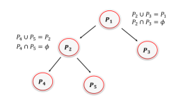
Figure 1: Illustration of the branch-and-bound method as a binary search tree. A selected node can be either branched, resulting in two partitions for each bound value in (1e), or pruned based on feasibility or the current upper bound.

The main idea of the branch-and-bound (B&B) algorithm is to sequentially create partitions of the original problem and then attempt to solve those partitions. While solving each partition may still be challenging, it is fairly efficient to obtain local lower bounds on the optimal objective value, by solving relaxations of the mixed-integer program or by using duality. If we happen to obtain an integer-feasible solution while solving a relaxation, we can then use it to obtain a global upper bound for the solution to the original problem. This may help to avoid solving or branching certain partitions that were already created, i.e., these partitions or nodes can be pruned. The general algorithmic idea of partitioning is better illustrated as a binary search tree, see Figure 1.

A key step in this approach is how to create the partitions, i.e., which node to choose and which binary variable to select for branching. Since we solve a QP relaxation at every node of the tree, it is natural to branch on one of the binary variables with fractional values in the optimal solution of the QP relaxation. Therefore, if a variable, e.g., $u_{i,k}\in\{0,1\}$ has a fractional value in a given QP relaxation, then we create two partitions where we respectively add the equality constraint $u_{i,k}=0$ and $u_{i,k}=1$. Another key step is how to choose the order in which the created subproblems are solved. These two steps have been extensively explored in the literature and various heuristics are implemented in state-of-the-art tools [19]. We provide next a brief description of strategies that we implemented in our B&B solver.

II-C Tree Search: Node Selection Strategies

A common implementation of the branch-and-bound method is based on a depth-first node selection strategy, which can be readily implemented using a last-in-first-out (LIFO) buffer. The next node to be solved is selected as one of the children of the current node and this process is repeated until a node is pruned, i.e., the node is either infeasible, optimal or dominated by the upper bound, which is followed by a backtracking procedure. Instead, a best-first strategy selects the node with the lowest local lower bound so far. In what follows, we will employ a combination of the depth-first and best-first node selection approach. This idea is motivated by aiming to find an integer-feasible solution quickly at the start of the branch-and-bound procedure (depth-first) to allow for early pruning, followed by a more greedy search for better feasible solutions (best-first).

II-D Reliability Branching for Variable Selection

The idea of reliability branching is to combine two powerful concepts for variable selection: strong branching and pseudo-costs [19]. Strong branching relies on temporarily branching, both up (to higher integer) and down (to lower integer), for every binary variable that has a fractional value in the solution of a QP relaxation in a given node, before committing to the variable that provides the highest value for a particular score function. The increase in objective values $\Delta_{i,k}^{+}$, $\Delta_{i,k}^{-}$ are computed when branching the binary variable $u_{i,k}$, respectively, up and down. Given these quantities, a simple scoring function $\text{score}(\cdot,\cdot)$ is computed for each binary variable. For instance, based on the product [20]:

$$S_{i,k}=\text{score}(\Delta_{i,k}^{-},\Delta_{i,k}^{+})=\text{max}(\Delta_{i,k}^{+},\epsilon)\,\cdot\,\text{max}(\Delta_{i,k}^{-},\epsilon),$$ (2)

given a small positive value $\epsilon>0$. This branching rule has been empirically shown to provide smaller search trees in practice [19]. The downside is that this procedure is relatively expensive since several QP relaxations are solved in order to select one variable to branch on.

The idea of pseudo-costs aims at approximating the increase of the objective function to decide which variable to branch on, without having to solve additional QP relaxations. This can be done by keeping statistic information for each binary variable, i.e., the pseudo-costs that represent the average increase in the objective value per unit change in that particular binary variable when branching. Every time that a given variable is chosen to be branched on, and the resulting relaxation is feasible, then we update each corresponding pseudo-cost with the observed increase in the objective, divided by the distance of the real to the binary value, in the form of a cumulative average. Therefore, each variable has two pseudo-costs, $\phi_{i,k}^{-}$ when the variable was branched “down” and $\phi_{i,k}^{+}$ when it was branched “up”. Given the solution to a QP relaxation, one can then use the pseudo-costs to select the binary variable with the highest score value to be branched on next:

$$S_{i,k}=\text{score}(\bar{u}_{i,k}\,\phi_{i,k}^{-},\;(1-\bar{u}_{i,k})\,\phi_{i,k}^{+}),$$ (3)

given a fractional value $\bar{u}_{i,k}$ in the QP relaxation.

This way, we select variables based on their past behavior throughout the branch-and-bound tree. However, at the beginning of the algorithm, the pseudo-costs are not yet initialized, which is when branching decisions typically impact the tree size the most. Reliability branching uses strong branching to initialize the pseudo-costs until a certain condition of reliability is satisfied, e.g., one switches to using pseudo-costs only once that particular variable has been branched on a specified number $\eta_{rel}$ of times [19]. The resulting branching rule is summarized in Algorithm 1. Note that reliability branching coincides with pseudo-cost branching if $\eta_{rel}=0$, with strong branching if $\eta_{rel}=\infty$, but typically a value $1\leq\eta_{rel}\leq 4$ is chosen.

This rule can be further augmented by implementing a look ahead limit in the number of candidates, as well as a limit in the number of iterations for each QP relaxation in the strong branching step. Note that many other branching rules exist such as, e.g., “most infeasible” branching which selects the binary variable with fractional part that is closest to $0.5$. Even though the latter rule is used quite often, e.g., in [14], it generally does not perform very well in practice [19]. Extensive empirical experiments with different branching strategies are beyond the scope of this paper.

Algorithm 1 Reliability Branching Strategy

1:$\eta_{\text{rel}}$, set C of candidate variables for branching.

2:for candidate variables $u_{i,k}$ in C do

3:     if $\#\texttt{branch}(u_{i,k})\leq\eta_{\text{rel}}$ then

4:         Strong branching on $u_{i,k}$ to compute score $S_{i,k}$.

5:         Update pseudo-costs $\phi^{-}_{i,k}$ and $\phi^{+}_{i,k}$.

6:     else

7:         $S_{i,k}=\text{score}(\bar{u}_{i,k}\,\phi_{i,k}^{-},\;(1-\bar{u}_{i,k})\,\phi_{i,k}^{+})$.

8:     end if

9:end for

10:Select variable with highest score $S^{*}=\underset{i,k}{\max}\,{S_{i,k}}$.

III PRESOLVE TECHNIQUES FOR MIXED-INTEGER OPTIMAL CONTROL

As mentioned earlier, presolve techniques are often crucial in making convex relaxations tighter such that typically fewer nodes need to be explored, sometimes to such an extent that seemingly intractable problems become tractable. Next, we briefly describe some of these concepts with a focus on domain propagation for bound strengthening and its implementation for mixed-integer optimal control.

III-A Domain Propagation for Condensed QP Subproblem

Several strengthening techniques are implemented as part of “presolve” routines in commercial solvers [18]. One particular technique that is suitable to mixed-integer optimal control is based on domain propagation, in which the goal is to strengthen bound values based on the inequality constraints (1d)-(1f) in the problem. However, the results of such a strategy are rather weak when directly applied to the block-sparse QP in (1), because the stage-wise coupling of the state variables (1c) needs to be taken into account. Therefore, we use instead the equivalent dense QP formulation in which the state variables are numerically eliminated, such that stronger bounds can be obtained for the control variables. Hence, we can use the block-structured sparsity to efficiently solve the QP relaxations, while we use the equivalent but dense format to effectively perform domain propagation.

Let us concatenate all state variables in a vector $X$ and all control variables in the vector $U$, such that Eqs. (1b)-(1c) can be written more compactly as

$$\bar{A}X=\bar{B}U+b+{E_{0}}\hat{x}_{0},$$ (4)

where we define the block-sparse matrices

$$\bar{A} =\begin{bmatrix}I&&&\\ -A_{1}&I&&\\ &\ddots&\ddots\\ &&-A_{N-1}&I\end{bmatrix},$$ (5a)

$$\bar{B} =\text{blkdiag}(B_{0},\ldots,B_{N-1})\text{ , }E_{0}=[A^{\top}_{0},0,\ldots,0]^{\top}.$$ (5b)

The matrix $\bar{A}$ is invertible such that we can write:

$$X=\bar{A}^{-1}\bar{B}U+\bar{A}^{-1}(b+{E_{0}}\hat{x}_{0}).$$ (6)

Now, we can substitute the latter expression for the state vector in OCP (1) to obtain the condensed form

$$\underset{U}{\text{min}}\quad \frac{1}{2}U^{\top}H_{\mathrm{c}}U+h_{\mathrm{c}}^{\top}U$$ (7a)

s.t. $$\bar{l}^{c}\leq D_{\mathrm{c}}U\leq\bar{u}^{c}$$ (7b)

$$F_{i}u_{i}\in\{0,1\},\quad i\in\{0,\ldots,N-1\},$$ (7c)

where the condensed matrices and vectors read as

$$H_{\mathrm{c}} =(\bar{A}^{-1}\bar{B})^{\top}Q\bar{A}^{-1}\bar{B}+R,\;D_{\mathrm{c}}=C\bar{A}^{-1}\bar{B}+D,$$ (8a)

$$h_{\mathrm{c}} =(\bar{A}^{-1}\bar{b})^{\top}Q\bar{A}^{-1}\bar{B},$$ (8b)

$$\bar{l}^{c} =l^{c}-C\bar{A}^{-1}\bar{b},\quad\bar{u}^{c}=u^{c}-C\bar{A}^{-1}\bar{b},$$ (8c)

where $\bar{b}:=b+E_{0}\hat{x}_{0}$ is defined and given $Q=\text{blkdiag}(Q_{1},\ldots,Q_{N-1},P)$ , $R=\text{blkdiag}(R_{0},\ldots,R_{N-1})$, and $l^{c}=[l^{c^{\top}}_{1},\ldots,l^{c^{\top}}_{N}]^{\top}$ and $u^{c}=[u^{c^{\top}}_{1},\ldots,u^{c^{\top}}_{N}]^{\top}$.

Given the condensed problem formulation, which can be computed offline and which is parametric in the current state value $\hat{x}_{0}$, we can then apply the following bound strengthening procedure, which is explained next for a single affine constraint $l_{b}\leq\sum_{i}d_{i}u_{i}\leq u_{b}$ in (7b). This constraint can be used to try and tighten bound values for all control variables $u_{i}$ for which $d_{i}\neq 0$, where $u_{i}$ denotes a single control variable in the vector $U$. Let $\bar{u}_{i},\underline{u}_{i}$ be the current upper/lower bounds for $u_{i}$ such that

$$d_{i}u_{i}\leq u_{b}-\sum_{j\neq i}d_{j}u_{j}\leq\underbrace{u_{b}-\sum_{j\neq i,d_{j}>0}d_{j}\underline{u}_{j}-\sum_{j\neq i,d_{j}<0}d_{j}\bar{u}_{j}}_{=:\bar{u}_{b,i}},$$ (9)

in which we divide by $d_{i}$ in order to obtain

$$u_{i}\leq\frac{\bar{u}_{b,i}}{d_{i}},\text{ if }d_{i}>0\quad\text{or}\quad u_{i}\geq\frac{\bar{u}_{b,i}}{d_{i}},\text{ if }d_{i}<0.$$ (10)

This results, respectively, in the updated bound values

$$\bar{u}_{i}=\min{(\bar{u}_{i},\frac{\bar{u}_{b,i}}{d_{i}})},\quad\text{or}\quad\underline{u}_{i}=\max{(\underline{u}_{i},\frac{\bar{u}_{b,i}}{d_{i}})},$$ (11)

or, in case $u_{i}$ is an integer or binary variable,

$$\bar{u}_{i}=\min{(\bar{u}_{i},\left\lfloor\frac{\bar{u}_{b,i}}{d_{i}}\right\rfloor)},\quad\text{or}\quad\underline{u}_{i}=\max{(\underline{u}_{i},\left\lceil\frac{\bar{u}_{b,i}}{d_{i}}\right\rceil)}.$$ (12)

where $\lfloor\cdot\rfloor$ and $\lceil\cdot\rceil$ are the floor and ceiling operations, respectively. Thus, this can result in strengthening of bound values for both continuous and integer/binary control variables. The procedure can be executed for each control variable and each inequality constraint in an iterative manner, see Algorithm 2, since bound strengthening for one variable can lead to strengthening for other variables [18]. The process is typically stopped when the bound values do not sufficiently change or a certain limit on the computation time is met.

Domain propagation can lead to considerable reductions in the amount of explored nodes, e.g., because variables are fixed, when $\bar{u}_{i}=\underline{u}_{i}$, or because of infeasibility detection, when $\bar{u}_{i}<\underline{u}_{i}$, without the need to solve any QP relaxations. In addition, the updated bound values for all control variables can be used to strengthen QP relaxations in the future. Lastly, we can use domain propagation in order to improve and generalize Hessian-based fixing strategies, such as the one proposed in [27]. Hessian-based fixing typically can only be applied to unconstrained problems, since it fixes the variables solely based on the objective. Here, we propose to use domain propagation to compute the feasibility impact of certain variable fixings. More specifically, a particular variable can be fixed based on optimality, if and only if this fixing does not induce feasibility-based fixings.

Algorithm 2 Domain Propagation for Bound Strengthening

1:Inequality constraints (7b), variable bounds $\bar{u}_{i},\underline{u}_{i}$.

2:while stopping criterion == False do

3:     for  every row of $D_{\mathrm{c}}$ do

4:         for  every $u_{i}\in U,\;d_{i}\neq 0$ do

5:              Obtain bound values $\bar{u}_{b,i},\bar{l}_{b,i}$ using Eq. (10).

6:              Update variable bounds using (11) or (12).

7:         end for

8:     end for

9:end while

10:Updated bounds $\bar{u}_{i},\underline{u}_{i}$ for all control variables.

III-B Probing Strategies and Cutting Planes

Probing [28] is a classical technique that can be incorporated in any branch-and-bound method to derive stronger inequalities or better bounds. It consists of tentatively trying to fix some variables and to derive potential logical implications on other variables. We do not further describe probing strategies in detail, but we refer to [18] for an overview. The computational cost and performance of probing can be greatly improved by relying on some of the other techniques that were discussed earlier. For example, the pseudo-costs can be used in order to choose the bound value for each binary variable that is likely to result in a low objective value. In turn, the QP relaxations that are solved in the probing procedure can be used to update the pseudo-cost values. In addition, domain propagation and other variable fixing strategies can be used to reduce the amount of QP relaxations that need to be solved.

Other presolving techniques such as cut generation can be applied using the condensed problem, and can be fully transferred to the original OCP formulation. In the present paper, we refrain from using cut generation techniques as they produce inequalities that potentially couple variables across stages. Such coupling between stages is not desirable as we rely on a block-sparsity exploiting QP solver.

III-C Resulting MIQP Algorithm for Optimal Control

Algorithm 3 describes the most important steps in our proposed B&B method for solving the MIQP in (1). It solves a block-structured QP relaxation using PRESAS [24] at every node and utilizes reliability branching (Algorithm 1) to decide the branching variables. As discussed earlier, the node selection strategy is based on a depth-first search followed by a best-first search as soon as an integer-feasible solution has been found. Note that the upper bound value UB provided to Alg. 3 can be based on an integer-feasible solution guess or it can be set to $+\infty$. Because of space limitations, the present paper will not further discuss all parameter choices in the algorithm such as, e.g., the reliability branching parameters, presolving frequency, memory usage, etc.

Algorithm 3 B&B Method for the MIQP-OCP in (1)

1:Upper bound UB, tolerance $\epsilon$.

2:LB=$-\infty$ and initialize $L=\{P_{0}\}$ with root node.

3:Select current node $P_{c}\leftarrow P_{0}$.

4:while $UB-LB>\epsilon$ do

5:     Apply domain propagation to $P_{c}$ using Alg. 2.

6:     Solve resulting QP relaxation with PRESAS.

7:     if QP is feasible and $J(\bar{X},\bar{U})\leq$ UB then

8:         if QP solution is not integer-feasible then

9:              $LB\leftarrow\min_{P\in L}{J(P)}$.

10:              Select branching variable $v$ using Alg. 1.

11:              Create subproblems $P_{u}$ “up” and $P_{l}$ “down”.

12:              Append $\{P_{l},P_{u}\}$ to $L$ if $(1-\bar{v})\phi^{+}_{v}<\bar{v}\phi^{-}_{v}$

13:              or append $\{P_{u},P_{l}\}$ to $L$, otherwise.

14:         else

15:              $UB\leftarrow J(\bar{X},\bar{U})$ and $(X^{*},U^{*})\leftarrow(\bar{X},\bar{U})$.

16:         end if

17:     end if

18:     Remove current node $P_{c}$ from to-do list in $L$.

19:     Select next node based on depth-first (last node

20:     in list $L$) or based on best lower bound.

21:end while

22:MIQP solution vector $(X^{*},U^{*})$.

IV MIXED-INTEGER MPC ALGORITHM

In embedded applications of mixed-integer MPC, one needs to solve an MIQP (1) at each sampling instant under strict timing constraints. We can leverage the fact that we solve a sequence of similar problems (parametrized by the initial condition $\hat{x}_{0}$), in order to warm-start the B&B-algorithm. We refer to our proposed warm-starting procedure as tree propagation, because the main goal is to “propagate” the B&B tree forward by one time step. We describe this process in detail below. Then, we present the resulting mixed-integer MPC algorithm.

IV-A Warm Starting based on Tree Propagation

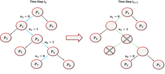
Figure 2: Illustration of the tree propagation technique from one time point to the next in the MI-MPC algorithm: index $i$ denotes the order in which each node $P_{i}$ is solved.

The warm-starting procedure aims to use knowledge of one MIQP, i.e., the search tree after solving the problem, in order to improve the B&B search for the next MIQP. Our idea is to store the path from the root to the leaf node where the optimal solution to the MIQP was found, as well as the branching order of the variables. We can then perform a shifting of this path in order to obtain a “warm-started tree” to start our search to solve the MIQP at the next time step. We illustrate this procedure in Figure 2, where the optimal path at the current time step is denoted by the sequence of nodes $P_{1}\rightarrow P_{2}\rightarrow P_{4}\rightarrow P_{6}\rightarrow P_{7}$. Let us consider a corresponding sequence of variables $u_{2}\rightarrow u_{3}\rightarrow u_{0}\rightarrow u_{1}$ that we branched on in order to create such optimal path. After shifting by one time step, all branched variables in the first control interval can be ignored, e.g., resulting in a shifted and shorter path of variables $u_{1}\rightarrow u_{2}\rightarrow u_{0}$.

At the subsequent time step, after obtaining the new state estimate, we execute all presolving techniques and we solve the QP relaxation corresponding to the root node. After removing from the warm-started tree the nodes that correspond to branched variables which are already integer feasible in the relaxed solution at the root node, we proceed by solving all the leaf nodes on the warm-started path. As we solve both children of a node on this path, we do not have to solve the parent node itself and therefore reduce computations by solving less QP relaxations. Hence, we go over the tree in the order depicted by the index of each node in Fig. 2. After the warm-started branch has been explored, we resume normal procedure of the B&B method. Algorithm 4 summarizes the proposed tree propagation technique.

Algorithm 4 Tree Propagation for Warm-Started B&B

1:Optimal path $P$ from root to leaf node.

2:Shift index of branched variables by $1$ stage along path.

3:Solve root node of shifted path $P$, including presolve.

4:for (branched variables on stage $-1$ after shifting)
   $\|$ (variables are integer feasible in root node)
   $\|$ (variables without pseudo-costs) do

5:     remove associated node from the path $P$.

6:end for

7:Shift the QP relaxation solution on every node of the path and store it as a warm start for the QP solver.

8:Re-order sequence of branched variables by scoring based on warm-started pseudo-cost information.

9:Initialize the B&B tree along the shifted path $P$, creating nodes along the path and their respective children.

10:Create the warm-started list $L$, excluding parent nodes.

11:Warm-started tree for next MIQP, given by list $L$.

The sequential nature of the problem also allows to shift and re-use the pseudo-cost information from one MPC time step to the next. This idea has the potential of producing smaller search trees as the MPC progresses, without the need to perform strong branching at every MPC step. The propagation of pseudo-costs can be coupled with an update of the reliability parameters to improve the overall performance. For example, the reliability number should be reduced for each variable from one time step to the next, in order to force strong branching for variables that have not been branched on in a sufficiently long time. In addition, nodes can be removed from the warm-started path in case they correspond to branched variables for which there is no pseudo-cost information or it is not sufficiently reliable, in an attempt to avoid bad branching decisions. Finally, these warm-started pseudo-costs can also be used to re-order the warm-started tree, in order to result in smaller search tree sizes.

The proposed tree propagation technique, with the additional re-use of pseudo-cost information, has been summarized in Algorithm 4. This procedure can improve the overall performance of the B&B method in multiple ways. First of all, the optimal path and pseudo-cost information is re-used to make better branching decisions for the mixed-integer program at the next time step, because the search trees are often similar for two subsequent problems. Also, the computational cost can be reduced by solving less QP relaxations to explore the warm-started tree. In addition, the shifted optimal path can be used in an attempt to efficiently obtain an integer-feasible solution, and therefore an important upper bound in the B&B algorithm, for the MPC problem at the next time step. Lastly, one can store the relaxed QP solutions on the optimal path, shift them by one time step and use them to warm-start the QP solver for nodes on the shifted optimal path.

IV-B MI-MPC Algorithm Implementation

Algorithm 5 summarizes the proposed MI-MPC algorithm. It solves a sequence of MIQPs where the branch-and-bound tree is warm-started at every time step, as well as the pseudo-cost and QP condensing information. As mentioned earlier, the B&B strategy and the additional presolve, warm-start and heuristic branching techniques have been implemented in Matlab, based on a C code implementation of the PRESAS algorithm [24] to solve each QP relaxation. In Section V, we illustrate the computational performance of the presented MI-MPC algorithm, including these presolving and warm-starting techniques, for two numerical case studies of mixed-integer MPC. A self-contained C code implementation is part of ongoing work, in order to illustrate the computational efficiency of the proposed algorithmic techniques.

Algorithm 5 Warm-Started B&B Algorithm for MI-MPC

1:Current state $\hat{x}_{0}$, list of nodes $L$ and pseudo-costs.

2:Solve MIQP

3:Update condensing information, given current state $\hat{x}_{0}$.

4:Formulate MIQP (1) and solve it using Algorithm 3.

5:Apply new control input $u_{0}^{\star}$ to the system.

6:Propagation Step

7:Warm-start and shift pseudo-cost information.

8:Perform tree propagation to warm-start node list $L$ for the next MI-MPC time step (see Algorithm 4).

IV-C Real-Time Embedded Applications of MI-MPC

Note that, in practice, the proposed warm-starting strategies often allow one to obtain an integer-feasible solution in a computationally efficient manner. However, even if the tree propagation immediately provides the globally optimal solution to the MIQP (1), a branch-and-bound algorithm still needs to perform relatively many iterations to prove optimality by pruning remaining nodes in the search tree. This motivates the use of a maximum number of B&B iterations in order to meet strict timing requirements of the embedded control application. Even if the algorithm does not terminate within this specified number of iterations, a feasible or even optimal solution may be available. This and other heuristic strategies for real-time implementation of MI-MPC are straightforward but outside the scope of this paper.

V CASE STUDIES: MIXED-INTEGER MPC

We report two numerical case studies to illustrate the computational performance of our MIQP-based MPC algorithm: a hybrid MPC test example and a satellite orbit re-centering application with a no-go zone in the orbital path. Our branch-and-bound algorithm has been implemented in Matlab in conjunction with the PRESAS active-set solver in C. To evaluate the performance, we compare our algorithm with the state-of-the-art GUROBI [22] and MOSEK [23] solvers for mixed-integer programming. It is important to emphasize that all advanced presolve and heuristic options have been activated for both software tools, resulting in fair computational comparisons.

V-A Hybrid MPC: Benchmark Example

The first case study is a hybrid MPC problem from [2], with the default settings as in bm99sim.m, which is a part of the Hybrid Toolbox for Matlab. This demo example has been used also more recently for numerical comparisons in [14]. The system is modeled using the HYSDEL toolbox [29] to obtain the mixed logical dynamical (MLD) system formulation. Figure 3 illustrates the average and worst-case CPU times taken by our algorithm, GUROBI and MOSEK for a range of control horizon lengths $N$.

Table I presents a detailed comparison for this test example, including additional timing results for the MI-NNLS solver that are taken directly from [14]. The latter computational results can serve only as a reference since they have been obtained on a different computer, with respect to the one used here with a 2.80 GHz Intel Xeon E3-1505M v5 processor and 32 GB of RAM. An important feature of our method is that its worst-case computation time is often rather close to the average performance in closed-loop MI-MPC simulations. This highlights the effectiveness of our tree propagation warm-starting procedure, such that consecutive branch-and-bound trees have approximately the same size. In addition, it can be observed from Table I that our proposed BB-PRESAS solver is either competitive with, or is a factor $2$ or $3$ times faster than GUROBI. The computational speedup is much larger when compared with other state-of-the-art tools such as MOSEK, our solver can be more than $10$ times faster in this particular MI-MPC test example. It shall be noted that GUROBI is a heavily optimized and fairly large software, which is unlikely to be amenable for embedded microprocessors, due to its code size, memory requirements, and software library dependencies.

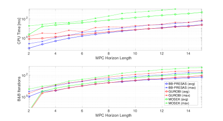
Figure 3: Computational results for closed-loop mixed-integer MPC of the bm99 example: BB-PRESAS versus GUROBI and MOSEK solvers for varying control horizon length $N$.

TABLE I: Timing results (ms) per sampling step of hybrid MPC test problem for different horizon lengths $N$. Computation times for MI-NNLS solver are taken directly from [14].

N	BB-PRESAS	GUROBI	MOSEK	MI-NNLS
	(mean/max)	(mean/max)	(mean/max)	(mean/max)
2	0.1/0.2	0.7/1.4	2.1/4.0	2.0/2.6
3	0.2/0.3	1.0/2.3	15.1/24.7	2.5/4.8
4	0.4/0.9	1.7/4.6	21.7/35.5	3.1/6.9
5	0.9/1.7	2.5/4.9	28.7/39.3	3.9/13.0
6	1.5/3.5	3.2/7.5	36.8/58.8	5.1/18.3
7	2.3/4.9	4.0/6.9	51.8/109.3	6.4/30.2
8	3.5/7.6	5.1/10.0	70.4/185.8	8.1/43.4
9	5.1/10.3	6.6/12.5	98.7/347.1	11.1/69.8
10	6.8/14.3	8.4/16.1	126.7/465.3	14.4/103.2
11	8.8/22.1	9.8/17.2	168.2/587.8	20.6/179.1
12	11.3/23.7	11.6/20.5	219.2/765.0	26.9/263.4
13	15.0/31.6	14.3/29.5	276.3/996.0	35.5/384.9
14	17.8/35.1	16.4/44.6	334.1/1241.9	46.3/562.4
15	21.0/41.6	21.9/71.6	450.8/1606.8	61.7/766.9

V-B Satellite Station Keeping with No-Go Zones

The second case study is motivated by a real-world application, namely, orbit control of a satellite in a circular low earth orbit, 400km from earth surface. The satellite propulsion system is composed of two on/off thrusters, one on each of the in-track faces of the satellite, with gimbals rotating along the vertical axis and subject to angle constraints [30]. Thus, the propulsion system is controlled by two binary and two continuous control signals. The satellite dynamics are formulated by relative motion equations (HCW) with respect to the target position along the orbit, and the cone constraints of the thrust forces are approximated as simplexes [30]. Here, we consider a re-centering maneuver in which the satellite, previously drifting, is re-centered close to the target position along the orbit. Furthermore, the error coordinates from the target position are constrained in a station keeping window ($-300\leq X\leq 300,-150\leq Y\leq 150$).

Thus, our problem is simplified from [30], by considering only the orbital dynamics in the orbital plane, i.e., ignoring the out-of-orbital-plane and attitude dynamics, and as a consequence using a simpler propulsion system with only two thrusters. To better highlight the potential of the MI-MPC method, we add an exclusion zone in the station keeping window, i.e., an area that must be avoided, which makes the allowed region of positions to be non-convex. This additional constraint is modeled using standard integer programming techniques (see, e.g., [17]), resulting in three additional binary variables for each prediction step of the mixed-integer OCP to implement the logical exclusion zone constraints. In Figure 4, we show the trajectory of the satellite in relative coordinates, where the origin is the desired satellite position along the orbit, for the simulation of the satellite controlled by the mixed-integer MPC. The depicted area in the figure corresponds to the station keeping window, in which the satellite should be kept, and the shaded area is the exclusion zone that must be avoided, at least pointwise in time. The computational timing results for this particular closed-loop MPC simulation can be found in Figure 5. One can observe that our proposed algorithm has a very competitive runtime at every MPC time step, when compared to the commercial GUROBI solver. Most importantly, the BB-PRESAS algorithm appears to perform at least as good for this particular case study in terms of worst-case computation times.

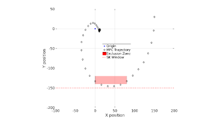
Figure 4: MPC state evolution for satellite station keeping around the origin: rectangular no-go zone is depicted in red.

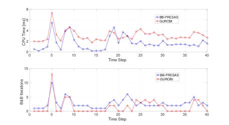
Figure 5: Closed-loop results of mixed-integer MPC for satellite station keeping: BB-PRESAS versus GUROBI solver.

VI CONCLUSIONS & OUTLOOK

In this paper, we proposed a branch-and-bound algorithm for mixed-integer MPC that exploits the optimal control problem structure to strengthen variable bounds, re-use pseudo-costs and warm-start the search tree at every MPC time step. More specifically, tailored domain propagation and tree propagation strategies have been presented. We showed preliminary results that illustrate the computational performance of our algorithm for two different MI-MPC case studies. A compact, efficient, but self-contained C code implementation of the proposed algorithm is under development to enable real-time embedded applications of hybrid MPC.

References

- [1] D. Mayne and J. Rawlings, Model Predictive Control. Nob Hill, 2013.
- [2] A. Bemporad and M. Morari, “Control of systems integrating logic, dynamics, and constraints,” Automatica, vol. 35, pp. 407–427, 1999.
- [3] T. Achterberg and T. Berthold, “Improving the feasibility pump,” Discrete Optimization, vol. 4, no. 1, pp. 77–86, 2007.
- [4] T. Achterberg, T. Berthold, and G. Hendel, “Rounding and propagation heuristics for mixed integer programming,” in Operations Research Proceedings 2011. Springer Berlin Heidelberg, 2012, pp. 71–76.
- [5] S. Diamond, R. Takapoui, and S. Boyd, “A general system for heuristic solution of convex problems over nonconvex sets,” arXiv preprint arXiv:1601.07277, 2016.
- [6] V. V. Naik and A. Bemporad, “Embedded mixed-integer quadratic optimization using accelerated dual gradient projection,” IFAC-PapersOnLine, vol. 50, no. 1, pp. 10 723–10 728, 2017.
- [7] B. Stellato, T. Geyer, and P. J. Goulart, “High-speed finite control set model predictive control for power electronics,” IEEE Transactions on Power Electronics, vol. 32, no. 5, pp. 4007–4020, May 2017.
- [8] C. Kirches, “Fast numerical methods for mixed-integer nonlinear model-predictive control,” Ph.D. dissertation, Uni. Heidelberg, 2010.
- [9] S. Sager, H. Bock, and M. Diehl, “Solving mixed-integer control problems by sum up rounding with guaranteed integer gap,” SIAM Journal on Control and Optimization, 2008.
- [10] C. A. Floudas, Nonlinear and mixed-integer optimization: fundamentals and applications. Oxford University Press, 1995.
- [11] D. Axehill and A. Hansson, “A mixed integer dual quadratic programming algorithm tailored for MPC,” in Decision and Control, 2006 45th IEEE Conference on. IEEE, 2006, pp. 5693–5698.
- [12] D. Frick, A. Domahidi, and M. Morari, “Embedded optimization for mixed logical dynamical systems,” Computers & Chemical Engineering, vol. 72, pp. 21–33, 2015.
- [13] D. Axehill and A. Hansson, “A dual gradient projection quadratic programming algorithm tailored for mixed integer predictive control.”
- [14] A. Bemporad and V. V. Naik, “A numerically robust mixed-integer quadratic programming solver for embedded hybrid model predictive control,” in Proc. 6th IFAC NMPC Conf., Madison, USA, 2018.
- [15] B. Stellato, V. Naik, A. Bemporad, and P. Goulart, “Embedded mixed-integer quadratic optimization using the OSQP solver,” in European Control Conference, 2018.
- [16] M. Gerdts, “Solving mixed-integer optimal control problems by branch&bound: a case study from automobile test-driving with gear shift,” Optimal Control Appl. and Methods, vol. 26, no. 1, pp. 1–18.
- [17] G. L. Nemhauser and L. A. Wolsey, Integer and Combinatorial Optimization. New York, NY, USA: Wiley-Interscience, 1988.
- [18] T. Achterberg, R. E. Bixby, Z. Gu, E. Rothberg, and D. Weninger, “Presolve reductions in mixed integer programming,” ZIB Report, pp. 16–44, 2016.
- [19] T. Achterberg, T. Koch, and A. Martin, “Branching rules revisited,” Operations Research Letters, vol. 33, no. 1, pp. 42–54, 2005.
- [20] P. Le Bodic and G. Nemhauser, “An abstract model for branching and its application to mixed integer programming,” Mathematical Programming, vol. 166, no. 1-2, pp. 369–405, 2017.
- [21] M.-F. Balcan, T. Dick, T. Sandholm, and E. Vitercik, “Learning to branch,” arXiv preprint arXiv:1803.10150, 2018.
- [22] L. Gurobi Optimization, “Gurobi optimizer reference manual,” ” 2018.
- [23] MOSEK ApS, The MOSEK optimization toolbox for MATLAB manual., 2017.
- [24] R. Quirynen, A. Knyazev, and S. Di Cairano, “Block structured preconditioning within an active-set method for real-time optimal control,” in Proc. European Control Conference (ECC), 2018.
- [25] Z.-Q. Luo, W.-K. Ma, A. M.-C. So, Y. Ye, and S. Zhang, “Semidefinite relaxation of quadratic optimization problems,” IEEE Signal Processing Magazine, vol. 27, no. 3, pp. 20–34, 2010.
- [26] D. Axehill, L. Vandenberghe, and A. Hansson, “Convex relaxations for mixed integer predictive control,” Automatica, vol. 46, no. 9, pp. 1540 – 1545, 2010.
- [27] D. Axehill and A. Hansson, “A preprocessing algorithm for MIQP solvers with applications to MPC,” in CDC, 2004, pp. 2497–2502.
- [28] M. W. Savelsbergh, “Preprocessing and probing techniques for mixed integer programming problems,” ORSA Journal on Computing, vol. 6, no. 4, pp. 445–454, 1994.
- [29] F. D. Torrisi and A. Bemporad, “HYSDEL-a tool for generating computational hybrid models for analysis and synthesis problems,” IEEE trans. control sys. techn., vol. 12, no. 2, pp. 235–249, 2004.
- [30] A. Walsh, S. Di Cairano, and A. Weiss, “MPC for coupled station keeping, attitude control, and momentum management of low-thrust geostationary satellites,” in ACC, July 2016, pp. 7408–7413.