Inferring Explosion Properties from Type II-Plateau Supernova Light Curves

Abstract

We present advances in modeling Type IIP supernovae using MESA for evolution to shock breakout coupled with STELLA for generating light and radial velocity curves. Explosion models and synthetic light curves can be used to translate observable properties of supernovae (such as the luminosity at day 50 and the duration of the plateau, as well as the observable quantity $ET$, defined as the time-weighted integrated luminosity that would have been generated if there was no ${\rm{}^{56}Ni}$ in the ejecta) into families of explosions which produce the same light curve and velocities on the plateau. These predicted families of explosions provide a useful guide towards modeling observed SNe, and can constrain explosion properties when coupled with other observational or theoretical constraints. For an observed supernova with a measured ${\rm{}^{56}Ni}$ mass, breaking the degeneracies within these families of explosions (ejecta mass, explosion energy, and progenitor radius) requires independent knowledge of one parameter. We expect the most common case to be a progenitor radius measurement for a nearby supernova. We show that ejecta velocities inferred from the Fe II 5169 Å line measured during the majority of the plateau phase provide little additional information about explosion characteristics. Only during the initial shock cooling phase can photospheric velocity measurements potentially aid in unraveling light curve degeneracies.

1 Introduction

Through an expanding network of ground- and space-based telescopes, the astrophysical community has an unprecedented ability to probe transient events. Along with a host of facilities, such as the All Sky Automated Survey for Supernovae (ASAS-SN; Kochanek et al. 2017), the Las Cumbres Observatory (Brown et al., 2013) is building the largest set of data ever collected on all nearby supernova (SN) events. Some SNe discovered have known progenitors in distant galaxies (Smartt, 2009). And the data are improving — The Zwicky Transient Facility (ZTF; Bellm et al. 2019) has begun discovering multiple SNe on a nightly basis, and the Large Synoptic Survey Telescope (LSST; LSST Science Collaboration et al. 2009) will revolutionize time-domain astronomy with repeated nightly imaging of the entire sky with outstanding spatial resolution.

In this paper we focus on Type IIP SNe, core-collapse events of dying massive stars ($M>10M_{\odot}$) which yield distinctive light curves that plateau over a period of $\approx$100 days. The duration and brightness of these light curves reflect the progenitor’s radius ($R$), ejected mass ($M_{\rm ej}$), energy of the explosion ($E_{\rm exp}$), and ${{}^{56}{\rm Ni}}$ mass ($M_{\rm Ni}$). Inferring these properties from the observations has broad applications. Extracting progenitor information from SN observations could lend insight into which stars explode as SNe and which collapse directly into black holes. It would also have implications for the missing red supergiant (RSG) problem identified by Smartt (2009) and updated by Smartt (2015), whereby Type II SNe with known progenitors seem to come from explosions of RSGs with initial masses of $M_{\rm ZAMS}<17M_{\odot}$, whereas evolutionary models have a cutoff mass of around $30M_{\odot}$.

Our understanding has benefitted from 3-dimensional modeling of light curves and spectroscopic data for specific Type IIP events, such as the work of Wongwathanarat et al. (2015) and Utrobin et al. (2017), as well as 3D simulations which probe specific regions of parameter space of these SNe (e.g. Burrows et al. 2019). Although 3D models are incredibly useful for describing specific systems and probing specific regions of the possible parameter space of progenitors and their explosions, substantial effort is required to estimate the parameters of a single observed explosion. The computational demand for individual 3D calculations presents a challenge for probing the parameter space of possible progenitor models for a large ensemble of explosions.

Here, we utilize the open-source 1-dimensional stellar evolution software instrument, Modules for Experiments in Stellar Astrophysics (MESA; Paxton et al. 2011, 2013, 2015, 2018, 2019), to model an ensemble of Type IIP SN progenitors, interfacing with the radiative transfer code STELLA (Blinnikov et al., 1998; Blinnikov & Sorokina, 2004; Baklanov et al., 2005; Blinnikov et al., 2006) to simulate their light curves and photospheric evolution. We include the effects of the Duffell (2016) prescription for mixing via the Rayleigh-Taylor Instability, which allows for significant mixing of important chemical species such as ${{}^{56}{\rm Ni}}$, and yields a more realistic density and temperature profile in the ejecta at shock breakout (Paxton et al. 2018, MESA IV).

The increasing abundance of data has led to a new approach to understanding Type IIP progenitors and explosions in an ensemble fashion. Pejcha & Prieto (2015b, a), and Müller et al. (2017) took such an approach, characterizing a total of 38 Type IIP SNe by their luminosity and duration of the plateau, as well as the velocity at day 50 as inferred via the Fe II 5169 Å line. By fitting these three measurements to the analytics of Popov (1993) and early numerics of Litvinova & Nadyozhin (1983), these authors inferred $M_{\rm ej}$, $E_{\rm exp}$ and $R$ from these observables.

To this end, we show that MESA+STELLA reproduces a scaling for plateau luminosity at day 50, $L_{50}$, similar to that of Popov (1993), and we introduce new best-fit scaling laws for $L_{50}$ and for the duration of the plateau $t_{\rm p}$ in the limit of ${{}^{56}{\rm Ni}}$-rich events. We also discuss the relationship between our model properties and the observable $ET$, the time-weighted integrated luminosity that would have been generated if there was no ${\rm{}^{56}Ni}$ in the ejecta (Shussman et al., 2016a; Nakar et al., 2016), and show how $ET$ can also be used to provide similar constraints on explosion properties. As an observable, $ET$ is defined by Equations (14) and (15). Additionally, we show that the measured velocity at day 50 from the Fe II 5169Å line does not scale with ejecta mass and explosion energy in the way assumed by Popov (1993). Rather, as found observationally by Hamuy (2003) and explained by Kasen & Woosley (2009), agreement in $L_{50}$ entails agreement in velocities measured near the photosphere at day 50 (as we show in Figures 21 and 22).

As our work was being completed, Dessart & Hillier (2019) submitted a paper that also highlights the non-uniqueness of light curve modeling for varied progenitor masses due to core size and mass loss due to winds. Here we additionally highlight the non-uniqueness of light curve modeling even for varied ejecta mass. As such, our calculated scaling relationships yield families of explosions with varied $R$, $M_{\rm ej}$, and $E_{\rm exp}$ which could produce comparable light curves and similar observed Fe II 5169Å line velocities (e.g. see Figures 25 and 26). Given an independent measurement of the progenitor $R$, along with a bolometric light curve and an observed nickel mass ($M_{\rm Ni}$) extracted from the tail, one can directly constrain $M_{\rm ej}$ and $E_{\rm exp}$. Otherwise, these families of explosions can be used as a starting point to guide further detailed, possibly 3D, modeling for observed events.

2 Our Models

Our modeling takes place in three steps. First, we construct a suite of core-collapse supernova progenitor models through the Si burning phase using MESA following the example_make_pre_ccsn test case, described in detail in Paxton et al. 2018 (MESA IV). Second, we load a given progenitor model at core infall, excise the core (as described in section 6.1 of MESA IV), inject energy and Ni, and evolve the model until it approaches shock breakout. This closely follows the example_ccsn_IIp test case. Third, to calculate photospheric evolution and light curves after shock breakout, we use the shock breakout profile produced in the second step as input into the public distribution of STELLA included within MESA, and run until day 175. At the end of the STELLA run, a post-processing script produces data for comparison to observational results (specifically bolometric light curves and Fe II 5169Å line velocities as described in MESA IV).

In order to create a diversity of progenitor characteristics, we chose models with variations in initial mass $M_{\rm ZAMS}$, core overshooting $f_{\rm ov}$ and $f_{\rm 0,ov}$, convective efficiency $\alpha_{\rm MLT}$ in the hydrogen envelope, wind efficiency $\eta_{\rm wind}$, modest surface rotation $\omega/\omega_{\rm crit}$, and initial metallicity $Z$. This study concerns itself especially with achieving diversity in the ejecta mass $M_{\rm ej}$ by means of the final mass at the time of explosion $M_{\rm final}$, and the radius $R$ at the time of the explosion. Table LABEL:tab:progenitors lists physical characteristics of all progenitor models utilized in this paper with $L_{\rm prog}=$ the stellar luminosity just prior to explosion. Our naming convention is determined by the ejecta mass and radius at shock breakout, M$<$$M_{\rm ej}$$>$_R$<$$R$$>$. For our sample of Type IIP SNe models, we use three progenitor models from MESA IV, the 99em_19, 99em_16, and 05cs models, renamed M16.3_R608, M12.9_R766, and M11.3_R541, respectively. Additionally, we create three new models using MESA revision 10398 to capture different regions of parameter space. We created a model with the same input parameters as 99em_19, here named M15.7_R800. In order to explore a diversity of radii for similar parameters, we also created M15.0_R1140, a model with nearly identical input to M15.7_R800, except for reduced efficiency of convective mixing $\alpha_{\rm MLT}=2.0$ (the default value is $\alpha_{\rm MLT}=3.0$) to create a more radially extended star with otherwise similar properties. Finally, in order to include smaller progenitor radii and mass in our suite, we created M9.3_R433, which has the same progenitor parameters as the 12A-like progenitor model from MESA IV, except greater overshooting $f_{\rm ov}=0.01$. These “standard suite” models are denoted by a * in Table LABEL:tab:progenitors. All models are solar metallicity, except the 05cs-like progenitor from MESA IV, M11.3_R541, which has metallicity $Z=0.006$.

Beyond this standard suite, we construct M20.8_R969, a $M_{\rm ZAMS}=25M_{\odot}$ non-rotating model with no overshooting and wind efficiency $\eta_{\rm wind}=0.4$, which has a very tightly bound core and leads to significant fallback at energies $E_{\rm exp}<2\times 10^{51}\,{\rm ergs}$ (see also Appendix A). Additionally, to highlight the families of explosions which produce comparable light curves (see Section 7), we construct three progenitor models which, when exploded with the proper explosion energy, all produce light curves similar to that of our M12.9_R766 model exploded with $0.6\times 10^{51}\,{\rm ergs}$ and $M_{\rm Ni}=0.045M_{\odot}$. M9.8_R909 was $M_{\rm ZAMS}=$13.7$M_{\odot}$ with a final mass of 11.4$M_{\odot}$, created with overshooting $f_{\rm ov}=0.016$, $f_{\rm 0,ov}=0.006$, initial rotation $(v/v_{c})_{\rm ZAMS}=0.2$, wind efficiency $\eta_{\rm wind}=1.0$, and $\alpha_{\rm MLT}=2.0$. M10.2_R848 was $M_{\rm ZAMS}=13.5M_{\odot}$ with a final mass of 12.0$M_{\odot}$, which was created with overshooting $f_{\rm ov}=0.01$, $f_{\rm 0,ov}=0.004$, initial rotation $(v/v_{c})_{\rm ZAMS}=0.2$, wind efficiency $\eta_{\rm wind}=0.8$, and $\alpha_{\rm MLT}=2.0$. M17.8_R587 was $M_{\rm ZAMS}=$20.0$M_{\odot}$ with a final mass of 19.41$M_{\odot}$, which was created with no overshooting, no rotation, wind efficiency $\eta_{\rm wind}=0.2$, and $\alpha_{\rm MLT}=3.5$.

Table 1: Properties of our RSG progenitor models at the time of the explosion. Models indicated by a * are part of our standard suite, upon which the majority of our analysis is based. $M_{\rm{c},i}$ is the mass of the excised core, and $M_{\rm He\ core}$ is the He core mass in the pre-explosion model. Names are determined by the ejecta mass and radius of each progenitor model at shock breakout, M$<$$M_{\rm ej}$$>$_R$<$$R$$>$.

model	$M_{\rm ZAMS}$	$M_{\rm final}$	$M_{\rm{c},i}$	$M_{\rm He\ core}$	$M_{\rm ej}$	$M_{\rm env}$	$\omega/\omega_{\rm crit}$	$|E_{\rm bind}|$	$T_{\rm eff}$	log($L_{\rm prog}/L_{\odot}$)	$R$
	[$M_{\odot}$]	[$M_{\odot}$]	[$M_{\odot}$]	[$M_{\odot}$]	[$M_{\odot}$]	[$M_{\odot}$]		[$10^{50}$ erg]	[K]		[$R_{\odot}$]
M9.3_R433*	11.8	10.71	1.44	3.58	9.28	7.13	0.2	1.39	4370	4.79	433
M11.3_R541*	13.0	12.86	1.57	4.22	11.29	8.65	0.0	2.65	4280	4.95	541
M12.9_R766*	16.0	14.46	1.58	5.44	12.88	9.02	0.2	4.45	3960	5.11	766
M16.3_R608*	19.0	17.79	1.51	5.72	16.29	12.07	0.2	1.29	4490	5.13	608
M15.7_R800*	19.0	17.33	1.66	6.83	15.67	10.50	0.2	2.39	4040	5.18	800
M15.0_R1140*	19.0	16.77	1.78	7.55	14.99	9.22	0.2	3.31	3660	5.32	1140
M20.8_R969	25.0	22.28	1.77	8.85	20.76	13.43	0.0	8.45	4870	5.68	969
M9.8_R909	13.7	11.36	1.60	7.75	9.8	3.61	0.2	1.81	2380	4.99	909
M10.2_R848	13.5	11.99	1.77	4.24	10.22	7.75	0.2	1.92	3510	5.13	848
M17.8_R587	20.0	19.41	1.62	7.23	17.79	12.18	0.0	2.41	5480	5.44	587

During the explosion phase, which we carry out using MESA revision 10925 to include an updated treatment of fallback (see Appendix A), we vary the total energy of the stellar model at the time of explosion ($E_{\rm tot}$) from $2\times 10^{50}$ ergs to $2\times 10^{51}\,{\rm ergs}$, with 0.2, 0.3, 0.4, 0.5, 0.6, 0.7, 0.8, 1.0, 1.2, 1.4, 1.6, and 2.0 $\times 10^{51}\,{\rm ergs}$. These models are significantly impacted by the Duffell (2016) prescription for mixing via the Rayleigh-Taylor instability, which smooths out the density profile and leads to the mixing of H deep into the interior of the ejecta and ${{}^{56}{\rm Ni}}$ out towards the outer ejecta (see MESA IV). We use the RTI coefficient $D_{\mathcal{R}}=3.0$. For a further exploration of the impact of changing the strength of RTI-driven mixing on ejecta and light curve evolution, see the work of P. Duffell et al. (2019, in preparation).

At the handoff between MESA and STELLA, we initialize STELLA with 400 zones and 40 frequency bins, and an error tolerance 0.001 for the Gear-Brayton method (Gear, 1971; Brayton et al., 1972), which leads to converged models. We also rescale the abundance profile of ${{}^{56}{\rm Ni}}$ and ${{}^{56}{\rm Co}}$ to match a specified total Nickel mass $M_{\rm Ni}$. This resets the Nickel decay clock to the time of shock breakout. We consider ${{}^{56}{\rm Ni}}$ masses of $M_{\rm Ni}/M_{\odot}=$0.0, 0.015, 0.03, 0.045, 0.06, and 0.075; the impact of ${{}^{56}{\rm Ni}}$ in our models is discussed in detail in Section 5. As most of the mixing is accounted for by Duffell RTI, we only employ modest boxcar smoothing of abundance profiles at handoff as recommended in MESA IV, using 3 boxcar passes with a width of 0.8 $M_{\odot}$. Additionally, as described in Paxton et al. 2019 and Appendix A here, we use a minimum innermost velocity cut of material moving slower than 500 km s^-1 to prevent numerical artifacts in STELLA caused during interactions between reverse shocks and slow-moving material near STELLA’s inner boundary. This study concerns itself with intrinsic properties of the SNe and their progenitors, determined primarily by quantities on the plateau, and therefore we do not include circumstellar material (CSM) in STELLA.

2.1 Estimating Fallback

Even when the total energy of a stellar model is greater than zero (i.e. the star is unbound), it is possible for some of the mass which does not collapse into the initial remnant object to become bound and fall back onto the central object, which we define as $M_{\rm fallback}$. This typically occurs as a result of inward-propagating shock waves generated at compositional boundaries within the ejecta. The relationship between progenitor binding energy, explosion energy, and fallback can be seen in Figure 1, which shows the final mass of our models versus the total energy deposited $E_{\rm dep}$, which is equal to the total energy of the model after the explosion $E_{\rm tot}$ plus the magnitude of the total energy of the bound progenitor model at the time of explosion $E_{\rm bind}$. Fallback is particularly common in explosions where the explosion energy is not significantly larger than the binding energy of the model at the time of explosion. In general, more tightly bound models require larger total final energies to unbind the entirety of the potential ejecta.

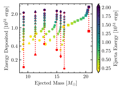
Figure 1: Energy deposited in the explosion versus ejected mass for our standard suite, as well as for the M20.8_R969 model, all exploded at 12 different explosion energies. Marker shapes correspond to different initial progenitor models as follows — pentagon: M9.3_ R433; triangle: M11.3_R541; circle: M12.9_R766; hexagon: M15.0_R1140; diamond: M15.7_R800; star: M16.3_R608; square: M20.8_R969. Explosions which would have $E_{\rm tot}=0$ (corresponding to $E_{\rm dep}=|E_{\rm bind}|$) are shown as red points whose x-coordinate is determined by the same model assuming no fallback. The red dotted line serves as a visual guide, indicating explosions with no fallback for each progenitor model. Color corresponds to the total energy of the ejecta just after the explosion $E_{\rm tot}$.

The proper treatment of fallback in 1D simulations remains an open question because of complexities such as the interaction between accretion-powered luminosity and the inner boundary of the explosion models. In MESA, the current implementation of fallback is effective as a computationally robust approximation that allows experimentation, but it should not be viewed as an accurate model of the physical processes at work. Consequently we restrict our study to models with little fallback material: $M_{\rm fallback}<0.4M_{\odot}$. The models which survive this cut are shown in figure 2. For a full description of our treatment of fallback, see Appendix A.

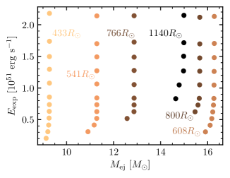
Figure 2: Ejecta masses and explosion energies as determined by the kinetic energy at day 50 in STELLA considered as a part of our standard suite, with fallback masses $M_{\rm fallback}<0.4M_{\odot}$. Lighter colors correspond to smaller progenitor radii, which are labeled.

3 Analytic Expectations

The luminosity of a Type IIP SN is, approximately, powered by shock cooling due to expansion out to around 20 days (the “shock cooling phase”), then Hydrogen recombination until around 100 days (the “plateau phase”), and the radioactive decay chain of ${{}^{56}{\rm Ni}}\rightarrow{{}^{56}{\rm Co}}\rightarrow{{}^{56}{\rm Fe}}$ beyond that (the “Nickel tail”).

The expansion time of the SN ejecta is expressed as $t_{\rm e}\approx R/v_{\rm SN}$, where $R$ is the radius of the star at the time of the explosion, and the velocity $v_{\rm SN}$ is defined by the mass of the ejecta $M_{\rm ej}$ and kinetic energy of the ejecta at infinity $E_{\rm exp}=M_{\rm ej}\,v_{\rm SN}^{2}/2$. Similarly, the time it takes to reach shock breakout after core collapse ($t_{\rm SB}$) scales with $t_{\rm e}$, such that

$$t_{\rm SB}\approx 0.91{\rm d}\ R_{500}E_{51}^{-1/2}M_{10}^{1/2},$$ (1)

where $R_{500}=R/500R_{\odot}$, $E_{51}=E_{\rm exp}/10^{51}\,{\rm ergs}$, and $M_{10}=M_{\rm ej}/10M_{\odot}$, and the dimensionful prefactor comes from a linear fit to our numerical models. This timescale is primarily a property of the models, but would observationally correspond to the difference in time between the first neutrino signal from core collapse and the first detection in the electromagnetic spectrum from shock breakout.

Following Kasen & Woosley (2009), in the limit of no accumulated heating of the ejecta due to ${{}^{56}{\rm Ni}}$ decay, the luminosity on the plateau (taken here to be at day 50, denoted $L_{50}$) is set by the total internal energy ($E$) to be radiated out divided by the duration of the plateau:

$$L_{50}=\frac{E(t_{\rm p})}{t_{\rm p}}=\frac{E_{0}t_{\rm e}}{t_{\rm p}^{2}},$$ (2)

where $t_{\rm p}$ is the duration of the plateau, $E_{0}\approx E_{\rm exp}/2$ is the initial internal energy of the ejecta at shock breakout, and the second equality comes from assuming the internal energy evolution for homologous expansion (where $r(t)\approx vt$, for a Lagrangian fluid element with constant velocity $v$) in a radiation-dominated plasma, $E_{0}t_{\rm e}=E(t_{\rm p})t_{\rm p}$.

Here we compare to the analytics of Popov (1993), which consider the effects of both H recombination and radiative diffusion. Historically, analytic scalings which ignore recombination (Arnett, 1980) or radiative diffusion (Woosley & Weaver, 1988; Chugai, 1991) have also been considered. These scalings are also detailed in Kasen & Woosley (2009) and Sukhbold et al. (2016). From a 2-zone model including an optically thick region of expanding ejecta behind the photosphere and an optically thin region outside the photosphere, Popov finds that the luminosity on the plateau (here taken at day 50) and duration of the plateau should scale as

$$\begin{split}L_{50}&\propto M^{-1/2}E_{\rm exp}^{5/6}R^{2/3}\kappa^{-1/3}T_{\rm I}^{4/3},\\ t_{0}&\propto M^{1/2}E_{\rm exp}^{-1/6}R^{1/6}\kappa^{1/6}T_{\rm I}^{-2/3},\end{split}$$ (3)

where $\kappa$ is the opacity in the optically thick component of the ejecta, and $T_{\rm I}$ is the ionization temperature of Hydrogen, and $M$ is the relevant mass (which could depend on the extent to which H is mixed throughout the ejecta). Kasen & Woosley (2009) recovers a similar set of scalings from their models:

$$\begin{split}L_{50}&\propto M_{\rm ej}^{-1/2}E_{\rm exp}^{5/6}R^{2/3}X_{\rm He}^{1},\\ t_{0}&\propto M_{\rm ej}^{1/2}E_{\rm exp}^{-1/4}R^{1/6}X_{\rm He}^{1/2},\end{split}$$ (4)

where $X_{\rm He}$ is the mass fraction of He. There is some disagreement in the literature as to whether the mass $M$ used in the Popov scalings should be the mass of the hydrogen-rich envelope ($M_{\rm env}$) or the mass of the ejecta ($M_{\rm ej}$). Sukhbold et al. (2016), for example, use $M_{\rm env}$ in recreating these scalings, since recombination in the Hydrogen-rich envelope drives the evolution of the supernova, with little contribution from the hydrogen-poor innermost ejecta coming from the core. However, in our models, the relevant mass is the total ejecta mass $M_{\rm ej}$, as we see mixing of hydrogen deep into the interior of the star and core elements into the envelope due to RTI. Since hydrogen recombination thus plays a significant role in setting the temperature throughout the entirety of the ejecta, it is the entire ejecta mass that is used in the scalings we derive later. Additionally, we make the assumption that by day 50, $E_{\rm exp}$ is equal to the kinetic energy of the ejecta.

Popov also recommended assuming that the observed photospheric velocity of the supenova ejecta should scale like $v_{\rm SN}$, such that $v_{\rm Ph}~{}\propto~{}(E_{\rm exp}/M_{\rm ej})^{1/2}$. However, this scaling, which does describe the typical velocity of the SN ejecta, should not be used when describing photospheric velocities at a fixed time, for reasons we discuss in Section 6.

The above scalings do not take into account additional heating by the radioactive decay chain of ${{}^{56}{\rm Ni}}$, which does not significantly affect the luminosity on the plateau, but does extend the duration of the plateau by heating the ejecta at late times. We discuss more detailed expectations for the effects of ${{}^{56}{\rm Ni}}$ in Appendix B, and its impact on our models in Section 5. This correction is typically written as

$$t_{\rm p}=t_{0}\times f_{\rm rad}^{1/6},$$ (5)

where $f_{\rm rad}$ can be expressed as

$$f_{\rm rad}=1+C_{f}M_{\rm Ni}\,M_{\rm ej}^{-1/2}E_{\rm exp}^{-1/2}R^{-1},$$ (6)

and $C_{f}$ is a numerical prefactor which encodes the energy and decay time of the ${{}^{56}{\rm Ni}}$ decay chain (Kasen & Woosley 2009; Sukhbold et al. 2016; and Appendix B).

These scaling relationships serve as a useful guide when modeling Type IIP supernova light curves. However, complexities arising from changes in temperature profiles, density profiles, realistic distributions of important elements such as H and ${{}^{56}{\rm Ni}}$, and stellar structure can lead to differences between these simple analytic expectations and numerical models. For example, the Popov analytics are derived for emission from a two-zone model with an optically thick inner region with a single opacity $\kappa$ and an optically thin outer region and a flat density profile. More realistic evolution of the temperature and density profiles of one of our SN ejecta models is shown in Figure 3, akin to Figure 11 of Utrobin (2007).

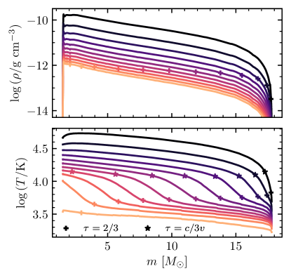
Figure 3: Density (upper panel) and temperature (lower panel) of the ejecta at every 10 days in the evolution starting at day 20 for our M16.3_R608 model exploded with $10^{51}\,{\rm ergs}$ and $M_{\rm Ni}=0.03M_{\odot}$. Darker colors indicate earlier times. Also plotted are the photosphere ($\tau=2/3$; plus markers), and the location where $\tau=c/3v$ (star markers), which is shown only on the temperature plot to reduce clutter, to demonstrate the extent of the region where the photon diffusion time is shorter than the expansion time.

Thus, in the following sections we aim to provide expressions which relate observables to the physical properties of the explosions, namely the progenitor $R$, $M_{\rm ej}$, and $E_{\rm exp}$, while also capturing the ejecta structure underlying these events.

4 Luminosity at day 50

We use the bolometric luminosity 50 days after shock breakout, $L_{50}$, as our diagnostic for the plateau luminosity, as in most cases, this is beyond the time where shock heating of CSM would affect the luminosity (Morozova et al., 2017). Moreover, for all but one progenitor model, increasing the amount of ${{}^{56}{\rm Ni}}$ has a negligible impact on $L_{50}$, as the internal energy at day 50 of the outer region of the ejecta is still dominated by the initial shock. However, in explosions where the plateau is naturally short, there can be marginal, but noticeable, additional luminosity at day 50 from ${{}^{56}{\rm Ni}}$ decay. This can be seen in Figure 4, which shows the differences between a selection of light curves and the corresponding light curves with no ${{}^{56}{\rm Ni}}$. We show light curves for M16.3_R608, a typical model with a typical $M_{\rm Ni}=0.03M_{\odot}$ (left), and for high $M_{\rm Ni}=0.075M_{\odot}$ explosions of the only progenitor model in which we see significant deviation in $L_{50}$ as a result of ${{}^{56}{\rm Ni}}$ heating, M9.3_R433 (right), where $L_{50}$ varies by up to 15% between an explosion with no ${{}^{56}{\rm Ni}}$ and one with $M_{\rm Ni}=0.075M_{\odot}$. Noting this, we choose a moderate, constant value of $M_{\rm Ni}=0.03M_{\odot}$ typical of observed events (Müller et al., 2017), and calculate how $L_{50}$ scales with $M_{\rm ej}$, $E_{\rm exp}$, and $R$.

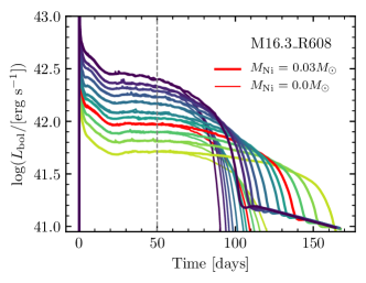
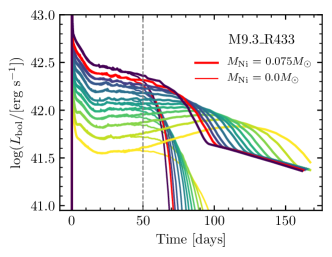
Figure 4: Light curves for increasing explosion energies of our M16.3_R608 model with $M_{\rm Ni}=0.03M_{\odot}$ (left) and our smallest model, M9.3_R433, with $M_{\rm Ni}=0.075M_{\odot}$ (right). Thin lines correspond to the same explosions, but with no ${{}^{56}{\rm Ni}}$. The red lines correspond to the models with the typical $M_{\rm Ni}$ given $L_{50}$, from the relationship in Pejcha & Prieto (2015b), and their no-nickel counterparts.

We fit two formulae to our sample suite of 57 explosions. First, we assume the power law coefficients of Popov (1993), and let the normalization float, finding

$$\begin{split}&\log(L_{50}/[{\rm erg\,s^{-1}}])=\\ &42.18-\frac{1}{2}\log M_{10}+\frac{5}{6}\log E_{51}+\frac{2}{3}\log R_{500},\end{split}$$ (7)

where $42.18$ is a linear fit from our models and logarithms are base 10, with $M_{10}=M_{\rm ej}/10M_{\odot}$, $R_{500}=R/500R_{\odot}$, and $E_{51}=E_{\rm exp}/10^{51}$ ergs. For these models, root mean square (RMS) deviations of $L_{50}$ from values derived by applying Equation (7), corresponding to the blue points in Figure 5, are $7.9\%$, with a maximum deviation in $L_{50}$ of $32\%$. The normalization for an explosion with $M_{10}=R_{500}=E_{51}=1$ is comparable to but somewhat lower than the value of 42.27 given in Sukhbold et al. (2016) (who use $M_{\rm env}$ rather than $M_{\rm ej}$), as well as the value of 42.21 calculated in Popov (1993) for default H recombination temperatures and opacities. Kasen & Woosley (2009) give a value of 42.10$+\log(X_{\rm He}/0.33)$, letting $X_{\rm He}$ range from 0.33 to 0.54.

We perform a second fit for the normalization and the power laws in $M_{10},\ E_{51},$ and $R_{500}$, and recover scalings that are similar to those in Equation (7). We find a slightly shallower scaling with $M_{\rm ej}$ and $E_{\rm exp}$, and a slightly steeper dependence on $R_{500}$:

$$\begin{split}&\log(L_{50}/[{\rm erg\,s^{-1}}])=\\ &42.16-0.40\log M_{10}+0.74\log E_{51}+0.76\log R_{500},\end{split}$$ (8)

where the normalization and power law coefficients are fit from our models. The RMS deviation of the models from Equation (8), shown as red triangles in Figure 5, is 4.7%, with deviations not exceeding 14.3% for any model with $M_{\rm Ni}=0.03M_{\odot}$. This is a better fit than the one that assumes the exact Popov scaling.

The luminosities of our models, as they compare to the fitted formulae, are shown in Figure 5. Most models agree with the Popov scaling, while the Popov scaling overpredicts $L_{50}$ in low-ejecta mass high-explosion energy cases. The x-axis of Figure 5 is $t_{\rm SB}$, chosen because it scales with explosion energy for a fixed ejecta mass and radius (Equation (1)), and increases with increasing $M_{\rm ej}$ and $R$, visually distinguishing the six different progenitor models and different explosion energies.

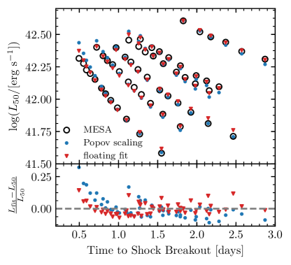
Figure 5: Fitting formulae predictions for $L_{50}$ (colored markers) compared with the model $L_{50}$ (black circles; upper panel), and their residuals (lower panel) for our suite of 57 explosions at constant $M_{\rm Ni}=0.03M_{\odot}$. Each diagonal family of points reflects one progenitor model exploded with different energies.

Although the presence of ${{}^{56}{\rm Ni}}$ does not affect light curve properties at day 50 in a majority of models, in a few explosions there is slight variation in $L_{50}$ introduced by the extra heating from ${{}^{56}{\rm Ni}}$ (seen in Figure 4). Because this effect is only distinctly noticeable in our model with the smallest values of $M_{\rm ej}$ and $R$, this can lead to variations in our recovered power laws when fitting to different fixed ${{}^{56}{\rm Ni}}$ masses. However, this correction is typically small, falling within the scatter in which our models agree with the fitted formulae. We find that the power law scalings of Equation (8) describe all models with $M_{\rm Ni}$ ranging from $0.0-0.075M_{\odot}$ within 18.2%, with RMS deviations of 4.8%, where the largest deviations occur in events where $M_{\rm Ni}=0.0M_{\odot}$, which are not consistent with any observed Type IIP SNe.

We now use Equation (8) to compare our MESA+STELLA results to models from other software instruments. In Table 2, we show our predictions for $L_{50}$ compared against luminosities from the MESA+CMFGEN models (without Duffell RTI) of Dessart et al. (2013), the Kepler+Sedona models of Kasen & Woosley (2009), and the MESA+CMFGEN models in Lisakov et al. (2017). In general, the disagreement between our formula and these other models is similar to the scatter within our own models, with the exception of the two lowest-energy explosions in Kasen & Woosley (2009) and the low luminosity suite in Lisakov et al. (2017). Equation (8) agrees with the Dessart et al. (2013) models with an RMS error of 9%, but slightly underpredicts luminosity in a majority of cases. Compared to the models of Kasen & Woosley (2009), Equation (8) gives RMS errors of 17% with no clear under- or overprediction. The low-luminosity models from Lisakov et al. (2017) have greater disagreement, with RMS errors 23% from Equation (8). This is not surprising, as on the low-luminosity end, our treatment of fallback discussed in Section 2 and Appendix A excludes most models in this region of parameter space from our fitting formulae, as significant fallback after the initial core collapse is often seen for low explosion energies.

Table 2: Comparison of Equation (8) to CMFGEN models from Dessart et al. (2013), Kepler+Sedona models from Kasen & Woosley (2009), and low-luminosity CMFGEN models from Lisakov et al. (2017). Bolometric luminosities at day 50 for Dessart et al. (2013) are recovered from light curves provided by L. Dessart (private communication). These luminosities are compared to Equation (8) applied to $M_{\rm ej}$, $E_{\rm exp}$, and $R$ from the various models.

Source	Model	$M_{\rm ej}$	$E_{\rm exp}$	$R$	$L_{50}$	Equation (8)	% diff
		[M⊙]	[$10^{51}$ erg]	[$R_{\odot}$]	[1042 erg s-1]	[1042 erg s-1]
Dessart+13	m15Mdot	10.01	1.28	776	2.55	2.40	-5%
	m15	12.48	1.27	768	2.56	2.17	-15%
	m15e0p6	12.46	0.63	768	1.19	1.29	8%
	m15mlt1	12.57	1.24	1107	3.13	2.81	-10%
	m15mlt3	12.52	1.34	501	1.61	1.63	1%
	m15os	10.28	1.40	984	3.49	3.05	-12%
	m15r1	11.73	1.35	815	2.62	2.44	-7%
	m15r2	10.39	1.34	953	3.30	2.87	-13%
	m15z2m3	13.29	1.35	524	1.70	1.65	-3%
	m15z4m2	11.12	1.24	804	2.48	2.31	-6%
	s15N	10.93	1.20	810	2.51	2.29	-9%
	s150	13.93	1.20	610	2.47	2.29	-8%
K&W 2009	M12_E1.2_Z1	9.53	1.21	625	1.91	1.99	4%
	M12_E2.4_Z1	9.53	2.42	625	3.67	3.33	-9%
	M15_E1.2_Z1	11.29	1.21	812	2.16	2.27	5%
	M15_E2.4_Z1	11.29	2.42	812	4.35	3.80	-12%
	M15_E0.6_Z1	11.25	0.66	812	1.26	1.45	15%
	M15_E4.8_Z1	10.78	4.95	812	7.80	6.59	-15%
	M15_E0.3_Z1	11.27	0.33	812	0.59	0.87	46%
	M20_E1.2_Z1	14.36	1.22	1044	2.61	2.52	-4%
	M20_E2.4_Z1	14.37	2.42	1044	4.85	4.18	-13%
	M20_E0.6_Z1	14.36	0.68	1044	1.40	1.63	17%
	M20_E4.8_Z1	14.37	4.99	1044	8.57	7.16	-17%
	M25_E1.2_Z0.1	13.27	1.26	632	1.67	1.82	8%
	M25_E2.4_Z0.1	13.24	2.48	632	3.08	3.00	-2%
	M25_E0.6_Z0.1	13.28	0.65	632	0.86	1.11	29%
	M25_E4.8_Z0.1	13.18	4.90	632	5.31	4.98	-6%
Lisakov+17	X	8.29	0.25	502	0.446	0.550	24%
	XR1	8.08	0.26	581	0.513	0.643	23%
	XR2	7.90	0.27	661	0.592	0.737	24%
	XM	9.26	0.27	510	0.423	0.567	34%
	YN1	9.45	0.25	405	0.381	0.446	17%
	YN2	9.45	0.25	405	0.381	0.446	17%
	YN3	9.45	0.25	405	0.375	0.446	19%

5 Plateau Duration and $ET$

Although the plateau duration $t_{\rm p}$ is theoretically motivated by Popov (1993); Kasen & Woosley (2009), and others, it is important to reliably extract it from our models as well as observations. We discuss two ways of extracting $t_{\rm p}$, one defined by observables, and the other extracted from properties of the theoretical models, which we use to evaluate the impact of ${{}^{56}{\rm Ni}}$.

For a definition which can be applied to observed or calculated light curves, we follow Valenti et al. (2016), fitting the following functional form to the logarithm, $y(t)$, of the bolometric luminosity around the fall from the plateau:

$$y(t)=\log_{10}(L_{\rm bol})=\frac{-A_{0}}{1+e^{(t-t_{\rm p})/W_{0}}}+(P_{0}\times t)+M_{0}.$$ (9)

An example is shown in Figure 6. We use the python routine scipy.optimize.curve_fit to fit the light curve starting at the time when the luminosity evolution is 75% of the way to its steepest descent, defined when $\mathrm{d}\log{L_{\rm bol}}/\mathrm{d}t$ is at its most negative after the initial drop at shock breakout, which occurs shortly before transitioning to the nickel tail. We fix the value of $P_{0}$ to be the slope on the ${{}^{56}{\rm Ni}}$ tail. We interpret the fitting parameter $t_{\rm p}$ to be the plateau duration.

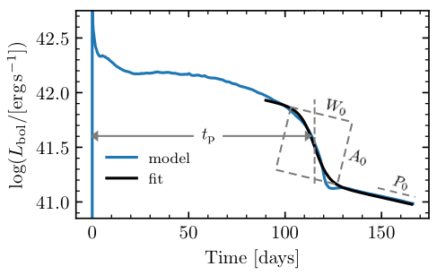
Figure 6: Diagram of fitting Equation (9) to find the 115 day duration of the plateau for our model M16.3_R608 exploded with $E_{\rm exp}=10^{51}\,{\rm ergs}$ and $M_{\rm Ni}=0.03M_{\odot}$. Fitting parameters are labelled, but we only ascribe physical significance to $t_{\rm p}$.

As the recombination-powered photosphere moves into the innermost ejecta, the optical depth at the inner boundary declines orders of magnitude and the photospheric temperature plummets. This transition, shown in Figure 7, is the physical end of the plateau. Thus, for our modeling definition of the plateau duration, we use the time, post-shock breakout, when the optical depth $\tau_{\rm IB}$ through the ejecta becomes $<10$. This time will be denoted hereafter as $t_{\tau=10}$, and can be used as a metric for plateau duration when comparing to models where there is no ${{}^{56}{\rm Ni}}$, where Equation (9) does not accurately capture the fall from the plateau. As shown by the black markers in Figure 7, the observable $t_{\rm p}$ roughly corresponds to the physical end of the plateau phase around $t_{\tau=10}$. Across all progenitor models, explosion energies, and nonzero nickel masses which we consider, RMS differences between $t_{\tau=10}$ and $t_{\rm p}$ are 4.1% and all differences are within $\pm 7\%$.

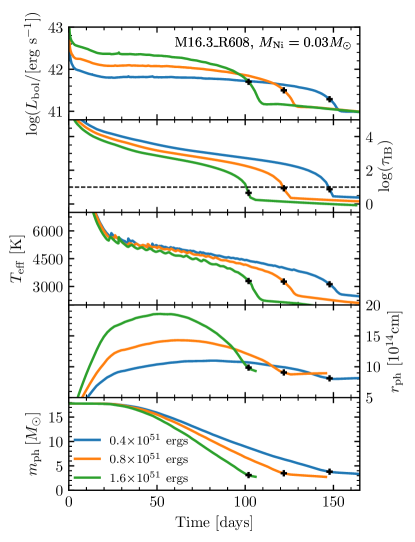
Figure 7: Evolution of luminosity, optical depth at the inner boundary ($\tau_{\rm IB}$), effective Temperature ($T_{\rm eff}$), photospheric radius ($r_{\rm ph}$), and mass coordinate of the photosphere ($m_{\rm ph}$) for our M16.3_R608 model, exploded with $M_{\rm Ni}=0.03M_{\odot}$ at three different explosion energies, showing the transition to the end of the plateau. Black plus markers indicate the end of the plateau determined from fitting Equation (9). The thin dashed line in the second panel indicates $\tau_{\rm IB}=10$.

5.1 Impact of ${{}^{56}{\rm Ni}}$ on plateau duration in our models

The presence of radioactive ${{}^{56}{\rm Ni}}$ prolongs the photospheric evolution and extends the plateau by providing extra heat to the ejecta. This is shown in Figure 8, where we show ejecta temperature profiles of the same SN explosion with different $M_{\rm Ni}$. At day 50, the photosphere for all models remains in the outer ejecta, where there is very little ${{}^{56}{\rm Ni}}$. At later times, the photosphere has moved in farther for models with lower $M_{\rm Ni}$, whereas additional heat from the ${{}^{56}{\rm Ni}}$ decay chain causes the recombination-powered photosphere to move in more slowly in models with higher $M_{\rm Ni}$.

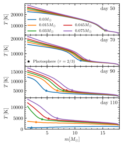
Figure 8: Ejecta temperature profiles at different times with increasing amounts of ${{}^{56}{\rm Ni}}$ for our M16.3_R608 model exploded with $10^{51}$ ergs. The location of the photosphere is shown for each model by the colored stars.

The analytics in Appendix B and Section 3 treat the ejecta as a single zone, with heating from ${{}^{56}{\rm Ni}}$ decay throughout. However, ${{}^{56}{\rm Ni}}$ is more highly concentrated in the center of the ejecta. Thus, heat from ${{}^{56}{\rm Ni}}$ decay remains trapped in the optically thick inner region, extending the plateau more at late times. This more concentrated ${{}^{56}{\rm Ni}}$ heating should have a more significant impact on the plateau duration than it would for an analytic one-zone model, as the internal energy of the inner ejecta is more relevant than that of the ejecta as a whole at the end of the plateau. Figure 9 shows the diversity of asymptotic ${{}^{56}{\rm Ni}}$ and Hydrogen distributions within our standard suite of models at handoff to STELLA for the highest-energy ($E_{\rm tot}=2\times 10^{51}\,{\rm ergs}$) highest-Nickel ($M_{\rm Ni}=0.075M_{\odot}$) cases.

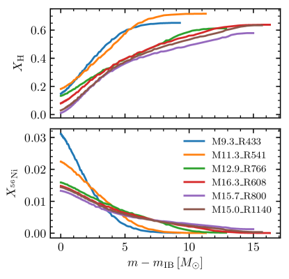
Figure 9: The diversity of H (upper panel) and ${{}^{56}{\rm Ni}}$ (lower panel) profiles for our standard suite of models, exploded with our highest $E_{\rm exp}$ and $M_{\rm Ni}$. The x-axis is the mass coordinate within the ejecta.

Moreover, the distribution of ${{}^{56}{\rm Ni}}$, which can vary amongst different progenitors depending on core structure and mixing, can also introduce inherent scatter to the plateau duration (Kozyreva et al., 2018). Figure 10 shows light curves and ${{}^{56}{\rm Ni}}$ profiles for the M16.3_R608 model exploded with $E_{\rm exp}=10^{51}\,{\rm ergs}$ and $M_{\rm Ni}=0.03M_{\odot}$, where the same ${{}^{56}{\rm Ni}}$ mass is re-distributed by hand at the time of shock breakout out to some fraction of the ejecta. Although this exercise spans a greater diversity in ${{}^{56}{\rm Ni}}$ concentration than any of our models, we see for this otherwise unexceptional light curve that the plateau duration $t_{\rm p}$ can vary by almost 10 days.

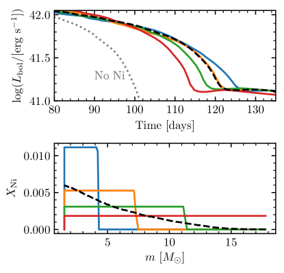
Figure 10: Light curves at the end of the plateau (upper panel) and ${{}^{56}{\rm Ni}}$ distributions (lower panel) for the M16.3_R608 model exploded with $E_{\rm exp}=10^{51}\,{\rm ergs}$ and $M_{\rm Ni}=0.03M_{\odot}$, for the fiducial explosion (black dashed line), compared to models where ${{}^{56}{\rm Ni}}$ is re-distributed by hand out to some fraction of the ejecta at the time of shock breakout (solid colored lines). The light curve for the same explosion with no Ni is given by the grey dashed line in the upper panel.

A full examination of the effects of changing the distributions in the framework of the Duffell RTI prescription (Paxton et al., 2018) is beyond the scope of this paper, and will be the subject of future study (P. Duffell et al. in Prep.). Here we examine the impact of ${{}^{56}{\rm Ni}}$ on the value of $f_{\rm rad}$ in $t_{\rm p}=t_{0}\times f_{\rm rad}^{1/6}$ (Equation (5)), where $t_{0}$ is the plateau duration for the same explosion with no ${{}^{56}{\rm Ni}}$.

Following Kasen & Woosley (2009), Sukhbold et al. (2016), and others, ${{}^{56}{\rm Ni}}$ extends the plateau as

$$t_{\rm p}/t_{0}=(1+C_{f}M_{\rm Ni}E_{51}^{-1/2}M_{10}^{-1/2}R_{500}^{-1})^{1/6},$$ (10)

we can extract $C_{f}$ by fitting to our models using the $t_{\tau=10}$ definition of plateau duration. We consider all six progenitor models with explosion energies sufficient to cause minimal fallback, with $M_{\rm Ni}/M_{\odot}$=0.0, 0.015, 0.03, 0.045, 0.06, and 0.075. We exclude models where the plateau is so long that the Nickel tail does not appear at any point in our simulations, and models which have a less than half a decade drop in $L_{\rm bol}$ from day 50 to the top of the nickel tail, as no such events have been observed.

This gives a total of 332 light curves including the 57 with no ${{}^{56}{\rm Ni}}$, which we compare to the light curves of identical explosions with no ${{}^{56}{\rm Ni}}$. Figure 11 shows the ratio of the plateau duration, $t_{\tau=10}$, of each of these light curves compared to $t_{\tau=10}$ for an identical explosion with no ${{}^{56}{\rm Ni}}$, $t_{0}$, following Kasen & Woosley (2009) but with our suite of 332 model light curves. We recover $C_{f}\approx 87$, which is an order of magnitude larger than the approximate lower bound $C_{f}\approx 7.0$ derived in Appendix B, and roughly a factor of 4 larger than $C_{f}=24$ (derived in Kasen & Woosley 2009, typographical error corrected in Sukhbold et al. 2016). This likely results from the different ${{}^{56}{\rm Ni}}$ mass distributions in our models from those in Kasen & Woosley (2009). As demonstrated in Figure 10, this can yield significant differences in the plateau duration. Our fit shows similar scatter for all ${{}^{56}{\rm Ni}}$ masses considered, with more scatter introduced by intrinsic differences among the individual models than by the changing $M_{\rm Ni}$. For $M_{\rm Ni}\gtrsim 0.03M_{\odot}$, this typically leads to a 20 - 60% increase in the plateau duration.

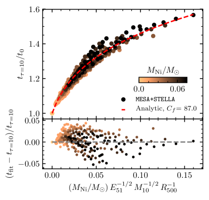
Figure 11: Plateau duration when the optical depth at the inner boundary $\tau_{\rm IB}=10$, divided by plateau duration for the same explosion with no ${{}^{56}{\rm Ni}}$, as compared to the analytic scaling Equation (10) (red dashed line) with $C_{f}$ determined from our fits. Color corresponds to $M_{\rm Ni}$ in units of solar masses. Deviations of each of the models from this relationship are shown on the lower panel.

5.2 Plateau Durations for Nickel Rich Events

For Nickel-rich events, the ${{}^{56}{\rm Ni}}$ and ${{}^{56}{\rm Co}}$ decay dominates the internal energy of the inner ejecta, such that $C_{f}M_{\rm Ni}M_{10}^{-1/2}E_{51}^{-1/2}R^{-1}>1$. Assuming that $t_{0}$ scales as in Popov (1993), we can approximate

$$\begin{split}&t_{\rm p}\propto M_{\rm ej}^{1/2}E_{\rm exp}^{-1/6}R^{1/6}\times(1+C_{f}M_{\rm Ni}M_{\rm ej}^{-1/2}E_{\rm exp}^{-1/2}R^{-1})^{1/6}\\ &\rightarrow t_{\rm p}\mathrel{\vbox{ \offinterlineskip\halign{\hfil$#$\cr\propto\cr\kern 2.0pt\cr\sim\cr\kern-2.0pt\cr}}}M_{\rm Ni}^{1/6}M_{\rm ej}^{5/12}E_{\rm exp}^{-1/4}.\end{split}$$ (11)

The two features of interest are the power law behavior and the disappearing scaling with the progenitor radius. We thus expect that the plateau duration for ${{}^{56}{\rm Ni}}$-rich events does not depend on the progenitor radius. To check, we perform a power law fit for $t_{\rm p}$ as a function of $M_{\rm Ni}$, $M_{\rm ej}$, $E_{\rm exp}$, and $R$ for 218 model light curves where $M_{\rm Ni}\gtrsim 0.03M_{\odot}$. We find that $\log(t_{\rm p}/{\rm days})=2.184+0.134\log(M_{\rm Ni})+0.429\log(M_{10})-0.280\log(E_{51})-0.018\log(R_{500})$ with RMS deviations of 2.10% and a maximum deviation of 8.1%. Since the dynamic range in $R$ is a factor of two and the scaling is negligible, we perform a fit for these same models to only $M_{\rm Ni}$, $M_{\rm ej}$, and $E_{\rm exp}$, recovering

$$\begin{split}\log(t_{\rm p}/{\rm days})=&2.184+0.134\log(M_{\rm Ni})\\ &+0.411\log(M_{10})-0.282\log(E_{51}).\end{split}$$ (12)

These coefficients are excellent matches to the power laws in Equation (11). Our models, and their agreement with this fit, are shown in Figure 12. RMS deviations between this fit and our models are 2.13%, with maximum deviation of 7.5%. Typical differences between the plateau durations recovered from the fit and those extracted from our models are $2-5$ days, with the largest discrepancy being 11 days, which is for a relatively low-luminosity SN with a plateau duration of 156 days. For all of the scaling equations of this section, the scatter in our models does not require that we report the fits to three decimal places; this is done for the sake of completeness.

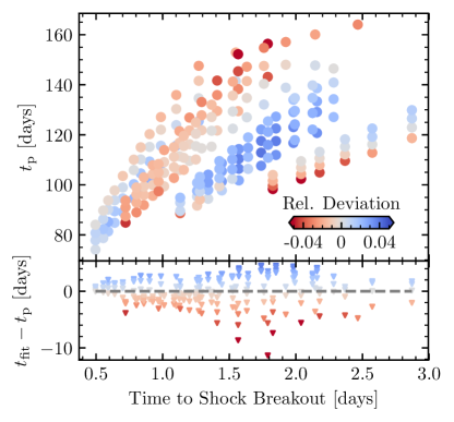
Figure 12: Plateau durations for our 218 SN light curves with $M_{\rm Ni}\gtrsim 0.03M_{\odot}$ (upper panel) and the difference in plateau duration between the model $t_{\rm p}$ and the plateau duration $t_{\rm fit}$ extracted by applying Equation (12) to the $M_{\rm ej}$, $E_{\rm exp}$, and $M_{\rm Ni}$ of each model (lower panel), colored by $(t_{\rm fit}-t_{\rm p})/t_{\rm p}$, the fractional deviation between $t_{\rm p}$ from the models and $t_{\rm fit}$. The x-axis is the time the model takes to reach shock breakout.

We also checked the agreement of Equation (12) with the publicly available light curves from Dessart et al. (2013). For all of those models where the light curve has a clear end of plateau and nickel tail, we found that our fitting formula recovers a plateau which is 7 - 20% shorter when using the values for $M_{\rm Ni}$, $M_{\rm ej}$, and $E_{\rm exp}$ reported in Dessart et al. (2013). This amounts to a difference of 8 - 27 days, with the worst agreement in the case of the low-metallicity (1/10 solar) model m15z2m3, and the best agreement in the case of their “new” s15N model. The RMS difference in $|t_{\rm p}-t_{\rm fit}|$ is 18 days, about 14% relative to the average plateau in their models.

5.3 Constraining Explosion Parameters with $ET$

Following the work of Shussman et al. (2016a), Nakar et al. (2016), Kozyreva et al. (2018), and others, we can also express the impact of ${{}^{56}{\rm Ni}}$ on $t_{\rm p}$ in terms of the ratio of the time-weighted energy contribution of the ${{}^{56}{\rm Ni}}$ decay chain to the observable quantity $ET$. This ratio is defined in Nakar et al. (2016) as

$$\eta_{\rm Ni}=\frac{\int_{0}^{t_{\rm p}}tQ_{\rm Ni}(t)\mathrm{d}t}{ET},$$ (13)

where

$$ET=\int_{0}^{\infty}t(L_{\rm bol}(t)-Q_{\rm Ni}(t))\,\mathrm{d}t,$$ (14)

is the time-weighted energy radiated away which was generated by the initial shock and not by ${{}^{56}{\rm Ni}}$ decay, and

$$Q_{\rm Ni}=\frac{M_{\rm Ni}}{M_{\odot}}\left(6.45e^{-t/8.8{\rm d}}+1.45e^{-t/113{\rm d}}\right)\times 10^{43}\ {\rm erg\ s^{-1}},$$ (15)

is the instantaneous heating rate of the ejecta due to the decay chain of radioactive ${{}^{56}{\rm Ni}}$ assuming complete trapping given in Nadyozhin (1994), and $t$ is the time in days since the explosion. It is generally assumed that $L_{\rm bol}(t)=Q_{\rm Ni}(t)$ after the photospheric phase, on the Nickel tail, and so the integral for $ET$ is often expressed to be bounded at $t_{\rm Ni}\approx t_{\rm p}$. We find this to be valid; see the lower panel of Figure 13.

Figure 13 shows the impact of ${{}^{56}{\rm Ni}}$ on light curves and the integrated $ET$ for the M16.3_R608 model exploded with $E_{\rm exp}=10^{51}\,{\rm ergs}$ at different $M_{\rm Ni}$. The lower panel gives the cumulative $ET$, integrated from shock breakout to the time on the x-axis. Most of the contribution to $ET$ comes from luminosity on the plateau, with little contribution at early times ($t<20\,{\rm d}$) and no contribution from the Nickel tail. In the very ${{}^{56}{\rm Ni}}$-rich case, the cumulative integral may dip slightly negative around day 20, as radiative cooling is briefly less efficient than heating from the ${{}^{56}{\rm Ni}}$ decay chain ($L_{\rm bol}<Q_{\rm Ni}$ in this region). This is more pronounced in models exploded at lower energies. As expected, although heating from the radioactive decay chain of ${{}^{56}{\rm Ni}}$ extends the plateau and elevates the Nickel tail, it has very little impact on the final integrated value of $ET$ calculated from our model light curves. Indeed, the variations of $ET$ for the same explosion but different ${{}^{56}{\rm Ni}}$ are at a few per-cent level.

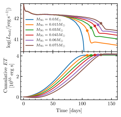
Figure 13: Impact of ${{}^{56}{\rm Ni}}$ on $L_{\rm bol}$ (upper panel) and cumulative $ET$ integrated from shock breakout to the time on the x-axis (lower panel) for M16.3_R608 model exploded with $E_{\rm exp}=10^{51}\,{\rm ergs}$ and $M_{\rm Ni}/M_{\odot}=0.0,\ 0.015,\ 0.03,\ 0.045,\ 0.06,$ and 0.075. Points indicate $t_{\rm p}$ for the events where $M_{\rm Ni}>0.0M_{\odot}$.

Dimensionally, using the Popov scalings for $L_{50}$ and plateau duration with no ${{}^{56}{\rm Ni}}$ ($t_{0}$), $ET$ is expected to scale as

$$ET\propto L_{50}t_{0}^{2}\propto M_{\rm ej}^{1/2}E_{\rm exp}^{1/2}R,$$ (16)

and thus $\eta_{\rm Ni}$ should scale as $M_{\rm Ni}/ET$. A more detailed derivation of this same scaling is given in Shussman et al. (2016a). This recovers the extension to the plateau duration given by Equation (10), recast as

$$t_{\tau=10}/t_{0}=(1+a\eta_{\rm Ni})^{1/6},$$ (17)

where the scaling factor $a$ can be fit from models and encodes information about the internal structure of the ejecta, and in particular the concentration of ${{}^{56}{\rm Ni}}$. Kozyreva et al. (2018) find that for typical models, $a\approx 4$ (their Figure 5). Figure 14 shows the extension of the plateau as a function of $\eta_{\rm Ni}$ in our models. We find slightly higher values for $a$, with more models falling along $a\approx 5.5$, indicating a larger impact of ${{}^{56}{\rm Ni}}$ on the plateau duration, in part because $\eta_{\rm Ni}$ encodes information about ${{}^{56}{\rm Ni}}$ mixing, and our models make use of the Duffell RTI prescription whereas mixing is parameterized in Kozyreva et al. (2018). We show good agreement with the functional form in Equation (17).

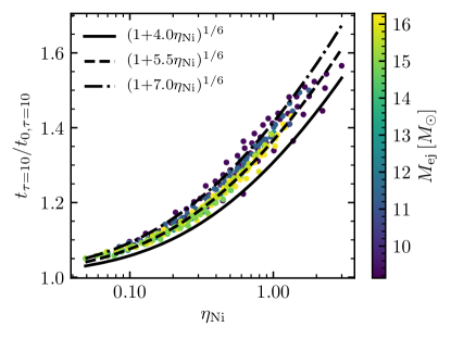
Figure 14: Plateau duration for models with ${{}^{56}{\rm Ni}}$ relative to the same explosion with no ${{}^{56}{\rm Ni}}$, versus the parameter $\eta_{\rm Ni}$. Color corresponds to ejecta mass, and can be used to distinguish between the individual progenitor models. Black lines correspond to the plateau extension factor $(1+a\eta_{\rm Ni})^{1/6}$ for different values of $a$.

For SNe with a reasonably well-sampled bolometric light curve where $M_{\rm Ni}$ is measured from the Nickel tail, $ET$ can be calculated and used to constrain $M_{\rm ej}$, $E_{\rm exp}$, and progenitor $R$ for a given explosion. In addition, $ET$ can provide a critical constraint for explosions with lower $M_{\rm Ni}$, where the ${{}^{56}{\rm Ni}}$ decay chain does not dominate the internal energy of ejecta and thus the simple power law of Equation (12) should not apply. Although observationally $M_{\rm Ni}$ must be extracted from the Nickel tail in order to calculate $ET$, $ET$ does not follow any scaling with $M_{\rm Ni}$, as it subtracts the contribution of ${{}^{56}{\rm Ni}}$ heating in the light curve evolution.

To determine how $ET$ scales with $M_{\rm ej}$, $E_{\rm exp}$, and $R$ in our models, we use the same 218 model light curves as with $t_{\rm p}$ in Equation (12), to recover

$$\begin{split}\log(ET/{\rm erg\,s})=&55.460+0.299\log(M_{10})\\ &+0.435\log(E_{51})+0.911\log(R_{500})\end{split}$$ (18)

for our suite of models, which does not include interactions CSM. This scaling has a slightly shallower dependence on $M_{\rm ej}$, $E_{\rm exp}$, and progenitor $R$ than Equation (16). The agreement between our models and Equation (18) is shown in Figure 15. RMS deviations between our models are 5.0%, with a maximum deviation of 12.4%. Although the fit was performed on models with $M_{\rm Ni}\gtrsim 0.03M_{\odot}$ to be consistent with our set of models for $t_{\rm p}$, the recovered scaling applies similarly well for our models with $M_{\rm Ni}<0.03M_{\odot}$, with RMS deviations of 5.3% and all deviations under 20%. The overlapping black rings in Figure 15 show the typical scatter in values of $ET$ for the same explosion when varying $M_{\rm Ni}$. Each set of overlapping rings corresponds to $ET$ for a single progenitor model exploded with a single $E_{\rm exp}$, but with different values of $M_{\rm Ni}$. This scatter in $ET$ when only varying $M_{\rm Ni}$ is well within the scatter between the models and the fitted Equation (18).

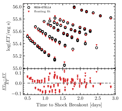
Figure 15: Calculated values of $ET$ for 218 SN light curves and the values recovered with the fitted Equation (18) (upper panel), and fractional deviations between $ET$ in the models and recovered using Equation (18) (lower panel).

6 Observed Velocity Evolution

We now discuss the diagnostic value of the material velocity inferred from the absorption minimum of the Fe II 5169Å line, often measured and reported at day 50, $v_{\rm Fe,50}$. Ideally, the measured Fe line velocities would provide an additional quantitative measurement that would allow for estimation of progenitor and explosion properties (Pejcha & Prieto, 2015a; Müller et al., 2017). However, as we show here, these measurements are highly correlated with bolometric luminosity measurements at a fixed time on the plateau, and are largely redundant at day 50. If there is no substantial CSM around the star, than earlier time ($\lesssim 20$ day) measurements may prove more useful (see Section 7.2).

The Fe II 5169Å velocity is typically used to approximate the velocity at the photosphere ($v_{\rm Ph}$), although there is substantial evidence that measured line velocities are typically higher than that predicted for the model photosphere ($\tau=2/3$) (e.g. Utrobin et al. 2017; MESA IV). In a homologously expanding medium, the strength of a given line is quantified using the Sobolev optical depth (Sobolev, 1960; Castor, 1970; Mihalas, 1978; Kasen et al., 2006), which accounts for the shift in the line profile due to the steep velocity gradient in the ejecta. This is captured in MESA+STELLA following MESA IV, where the $\tau_{\rm Sob}=1$ condition is used to measure iron line velocities ($v_{\rm Fe}$). Although in the following we discuss both this velocity and the velocity at the model photosphere, we recommend using $v_{\rm Fe}$ defined when $\tau_{\rm Sob}=1$ when comparing to observations.

6.1 Velocities in Explosion Models

When the velocity profile of the ejecta becomes fixed in time, this material is said to be in homologous expansion. Analytically, homology is often approximated $r=vt$ for a fluid element at radial coordinate $r$ with velocity $v$ at time $t$. While not quite true for material in the center of the ejecta, which is expanding more slowly and therefore the initial radial coordinate is still relevant, this approximation generally holds for faster-moving material which has experienced more significant expansion at a given time, as well as for the slower-moving material at late times when it is becoming visible. This is reflected in Figure 32 of MESA IV.

Many software instruments devoted to modeling radiative transfer, such as Sedona, assume homologous expansion in the true sense of a fixed velocity profile. Figure 16 shows the extent to which this is satisfied in our M16.3_R608 model exploded with $10^{51}\,{\rm ergs}$. The upper panel shows the relative error in predicting the radial coordinate of a fluid element at day 160 by assuming $r_{\rm h}({\rm day\ 160})~{}=~{}r(t_{0})~{}+~{}v(t_{0})(160{\rm d}-t_{0})$ for homology starting at $t_{0}$ = days 10, 20, and 50. We define $\Delta r_{160}=r_{160}-r_{\rm h}(\rm day160)$, where $r_{160}=$ the true radius of that fluid element at day 160 in STELLA. The lower panel shows the deviation between the velocity profiles at days 10, 20, and 50, and that at day 160. Before homology, the innermost material is moving slightly faster than its day 160 value, and the outer material is moving slightly slower. Even in the envelope, there is deviation between the day 10 velocity profile and day 160 at the level of a few per-cent. By day 20 this falls below 2%, and by day 50 typical deviations of the velocity profile in the bulk of the ejecta from the velocity profile at day 160 are at the level of 0.5%. Generally, by day 20, the difference in predicted radial coordinate of the half-mass fluid element at day 160 is below 3% of its true value in the hydrodynamical simulation. At this time the radial coordinate predicted for day 50 is also within 2% of its true value at day 50.

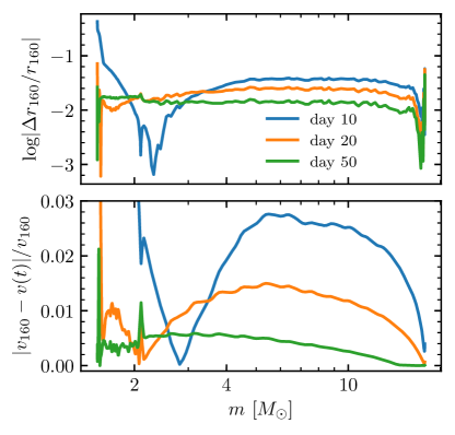
Figure 16: Agreement between hydrodynamical models and homologous expansion. The upper panel shows the relative error in predicting the radial profile day 160 by assuming homology starting at days 10, 20, and 50, compared to the true radial coordinate at day 160 in STELLA. The lower panel shows the absolute relative deviation between the velocity profiles at days 10, 20, and 50, and the profile at day 160.

Figure 17 shows approximately homologous velocity profiles (taken here at day 50) scaled by the square root of $E_{\rm exp}$ for all 6 progenitor models at all energies that cause sufficiently little fallback. Each family of colored lines reflects explosions of an individual model, and each of the 6 families of lines contains the profiles for multiple explosion energies for that model. When looking at any fixed mass coordinate within a single progenitor model, the fluid velocity divided by $\sqrt{E_{\rm exp}}$ is constant. Moreover, as shown in Figure 18, looking at the same dimensionless mass coordinate inside the ejecta and scaling also by the square root of $M_{\rm ej}$, this relationship holds for any dimensionless ejecta mass coordinate throughout the entire velocity profile, with small variations only near the inner boundary, where the reverse shock becomes relevant and where fallback has a greater effect.

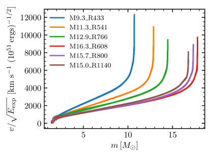
Figure 17: Day 50 velocity profiles in STELLA, divided by the square root of $E_{\rm exp}$, versus mass coordinate for 6 unique progenitor models with a variety of explosion energies. Each colored line represents a different model, and lies on top of a collection of $6-12$ nearly identical lines which correspond to different explosion energies for the same progenitor model.

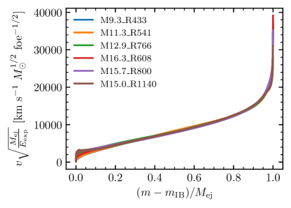
Figure 18: Day 50 velocity profiles in STELLA, multiplied by $\sqrt{M_{\rm ej}/E_{\rm exp}}$, versus dimensionless ejecta mass coordinate for all 57 explosions with energies sufficient to yield little fallback. For a fixed fractional position within the ejecta, velocities obey the scaling in Equation (19).

Popov (1993), Pejcha & Prieto (2015a), and others, have often assumed that

$$E_{\rm exp}\approx\frac{1}{2}M_{\rm ej}v_{\rm Ph,50}^{2},$$ (19)

where $v_{\rm Ph,50}$ is the photospheric velocity at day 50, in order to close the system of equations for $L_{50}$ and $t_{\rm p}$ as a function of $M_{\rm ej}$, $E_{\rm exp}$ and progenitor radius $R$. While the scaling law suggested in Equation (19) holds for the fluid velocity at a fixed dimensionless ejecta mass coordinate, as shown in Figure 18, as the photosphere moves deeper into the ejecta, it does not probe velocities at the same mass coordinate at a given time post shock-breakout. Rather, at a fixed time in the evolution, faster-expanding ejecta in higher energy explosions allows the observer to see deeper mass coordinates, compared to a lower energy explosion of the same star. This is evident in Figure 19, which shows velocity profiles for the M16.3_R608 model at 5 different explosion energies, marking the location of the photosphere and Fe II 5169Å line at fixed times. As a result of the expanding ejecta, we expect a shallower scaling for velocity as a function of energy at fixed mass than the naive $v_{\rm Ph,50}\propto E_{\rm exp}^{1/2}$. Indeed a linear fit for a single model with fixed ejecta mass and radius finds shallower scalings: $v_{\rm Ph,50}\propto E_{\rm exp}^{0.36}$, and $v_{\rm Fe,50}\propto E_{\rm exp}^{0.30}$. These scalings approximately hold for the other individual models.

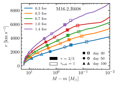
Figure 19: Day 50 velocity profiles versus overhead mass coordinate in STELLA for our M16.3_R608 model at 5 different explosion energies. We have included photospheric (filled markers) and Fe II 5169Å line velocities (open markers) for day 30, 50, and 100 as denoted by shape of the marker.

Additionally, a simple velocity scaling with $M_{\rm ej}$ and $E_{\rm exp}$ becomes murkier when comparing across models of different masses at fixed explosion energy, since there is no reason for the same explosion energy to yield the “same” mass coordinate at the same time in two different progenitors. In fact, as seen in Figure 20, $v_{\rm Fe}$ and $v_{\rm Ph}$ at day 50 are not even monotonic in $M_{\rm ej}$ for different stars at fixed $E_{\rm exp}$. Thus, we cannot derive any power law for $v_{\rm Ph,50}$ or $v_{\rm Fe,50}$ solely as a function of $M_{\rm ej}$ and $E_{\rm exp}$. As we show in the following section, additional dependences are relevant (Equation 20).

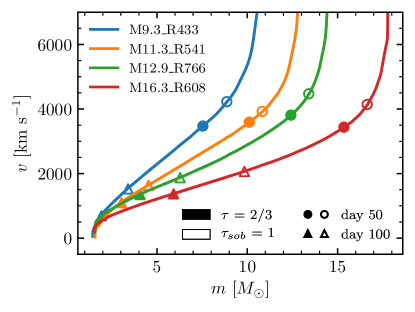
Figure 20: Day 50 velocity profiles for 4 different models all exploded with an energy of $1.0\times 10^{51}$ ergs. Filled markers indicate the location of the photosphere and open markers indicate where the Fe II 5169Å line is formed. Velocities at days 50 and 100 are denoted by the shape of the marker.

6.2 $L_{50}$ - $v_{\rm Ph,50}$ Relation

This result highlights a true degeneracy, discovered observationally by Hamuy (2003) and explained by Kasen & Woosley (2009). We start with the Stefan-Boltzmann formula for luminosity, $L=4\pi R_{\rm phot}^{2}\sigma T_{\rm eff}^{4}$, where $R_{\rm phot}$ is the photospheric radius, and note that $T_{\rm eff}$ is roughly constant at the photosphere and set by H recombination to $T_{\rm eff}\approx$ 6000 K. At fixed time on the plateau, (e.g. day 50) while the ejecta is expanding homologously with radial position $r\approx vt$ for any given mass coordinate, for the photosphere at day 50 $L_{50}\propto v_{\rm Ph,50}^{2}$ and so $v_{\rm Ph,50}\propto\sqrt{L_{50}}$. In this way, the luminosity, together with homologous expansion, sets the location of the photosphere within the expanding ejecta, which in turn sets the velocity measured at or near the photosphere.

Figure 21 shows $v_{\rm Ph,50}$ and $v_{\rm Fe,50}$ versus $L_{50}$ for all 57 explosions which experience sufficiently little fallback (6 models with 6-12 explosion energies each). Also plotted are data from Pejcha & Prieto (2015b) and Gutiérrez et al. (2017). In both observational data sets, velocities are inferred from the Fe II 5169Å line, suggesting that these velocities are better captured in our models at $\tau_{\rm Sob}\approx 1$, rather than assuming the line is formed at the photosphere ($\tau=2/3$). We also see good agreement between our models and the scaling $v_{\rm Ph,50}\propto\sqrt{L_{50}}$.

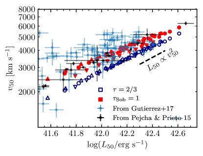
Figure 21: Velocity versus Luminosity at day 50 for a variety of progenitor models and explosion energies. Open navy blue markers denote photospheric velocities ($\tau=2/3$) and closed red markers denote Fe II 5169 Å velocities ($\tau_{\rm Sob}=1$). Points with error bars are data from 2 samples: Gutiérrez et al. (2017) (blue) and Pejcha & Prieto (2015b) (black).

It is therefore unsurprising that the Fe velocities during the plateau phase match the data for a model with a luminosity match at day 50. This was seen in Section 6 of MESA IV, Figure 42, where two models with light curve agreement with SN199em show identical velocity evolution. Figure 22 shows the luminosity and velocity of those two progenitor models, renamed M12.9_R766 and M16.3_R608 in our suite, blown up with slightly adjusted explosion energies to produce even better light curve agreement. In the case where models match closely in both $L$ and $t_{p}$, the agreement in velocity is excellent throughout the evolution of the SN.

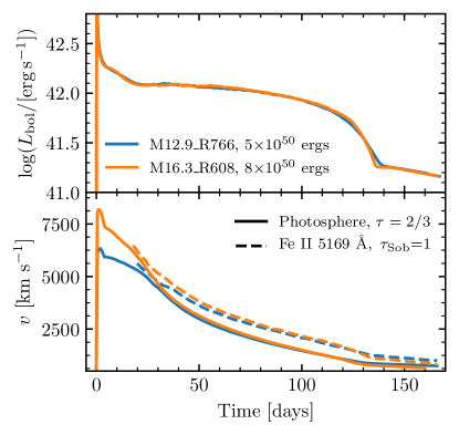
Figure 22: Luminosity and velocity for the 99em_16 (renamed M12.9_R766) and 99em_19 (renamed M16.3_R608) models from Paxton et al. (2018) with different explosion energies in order to attain light curve agreement.

As with $L_{50}$ in Section 4, we fit a power law for $v_{50}$ as a function of $M_{\rm ej}$, $E_{\rm exp}$, and $R$ to our models with constant nickel mass $M_{\rm Ni}=0.03M_{\odot}$. We do this with both $v_{\rm Fe,50}$ and $v_{\rm Ph,50}$ at day 50, noting that observationally, $v_{\rm Fe,50}$ is the relevant scaling. For the photospheric velocity at day 50, we found power laws that are very similar to the scaling found if $v_{\rm Ph,50}\propto L_{50}^{1/2}$:

$$\begin{split}&\log(v_{\rm Ph}/{\rm km\ s^{-1}})=\\ &3.54-0.19\log M_{10}+0.36\log E_{51}+0.32\log R_{500},\end{split}$$ (20)

where the prefactor and power law coefficients are all fit from our models.

This is valuable insofar as it reinforces the degeneracy highlighted in Figures 21 and 22, but, as discussed, this velocity is unmeasurable, and observed Fe II 5169Å line velocities are better estimated by ($\tau_{\rm Sob}=1$). A similar fit to $v_{\rm Fe}$ at day 50,

$$\begin{split}&\log(v_{\rm Fe,50}/{\rm km\ s^{-1}})=\\ &3.61-0.12\log M_{10}+0.30\log E_{51}+0.25\log R_{500},\end{split}$$ (21)

yields higher predicted velocities everywhere, and shows somewhat shallower dependence on each of the explosion properties. The model Fe line velocities and their residuals as compared with Equation (21) are shown in Figure 23.

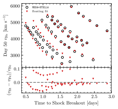
Figure 23: Model $v_{{\rm Fe}}$ ($\tau_{\rm Sob}=1$) at day 50, and velocities recovered with the fitting formulas (upper panel), and their residuals (lower panel) for our suite of 57 explosions with $M_{\rm Ni}=0.03M_{\odot}$. So as to clarify the model space, we use time to shock breakout as the x-axis.

Although the degeneracy is less pronounced for $\tau_{\rm Sob}=1$ than for the photosphere, with some scatter in Figure 21 and differences in the recovered power laws, this scatter is small compared to intrinsic variations in luminosity and plateau duration, and is therefore insufficient to break the degeneracy between $v$ and $L$ in order to provide accurate estimates for $M_{\rm ej}$, $E_{\rm exp}$, and $R$. It is for this reason that we do not advocate using measured velocities at day 50 to infer explosion properties.

7 Families of Explosions

7.1 Inverting Our Scalings

Due to the degeneracies highlighted in Section 6, we cannot simply extract $M_{\rm ej}$, $E_{\rm exp}$, and $R$ from light curve measurements and $v_{\rm Fe,50}$. Attempting to invert all three scalings (Equations (8), (18), and (12)) is ill-conditioned and within the scatter within our models. However, we can use the scalings to solve for two of the three relevant explosion properties as a function of the third, revealing a family of possible explosions that yield nearly identical bolometric light curves.

SNe with direct progenitor observations are improving with time, so we solve Equations (8) and (12) for $M_{\rm ej}$ and $E_{\rm exp}$ as a function of $M_{\rm Ni}$, $L_{50}$, $t_{\rm p}$, and $R$, to find

$$\begin{split}\begin{aligned} \log(E_{51})&=-0.728+2.148\log(L_{42})-0.280\log(M_{\rm Ni})\\ &+2.091\log(t_{\rm p,2})-1.632\log(R_{500}),\\ \log(M_{10})&=-0.947+1.474\log(L_{42})-0.518\log(M_{\rm Ni})\\ &+3.867\log(t_{\rm p,2})-1.120\log(R_{500}),\end{aligned}\end{split}$$ (22)

where $M_{\rm Ni}$ is in units of $M_{\odot}$, $L_{42}=L_{50}/10^{42}$ erg s^-1 and $t_{\rm p,2}=t_{\rm p}/100\,{\rm d}$. Alternatively, we can use a measured $ET$ rather than $t_{\rm p}$ to find

$$\begin{split}\begin{aligned} \log(E_{51})&=-0.587-1.497\log(R_{500})\\ &+1.012\log(ET_{55})+0.756\log(L_{42}),\\ \log(M_{10})&=-0.685-0.869\log(R_{500})\\ &+1.872\log(ET_{55})-1.101\log(L_{42}),\end{aligned}\end{split}$$ (23)

where $ET_{55}=ET/10^{55}{\rm erg\,s}$.

Before demonstrating how to apply these fitting formula to observed SNe, we show how well modeled events can be matched. The upper panel of Figure 24 shows the fraction of models with light curve properties matching their fitted values (applying Equations (8), (12), and (18)) within a given deviation tolerance shown on the x-axis. The lower panel shows the fraction of models in which we can recover the values of $M_{\rm ej}$ and $E_{\rm exp}$ within a given deviation tolerance by applying Equation (22) (solid lines) or Equation (23) (dashed lines) to the model light curve observables and $R$. Given that there is no statistical meaning to the sample of models beyond probing different regions of parameter space, this merely provides a heuristic guide to how well our sample of models match with the fitted formulae.

Applying Equation (22) using $t_{\rm p}$ to our suite of Nickel-rich SNe, we recover $M_{\rm ej}$ and $E_{\rm exp}$ with RMS deviations between the models and the fits of 10.7% and 10.4%, respectively, with maximum deviations of 35% and 27%. Using $ET$ and Equation (23), we recover $M_{\rm ej}$ and $E_{\rm exp}$ with RMS deviations between the models and the fits of 7.3% and 7.6%, respectively, with maximum deviations of 16% and 18%. Although the modeling uncertainties for the inverted $ET$ scalings are smaller than those which use $t_{\rm p}$, the observable uncertainty is greater and may be accompanied by an offset, as excess emission within the first 10-40 days due to interaction with CSM may cause an excess in $ET$ as compared to our models.

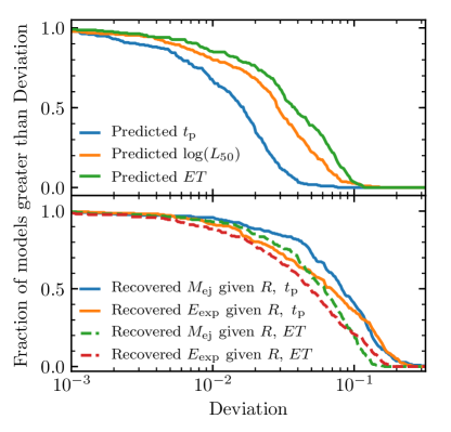
Figure 24: Distribution of deviations between our models and Equations (8) and (12) (upper panel), and the distribution of deviations between recovered values of $M_{\rm ej}$ and $E_{\rm exp}$ by applying the inverted scalings (Equation (22)) to the model light curve properties and radii, and the models themselves (lower panel). This gives a heuristic for the agreement between the fitted formulae and our suite of models.

Using these relations, we now show how very comparable light curves (and thus comparable Fe II 5169Å line velocities on the plateau) can be produced with different progenitors exploded at different energies. Figure 25 shows an example of the family of models in $M_{\rm ej}-E_{\rm exp}$ parameter space as a function of $R$ that could produce an “observed” SN light curve with $\log(L_{50}/{\rm erg\,s^{-1}})$=42.13, $\log(ET/{\rm erg\,s})$=55.58, $t_{\rm p}$=123, and $M_{\rm Ni}=0.045M_{\odot}$, which are the values matching a randomly selected model out of our suite: the M12.9_R766 model exploded with $E_{\rm exp}=6\times 10^{50}$ ergs and that $M_{\rm Ni}$.

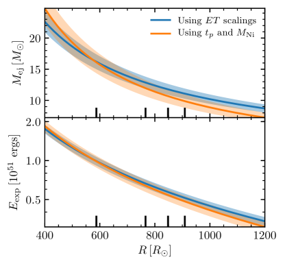
Figure 25: Degeneracy curves applying Equation (22) (orange) and Equation (23) (blue) as a function of progenitor radius $R$ for an “observed” SN with $\log(L_{50}/{\rm erg\,s^{-1}})$=42.13, $\log(ET/{\rm erg\,s})$=55.58, $t_{\rm p}$=123, and $M_{\rm Ni}=0.045M_{\odot}$. The shaded region corresponds to the RMS deviations between our models and the values recovered by applying Equations (22) and (23). Short black lines correspond to the radii of the M17.8_R587, M12.9_R766, M10.2_R848, and M9.8_R909 models, which produce the light curves, velocities, and $ET$ evolution shown in Figure 26.

To exhibit how this exercise would proceed, we constructed three additional models consistent with the bands in Figure 25, based off Equation (22) using $t_{\rm p}$. We then explode these progenitor models with $E_{\rm exp}$ as dictated by the degeneracy curve. We created multiple such models: one with $M_{\rm ej}=17.8M_{\odot}$ and $R=587R_{\odot}$, which we explode with $1\times 10^{51}$ ergs, one with $M_{\rm ej}=10.2M_{\odot}$ and $R=848R_{\odot}$, which we explode with $5\times 10^{50}$ ergs, and one with $M_{\rm ej}=9.8M_{\odot}$ and $R=909R_{\odot}$, which we explode with $4.5\times 10^{50}$ ergs. The values of $R$ for these three models, and for M12.9_R766 exploded with $6\times 10^{50}$ ergs, are shown as black tick marks in Figure 25. Figure 26 shows the resulting light curves, velocities, and accumulated ETs. We see very good agreement in $L_{50}$ and along the plateau, and recover $t_{\rm p}$ values from 120 to 125 days for all four light curves.

The values of $ET$ for three of the four light curves agree within $\approx 2$%, ranging from 3.75 to 3.84$\times 10^{55}$ erg s; however, the $5\times 10^{50}$ erg explosion of the M10.2_R848 model has a value of $ET$ which is noticeably higher, at 4.26$\times 10^{55}$ erg s. Additionally, velocities agree on the plateau, and thus cannot be used to break the light curve degeneracy, which at least spans a factor of 2 in explosion energy, nearly a factor of 2 in $M_{\rm ej}$, and a factor of 1.5 in progenitor $R$. This captures much of the parameter space in which IIP SNe from RSG progenitors could be produced to begin with!

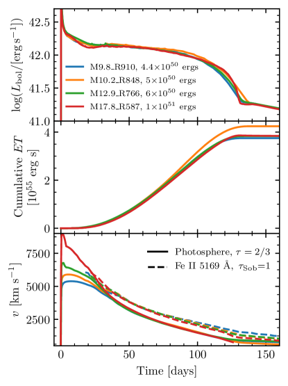
Figure 26: Light curves, cumulative ET, and velocities for four different explosions which yield nearly the same $L_{50}$, $t_{\rm p}$, and velocities at day 50.

7.2 The Importance of Velocities at Early Times

Although velocity measurements at day 50 are largely degenerate with measurements of $L_{50}$, as discussed in detail in Section 6, early time velocities up to day $\approx$20 could be used to distinguish between low-energy explosions of large-radius lower-mass RSGs and high-energy explosions of compact-radius high-mass RSGs in cases where there is minimal CSM present. As seen in the lower panel of Figure 26, higher energy explosions of compact stars yield faster velocities at early times. Before around day 20, the radial coordinate of the photosphere is moving outward, and the declining photospheric temperature is set by shock cooling rather than by recombination. Thus in this phase the velocity measured near the photosphere is not dictated by the plateau luminosity as it is at day 50. Early light curves and photospheric velocities are discussed in detail by Morozova et al. (2016) and Shussman et al. (2016b). Shussman et al. (2016b) find an expression for the photospheric velocity at early times as a function of $M_{\rm ej}$, $E_{\rm exp}$, and $R$ (their Equation 48), assuming that the density profile of the progenitor model behaves like a power law in radial coordinates. After the photosphere leaves the so-called breakout shell ($5{\rm d}\lesssim t\lesssim 20{\rm d}$), Shussman et al. (2016b) find that $v_{\rm Ph}(t)/{\rm km\,s^{-1}}\approx 1.2\times 10^{4}M_{15}^{-0.3}E_{51}^{0.38}R_{500}^{-0.14}t_{\rm d}^{-0.2}$ where $M_{15}=M_{\rm ej}/15M_{\odot}$ and $t_{\rm d}=t/{\rm d}$. At day 15 this equation describes our full suite of models with RMS deviations of 5.5% and with all deviations under 15%.

As is also seen in Figure 2 of Morozova et al. (2016), no single power law fully describes progenitor density profiles around the photospheric mass coordinate in our models for any fixed time in the light curve evolution. Nonetheless our entire suite of models, which does not include the presence of circumstellar material, can approximately be described by the fitted power law

$$\begin{split}\log(v_{\rm Ph,15})=&3.90-0.22\log(M_{10})\\ &+0.43\log(E_{51})-0.13\log(R_{500}),\end{split}$$ (24)

where $v_{\rm Ph,15}$ is the photospheric velocity at day 15 in km s^-1, with RMS deviations of 3.7% and a maximum deviation of 10% between the models and Equation (24). The dynamic range in $v_{\rm Ph,15}$ in our models is a factor of $\approx 3$, ranging from $\approx 4,000-12,000$ km s^-1.

Although Equation (24) and Shussman’s Equation 48 describe our models well, we warn the reader that velocities at this time are sensitive to the density structure of the outermost ejecta including any asphericity, as well as any interactions with any circumstellar material present. Thus more work is needed in order to faithfully capture the early-time velocities and their dependence on the relevant properties of the explosion, especially in cases where CSM is present. Nonetheless, early time velocity measurements could in principle provide a third constraint and break the light curve degeneracies, thus allowing an inference of $M_{\rm ej}$, progenitor $R$, and $E_{\rm exp}$ for a given observed Type IIP SN.

8 Concluding Remarks

We have shown the utility of using MESA+STELLA to model an ensemble of Type IIP SN progenitors, a capability introduced by Paxton et al. (2018). We introduced new best-fit scaling laws for the plateau luminosity at day 50, $L_{50}$ (Equation 8), and for the duration of the plateau $t_{\rm p}$ in the limit of Nickel-rich ($M_{\rm Ni}\geq 0.03M_{\odot}$) events (Equation 12) as a function of ejecta mass, explosion energy, and progenitor radius. We also recovered a similar fit for the observable $ET$ (Equation 18). Velocity measurements on the plateau cannot be simply described by $v_{\rm Ph,50}\approx(2E_{\rm exp}/M_{\rm ej})^{1/2}$ assumed by Popov (1993) or the scaling given in Litvinova & Nadyozhin (1983), but rather scale with $L_{50}$ as noted by Hamuy (2003); Kasen & Woosley (2009) and others, shown in our Figure 21. While early-time velocities observed during the photospheric phase ($\approx$ day 15) could provide a promising third independent constraint on $M_{\rm ej}$, $E_{\rm exp}$, and $R$, these velocities can be affected by interaction with CSM, deviations from spherical symmetry, and the specifics of the density profile of the progenitor star. Thus early velocities require more work in order to simply interpret in observed systems. Presently, given a bolometric light curve, one can at best recover a family of explosions which produce comparable light curves and thereby velocities on the plateau, as demonstrated in Figures 22 and 26. This can then be used to guide modeling efforts, especially when coupled with other constraints, such as a measurement of the core mass and thereby progenitor mass at the time of explosion (as in Jerkstrand et al. 2012). With a clear independent constraint on one explosion parameter, such as an observed progenitor radius, the other explosion properties can be simply recovered to around 15%.

Appendix A Quantifying Fallback in Core-Collapse Supernovae

Here we discuss modifications relative to MESA IV, of MESA modeling of the ejecta evolution after core collapse in massive stars (roughly M $>8M_{\odot}$). These are focused on cases where the total final explosion energy is positive, but insufficient to unbind the entirety of the material which does not initially collapse into the compact object. In these weak explosions, there is some amount of fallback material which does not become unbound. Our emphasis here is to quantify and remove fallback in model explosions of RSG progenitor stars. Although we describe models of Type IIP SN explosions, this scheme can be similarly applied to core collapse events in massive stars which have lost the majority of their outer Hydrogen envelope, which produce Type IIb and Ib SNe.

In MESA IV, three options existed to treat fallback:

1. Set the velocity of all inward-moving material with negative total energy to be zero, which creates a hydrostatic shell that can be excised from the ejecta before handing off to the radiation hydrodynamics code STELLA to calculate SN observables.

2. During the shock propagation phase, remove material at the inner boundary (IB) if it has negative velocity (i.e. if it is infalling).

3. Remove material at the IB if it is moving with negative velocity and also has net negative energy (i.e. it is bound and infalling).

However, triggering fallback based only on conditions in the innermost zone can lead to problems. For example, in many models at lower explosion energies, while the innermost zone may have negative cell-centered velocity, it can be in thermal contact with neighboring zones. Therefore to remove cells solely based upon their having negative velocity creates a vacuum at the IB which can remove energy and mass which could otherwise remain in the ejecta. Moreover, energy deposited at the IB by any inward-propagating shock can cause the innermost zones to have positive total energy, while being surrounded by a larger amount of material with net negative energy. Because of this, in some models, checking only if the innermost zone is bound before triggering fallback can lead to bound material piling up on top of a small number of cells with positive total energy. If not removed this can lead to a globally bound hydrostatic shell building up in the center, which might interact with the ejecta and affect concentrations of important species such as H and ${{}^{56}{\rm Ni}}$, thus affecting SN properties. Such a region can also lead to numerical problems if not properly excised before handing off to radiative transfer codes such as STELLA.

Paxton et al. (2019) (MESA 5) introduces two new user controls to better account for material which could fall onto the central object during the hydrodynamical evolution of low explosion energy core-collapse SNe. First, a new criterion is implemented to select which material is excised from the model. At each timestep, MESA calculates the integrated total energy from the innermost cell to cell $j$ above it:

$$E_{j}=\sum_{i={\rm inner}}^{j}\left[e_{i}-\frac{Gm_{i}}{r_{i}}+\frac{1}{2}u_{i}^{2}\right]{\rm d}m_{i},$$ (A1)

where for cell $i$ at mass $m_{i}$ and radius $r_{i}$, $e_{i}$ is the internal energy in erg g^-1 and $u_{i}$ is the velocity in cm s^-1. If $E_{j}<0$, then there is a bound inner region, and MESA continues this calculation outward until it reaches a cell $k$ with local positive total energy ($e_{k}-Gm_{k}/r_{k}+u_{k}^{2}/2>0$), causing the integral to be at a local minimum. MESA deletes material inside this zone, and moves the IB, fixing the inner radius of zone $k$ to be the new radius of the inner boundary r_center, and setting the velocity at the inner boundary v_center=0. A schematic diagram of this calculation, in a case where fallback is triggered but the innermost zones are unbound, is shown in Figure 27.

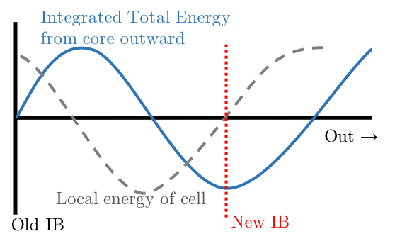
Figure 27: Diagram for new fallback criterion at a timestep where there is net positive energy near the inner boundary, but a larger, gravitationally bound region above it which will eventually fall back.

Figure 28 shows the evolution of the inner boundary for explosions of varying total energy just after the explosion ($E_{\rm tot}$, defined in Section 2), using the new fallback criterion for the M12.9_R766 progenitor model, which has a total energy of $-4.4\times 10^{50}$ ergs just before the explosion. Nearly all of the mass lost to fallback occurs while the forward-moving shock is in the Helium layer, beginning around the time that the reverse shock generated at the interface between the CO/He layers reaches the inner boundary. Because the new fallback prescription sets v_center=0 and fixes r_center except in the case of fallback being triggered, all changes in the radius of the inner boundary are due to cells being removed from the inner boundary. For sufficiently large explosion energies, little to no fallback is seen, although some cells of negligible mass are removed from the inner boundary, causing the radius of the inner boundary to move outward.

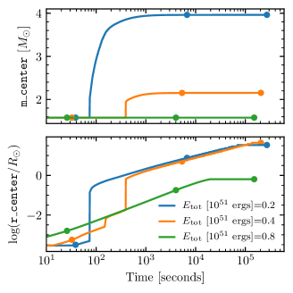
Figure 28: Evolution of the mass (upper panel) and radial (lower panel) coordinate of the inner boundary for the new fallback prescription for the M12.9_R766 progenitor model from MESA IV for explosions of increasing energy. Colored dots correspond to times that the forward shock crosses a sharp compositional gradient: entering the He layer, entering the H layer, and shock breakout. Because the fallback prescription holds r_center fixed and v_center$=0$, all changes in r_center result from inner cells being removed from the model.

Second, in order to remove any slow-moving, nearly hydrostatic material left near the inner boundary as a result of the fixed r_center, which may cause problems after handing off to radiation hydrodynamic codes (see Figure 30), MESA allows the user to specify a minimum innermost velocity for material which gets included in the final ejecta profile that is handed off to STELLA. MESA will then exclude all material beneath the innermost zone that has velocity greater than this velocity cut. This can lead to a small amount of additional mass which is excluded from the final ejecta profile at handoff.

The result of both modifications is shown in Figure 29, for three different models exploded at 12 different explosion energies. This can be loosely compared with Figure 6 of Perna et al. (2014). Included are the M12.9_R766 and M11.3_R541 models from our standard suite, as well as an additional model, named M20.8_R969, which has binding energy $-8.4\times 10^{50}$ ergs just before the explosion, included in order to demonstrate an explosion in a more massive star where there would be more fallback material due to more strongly bound core material. Generally, models with and without a velocity cut end with roughly the same amount of fallback. In cases where the explosion energy is just barely enough to unbind all of the mass, the velocity cut can remove a small additional amount of material. However, as seen in Figure 30, even in this case, a suitable velocity cut between 100 - 500 km s^-1 has very little effect on light curve properties and the photospheric evolution of the SN, and can greatly reduce numerical artifacts which may arise from an inward-propagating shock hitting the inner boundary in STELLA. Such a cut also can lead to a factor of 10 or more speedup in number of timesteps required to produce a light curve.

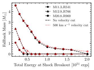
Figure 29: Mass of fallback material at shock breakout as a function of the total energy of the exploded model at the time of shock breakout for three different progenitor models exploded with 12 different explosion energies. Results are shown for the new integrated energy fallback criterion with no additional velocity cut (black points), and the same criterion with a 500 km s^-1 velocity cut at shock breakout (red points).

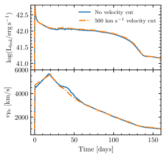
Figure 30: Effects of a velocity cut on STELLA light curves and Fe II 5169Å line velocities for our M12.9_R766 progenitor model exploded with $E_{\rm tot}=5.0\times 10^{51}$ ergs and a nickel mass $M_{\rm Ni}=0.042M_{\odot}$, where we see a noticeable difference between the mass of fallback material with and without a velocity cut ($\approx 0.3M_{\odot}$).

Appendix B Extension of the Plateau due to ${{}^{56}{\rm Ni}}$ Decay

We start with the thermodynamic equation, where a fluid is heated by nuclear decay (in our case, of ${{}^{56}{\rm Ni}}$) with complete trapping

$$TdS=dE+PdV=L_{\rm nuc}dt$$ (B1)

In a 1-zone, radiation-dominated regime, we can express $P=E/3V$ and $V=4\pi(vt)^{3}/3$. Assuming homology, $dV/V=3dt/t$, and this becomes

$$\frac{1}{t}d(Et)=L_{\rm nuc}dt.$$ (B2)

To find the total energy at time $t$, integrate from from $t_{\rm SB}$ to obtain:

$$E(t)=E_{0}\frac{t_{\rm SB}}{t}+\frac{1}{t}\int_{t_{\rm SB}}^{t}t^{\prime}L_{\rm nuc}\,dt^{\prime},$$ (B3)

where $L_{\rm nuc}$ is due to the ${{}^{56}{\rm Ni}}\rightarrow{{}^{56}{\rm Co}}\rightarrow{{}^{56}{\rm Fe}}$ decay chain, following Nadyozhin (1994):

$$L_{\rm nuc}=\frac{N_{\rm Ni}Q_{\rm Ni}}{\tau_{\rm Ni}}\exp\left(\frac{-t}{\tau_{\rm Ni}}\right)+\frac{N_{\rm Ni}Q_{\rm Co}}{\tau_{\rm Co}-\tau_{\rm Ni}}\left[\exp\left(\frac{-t}{\tau_{\rm Co}}\right)-\exp\left(\frac{-t}{\tau_{\rm Ni}}\right)\right],$$ (B4)

where $N_{\rm Ni}=M_{{\rm Ni}}/(56\,{\rm amu})$, $\tau_{\rm X}$ is the lifetime of radioactive species X, and $Q_{\rm X}$ is the energy per decay of species X.

Assuming only ${{}^{56}{\rm Ni}}$ is produced in the explosion and all ${{}^{56}{\rm Co}}$ comes from ${{}^{56}{\rm Ni}}$ decay, the contribution to the internal energy due to the ${{}^{56}{\rm Ni}}$ decay chain over the lifetime of the SN is

$$E_{\rm tot,Ni}=\frac{1}{t_{\rm p}}\int_{t_{\rm SB}}^{t_{\rm p}}tL_{\rm nuc}\,dt.$$ (B5)

We now make a few approximations: First, by the end of the plateau, ${{}^{56}{\rm Ni}}$ has undergone many decay times. Thus we take $t_{\rm SB}\rightarrow 0$ and $t_{\rm p}/\tau_{\rm Ni}\rightarrow\infty$ when in the bounds of our integrals. However, the decay time of ⁵⁶Co is 111.3 days, which is comparable to $t_{\rm p}$. Thus we approximate $t_{\rm p}/\tau_{\rm Co}\approx 1$ when in the bounds of our integrals. Outside the integrals, we assume that the time to shock breakout is roughly the expansion time, $t_{\rm SB}\approx t_{\rm e}$, where, as in Section 3,

$$t_{\rm e} =R_{0}/v_{\rm e},$$

$$v_{\rm e} =\sqrt{\frac{2E_{\rm exp}}{M_{\rm ej}}}\approx 3.16\times 10^{8}M_{10}E_{51}\mathrm{\ cm\ s^{-1}}.$$

Any numerical quantities are, in reality, dependent on the specifics of the relevant timescales. Here we aim primarily to capture the relevant scaling relationships, fitting against our models to find appropriate numerical prefactors.

Computing these integrals and simplifying, we find that

$$E_{\rm int}(t_{\rm p}) =\frac{E_{0}\,t_{e}}{t_{\rm p}}+\frac{N_{\rm Ni}}{t_{\rm p}}\left[Q_{\rm Ni}\tau_{\rm Ni}+Q_{\rm Co}\left(\frac{0.26\tau_{\rm Co}^{2}-\tau_{\rm Ni}^{2}}{\tau_{\rm Co}-\tau_{\rm Ni}}\right)\right]$$ (B6)

$$=\frac{E_{0}\,t_{e}}{t_{\rm p}}\times f_{\rm rad},\ {\rm where}$$ (B7)

$$f_{\rm rad} \equiv 1+\frac{N_{\rm Ni}}{t_{e}E_{0}}\left(Q_{\rm Ni}\tau_{\rm Ni}+Q_{\rm Co}\tau^{\prime}_{\rm Co}\right)\ {\rm and}$$ (B8)

$$\tau^{\prime}_{\rm Co} \equiv\left(\frac{0.26\tau_{\rm Co}^{2}-\tau_{\rm Ni}^{2}}{\tau_{\rm Co}-\tau_{\rm Ni}}\right),$$ (B9)

noting that $E_{0},$ the internal energy at $t_{\rm SB}$, is roughly half the total energy of the explosion (mentioned as a comment in K&W), we set $E_{0}=E_{\rm exp}/2$.

We can re-express $f_{\rm rad}$ as

$$f_{\rm rad}=1+\frac{M_{\rm Ni}}{E_{0}}\frac{\tau_{\rm Ni}}{t_{e}}\left(q_{\rm Ni}+q_{\rm Co}\frac{\tau^{\prime}_{\rm Co}}{\tau_{\rm Ni}}\right)$$ (B10)

where $q_{\rm X}$ is the specific (per gram) energy released by the decay of species X; in this case $q_{\rm X}=Q_{\rm X}/56\,{\rm amu}$.

Following Nadyozhin (1994), we use $Q_{\rm Ni}=1.75$ MeV/nucleon, $Q_{\rm Co}=3.73$ MeV/nucleon, $\tau_{\rm Ni}=8.8$ days, and $\tau_{\rm Co}=111.3$ days. We thus find that

$$f_{\rm rad}\approx 1+7.0\left(M_{{\rm Ni},\odot}\,E_{51}^{-1/2}\,R_{500}^{-1}\,M_{10}^{-1/2}\right).$$ (B11)

This argument ignores the effects of the distribution of ${{}^{56}{\rm Ni}}$, as we necessarily have assumed in this simple 1-zone model that the nickel is distributed evenly throughout the ejecta. If the heat from the ${{}^{56}{\rm Ni}}$ decay is trapped inside the core of the star until that material becomes optically thin, then this would further extend the duration of the plateau. Thus, we should treat the factor of 7.0 as a rough lower bound, rather than an expectation.

We can also recast Equation (B11) in terms of $ET$ and $\eta_{\rm Ni}$. Although our derivation assumes all internal energy is trapped to be radiated away, and the Shussman et al. (2016a) derivation of $ET$ assumes that all energy is radiated away, this is just a difference in terms and not a difference in physics. Thus at $t=t_{\rm p}$, plugging in $ET=E_{0}t_{\rm SB}\approx E_{0}t_{e}$ and $\eta_{\rm Ni}=\left(\int_{t_{\rm SB}}^{t_{\rm p}}tL_{\rm nuc}\,dt\right)/ET$ to Equation (B3), we recover

$$E_{\rm int}(t_{\rm p})=E_{0}\frac{t_{e}}{t_{\rm p}}+\frac{ET\,\eta_{\rm Ni}}{t_{\rm p}}\approx\frac{E_{0}\,t_{e}}{t_{\rm p}}(1+\eta_{\rm Ni}),$$ (B12)

so $f_{\rm rad}\approx 1+\eta_{\rm Ni}$.

References

- Arnett (1980) Arnett, W. D. 1980, ApJ, 237, 541
- Baklanov et al. (2005) Baklanov, P. V., Blinnikov, S. I., & Pavlyuk, N. N. 2005, Astronomy Letters, 31, 429
- Bellm et al. (2019) Bellm, E. C., Kulkarni, S. R., Graham, M. J., et al. 2019, PASP, 131, 018002
- Bersten & Hamuy (2009) Bersten, M. C., & Hamuy, M. 2009, ApJ, 701, 200
- Blinnikov & Sorokina (2004) Blinnikov, S., & Sorokina, E. 2004, Ap&SS, 290, 13
- Blinnikov et al. (1998) Blinnikov, S. I., Eastman, R., Bartunov, O. S., Popolitov, V. A., & Woosley, S. E. 1998, ApJ, 496, 454
- Blinnikov et al. (2006) Blinnikov, S. I., Röpke, F. K., Sorokina, E. I., et al. 2006, A&A, 453, 229
- Brayton et al. (1972) Brayton, R. K., Gustavson, F. G., & Hachtel, G. D. 1972, Proceedings of the IEEE, 60, 98
- Brown et al. (2013) Brown, T. M., Baliber, N., Bianco, F. B., et al. 2013, PASP, 125, 1031
- Burrows et al. (2019) Burrows, A., Radice, D., & Vartanyan, D. 2019, MNRAS, 538
- Castor (1970) Castor, J. I. 1970, MNRAS, 149, 111
- Chugai (1991) Chugai, N. N. 1991, Soviet Astronomy Letters, 17, 210
- Dessart & Hillier (2019) Dessart, L., & Hillier, D. J. 2019, arXiv e-prints, arXiv:1903.04840
- Dessart et al. (2013) Dessart, L., Hillier, D. J., Waldman, R., & Livne, E. 2013, MNRAS, 433, 1745
- Duffell (2016) Duffell, P. C. 2016, ApJ, 821, 76
- Gear (1971) Gear, C. W. 1971, Numerical initial value problems in ordinary differential equations, Prentice-Hall Series in Automatic Computation (Prentice-Hall, Engelwood Cliffs)
- Gutiérrez et al. (2017) Gutiérrez, C. P., Anderson, J. P., Hamuy, M., et al. 2017, ApJ, 850, 90
- Hamuy (2003) Hamuy, M. 2003, ApJ, 582, 905
- Hunter (2007) Hunter, J. D. 2007, Computing In Science & Engineering, 9, 90
- Jerkstrand et al. (2012) Jerkstrand, A., Fransson, C., Maguire, K., et al. 2012, A&A, 546, A28
- Jones et al. (2001–) Jones, E., Oliphant, T., Peterson, P., et al. 2001–, SciPy: Open source scientific tools for Python
- Kasen et al. (2006) Kasen, D., Thomas, R. C., & Nugent, P. 2006, ApJ, 651, 366
- Kasen & Woosley (2009) Kasen, D., & Woosley, S. E. 2009, ApJ, 703, 2205
- Kluyver et al. (2016) Kluyver, T., Ragan-Kelley, B., Pérez, F., et al. 2016, in Positioning and Power in Academic Publishing: Players, Agents and Agendas: Proceedings of the 20th International Conference on Electronic Publishing, IOS Press, 87
- Kochanek et al. (2017) Kochanek, C. S., Shappee, B. J., Stanek, K. Z., et al. 2017, Publications of the Astronomical Society of the Pacific, 129, 104502
- Kozyreva et al. (2018) Kozyreva, A., Nakar, E., & Waldman, R. 2018, MNRAS, 483, 1211
- Lisakov et al. (2017) Lisakov, S. M., Dessart, L., Hillier, D. J., Waldman, R., & Livne, E. 2017, MNRAS, 466, 34
- Litvinova & Nadyozhin (1983) Litvinova, I. Y., & Nadyozhin, D. K. 1983, Astrophysics and Space Science, 89, 89
- LSST Science Collaboration et al. (2009) LSST Science Collaboration, Abell, P. A., Allison, J., et al. 2009, arXiv e-prints, arXiv:0912.0201 [astro-ph.IM]
- Mihalas (1978) Mihalas, D. 1978, Stellar atmospheres /2nd edition/
- Morozova et al. (2016) Morozova, V., Piro, A. L., Renzo, M., & Ott, C. D. 2016, ApJ, 829, 109
- Morozova et al. (2017) Morozova, V., Piro, A. L., & Valenti, S. 2017, ApJ, 838, 28
- Müller et al. (2017) Müller, T., Prieto, J. L., Pejcha, O., & Clocchiatti, A. 2017, ApJ, 841, 127
- Nadyozhin (1994) Nadyozhin, D. K. 1994, ApJS, 92, 527
- Nakar et al. (2016) Nakar, E., Poznanski, D., & Katz, B. 2016, ApJ, 823, 127
- Paxton et al. (2011) Paxton, B., Bildsten, L., Dotter, A., et al. 2011, ApJS, 192, 3
- Paxton et al. (2013) Paxton, B., Cantiello, M., Arras, P., et al. 2013, ApJS, 208, 4
- Paxton et al. (2015) Paxton, B., Marchant, P., Schwab, J., et al. 2015, ApJS, 220, 15
- Paxton et al. (2018) Paxton, B., Schwab, J., Bauer, E. B., et al. 2018, ApJS, 234, 34
- Paxton et al. (2019) Paxton, B., Smolec, R., Gautschy, A., et al. 2019, arXiv e-prints, arXiv:1903.01426
- Pejcha & Prieto (2015a) Pejcha, O., & Prieto, J. L. 2015a, ApJ, 799, 215
- Pejcha & Prieto (2015b) —. 2015b, ApJ, 806, 225
- Pérez & Granger (2007) Pérez, F., & Granger, B. E. 2007, Computing in Science & Engineering, 9, 21
- Perna et al. (2014) Perna, R., Duffell, P., Cantiello, M., & MacFadyen, A. I. 2014, ApJ, 781, 119
- Popov (1993) Popov, D. V. 1993, ApJ, 414, 712
- Shussman et al. (2016a) Shussman, T., Nakar, E., Waldman, R., & Katz, B. 2016a, arXiv e-prints, arXiv:1602.02774 [astro-ph.HE]
- Shussman et al. (2016b) Shussman, T., Waldman, R., & Nakar, E. 2016b, arXiv e-prints, arXiv:1610.05323 [astro-ph.HE]
- Smartt (2009) Smartt, S. J. 2009, ARA&A, 47, 63
- Smartt (2015) —. 2015, Publications of the Astronomical Society of Australia, 32, e016
- Sobolev (1960) Sobolev, V. V. 1960, Moving envelopes of stars
- Sukhbold et al. (2016) Sukhbold, T., Ertl, T., Woosley, S. E., Brown, J. M., & Janka, H.-T. 2016, ApJ, 821, 38
- Utrobin (2007) Utrobin, V. P. 2007, A&A, 461, 233
- Utrobin et al. (2017) Utrobin, V. P., Wongwathanarat, A., Janka, H.-T., & Müller, E. 2017, ApJ, 846, 37
- Valenti et al. (2016) Valenti, S., Howell, D. A., Stritzinger, M. D., et al. 2016, MNRAS, 459, 3939
- van der Walt et al. (2011) van der Walt, S., Colbert, S. C., & Varoquaux, G. 2011, Computing in Science Engineering, 13, 22
- Wolf et al. (2017) Wolf, B., Bauer, E. B., & Schwab, J. 2017, wmwolf/MesaScript: A DSL for Writing MESA Inlists
- Wolf & Schwab (2017) Wolf, B., & Schwab, J. 2017, wmwolf/py_mesa_reader: Interact with MESA Output
- Wongwathanarat et al. (2015) Wongwathanarat, A., Müller, E., & Janka, H.-T. 2015, A&A, 577, A48
- Woosley & Weaver (1988) Woosley, S. E., & Weaver, T. A. 1988, Phys. Rep., 163, 79