Remarks on the scale invariant Cassinian metric

Abstract.

We study the geometry of the scale invariant Cassinian metric and prove sharp comparison inequalities between this metric and the hyperbolic metric in the case when the domain is either the unit ball or the upper half space. We also prove sharp distortion inequalities for the scale invariant Cassinian metric under Möbius transformations.

Keywords. the scale invariant Cassinian metric, the hyperbolic metric, Möbius transformation

2010 Mathematics Subject Classification. 30F45 (51M10)

1. Introduction

In the Euclidean space ${\mathbb{R}^{n}},n\geq 2\,,$ the natural way to measure distance between two points $x,y\in{\mathbb{R}^{n}}$ is to use the length $|x-y|$ of the segment joining the points. In geometric function theory [6], one studies functions defined in subdomains $D\subset{\mathbb{R}^{n}}\,,$ and measures distances between two points $x,y\in D\,.$ In this case the Euclidean distance is no longer an adequate method for measuring the distance, because one has to take into account also the position of the points relative to the boundary $\partial D\,.$

During the past few decades, many authors have suggested metrics for this purpose. In the case of the simplest domain, the unit ball ${\mathbb{B}^{n}}\,,$ we have the hyperbolic or Poincaré metric that is the most common metric in this case. Therefore, it is a natural idea to analyze the various equivalent definitions of the hyperbolic metric and to use these to generalize, if possible, the hyperbolic metric to the case of a given domain $D\subset{\mathbb{R}^{n}}\,.$ These generalizations capture usually some but not all features of the hyperbolic metric and are thus called hyperbolic type metrics [3, 5, 7, 9, 10, 12, 13, 15, 16, 20].

Because the usefulness of a metric depends on how well its invariance properties match those of the function spaces studied, we now analyze hyperbolic type metrics from this point of view. The best we can expect is invariance in the same sense as the hyperbolic metrics are invariant, namely invariance under Möbius transformations of the Möbius space $(\overline{\mathbb{R}}^{n},q)\,,\overline{\mathbb{R}}^{n}={\mathbb{R}}^{n}\cup\{\infty\}\,,$ equipped with the chordal metric $q\,.$ Another useful notion is invariance with respect to similarity transformations. A similarity transformation is a transformation of the form $x\mapsto\lambda U(x)+b$ where $\lambda>0\,,$ $b\in\mathbb{R}^{n}\,,$ and $U$ is an orthogonal map, i.e., a linear map with $|U(x)|=|x|$ for all $x\in\mathbb{R}^{n}\,.$

The quasihyperbolic and the distance ratio metrics introduced by Gehring and Palka [7] have become widely used hyperbolic type metrics in geometric function theory in plane and space [6]. Both metrics are defined for subdomains of ${\mathbb{R}}^{n}\,$ and are invariant under similarity transformations, but they are not Möbius invariant. Möbius invariant metrics, defined in terms of the absolute ratios of quadruples of points, were studied by several authors in the case of a general domain $D\subset\overline{\mathbb{R}}^{n}$ with ${\rm card}(\overline{\mathbb{R}}^{n}\setminus D)\geq 2\,.$ These metrics include the Apollonian metric of Beardon [3], the Möbius invariant metric of Seittenranta [20], and the generalized hyperbolic metric of Hästö [10]. Each of these metrics generates its own geometry and the study of transformation rules of these metrics under Möbius transformations and conformal mappings are natural questions to study. If we can describe the balls of a metric space ”explicitly”, then we already know a lot about the geometry of the metric – this requires that we can estimate the metric in terms of well-known metrics. For a survey and comparison inequalities between some of these metrics, see [4, 8, 11, 18, 19, 20, 22, 23].

Recently Ibragimov [13] introduced the scale invariant Cassinian metric $\tilde{\tau}_{D}$, see the definition below in 2.14. It is readily seen that the metric $\tilde{\tau}_{D}$ is invariant under similarity transformations. Several authors [13, 18, 19] have studied some basic properties of the scale invariant Cassinian metric and its distortion under Möbius transformations of the unit ball, and also quasi-invariance properties under quasiconformal mappings.

In this paper, we will continue this research and study the geometry of the scale invariant Cassinian metric and establish sharp comparison results between this metric and the hyperbolic metric of the unit ball or of the upper half space, and also prove sharp distortion inequalities under Möbius transformations.

2. Preliminaries

2.1.

Hyperbolic metric. The hyperbolic metric $\rho_{\mathbb{B}^{n}}$ and $\rho_{\mathbb{H}^{n}}$ of the unit ball ${\mathbb{B}^{n}}=\{z\in{\mathbb{R}^{n}}:|z|<1\}$ and of the upper half space ${\mathbb{H}^{n}}=\{(x_{1},\ldots,x_{n})\in{\mathbb{R}^{n}}:x_{n}>0\}$ can be defined as follows. By [2, p.40] we have for $x,y\in\mathbb{B}^{n}$ ,

(2.2) $$\,\textnormal{sh}{\frac{\rho_{\mathbb{B}^{n}}(x,y)}{2}}=\frac{|x-y|}{\sqrt{1-|x|^{2}}{\sqrt{1-|y|^{2}}}}\,,$$

and by [2, p.35] for $x,y\in\mathbb{H}^{n}$ ,

(2.3) $$\,\textnormal{ch}{\rho_{\mathbb{H}^{n}}(x,y)}=1+\frac{|x-y|^{2}}{2x_{n}y_{n}}\,.$$

Two special formulas of the hyperbolic metric are frequently used [21, (2.17),(2.6)] :

(2.4) $$\rho_{\mathbb{B}^{n}}(re_{1},se_{1})=\log\left(\frac{1+s}{1-s}\cdot\frac{1-r}{1+r}\right)\,,\quad{\rm for}\quad-1<r<s<1\,,\quad s>0\,,$$

and

(2.5) $$\rho_{\mathbb{H}^{n}}(re_{n},se_{n})=\log\frac{s}{r}\,,\quad{\rm for}\quad 0<r<s\,.$$

2.6.

Absolute ratio. For a quadruple of distinct points $a,b,c,d,\in\overline{\mathbb{R}}^{n}$ , the absolute ratio is defined as

$$|a,b,c,d|=\frac{q(a,c)q(b,d)}{q(a,b)q(c,d)}\,,$$

where $q(a,c)$ is the chordal distance [21, (1.14)]. The most important property of the absolute ratio is its invariance under Möbius transformations [2, Theorem 3.2.7]. For the basic properties of Möbius transformations the reader is referred to [2] .

In terms of the absolute ratio, the hyperbolic metric $\rho_{D}\,,$ $D\in\{\mathbb{B}^{n},\mathbb{H}^{n}\}\,,$ can be defined for $x,y\in D$ as follows [2, (7.26)] :

(2.7) $$\rho_{D}(x,y)=\sup\{\log|u,x,y,v|:u,v\in\partial D\}\,.$$

Because of the Möbius invariance of the absolute ratio and (2.7) , we may define for every Möbius transformation $g$ the hyperbolic metric in $g(\mathbb{B}^{n})$. This metric will be denoted by $\rho_{g(\mathbb{B}^{n})}$. In particular, if $g:{\mathbb{B}^{n}}\to{\mathbb{H}^{n}}$ is a Möbius transformation with $g({\mathbb{B}^{n}})={\mathbb{H}^{n}},$ then for all $x,y\in{\mathbb{B}^{n}}$ there holds $\rho_{\mathbb{B}^{n}}(x,y)=\rho_{\mathbb{H}^{n}}(g(x),g(y))\,.$

2.8.

Distance ratio metric. For a proper open subset $D$ of $\mathbb{R}^{n}$ and for $x,y\in D$, the distance ratio metric $j_{D}$ is defined as

$$j_{D}(x,y)=\log\left(1+\frac{|x-y|}{\min\{d(x,\partial D),d(y,\partial D)\}}\right)\,,$$

where $d(x,\partial D)$ denotes the Euclidean distance from the point $x$ to the boundary $\partial D$. The distance ratio metric was introduced by Gehring and Palka [7] and in the above simplified form by Vuorinen [21, (2.34)].

The well-known relation between the distance ratio metric and the hyperbolic metric is shown in the following lemma.

Lemma 2.9.

[1, Lemma 7.56], [21, Lemma 2.41(2)] Let $D\in\{\mathbb{B}^{n},\mathbb{H}^{n}\}$. Then for all $x,y\in D$, we have

$$\frac{1}{2}\rho_{D}(x,y)\leq j_{D}(x,y)\leq\rho_{D}(x,y)\,.$$

2.10.

Cassinian oval. A Cassinian oval $C(\alpha_{1},\alpha_{2};b)$ is defined as

$$\{z\in\mathbb{R}^{2}:|z-\alpha_{1}|\cdot|z-\alpha_{2}|=b^{2}\}\,,$$

where $b>0$ and $\alpha_{1}$, $\alpha_{2}$ are two fixed points called the foci of the oval.

Let $\alpha_{1}=(-a,0)$ and $\alpha_{2}=(a,0)$ with $a\in{\mathbb{R}}$ , then the equation of the Cassinian oval $C(\alpha_{1},\alpha_{2};b)$ is

(2.11) $$\left((z_{1}-a)^{2}+z_{2}^{2}\right)\left((z_{1}+a)^{2}+z_{2}^{2}\right)=b^{4}\,.$$

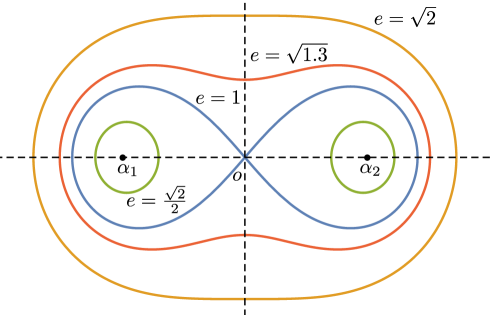
Figure 1. Cassinian ovals with $e=\frac{\sqrt{2}}{2}$, $e=1$, $e=\sqrt{1.3}$, and $e=\sqrt{2}$, respectively.

The shape of a Cassinian oval depends on $e=\frac{b}{a}$ (see Fig.1). When $e<1$, the oval consists of two separate loops . When $e=1$, the oval is the lemniscate of Bernoulli having the shape of number eight . When $e>1$, the oval is a single loop enclosing both foci. Moreover, it is peanut-shaped for $1<e<\sqrt{2}$ and convex for $e\geq\sqrt{2}$. In the limiting case $a\rightarrow 0$ the Cassinian oval reduces to a circle.

Proposition 2.12.

Let $p=(p_{1},p_{2})$ be a point on the Cassinian oval $C(\alpha_{1},\alpha_{2};b)$. Then the distance from the origin to the point $p$ is increasing as a function of $p_{1}>0$.

Proof.

By (2.11), we have

$$|p|^{2}=p_{1}^{2}+p_{2}^{2}=\sqrt{4a^{2}p_{1}^{2}+b^{4}}-a^{2},$$

which implies that the distance from the origin to the point $p$ is increasing for $p_{1}>0$ . ∎

Proposition 2.13.

The Cassinian oval $C(\alpha_{1},\alpha_{2};b)$ inscribes the circle $\partial{\mathbb{B}^{2}}(\sqrt{a^{2}+b^{2}})$ .

Proof.

By Proposition 2.12 and (2.11), it is clear that the maximum distance from the origin to the point $p$ on the Cassinian oval $C(\alpha_{1},\alpha_{2};b)$ is $\sqrt{a^{2}+b^{2}}$ . ∎

2.14.

Scale invariant Cassinian metric. For a proper subdomain $D$ of $\mathbb{R}^{n}$ and for all $x,y\in D$, the scale invariant Cassinian metric $\tilde{\tau}_{D}$ is defined as [13]

$$\tilde{\tau}_{D}(x,y)=\log\left(1+\sup_{p\in\partial D}\frac{|x-y|}{\sqrt{|x-p||y-p|}}\right).$$

Geometrically, $\tilde{\tau}_{D}(x,y)$ can be defined by means of the maximal Cassinian oval $C\subset\overline{D}$ with foci $x,y\in D$. Then for every point $p\in C$, we have

$$\tilde{\tau}_{D}(x,y)=\log\left(1+\frac{|x-y|}{\sqrt{|x-p||y-p|}}\right).$$

Because of this geometric interpretation, the metric $\tilde{\tau}_{D}$ is monotonic with respect to domains, i.e., if $D\subset D^{\prime}$, then $\tilde{\tau}_{D^{\prime}}(x,y)\leq\tilde{\tau}_{D}(x,y)$ for $x\,,y\in D$.

The following lemma shows the relation between the scale invariant Cassinian metric and the distance ratio metric.

Lemma 2.15.

[13, Theorem 3.3] Let $D\subset\mathbb{R}^{n}$ be a domain with $\partial D\neq\emptyset$. For all $x,y\in D$, we have

$$\frac{1}{2}j_{D}(x,y)\leq\tilde{\tau}_{D}(x,y)\leq j_{D}(x,y)$$

and

$$\tilde{\tau}_{D}(x,y)\leq\frac{1}{2}j_{D}(x,y)+\frac{1}{2}\log 3\,.$$

All the inequalities are sharp.

2.16.

Möbius invariant Cassinian metric. Let $D$ be a subdomain of $\overline{\mathbb{R}}^{n}$ with ${\rm card}(\partial D)\geq 2$. For $x,y\in D$, the Möbius invariant Cassinian metric $\tau_{D}$ is defined as [15]

$$\tau_{D}(x,y)=\log\left(1+\sup_{p,q\in\partial D}\frac{|x-y||p-q|}{\sqrt{|x-p||y-q||x-q||y-p|}}\right).$$

Since $\tau_{D}$ can be expressed as

$$\tau_{D}(x,y)=\log\left(1+\sup_{p,q\in\partial D}\sqrt{\frac{|x-y||p-q|}{|x-p||y-q|}}\sqrt{\frac{|x-y||q-p|}{|x-q||y-p|}}\right)\,,$$

the Möbius invariant Cassinian metric is Möbius invariant. Namely,

Lemma 2.17.

[15, Corollary 2.1] Let $f$ be a Möbius transformation of $\overline{\mathbb{R}}^{n}$ and $D\subset\overline{\mathbb{R}}^{n}$ with ${\rm card}(\partial D)\geq 2$. Then for all $x,y\in D$, we have

$$\tau_{f(D)}\left(f(x),f(y)\right)=\tau_{D}(x,y)\,.$$

The following lemma shows the relation between the scale invariant Cassinian metric and the Möbius invariant Cassinian metric.

Lemma 2.18.

[15, Theorem 3.3] For all $x,y\in D\subsetneq\mathbb{R}^{n}$, we have

$$\frac{1}{2}\tau_{D}(x,y)\leq\tilde{\tau}_{D}(x,y)\leq\tau_{D}(x,y)\,.$$

3. The estimate of $\tilde{\tau}$-metric

In this section, we give the estimate for the scale invariant Cassinian metric in the unit disk or the upper half plane by studying the formulas of special cases and the geometry of the $\tilde{\tau}$-metric. The results can be applied to higher-dimensional cases, e.g., the special formulas are used in the proof of the results in Sections 4 and 5. For the convenience, we identify ${\mathbb{R}}^{2}$ with the complex plane $\mathbb{C}$ and use complex number notation also if needed in the sequel.

3.1.

The unit disk case. We first study the formulas of special cases of the scale invariant Cassinian metric in the unit disk.

Lemma 3.2.

Let $x,y\in\mathbb{B}^{2}\setminus\{0\}$ with $|x|=|y|$.

(1) If $|x+y|\leq\frac{4|x|^{2}}{1+|x|^{2}}$, then

$$\tilde{\tau}_{\mathbb{B}^{2}}(x,y)=\log\left(1+\sqrt{\frac{2|x||x-y|}{1-|x|^{2}}}\right).$$

(2) If $|x+y|>\frac{4|x|^{2}}{1+|x|^{2}}$, then

$$\tilde{\tau}_{\mathbb{B}^{2}}(x,y)=\log\left(1+\frac{|x-y|}{\sqrt{1+|x|^{2}-|x+y|}}\right).$$

Proof.

By symmetry, we may assume that $x=(x_{1},x_{2})$ and $y=(x_{1},-x_{2})$, where $x_{1}=\frac{|x+y|}{2},~{}x_{2}=\frac{|x-y|}{2}$. Let $p=(t,\sqrt{1-t^{2}})$ with $x_{1}\leq t\leq 1$ and

$$f(t) =|x-p|^{2}|y-p|^{2}$$

$$=\left((x_{1}^{2}+x_{2}^{2}+1-2x_{1}t)-2x_{2}\sqrt{1-t^{2}}\right)\left((x_{1}^{2}+x_{2}^{2}+1-2x_{1}t)+2x_{2}\sqrt{1-t^{2}}\right)$$

$$=4(x_{1}^{2}+x_{2}^{2})t^{2}-4x_{1}(x_{1}^{2}+x_{2}^{2}+1)t+(x_{1}^{2}+x_{2}^{2})^{2}+2x_{1}^{2}-2x_{2}^{2}+1\,.$$

(1) If $|x+y|\leq\frac{4|x|^{2}}{1+|x|^{2}}$, then

$$f_{\min}(t)=f(t_{0})=\frac{x_{2}^{2}(1-x_{1}^{2}-x_{2}^{2})^{2}}{x_{1}^{2}+x_{2}^{2}}\,,$$

where $t_{0}=\frac{x_{1}}{2}(1+\frac{1}{x_{1}^{2}+x_{2}^{2}})\,.$ Therefore,

$$\tilde{\tau}_{\mathbb{B}^{2}}(x,y)=\log\left(1+\frac{|x-y|}{\sqrt[4]{f(t_{0})}}\right)=\log\left(1+\sqrt{\frac{2|x||x-y|}{1-|x|^{2}}}\right)\,.$$

(2) If $|x+y|>\frac{4|x|^{2}}{1+|x|^{2}}$, then

$$f_{\min}(t)=f(1)\,.$$

Therefore,

$$\tilde{\tau}_{\mathbb{B}^{2}}(x,y)=\log\left(1+\frac{|x-y|}{\sqrt[4]{f(1)}}\right)=\log\left(1+\frac{|x-y|}{\sqrt{1+|x|^{2}-|x+y|}}\right).$$

This completes the proof. ∎

Lemma 3.3.

[18, Proposition 3.1] Let $x,y\in\mathbb{B}^{2}$ with $x~{}=~{}ty$, $t\in\mathbb{R}\setminus\{0\}$ and $|x|\leq|y|$.

(1) If $t>0$, then

$$\tilde{\tau}_{\mathbb{B}^{2}}(x,y)=\log\left(1+\frac{|x-y|}{\sqrt{(1-|x|)(1-|y|)}}\right).$$

(2) If $t<0$, then

$$\tilde{\tau}_{\mathbb{B}^{2}}(x,y)=\log\left(1+\frac{|x-y|}{\sqrt{(1+|x|)(1-|y|)}}\right).$$

Remark 3.4.

By definition, it is easy to see that

$$\tilde{\tau}_{\mathbb{B}^{2}}(0,x)=\log\left(1+\frac{|x|}{\sqrt{1-|x|}}\right).$$

Lemma 3.5.

$Let~{}x,y,x^{\prime},y^{\prime}\in\mathbb{B}^{2}$ with $x^{\prime}=\frac{x+y}{2}-\frac{|x-y|}{2}\xi$, $y^{\prime}=\frac{x+y}{2}+\frac{|x-y|}{2}\xi$,  $x^{\prime\prime}=\frac{x+y}{2}-\frac{|x-y|}{2}\zeta$ and $y^{\prime\prime}=\frac{x+y}{2}+\frac{|x-y|}{2}\zeta$ , where

$$\xi=\left\{\begin{array}[]{ll}\frac{x+y}{|x+y|},&x+y\neq 0\,,\\ e_{1},&x+y=0\,,\end{array}\right.$$

and $\zeta=i\,\xi$ . Then

$$\tilde{\tau}_{\mathbb{B}^{2}}(x^{\prime\prime},y^{\prime\prime})\leq\tilde{\tau}_{\mathbb{B}^{2}}(x,y)\leq\tilde{\tau}_{\mathbb{B}^{2}}(x^{\prime},y^{\prime})\,.$$

Proof.

Since the result is trivially true for the case $x=-y$, by symmetry, we may assume that $x\neq-y$ and $0<\arg\frac{y-x}{y+x}<\frac{\pi}{2}$.

Let $b^{\prime}\in\mathbb{R}$ such that $C(x^{\prime},y^{\prime};b^{\prime})$ is tangent to $\partial\mathbb{B}^{2}$ at $\xi$. By Proposition 2.13, there exists a disk $\mathbb{B}^{2}(o^{\prime},r)\subset\mathbb{B}^{2}$ such that $C(x^{\prime},y^{\prime};b^{\prime})$ inscribes $\overline{\mathbb{B}^{2}}(o^{\prime},r)$, where the center $o^{\prime}=\frac{x+y}{2}$ and the radius $r=\sqrt{b^{\prime 2}+\frac{|x-y|^{2}}{4}}$. Moreover, $C(x^{\prime},y^{\prime};b^{\prime})\cap\partial\mathbb{B}^{2}(o^{\prime},r)\cap\partial\mathbb{B}^{2}$ has one and only one point.

With rotation, $C(x,y;b^{\prime})\subsetneq\mathbb{B}^{2}$ (see Fig. 3). Therefore, there exists a positive number $b\,(>b^{\prime})$ such that $C(x,y;b)$ is tangent to $\partial\mathbb{B}^{2}$ . Hence

$$\tilde{\tau}_{\mathbb{B}^{2}}(x,y)\leq\tilde{\tau}_{\mathbb{B}^{2}}(x^{\prime},y^{\prime})\,.$$

With rotation and by Proposition 2.12, $C(x^{\prime\prime},y^{\prime\prime};b)\subsetneq\mathbb{B}^{2}$ (see Fig. 3). Therefore, there exists a positive number $b^{\prime\prime}\,(>b)$ such that $C(x^{\prime\prime},y^{\prime\prime};b^{\prime\prime})$ is tangent to $\partial\mathbb{B}^{2}$ . Hence

$$\tilde{\tau}_{\mathbb{B}^{2}}(x^{\prime\prime},y^{\prime\prime})\leq\tilde{\tau}_{\mathbb{B}^{2}}(x,y)\,.$$

This completes the proof. ∎

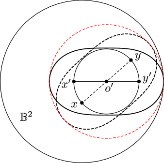
Figure 2. The Cassinian oval $C(x^{\prime},y^{\prime};b^{\prime})$ is tangent to $\partial\mathbb{B}^{2}$ while $C(x,y;b^{\prime})\subsetneq\mathbb{B}^{2}$.

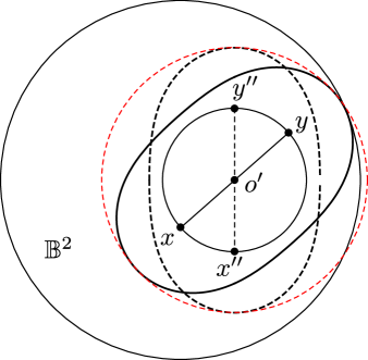
Figure 3. The Cassinian oval $C(x,y;b)$ is tangent to $\partial\mathbb{B}^{2}$ while $C(x^{\prime\prime},y^{\prime\prime};b)\subsetneq\mathbb{B}^{2}$.

Theorem 3.6.

For $x,y\in\mathbb{B}^{2}$, we have

(3.9) $$\tilde{\tau}_{\mathbb{B}^{2}}(x,y)\geq\left\{\begin{array}[]{ll}\log\left(1+2\sqrt{\frac{|x-y|\sqrt{|x+y|^{2}+|x-y|^{2}}}{4-|x+y|^{2}-|x-y|^{2}}}\right),&|x+y|\left(1+\frac{4}{|x+y|^{2}+|x-y|^{2}}\right)\leq 4\,,\\ \log\left(1+\frac{2|x-y|}{\sqrt{(2-|x+y|)^{2}+|x-y|^{2}}}\right),&|x+y|\left(1+\frac{4}{|x+y|^{2}+|x-y|^{2}}\right)>4,\end{array}\right.$$

and

(3.10) $$\tilde{\tau}_{\mathbb{B}^{2}}(x,y)\leq\log\left(1+\frac{2|x-y|}{\sqrt{(2-|x+y|)^{2}-|x-y|^{2}}}\right),\quad|x+y|+|x-y|<2\,.$$

Proof.

Since the equalities in (3.9) and (3.10) clearly hold when $x=-y$, we may assume that $x\neq-y$ in the sequel.

To prove inequalities (3.9), let $x^{\prime\prime}\,,y^{\prime\prime}$ be the same as in Lemma 3.5. Then

$$x^{\prime\prime}=\frac{x+y}{2\,|x+y|}\left(|x+y|-i\,|x-y|\right)\quad{\rm and}\quad y^{\prime\prime}=\frac{x+y}{2\,|x+y|}\left(|x+y|+i\,|x-y|\right)\,.$$

Case 1. If $|x+y|\left(1+\frac{4}{|x+y|^{2}+|x-y|^{2}}\right)\leq 4$, then ${|x^{\prime\prime}+y^{\prime\prime}|}\leq\frac{4|x^{\prime\prime}|^{2}}{1+|x^{\prime\prime}|^{2}}$. By Lemma 3.5 and Lemma 3.2(1), we have

$$\tilde{\tau}_{\mathbb{B}^{2}}(x,y)\geq\tilde{\tau}_{\mathbb{B}^{2}}(x^{\prime\prime},y^{\prime\prime})=\log\left(1+2\sqrt{\frac{|x-y|\sqrt{|x+y|^{2}+|x-y|^{2}}}{4-|x+y|^{2}-|x-y|^{2}}}\right)\,.$$

Case 2. If $|x+y|\left(1+\frac{4}{|x+y|^{2}+|x-y|^{2}}\right)>4$, then ${|x^{\prime\prime}+y^{\prime\prime}|}>\frac{4|x^{\prime\prime}|^{2}}{1+|x^{\prime\prime}|^{2}}$. By Lemma 3.5 and Lemma 3.2(2), we have

$$\tilde{\tau}_{\mathbb{B}^{2}}(x,y)\geq\tilde{\tau}_{\mathbb{B}^{2}}(x^{\prime\prime},y^{\prime\prime})=\log\left(1+\frac{2|x-y|}{\sqrt{(2-|x+y|)^{2}+|x-y|^{2}}}\right)\,.$$

To prove inequality (3.10), let $x^{\prime}\,,y^{\prime}$ be the same as in Lemma 3.5. Then

$$x^{\prime}=\frac{x+y}{2|x+y|}\left(|x+y|-|x-y|\right)\quad{\rm and}\quad y^{\prime}=\frac{x+y}{2|x+y|}\left(|x+y|+|x-y|\right)\,.$$

It is easy to see that $x^{\prime}=ty^{\prime}$ and $|x^{\prime}|\leq|y^{\prime}|$.

Case 3. If $t=0$, then $|x^{\prime}|=0$ and hence $|x+y|=|x-y|$. By Lemma 3.5 and Remark 3.4, it is clear that inequality (3.10) holds.

Case 4. If $t>0$, then $|x^{\prime}|=\frac{1}{2}(|x+y|-|x-y|)$ and $|y^{\prime}|=\frac{1}{2}(|x+y|+|x-y|)$ . By Lemma 3.5 and Lemma 3.3(1), we have

$$\tilde{\tau}_{\mathbb{B}^{2}}(x,y)\leq\tilde{\tau}_{\mathbb{B}^{2}}(x^{\prime},y^{\prime})=\log\left(1+\frac{2|x-y|}{\sqrt{(2-|x+y|)^{2}-|x-y|^{2}}}\right).$$

Case 5. If $t<0$, then $|x^{\prime}|=\frac{1}{2}(|x-y|-|x+y|)$ and $|y^{\prime}|=\frac{1}{2}(|x-y|+|x+y|)$ . By Lemma 3.5 and Lemma 3.3(2), a similar argument as Case 4 yields the result.

This completes the proof. ∎

Remark 3.11.

Let

$$f(t,s)\equiv\log\left(1+2\sqrt{\frac{s\sqrt{s^{2}+t^{2}}}{4-s^{2}-t^{2}}}\right),$$

where $t=|x+y|\in[0,2)$ and $s=|x-y|\in[0,2)$ .

Since $f(t,s)$ is increasing in $t$, then $f(t,s)\geq f(0,s)=\log\left(1+\frac{2s}{\sqrt{4-s^{2}}}\right).$ Hence

$$\log\left(1+2\sqrt{\frac{|x-y|\sqrt{|x+y|^{2}+|x-y|^{2}}}{4-|x+y|^{2}-|x-y|^{2}}}\right)\geq\log\left(1+\frac{2|x-y|}{\sqrt{4-|x-y|^{2}}}\right)\,.$$

Moreover, since $|x+y|\left(1+\frac{4}{|x+y|^{2}+|x-y|^{2}}\right)>4$ implies that $t^{2}+s^{2}<\frac{4t}{4-t}$ , we have

$$(2-|x+y|)^{2}+|x-y|^{2}-(4-|x-y|^{2})=2(t^{2}+s^{2})-t^{2}-4t<\frac{t(t^{2}-8)}{4-t}\leq 0$$

and hence

$$\log\left(1+\frac{2|x-y|}{\sqrt{(2-|x+y|)^{2}+|x-y|^{2}}}\right)\geq\log\left(1+\frac{2|x-y|}{\sqrt{4-|x-y|^{2}}}\right)\,.$$

Therefore, the lower estimate of $\tilde{\tau}_{\mathbb{B}^{2}}$ in Theorem 3.6 is better than that in [18, Theorem 3.2].

3.12.

The upper half plane case. We get two formulas for $\tilde{\tau}_{{\mathbb{H}}^{2}}$ in two special cases in the similar way as in [12] for calculating the Cassinian metric in the upper half plane. For the references of the Cassinian metric, we refer to [8, 14, 17].

Lemma 3.13.

Let $x,y\in\mathbb{H}^{2}$ and $d(x,\partial\mathbb{H}^{2})=d(y,\partial\mathbb{H}^{2})=d$.

(1) If $|x-y|>2\,d$, then

$$\tilde{\tau}_{{\mathbb{H}}^{2}}(x,y)=\log\left(1+\sqrt{\frac{|x-y|}{d}}\right).$$

(2) If $|x-y|\leq 2\,d$, then

$$\tilde{\tau}_{{\mathbb{H}}^{2}}(x,y)=\log\left(1+\frac{2|x-y|}{\sqrt{4\,d^{2}+|x-y|^{2}}}\right).$$

Proof.

Since $\tilde{\tau}_{{\mathbb{H}}^{2}}$ is invariant under translations, we may assume that $x=(x_{1},x_{2})$ and $y=(-x_{1},x_{2})$, where $x_{1}=\frac{|x-y|}{2}$ and $x_{2}=d(x,\partial\mathbb{H}^{2})=d(y,\partial\mathbb{H}^{2})=d$. Let $p=(t,0)$ with $t\geq 0$ and

$$f(t) =|x-p|^{2}|y-p|^{2}$$

$$=t^{4}-2(x_{1}^{2}-x_{2}^{2})t^{2}+(x_{1}^{2}+x_{2}^{2})^{2}\,.$$

Case 1. If $|x-y|>2\,d$, then $x_{1}>x_{2}$ and hence

$$f_{\min}(t)=f({t_{0}})=4x_{1}^{2}x_{2}^{2}\,,$$

where ${t_{0}}=\sqrt{x_{1}^{2}-x_{2}^{2}}$. Therefore,

$$\tilde{\tau}_{{\mathbb{H}}^{2}}(x,y)=\log\left(1+\frac{|x-y|}{\sqrt[4]{f({t_{0}})}}\right)=\log\left(1+\sqrt{\frac{|x-y|}{d}}\right)\,.$$

Case 2. If $|x-y|\leq 2\,d$, then $x_{1}\leq x_{2}$ and hence

$$f_{\min}(t)=f(0)=(x_{1}^{2}+x_{2}^{2})^{2}\,.$$

Therefore,

$$\tilde{\tau}_{{\mathbb{H}}^{2}}(x,y)=\log\left(1+\frac{|x-y|}{\sqrt[4]{f(0)}}\right)=\log\left(1+\frac{2|x-y|}{\sqrt{4\,d^{2}+|x-y|^{2}}}\right).$$

The proof is complete. ∎

Lemma 3.14.

Let $x,y\in\mathbb{H}^{2}$ with $y-x$ be orthogonal to $\partial\mathbb{H}^{2}$. Then

$$\tilde{\tau}_{{\mathbb{H}}^{2}}(x,y)=\log\left(1+\frac{|x-y|}{\sqrt{d(x,\partial\mathbb{H}^{2})d(y,\partial\mathbb{H}^{2})}}\right).$$

Proof.

The proof follows easily from the definition of $\tilde{\tau}$-metric. ∎

Lemma 3.15.

Let $x,y,x^{\prime},y^{\prime}\in\mathbb{H}^{2}$ with $x^{\prime}=\frac{x+y}{2}-\frac{|x-y|}{2}e_{2}$, $y^{\prime}=\frac{x+y}{2}+\frac{|x-y|}{2}e_{2}$,  $x^{\prime\prime}=\frac{x+y}{2}-\frac{|x-y|}{2}e_{1}$ and $y^{\prime\prime}=\frac{x+y}{2}+\frac{|x-y|}{2}e_{1}$ . Then

$$\tilde{\tau}_{\mathbb{\mathbb{H}}^{2}}(x^{\prime\prime},y^{\prime\prime})\leq\tilde{\tau}_{\mathbb{H}^{2}}(x,y)\leq\tilde{\tau}_{\mathbb{H}^{2}}(x^{\prime},y^{\prime}).$$

Proof.

By symmetry, we may assume that $0<\arg(y-x)<\frac{\pi}{2}$.

Let $b^{\prime}\in\mathbb{R}$ such that $C(x^{\prime},y^{\prime};b^{\prime})$ is tangent to $\partial\mathbb{H}^{2}$. By Proposition 2.13, there exists a disk $\mathbb{B}^{2}(o^{\prime},r)\subset\mathbb{H}^{2}$ such that $C(x^{\prime},y^{\prime};b^{\prime})$ inscribes $\overline{\mathbb{B}^{2}}(o^{\prime},r)$, where the center $o^{\prime}=\frac{x+y}{2}$ and the radius $r=\sqrt{b^{\prime 2}+\frac{|x-y|^{2}}{4}}$. Moreover, $C(x^{\prime},y^{\prime};b^{\prime})\cap\partial\mathbb{B}^{2}(o^{\prime},r)\cap\partial\mathbb{H}^{2}$ has one and only one point.

With rotation, $C(x,y;b^{\prime})\subsetneq\mathbb{H}^{2}$ (see Fig. 5). Therefore, there exists a positive number $b\,(>b^{\prime})$ such that $C(x,y;b)$ is tangent to $\partial\mathbb{H}^{2}$. Hence

$$\tilde{\tau}_{\mathbb{H}^{2}}(x,y)\leq\tilde{\tau}_{\mathbb{H}^{2}}(x^{\prime},y^{\prime}).$$

With rotation and by Proposition 2.12, $C(x^{\prime\prime},y^{\prime\prime};b)\subsetneq\mathbb{H}^{2}$ (see Fig. 5). Therefore, there exists a positive number $b^{\prime\prime}\,(>b)$ such that $C(x^{\prime\prime},y^{\prime\prime};b^{\prime\prime})$ is tangent to $\partial\mathbb{H}^{2}$. Hence

$$\tilde{\tau}_{\mathbb{H}^{2}}(x^{\prime\prime},y^{\prime\prime})\leq\tilde{\tau}_{\mathbb{H}^{2}}(x,y).$$

This completes the proof. ∎

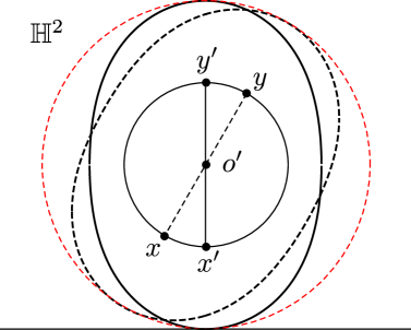
Figure 4. The Cassinian oval $C(x^{\prime},y^{\prime};b^{\prime})$ is tangent to $\partial\mathbb{H}^{2}$ while $C(x,y;b^{\prime})\subsetneq\mathbb{H}^{2}$.

Figure 5. The Cassinian oval $C(x,y;b)$ is tangent to $\partial\mathbb{H}^{2}$ while $C(x^{\prime\prime},y^{\prime\prime};b)\subsetneq\mathbb{H}^{2}$.

Theorem 3.16.

Let $x,y\in\mathbb{H}^{2}$ and $d=d(\frac{x+y}{2},\partial\mathbb{\mathbb{H}}^{2})$. Then

(3.19) $$\tilde{\tau}_{{\mathbb{H}}^{2}}(x,y)\geq\left\{\begin{array}[]{ll}\log\left(1+\sqrt{\frac{|x-y|}{d}}\right),&|x-y|>2\,d\,,\\ \log\left(1+\frac{2\,|x-y|}{\sqrt{4\,d^{2}+|x-y|^{2}}}\right),&|x-y|\leq 2\,d,\end{array}\right.$$

and

(3.20) $$\tilde{\tau}_{\mathbb{H}^{2}}(x,y)\leq\log\left(1+\frac{2|x-y|}{\sqrt{4\,d^{2}-|x-y|^{2}}}\right)\,,\quad|x-y|<2d\,.$$

Proof.

To prove inequalities (3.19), let $x^{\prime\prime}\,,y^{\prime\prime}$ be the same as in Lemma 3.15. The results follow from Lemma 3.15 and Lemma 3.13 immediately.

To prove inequality (3.20), let $x^{\prime}\,,y^{\prime}$ be the same as in Lemma 3.15. Since $d(x^{\prime},\partial\mathbb{H}^{2})=d-\frac{|x-y|}{2}$ and $d(y^{\prime},\partial\mathbb{H}^{2})=d+\frac{|x-y|}{2}$, together with Lemma 3.15 and Lemma 3.14, we have

$$\tilde{\tau}_{\mathbb{H}^{2}}(x,y)\leq\tilde{\tau}_{\mathbb{H}^{2}}(x^{\prime},y^{\prime}) =\log\left(1+\frac{|x-y|}{\sqrt{d(x^{\prime},\partial\mathbb{H}^{2})\,d(y^{\prime},\partial\mathbb{H}^{2})}}\right)$$

$$=\log\left(1+\frac{2|x-y|}{\sqrt{4\,d^{2}-|x-y|^{2}}}\right).$$

The proof is complete. ∎

4. The $\tilde{\tau}$-metric and the hyperbolic metric

In [13], Ibragimov showed the relation between the scale invariant Cassinian metric and the hyperbolic metric in the unit ball, while a statement about the sharpness of comparison was missing. In this section, we will provide the missing sharpness statement and study the same property in the upper half space.

Theorem 4.1.

For all $x,y\in\mathbb{B}^{n}$, we have

(4.2) $$\frac{1}{4}\rho_{\mathbb{B}^{n}}(x,y)\leq\tilde{\tau}_{\mathbb{B}^{n}}(x,y)\leq\rho_{\mathbb{B}^{n}}(x,y),$$

and both the inequalities are sharp. In addition, for all $x,y\in\mathbb{B}^{n}$, we have

(4.3) $$\tilde{\tau}_{\mathbb{B}^{n}}(x,y)\leq\frac{1}{2}\rho_{\mathbb{B}^{n}}(x,y)+\log\frac{5}{4},$$

and the inequality is sharp.

Proof.

For the inequalities see [13, Theorem 3.8].

For the sharpness of the left-hand side of inequalities (4.2), let $x=-y=te_{1}$ with $t\in(0,1)$. By Lemma 3.3(2) and (2.4), we have

$$\lim_{t\rightarrow 1^{-}}\frac{\tilde{\tau}_{\mathbb{B}^{n}}(x,y)}{\rho_{\mathbb{B}^{n}}(x,y)}=\lim_{t\rightarrow 1^{-}}\frac{\log\left(1+\frac{2t}{\sqrt{1-t^{2}}}\right)}{2\log\left(1+\frac{2t}{1-t}\right)}=\frac{1}{2}\lim_{t\rightarrow 1^{-}}\frac{\log\left(\frac{2t}{\sqrt{1-t^{2}}}\right)}{\log\left(\frac{2t}{1-t}\right)}=\frac{1}{4}\,.$$

For the sharpness of the right-hand side of inequalities (4.2), let $x=te_{1}$ and $y=(t+(1-t)^{2})e_{1}$ with $t\in(0,1)$. By Lemma 3.3(1) and (2.4), we have

$$\lim_{t\rightarrow 1^{-}}\frac{\tilde{\tau}_{\mathbb{B}^{n}}(x,y)}{\rho_{\mathbb{B}^{n}}(x,y)}=\lim_{t\rightarrow 1^{-}}\frac{\log\left(1+\frac{1-t}{\sqrt{t}}\right)}{\log\left(1+\frac{2(1-t)}{t(1+t)}\right)}=\lim_{t\rightarrow 1^{-}}\frac{\sqrt{t}(1+t)}{2}=1\,.$$

For the sharpness of inequality (4.3), let $x=(t+(1-t)^{2})e_{1}$ and $y=(t+(1-t)^{5})e_{1}$. By Lemma 3.3(1) and (2.4), we have

$$\lim_{t\rightarrow 0}\tilde{\tau}_{\mathbb{B}^{n}}(x,y)=\lim_{t\rightarrow 0}\log\left(1+\frac{(1-t)(3-3t+t^{2})}{\sqrt{4-6t+4t^{2}-t^{3}}}\right)=\log\frac{5}{2}$$

and

$$\lim_{t\rightarrow 0}\rho_{\mathbb{B}^{n}}(x,y)=\lim_{t\rightarrow 0}\log\left(\frac{1+t+(1-t)^{2}}{1+t+(1-t)^{5}}(4-6t+4t^{2}-t^{3})\right)=\log 4\,.$$

Hence

$$\lim_{t\rightarrow 0}\left(\tilde{\tau}_{\mathbb{B}^{n}}(x,y)-\frac{1}{2}\rho_{\mathbb{B}^{n}}(x,y)\right)=\log\frac{5}{4}\,.$$

This completes the proof. ∎

The following theorem shows the analogue of Theorem 4.1 in the upper half space.

Theorem 4.4.

For all $x,y\in\mathbb{H}^{n}$, we have

(4.5) $$\frac{1}{4}\rho_{\mathbb{H}^{n}}(x,y)\leq\tilde{\tau}_{\mathbb{H}^{n}}(x,y)\leq\rho_{\mathbb{H}^{n}}(x,y)\,,$$

and both the inequalities are sharp. In addition, for all $x,y\in\mathbb{H}^{n}$, we have

(4.6) $$\tilde{\tau}_{\mathbb{H}^{n}}(x,y)\leq\frac{1}{2}\rho_{\mathbb{H}^{n}}(x,y)+\log\frac{5}{4}\,,$$

and the inequality is sharp.

Proof.

Inequalities (4.5) are a consequence of Lemma 2.9 and Lemma 2.15.

For the sharpness of the left-hand side of inequalities (4.5), let $x=te_{1}+e_{n}$ and $y=e_{n}$ with $t>2$. By Lemma 3.13(1) and (2.3), we get

$$\lim_{t\rightarrow\infty}\frac{\tilde{\tau}_{\mathbb{H}^{n}}(x,y)}{\rho_{\mathbb{H}^{n}}(x,y)}=\lim_{t\rightarrow\infty}\frac{\log\left(1+\sqrt{t}\right)}{\log\left(1+\frac{t^{2}+\sqrt{t^{4}+4t^{2}}}{2}\right)}=\frac{1}{4}\,.$$

For the sharpness of the right-hand side of inequalities (4.5), let $x=te_{n}$ and $y=\frac{1}{t}e_{n}$ with $t>1$. By Lemma 3.14 and (2.5), we get

$$\lim_{t\rightarrow 1^{+}}\frac{\tilde{\tau}_{\mathbb{H}^{n}}(x,y)}{\rho_{\mathbb{H}^{n}}(x,y)}=\lim_{t\rightarrow 1^{+}}\frac{\log(1+(t-\frac{1}{t}))}{\log(1+(t^{2}-1))}=1\,.$$

To prove inequality (4.6), we first observe that

$$\inf_{\xi\in\mathbb{H}^{n}}|x-\xi||y-\xi|\geq x_{n}y_{n}\,,\quad{\rm for\,\,all}\,\,x,y\in\mathbb{H}^{n}\,,$$

and the equality holds when $y-x$ is orthogonal to $\partial\mathbb{H}^{n}.$

Since

$$1+\sqrt{2({\rm ch}\,t-1)}=1+e^{t/2}-e^{-t/2}\leq\frac{5}{4}e^{t/2}\,,\quad{\rm for\,\,all}\,\,t\geq 0\,,$$

together with (2.3), we have

$$\tilde{\tau}_{\mathbb{H}^{n}}(x,y) \leq\log\left(1+\frac{|x-y|}{\sqrt{x_{n}\,y_{n}}}\right)$$

$$=\log\left(1+\sqrt{2({\rm ch}\,\rho_{\mathbb{H}^{n}}(x,y)-1)}\right)$$

$$\leq\frac{1}{2}\,\rho_{\mathbb{H}^{n}}(x,y)+\log\frac{5}{4}\,.$$

To prove the sharpness of inequality (4.6), let $x=2e_{n}$ and $y=\frac{1}{2}e_{n}$. By Lemma 3.14 and (2.5), we get

$$\tilde{\tau}_{\mathbb{H}^{n}}(x,y)=\log\frac{5}{2}\quad{\rm and}\quad\rho_{\mathbb{H}^{n}}(x,y)=\log 4\,.$$

Hence

$$\tilde{\tau}_{\mathbb{H}^{n}}(x,y)=\frac{1}{2}\rho_{\mathbb{H}^{n}}(x,y)+\log\frac{5}{4}.$$

This completes the proof. ∎

5. The $\tilde{\tau}$-metric and Möbius transformations

Ibragimov studied the distortion properties of $\tilde{\tau}$-metric under Möbius transformations of the unit ball [13, Theorem 4.1, Theorem 4.2]. Later, Mohapatra and Sahoo considered the same problem in the punctured unit ball [18, Theorem 2.1]. For instance, the following quasi-isometry property was obtained in [13].

Theorem 5.1.

[13, Theorem 4.2] If $f:\overline{{\mathbb{R}}}^{n}\to\overline{{\mathbb{R}}}^{n}$ is a Möbius transformation with $f\mathbb{B}^{n}=\mathbb{B}^{n}$, then for all $x,y\in\mathbb{B}^{n}$, we have

(5.2) $$\frac{1}{2}\tilde{\tau}_{\mathbb{B}^{n}}(x,y)-\log\frac{5}{4}\leq\tilde{\tau}_{\mathbb{B}^{n}}(f(x),f(y))\leq 2\tilde{\tau}_{\mathbb{B}^{n}}(x,y)+\log\frac{5}{4}\,.$$

In this section, we continue the investigation on the distortion of $\tilde{\tau}$-metric of general domains under Möbius transformations. In particular, we show that in (5.2) the additional constant $\log\frac{5}{4}$ can be removed and the constants $\frac{1}{2}$ and $2$ are the best possible.

Theorem 5.3.

If $D$ and $D^{\prime}$ are proper subdomains of $\mathbb{R}^{n}$ and if $f:\overline{{\mathbb{R}}}^{n}\to\overline{{\mathbb{R}}}^{n}$ is a Möbius transformation with $fD=D^{\prime}$, then for all $x,y\in D$, we have

$$\frac{1}{2}\tilde{\tau}_{D}(x,y)\leq\tilde{\tau}_{D^{\prime}}(f(x),f(y))\leq 2\tilde{\tau}_{D}(x,y)\,.$$

Proof.

The proof follows from Lemma 2.18 and Lemma 2.17 immediately. ∎

The following theorem shows that the above constants $\frac{1}{2}$ and $2$ can not be improved.

Theorem 5.4.

Let $f:{\mathbb{H}}^{n}\to{\mathbb{B}}^{n}=f{\mathbb{H}}^{n}$ be a Möbius transformation. Then for all $x,y\in\mathbb{H}^{n}$ , we have

$$\frac{1}{2}\tilde{\tau}_{\mathbb{H}^{n}}(x,y)\leq\tilde{\tau}_{\mathbb{B}^{n}}(f(x),f(y))\leq 2\tilde{\tau}_{\mathbb{H}^{n}}(x,y),$$

and the constants $\frac{1}{2}$ and $2$ are the best possible.

Proof.

The inequalities are clear from Theorem 5.3. Next we show the sharpness of the inequalities.

Since $\tilde{\tau}$-metric is invariant under translations and stretchings of $\mathbb{H}^{n}$ onto itself and orthogonal transformations of $\mathbb{B}^{n}$ onto itself, it suffices to consider

$$f(z)=-e_{n}+\frac{2(z+e_{n})}{|z+e_{n}|^{2}}\,.$$

Let $x=te_{n}$ and $y=\frac{1}{t}e_{n}$ with $t>1\,.$ Then

$$f(x)=-\frac{t-1}{t+1}e_{n}\quad\quad\quad~{}~{}~{}{\rm and}\quad\quad\quad~{}~{}~{}f(y)=\frac{t-1}{t+1}e_{n}\,.$$

By Lemma 3.3(2) and Lemma 3.14, we get

$$\lim_{t\rightarrow\infty}\frac{\tilde{\tau}_{\mathbb{B}^{n}}\left(f(x),f(y)\right)}{\tilde{\tau}_{\mathbb{H}^{n}}(x,y)}=\lim_{t\rightarrow\infty}\frac{\log\left(1+(\sqrt{t}-\frac{1}{\sqrt{t}})\right)}{\log\left(1+(t-\frac{1}{t})\right)}=\lim_{t\rightarrow\infty}\frac{\log\left(\sqrt{t}-\frac{1}{\sqrt{t}}\right)}{\log\left(t-\frac{1}{t}\right)}=\frac{1}{2}\,.$$

Let $x=te_{1}+e_{n}$ and $y=e_{n}$ with $t>2$. Then

$$f(x)=\frac{2t}{t^{2}+4}e_{1}-\frac{t^{2}}{t^{2}+4}e_{n}\quad\quad\quad~{}~{}~{}{\rm and}\quad\quad\quad~{}~{}~{}f(y)=0\,.$$

By Remark 3.4 and Lemma 3.13(1), we get

$$\lim_{t\rightarrow\infty}\frac{\tilde{\tau}_{\mathbb{B}^{n}}\left(f(x),f(y)\right)}{\tilde{\tau}_{\mathbb{H}^{n}}(x,y)}=\lim_{t\rightarrow\infty}\frac{\log\left(1+\frac{t}{\sqrt{t^{2}+4-t\sqrt{t^{2}+4}}}\right)}{\log\left(1+\sqrt{t}\right)}\\ =\lim_{t\rightarrow\infty}\frac{\log\left(\frac{t}{\sqrt{t^{2}+4-t\sqrt{t^{2}+4}}}\right)}{\log{\sqrt{t}}}=2\,.$$

This completes the proof. ∎

Acknowledgments

This research was supported by National Natural Science Foundation of China (NNSFC) under Grant No.11771400 and No.11601485 , and Science Foundation of Zhejiang Sci-Tech University (ZSTU) under Grant No.16062023 -Y.

References

- [1] G. D. Anderson, M. K. Vamanamurthy, and M. Vuorinen, Conformal invariants, inequalities, and quasiconformal maps. J. Wiley, 1997.
- [2] A. F. Beardon, The geometry of discrete groups. Graduate Texts in Math., Vol. 91, Springer-Verlag, New York, 1983.
- [3] A. F. Beardon, The Apollonian metric of a domain in . Quasiconformal mappings and analysis (Ann Arbor, MI, 1995), 91–108, Springer, New York, 1998.
- [4] O. Dovgoshey, P. Hariri, and M. Vuorinen, Comparison theorems for hyperbolic type metrics. Complex Var. Elliptic Equ. 61 (2016), 1464–1480.
- [5] M. Fujimura, M. Mocanu, and M. Vuorinen, Barrlund’s distance function and quasiconformal maps. Complex Var. Elliptic Equ. 2020 (to appear).
- [6] F. W. Gehring and K. Hag, The ubiquitous quasidisk. With contributions by Ole Jacob Broch. Mathematical Surveys and Monographs, 184. American Mathematical Society, Providence, RI, 2012. xii+171 pp.
- [7] F. W. Gehring and B. P. Palka, Quasiconformally homogeneous domains. J. Analyse Math. 30 (1976), 172–199.
- [8] P. Hariri, R. Klén, M. Vuorinen, and X. Zhang, Some remarks on the Cassinian metric. Publ. Math. Debrecen 90 (2017), 269–285.
- [9] P. Hästö, A new weighted metric: the relative metric I. J. Math. Anal. Appl. 274 (2002), 38–58.
- [10] P. Hästö, A new weighted metric: the relative metric. II. J. Math. Anal. Appl. 301 (2005), 336–353.
- [11] P. Hästö, Inequalities of generalized hyperbolic metrics. Rocky Mountain J. Math. 37 (2007), 189–202.
- [12] Z. Ibragimov, The Cassinian metric of a domain in . Uzbek. Math. Zh. (2009), 53–67.
- [13] Z. Ibragimov, A scale-invariant Cassinian metric. J. Anal. 24 (2016), 111–129.
- [14] Z. Ibragimov, M. R. Mohapatra, S. K. Sahoo, and X. Zhang, Geometry of the Cassinian metric and its inner metric. Bull. Malays. Math. Sci. Soc. 40 (2017), 361–372.
- [15] Z. Ibragimov, Möbius invariant Cassinian metric. Bull. Malays. Math. Sci. Soc. 42 (2019), 1349–1367.
- [16] R. Klén, H. Lindén, M. Vuorinen, and G. Wang, The visual angle metric and Möbius transformations. Comput. Methods Funct. Theory 14 (2014), 577–608.
- [17] R. Klén, M. R. Mohapatra, and S. K. Sahoo, Geometric properties of the Cassinian metric. Math. Nachr. 290 (2017), 1531–1543.
- [18] M. R. Mohapatra and S. K. Sahoo, Mapping properties of a scale invariant Cassinian metric and a Gromov hyperbolic metric. Bull. Aust. Math. Soc. 97 (2018), 141–152.
- [19] M. R. Mohapatra and S. K. Sahoo, A Gromov hyperbolic metric vs the hyperbolic and other related metrics. Comput. Methods Funct. Theory 18 (2018), 473–493.
- [20] P. Seittenranta, Möbius-invariant metrics. Math. Proc. Cambridge Philos. Soc. 125 (1999), 511–533.
- [21] M. Vuorinen, Conformal geometry and quasiregular mappings. Lecture Notes in Math. 1319, Springer-Verlag, Berlin, 1988.
- [22] G. Wang and M. Vuorinen, The visual angle metric and quasiregular maps. Proc. Amer. Math. Soc. 144 (2016), 4899–4912.
- [23] X. Zhang, Comparison between a Gromov hyperbolic metric and the hyperbolic metric. Comput. Methods Funct. Theory 18 (2018), 717–722.