The Type II-P Supernova 2017eaw: from explosion to the nebular phase

Abstract

The nearby SN 2017eaw is a Type II-P (“plateau”) supernova showing early-time, moderate CSM interaction. We present a comprehensive study of this SN including the analysis of high-quality optical photometry and spectroscopy covering the very early epochs up to the nebular phase, as well as near-UV and near-infrared spectra, and early-time X-ray and radio data. The combined data of SNe 2017eaw and 2004et allow us to get an improved distance to the host galaxy, NGC 6946, as $D\sim 6.85$ $\pm 0.63$ Mpc; this fits in recent independent results on the distance of the host and disfavors the previously derived (30 % shorter) distances based on SN 2004et. From modeling the nebular spectra and the quasi-bolometric light curve, we estimate the progenitor mass and some basic physical parameters for the explosion and the ejecta. Our results agree well with previous reports on a RSG progenitor star with a mass of $\sim 15-16$ M_⊙. Our estimation on the pre-explosion mass-loss rate ($\dot{M}\sim 3\times 10^{-7}-$ $1\times 10^{-6}M_{\odot}$ yr^-1) agrees well with previous results based on the opacity of the dust shell enshrouding the progenitor, but it is orders of magnitude lower than previous estimates based on general light-curve modeling of Type II-P SNe. Combining late-time optical and mid-infrared data, a clear excess at 4.5 $\mu$m can be seen, supporting the previous statements on the (moderate) dust formation in the vicinity of SN 2017eaw.

1 Introduction

Recently, the growing number of well-observed (i.e. having high signal-to-noise, high cadence data spanning a wide wavelength range) Type II supernovae (SNe) revealed important new details about their progenitors, explosion mechanisms and diversity (see e.g. Valenti et al., 2016, and references therein). For example, photometry and spectroscopy taken at the earliest phases, during and after shock breakout, turned out to be especially useful for constraining the progenitor radii and/or probing the nearby circumstellar matter (Garnavich et al., 2016; Khazov et al., 2016).

SN 2017eaw was discovered by P. Wiggins on UT 2017 May 14.238 at a brightness of 12.8 mag (Wiggins, 2017). Within a few hours the presence of the new transient was confirmed by Dong & Stanek (2017) based on images taken by the Las Cumbres Observatory (LCO) 1m telescope at McDonald Observatory, Texas. The object was classified first as a young Type II SN (Cheng et al., 2017; Tomasella et al., 2017), while, soon after, Xiang et al. (2017) found that early spectra of SN 2017eaw matches well with that of young Type II-P explosions; later, the classification has been confirmed by photometry.

SN 2017eaw appeared in NGC 6946, at 61.0^′′ west and 143.0^′′ north from the center of the galaxy. The host is a nearby, face-on spiral galaxy, which has produced around a dozen known SNe and other luminous transients including the Type II-L SN 1980K, Type II-P SNe 1948B, 2002hh and 2004et, and the SN impostor 2008S. The first precise astrometric position of SN 2017eaw, based on ground-based imaging, has been given by Sárneczky et al. (2017): $\alpha$ = 20^h34^m44^s.238, $\delta$ = $+$60^d11^′36$\arcsec$.00 (with RMS uncertainties of $\Delta\alpha$ = 0.08″and $\Delta\delta$ = 0.09″). Later, Kilpatrick & Foley (2018) determined a very similar, even more precise position of the object on post-explosion Hubble Space Telescope (HST) images: $\alpha$ = 20^h34^m44^s.272, $\delta$ = $+$60^d11^′36$\arcsec$.008 (with an uncertainty of $\sim$0.002-0.003″in both $\alpha$ and $\delta$).

Since SN 2017eaw is one of the closest CC SNe to date and it appeared in a host galaxy that is being monitored almost continuously, the search for the potential progenitor in archival imaging data was started right after the announcement of discovery. The first hints of a possible progenitor were reported by Khan (2017, based on mid-infrared Spitzer Space Telescope images), Drake et al. (2017, based on optical Catalina Sky Survey images), and van Dyk et al. (2017, using HST ACS/WFC F814W images); all of these findings suggested the presence of a red supergiant (RSG) star at the position of the SN. The detailed analysis by Kilpatrick & Foley (2018), based on archival HST and Spitzer images, confirmed the RSG progenitor ($log(L/L_{\odot}$) = 4.9, $T_{\text{eff}}$ = 3350K, M${}_{\text{ini}}$ = 13 M_⊙) obscured by a dust shell; these results agree well with that of Rui et al. (2019) based on a similar analysis. In the frameworks of comprehensive studies, two other groups also published their findings on the progenitor candidate of SN 2017eaw. Williams et al. (2018) carried out an age-dating study of the surrounding stellar populations of nearby (historic) CC SNe on new HST images; based on that they derived a somewhat smaller mass for the assumed progenitor of SN 2017eaw ($\sim$9 M_⊙). Johnson et al. (2018) presented the results of a long-term multi-channel optical monitoring of the progenitors of Type II SNe; they found a general brightness variability smaller than 5-10$\%$, which is in agreement with the known properties of RSG stars.

SN 2017eaw has been the target of several multi-wavelength observing campaigns since its early phase; however, only a few datasets have been published to date. Tsvetkov et al. (2018) presented the results of their BVRI photometric campaign covering the first $\sim$200 days. Rho et al. (2018) obtained and analyzed near-infrared (near-IR) spectra spanning the time interval 22$-$205 days after discovery, while Kilpatrick & Foley (2018) published only a single optical spectrum taken during the photospheric phase. Radio and X-ray (non)detections have been also reported (see Section 4.2).

In this paper we present a comprehensive study on the early- and late-time properties of SN 2017eaw. First, we present our ground-based spectroscopic and photometric observations in Section 2. After that we give the details on the comparison of the light curves and spectra with those of other SNe II-P, the extraction of physical parameters from bolometric light curve modeling, and the estimation of the distance of the host galaxy based on the combined data of SNe 2017eaw and 2004et. We also present our findings from the analysis of early-time radio and X-ray (non)detections and of late-time mid-infrared data of SN 2017eaw, and interpret these as potential signs of circumstellar interaction and dust formation in the vicinity of the explosion site, respectively. In Section 4, we discuss our results and, finally, in Section 5, we present our conclusions.

2 Observations

This section contains the description of the observational data on SN 2017eaw collected with various ground- and space-based instruments. All data will be publicly released via WIseREP

2.1 Photometry

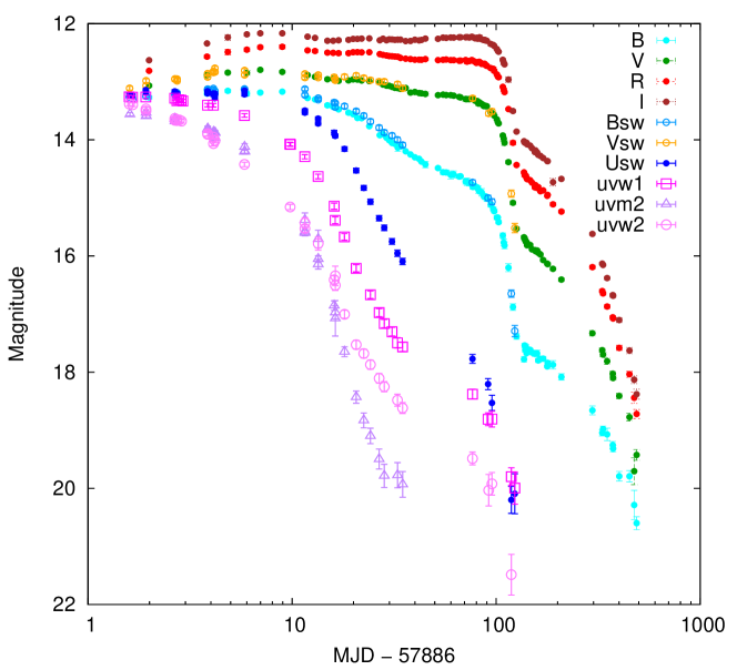
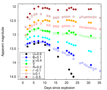
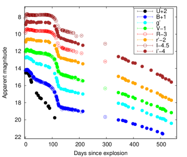
Figure 1: Top panel: Multi-colour light curves of SN 2017eaw from Konkoly and Swift/UVOT. The Swift UV data have been shifted by +1 magnitude for better visibility. Bottom panel: The Konkoly BVRI (open circles) and LCO UBV$g^{\prime}r^{\prime}i^{\prime}$ (filled circles) photometric data during the first month (bottom left) and up to +545 days (bottom right panel).

Ground-based photometric observations for SN 2017eaw were obtained from the Piszkéstető Mountain Station of Konkoly Observatory, Hungary. We used the 0.6/0.9 m Schmidt-telescope with the attached liquid-cooled FLI Proline PL16801 4096 $\times$ 4096 CCD (FoV 70 $\times$ 70 arcmin²) equipped with Bessell BVRI filters. The CCD frames were bias-, dark- and flatfield-corrected by applying standard IRAF routines. To obtain the Konkoly BVRI magnitudes, we carried out PSF photometry on the SN and 5 local comparison (tertiary standard) stars using the allstar task in IRAF. We applied an aperture radius of 6″and a background annulus from 7″to 10″for SN 2017eaw as well as for the local comparison stars. The magnitudes of the local comparison stars were determined from their PS1-photometry after transforming the PS1 gri magnitudes to the Johnson-Cousins BVRI system.

Long-term photometric data were collected as part of the Global Supernova Project by the Las Cumbres Observatory (LCO). Using lcogtsnpipe (Valenti et al., 2016), a PyRAF-based photometric reduction pipeline, we measured PSF photometry of the SN. Because the SN is well-separated from its host galaxy, image subtraction is not required. Local sequence stars were calibrated to $g^{\prime}r^{\prime}i^{\prime}$ AB magnitudes from the APASS catalog (Henden et al., 2016) and to standard fields (e.g. L113) observed on the same night at the same observatory site using UBV magnitudes from Landolt (1992).

The ground-based optical observations were supplemented by the available Neil Gehrels Swift Observatory (hereafter Swift, Gehrels et al., 2004; Burrows et al., 2005) data taken with the Ultraviolet-Optical Telescope (UVOT) (Roming et al., 2005) and reduced using standard HEAsoft tasks. Individual frames were summed with the uvotimsum task. Magnitudes were determined via aperture photometry using the task uvotsource and adopting the most recent zero points (Breeveld et al., 2011).

The results of our LCO UBV$g^{\prime}r^{\prime}i^{\prime}$ (in Vega-magnitudes for UBV and AB-magnitudes for $g^{\prime}r^{\prime}i^{\prime}$ bands), Konkoly BVRI, and Swift photometry (both in Vega-magnitudes) are shown in Fig. 1; the data are also presented in Tables A1, A2, and A3, respectively. Intrinsic photometric errors are typically below 0.05 mag, while the overlapping photometric datasets – LCO/Konkoly/Swift BV magnitudes, as well as our BVRI data and that of Tsvetkov et al. (2018) – are generally consistent within $\sim$0.1 mag.

2.2 Spectroscopy

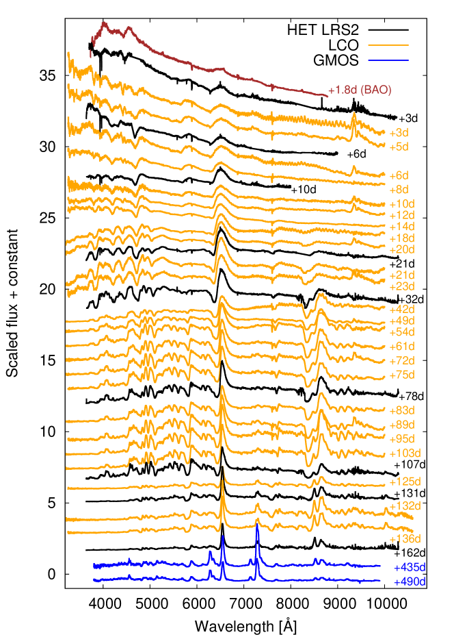
Figure 2: Optical spectra of SN 2017eaw obtained with HET LRS2 (black) and Gemini-North GMOS-N (blue), and from LCO sites (orange). An additional public spectrum obtained at May 14 from the Beijing Astronomical Observatory (BAO) is also shown (brown).

A number of low-resolution optical spectra (R$\sim$400$-$700, in the 370$-$1050 nm range) were collected at LCO sites using the FLOYDS instruments. Additionally, a sequence of optical spectra on SN 2017eaw was taken with the Low Resolution Spectrograph 2 (LRS2) mounted on the 10m Hobby-Eberly Telescope. LRS2 consists of two dual-arm spectrographs covering the 370$-$470 and 460$-$700 nm region (LRS2-B UV- and Orange arm) and the 650$-$842 and 818$-$1050 nm region (LRS2-R Red- and IR-arm), respectively, with an average spectral resolution of about 1500 (Chonis et al., 2016). Both arms are fiber-fed by their own Integral Field Unit (IFU) having 280 fibers packed densely to fully cover a $12\times 6$ arcsec² field of view. For further details on the instrument and the data reduction see e.g. Li et al. (2018).

Swift took two near-ultraviolet (near-UV) spectra with UVOT/UGRISM covering the 200$-$500 nm regime. These data were downloaded from the Swift Data Archive and extracted using the HEAsoft task uvotimgrism.

Furthermore, five near-IR spectra were taken with the 3.0-m NASA Infrared Telescope Facility (IRTF) and the SpeX spectrograph (Rayner et al., 2003). The data were taken in “SXD” mode, with wavelength coverage from $\sim$0.8-2.4 $\mu$m, cross-dispersed into six orders. The observations were taken using the classic ABBA technique for improved sky-subtraction, and an A0V star was observed for telluric correction. For further details of the observational setup and execution, see Hsiao et al. (2019). The data were reduced using the publicly available Spextool software package (Cushing et al., 2004), and the telluric corrections were performed with the XTELLCOR software suite (Vacca et al., 2003).

Optical spectra were obtained during the nebular phase on day 220, 435, and 491. The first spectrum was taken on 2017-12-19.23 UT with the Low Resolution Imaging Spectrometer (LRIS) (Oke et al., 1995; McCarthy et al., 1998; Rockosi et al., 2010) at the 10m W. M. Keck Observatory (2017B, project code U109, PI: Valenti). The spectrum was taken using a 1″aperture with the 560 dichroic to split the beam between the 600/4000 grism on the blue side and the 400/8500 grating on the red side. Taken together, the merged spectrum spans $\sim$3200$-$10,200Å. Data were reduced in a standard way using the LPIPE pipeline . The remaining spectra were observed on 2018-07-22.52 UT and 2018-09-16.31 UT with the Gemini Multi-Object Spectrograph (GMOS) (Hook et al., 2004; Gimeno et al., 2016) mounted on the 8m Frederick C. Gillett Gemini North telescope (program ID: GN-2018B-Q-204, PI: Bostroem). Observations were taken using a 1″aperture utilizing a red setup and a blue setup to obtain wavelength coverage from 3450$-$9900Å. The red setup observations were taken with the R400 grating and the OG515 blocking filter with a resolution of R$\sim$1918. The blue setup observations were taken with the B600 grating with a resolution of R$\sim$1688. The spectra were reduced using a combination of the Gemini iraf package and custom Python scripts . Extracted spectra were scaled to photometry interpolated or extrapolated to the date of observation.

The journal of all spectroscopic observations is given in Table A4. The sequence of optical spectra is plotted in Fig 4, while the detailed analysis of all optical, near-UV and near-IR spectra are presented in Section 3.

3 Analysis and results

Table 1: Basic data of Type II-P SNe used for comparison

Name	Host galaxy	Date of explosion	$z$	$D$ (Mpc)	$E(B-V)_{\text{tot}}$	Source
		(JD$-$2,400,000)			(mag)
SN 2017eaw	NGC 6946	57886.5 $\pm$ 1.0	0.00013	6.85 $\pm$ 0.63	0.41	1, 2
SN 2004et	NGC 6946	53270.5 $\pm$ 1.0	0.00013	6.85 $\pm$ 0.63	0.41	1, 2
SN 2012aw	NGC 3351	56002.6	0.00260	9.9 $\pm$ 0.1	0.07	3
SN 2013fs	NGC 7610	56571.1	0.01190	51.0 $\pm$ 3.0	0.05	4
SN 2016X	UGC 08041	57405.9	0.00441	15.2 $\pm$ 2.0	0.04	5
SN 2016bkv	NGC 3184	57467.5	0.00198	14.4 $\pm$ 0.3	0.01	6, 7

Notes. Parameters marked with boldface have been determined in this work. References: 1) This work; 2) Maguire et al. (2010b); 3) Bose et al. (2013); 4) Yaron et al. (2017); 5) Huang et al. (2018); 6) Hosseinzadeh et al. (2018); 7) Nakaoka et al. (2018). Redshifts are adopted from NASA/IPAC Extragalactic Database (NED, https://ned.ipac.caltech.edu).

First, we estimate some basic parameters of SN 2017eaw: the moment of explosion ($t_{0}$), the interstellar extinction toward the SN, and the distance to the host galaxy.

We adopt $t_{0}$ = 2,457,886.5$\pm 1.0$ JD (May 13.0$\pm$1.0 UT) as the moment of explosion of SN 2017eaw. This value is strengthened by our distance estimation analysis (see Section 3.3), and suits well to both the date of discovery (May 14.2, 2017) and the epoch of last non-detection (May 12.2, 2017).

Finding the true value of the total extinction in the line-of-sight of SN 2017eaw does not seem to be trivial. Using the reddening map of Schlafly & Finkbeiner (2011), we get $E(B-V)_{\text{gal}}$=0.30 mag for the Galactic extinction. For the total extinction, several estimates based on empirical relations between the total reddening and equivalent widths (EWs) of Na I D lines exist in the literature: for example, Tomasella et al. (2017) derived $E(B-V)_{\text{tot}}$=0.22 mag for the total (Galactic+host) extinction using the formulae by Turatto et al. (2003), which is lower than the Galactic component given above, while Kilpatrick & Foley (2018) determined $E(B-V)_{\text{tot}}$=0.34 mag following the method by Poznanski et al. (2012).

The $\sim 0.1$ mag difference between these two estimates illustrate the issue that these empirical relations may suffer from relatively high systematic errors (see e.g. Blondin et al., 2009; Poznanski et al., 2011; Faran et al., 2014). This belief is confirmed by our own analysis. Based on our HET spectra, we also determined the EWs of Na I D1 and D2 features as well as that of the combined line profile (D1+D2) as 0.8, 1.1, and 1.7Å, respectively. Because of the very low redshift of SN 2017eaw, the Na I D doublet at 5890$-$5895Å originating from the Milky Way may be blended with the same features formed in the interstellar medium (ISM) of the host galaxy (and maybe in the CSM around the SN site). In any case, such high EW values would imply $E(B-V)>1$ mag according to the empirical relations given by Poznanski et al. (2012). Since the EW(Na I)$-E(B-V)$ relation is suspected to saturate at $E(B-V)\gtrsim 0.2$ mag, these measurements probably overestimate the total reddening toward SN 2017eaw.

Diffuse Interstellar Band (DIB) features offer an independent and sometimes more reliable way to estimate the interstellar reddening. In the same HET spectrum as above we measured the EW of the unresolved blend of Galactic and host DIB 5780Å feature and got $\sim 0.31$Å. Repeating the same measurement but using a public spectrum of SN 2004et, a Type II-P SN that occurred in the same host galaxy, resulted in EW(DIB) $\sim 0.19$Å (see Fig. 3). These values correspond to $E(B-V)$ $\sim$0.52 and $\sim$0.32 mag, respectively, following Phillips et al. (2013), who applied the method by Friedman et al. (2011).

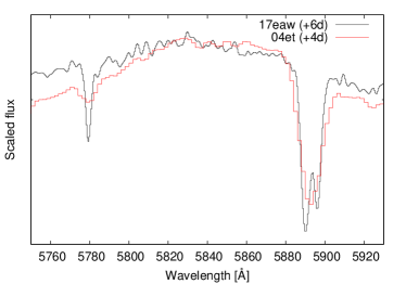
Figure 3: Region of DIB 5780Å and Na I D1 & D2 lines on both the +6d HET spectrum of SN 2017eaw and the +4d spectrum of SN 2004et (see the text regarding the estimation of total extinction in Section 3.)

For SN 2004et, Zwitter et al. (2004) determined $E(B-V)_{\text{tot}}$=0.41 mag based on the method of Munari & Zwitter (1997), which was also adopted by Maguire et al. (2010b). Since the optical spectra of SNe 2017eaw and 2004et appear to be very similar (see Section 3.2), including Na D profiles, and this $E(B-V)$ value is close to the mean of the results from the various estimates detailed above, in the rest of this paper we adopt and use $E(B-V)_{\text{tot}}$=0.41 mag as the total reddening toward SN 2017eaw, but note that the uncertainty of this value is at least $\pm 0.1$ mag as explained above.

Similarly, we use $D$ = 6.85 $\pm$ 0.63 Mpc for the distance of the host galaxy that comes from our own detailed analysis using various methods and the combination of other recently published distances to NGC 6946 (see Section 3.3).

In the followings we present a detailed photometric and spectroscopic study of SN 2017eaw, comparing the results with those of several other Type II-P SNe (see Table 1). All the fluxes were dereddened using the Galactic reddening law parametrized by Fitzpatrick & Massa (2007) assuming $R_{\text{V}}$ = 3.1.

3.1 Photometric comparison

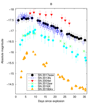
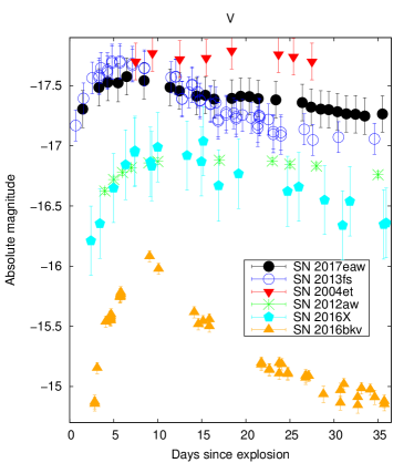
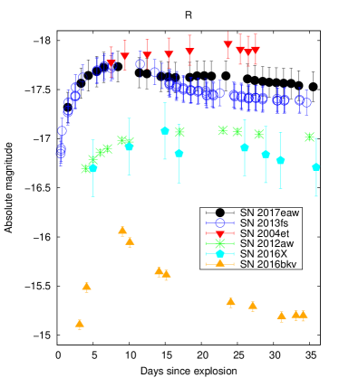
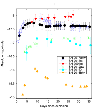
Figure 4: Early optical light curves of SN 2017eaw compared to those of other normal or interacting Type II-P SNe.

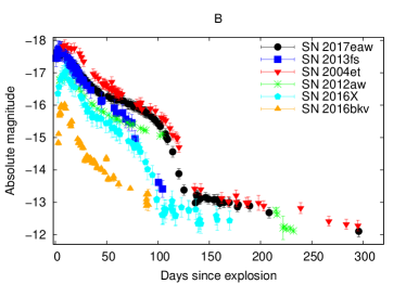
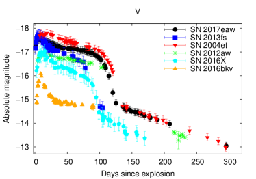
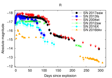
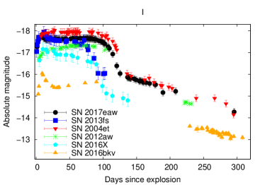
Figure 5: Full optical light curves of SN 2017eaw compared to those of other normal or interacting Type II-P SNe.

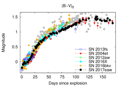
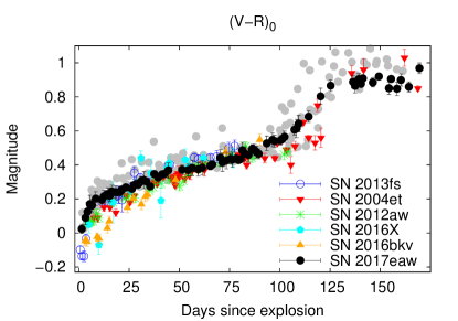
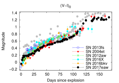
Figure 6: Dereddened colour curves of SN 2017eaw compared to those of other normal or interacting Type II-P SNe. Data marked with coloured symbols are adopted from sources given in Table 1, while all other data (grey circles) are from Faran et al. (2014).

We have selected several recent, well-observed Type II-P SNe for both photometric and spectroscopic comparison, including “normal” (but slightly superluminous) Type II-P SN 2004et (that appeared in the same host as SN 2017eaw), “normal” (but slightly subluminous) SN 2012aw, early-caught and strongly interacting SN 2013fs, early-caught and slightly subluminous SN 2016X, and early-time interacting, subluminous SN 2016bkv. Table 1 lists the basic data of the selected objects as well as their references.

Figs. 4 and 5 show the early-time and long-term absolute BVRI light curves (LCs) of SN 2017eaw together with that of the other selected SNe, respectively (absolute magnitudes were calculated using the distances and reddening values presented in Table 1). As can be seen in Fig. 4, SN 2017eaw shows a small, early bump peaking at $\sim$6-7 days after explosion in all optical channels. This behaviour resembles quite well that of SN 2013fs, and supposed to be the sign of early-time circumstellar interaction (Yaron et al., 2017; Morozova et al., 2017, 2018; Bullivant et al., 2018); this topic is further analyzed in Section 4.2.

After the early, small bump, SN 2017eaw shows a long plateau up to $\sim$100 days just as “normal” SNe II-P (e.g. 2004et), which probably indicates that the masses of the H-envelopes are similar in these cases (unlike SN 2013fs, whose plateau drops at $\sim$25 days earlier).

In Fig. 6 we present the reddening-corrected colour curves of a sample of SNe II-P. Basically, SN 2017eaw seems to follow the colour evolution of other II-P ones. The $(B-V)_{0}$ colour is quite blue in the early phases, but evolves relatively rapidly towards redder colours as the ejecta expands and cools; at $\sim$125 days, there is a transition peak after which the $(B-V)_{0}$ colour becomes gradually bluer. $(V-R)_{0}$ and $(V-I)_{0}$ evolve more slowly, and these curves become relatively flat after $\sim$125 days (in part because in this phase the SN II photometric evolution, which depends on the ⁵⁶Co decay, is approximately the same in all bands, see e.g. Galbany et al., 2016). Nevertheless, we note that, on one hand, the colour data are quite uncertain for most of the selected SNe after $\sim$100 days (sometimes there are no data at all), and, on the other hand, the reddening of several SNe – including 2017eaw and 2004et – are somewhat uncertain (as we described above).

3.2 Spectroscopic comparison

Based on our observational dataset on SN 2017eaw and published data on other Type II-P SNe listed in Table 1, we carried out a detailed comparative spectroscopic analysis. First, all observed spectra were corrected for the recession velocity of their host galaxies and for the total reddening/extinction listed in Table 1.

3.2.1 Optical spectra

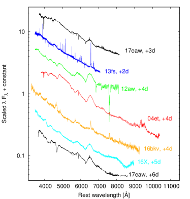
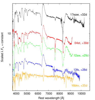
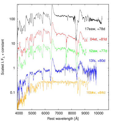
Figure 7: Optical spectra of SN 2017eaw compared to those of other normal or interacting Type II-P SNe. All spectra are corrected for redshift and extinction.

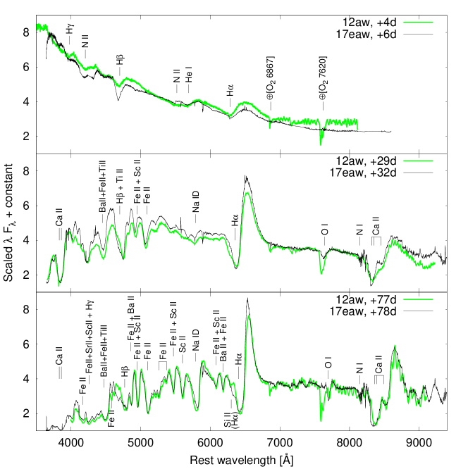
Figure 8: Line identification based on the SYNOW modeling of SN 2012aw (Bose et al., 2013). Note that at days +77/78, the small absorption component on the blue side of the H$\alpha$ P-Cygni profile may be a high velocity H feature instead of Si II 6355Å, see Gutiérrez et al. (2017).

In Fig. 7, we present the comparison of the optical spectra of SN 2017eaw with those of other SNe used above for the photometric comparison, selecting three ranges of epochs: 2-6 days, 28-35 days, and 78-84 days (upper left, upper right, and bottom panels, respectively; data sources are listed in Table 1). In general, the spectral evolution of SN 2017eaw follows the same trend that can be usually seen in Type II-P SNe; however, minor differences can also be found among the spectra.

The differences are most apparent during the early days. Both SNe 2013fs (Yaron et al., 2017; Bullivant et al., 2018) and 2016bkv (Hosseinzadeh et al., 2018; Nakaoka et al., 2018) have been found to exhibit a short-lived but intense circumstellar interaction: they showed numerous narrow emission lines during the first few days after explosion. At the same time, neither SN 2016X (Huang et al., 2018) nor SN 2017eaw showed any similar phenomenon, even though an early-time moderate CSM interaction may have taken place in 2017eaw (see also Section 4.2), similar to the “normal” Type II-P SNe 2004et and 2012aw (we note that, based on a very recent paper of Rui et al., 2019, a weak narrow H$\alpha$ line was observed in the 1.4d spectrum of SN 2017eaw). At $\sim$3 months, all spectra look very similar to each other except those of the low-luminosity SN 2016bkv, which shows much weaker H$\alpha$ and Ca II features and some further, incredibly narrow features compared to other objects. Note that while SNe 2017eaw, 2004et, and 2012aw are all in the plateau phase at this time, SN 2013fs is already in the declining phase, while in the case of SN 2016bkv, LC sampling is too poor to observe the transition (see Fig. 5).

The spectral similarity between SN 2017eaw, SN 2004et and 2012aw is even more pronounced when their spectrum models, computed with SYNOW, are compared. SN 2012aw is selected as a reference because SYNOW models for this SN are available (Bose et al., 2013). We adopted this model sequence for identifying the main features in the spectra of SN 2017eaw at three selected epochs (see Fig. 8). As can be seen, all the key spectral features appear with very similar line strengths in both spectra, except maybe H$\beta$ at the earliest epoch, and Si II 6355Å that seems to be somewhat stronger and at higher velocity in the +78d spectrum of SN 2017eaw than in SN 2012aw.

3.2.2 Velocity determination

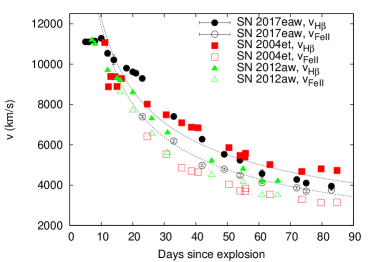
Figure 9: Left: velocity curves of SN 2017eaw compared to those of Type II-P SNe 2004et (Takáts & Vinkó, 2012) and 2012aw (Bose et al., 2013). Open and filled symbols denote velocities calculated from the Doppler-shift of the absorption minima of Fe II 5169Å  and H$\beta$ lines, respectively. Dotted and dashed lines show the fitted curves of $v_{\text{FeII}}$(t)/$v_{\text{FeII}}$(50)=(t/50)^{-0.567±0.021} and $v_{\text{H}\beta}$(t)/$v_{\text{H}\beta}$(50)=(t/50)^{-0.499±0.020}, respectively (see text for details). Right: The relation between the measured $v_{\text{FeII}}$ and $v_{\text{H}\beta}$ values.

Using our optical spectra, we also determined the H$\beta$ and Fe II 5169Å line velocities for SN 2017eaw ($v_{\text{H}\beta}$ and $v_{\text{FeII}}$, respectively), up to +85 days. For calculating $v_{\text{H}\beta}$ and $v_{\text{FeII}}$ values, taking the advantage of the adequate signal-to-noise ratio of both HET and LCO spectra, we simply fitted single Gaussian profiles to the regions of the absorption minima of the two lines.

Before +20 days, $H\beta$ is the most appropriate feature for velocity determination; later $v_{\text{H}\beta}$ and its uncertainties become higher because of the increasing optical depth of $H\beta$ as well as the blending with Ti II, Fe II and Ba II features.

After +20 days, $v_{\text{FeII}}$ is thought to be a good indicator of the photospheric velocity ($v_{\text{phot}}$), since the minimum of the Fe II 5169Å absorption profile tends to form near the photosphere (see Branch et al., 2003); however, the detailed investigation of Takáts & Vinkó (2012) showed that the true $v_{\text{phot}}$ may significantly differ from single line velocities. Nevertheless, in the case of SN 2012aw, the spectral modeling obtained by Bose et al. (2013) shows that $v_{\text{phot}}$ can be well estimated with $v_{\text{H}\beta}$ and $v_{\text{FeII}}$ before and after +20 days, respectively. Thus, based on the high spectral similarity of the two objects, we assume that this estimation is also feasible in the case of SN 2017eaw.

Fig. 9 shows the results compared to the line velocities of SNe 2004et (Takáts & Vinkó, 2012) and 2012aw (Bose et al., 2013). It is interesting that, despite the spectral similarities mentioned above, SN 2017eaw seems to have a $\lesssim 1000$ km s^-1 systematically higher $v_{\text{FeII}}$ than either SN 2004et or SN 2012aw. On the other hand, the $v_{\text{H}\beta}$ velocities for SN 2017eaw are lower than those of SN 2004et after +25 days. As showed in previous studies (see e.g. Takáts & Vinkó, 2012; Faran et al., 2014, and references therein), Fe II 5169Å and H line velocities evolve as $v$(t)/$v$(50)=(t/50)^-β in SNe II-P. Repeating this fitting to SN 2017eaw, we get $\beta=0.567\pm 0.021$ and $0.499\pm 0.020$ for $v_{\text{FeII}}$ and $v_{\text{H}\beta}$, respectively, which are in good agreements with previous results. Moreover, we also plotted $v_{\text{FeII}}$ against $v_{\text{H}\beta}$ (Fig. 9, right panel) and get a linear relation with a slope of 0.853 $\pm$0.016, which agrees also well with that of other SNe II-P (see e.g. Poznanski et al., 2010; Takáts & Vinkó, 2012; Faran et al., 2014; Gall et al., 2018).

3.2.3 Near-UV and near-IR spectra

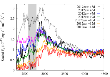
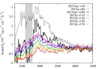
Figure 10: Early phase near-UV spectra of SN 2017eaw taken with the Swift UVOT/UGRISM instrument (black curves) compared to those of SN 2012aw (Bayless et al., 2013, left panel) and SN 2013ej (Dhungana et al., 2016, right panel). All spectra are dereddened and normalized to the same flux level in the 4000$-$4500Å regime. Note that the deep feature in the spectrum of SN 2017eaw at $\sim$2700 Å (marked by gray background color) is artificial due to contamination to the background level from a nearby stellar source.

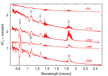
Figure 11: Near-IR spectra of SN 2017eaw obtained with NASA IRTF SpeX.

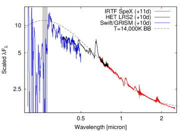
Figure 12: Simple fitting of a $T$=14 000K blackbody on a combined (near-UV-optical-near-IR) early-phase spectrum of SN 2017eaw. Contaminated region of the UV spectrum is marked by gray background color.

Comparison of the near-UV spectra of SN 2017eaw with those of two other Type II-P SNe, 2012aw and 2013ej, are presented in Fig. 10. Based on the findings of Gal-Yam et al. (2008), Type II-P SNe look very similar in the 2000$-$3000Å range; however, there are only a few objects with high-quality data. In the left panel of Fig. 10, we show the two near-UV spectra of SN 2017eaw together with the sequence of early-phase spectra of SN 2012aw (Bayless et al., 2013). All spectra are corrected for extinction and normalized to the same flux level between 4000 and 4500Å. Note that the strong flux depression in the +10d spectrum of SN 2017eaw is not real; it is due to contamination caused by the presence of 0th order images of nearby stars in the background region of the SN spectrum. Disregarding the contaminated region, the spectra of both SNe as well as their evolution are very similar, confirming the findings by Gal-Yam et al. (2008).

The right panel of Fig. 10 contains the same two near-UV spectra of SN 2017eaw, but compared to those of SN 2013ej (Dhungana et al., 2016). The similarity is less pronounced in this case, as SN 2017eaw appears to be relatively brighter than SN 2013ej between 2500 and 3500Å at +10d. As SN 2013ej was a “transitional” object between the Type II-P (“plateau”) and II-L (“linear”) SNe (Dhungana et al., 2016), such minor differences between the near-UV spectra are not unexpected and likely real.

Because all three SNe showed X-ray emission shortly after explosion (see Bayless et al., 2013; Chakraborti et al., 2016, as well as Sec. 4.2) that are consistent with the presence of very nearby CSM, the relatively lower near-UV flux of SN 2013ej is probably not due to the lack of early CSM-interaction. As SN 2013ej showed a shorter plateau than 2017eaw in its optical light curves (Dhungana et al., 2016), a faster spectral evolution, i.e. the faster decline of the near-UV flux in time, may be a more likely cause of the difference of its near-UV spectra with those of SNe 2017eaw.

The five near-IR spectra of SN 2017eaw, obtained with IRTF between +6 and +39 days, are plotted in Fig. 11. During the early phases, the spectra do not show many features; they are mostly dominated by the P Cygni profiles of the Ca II triplet and the hydrogen Paschen features. Nevertheless, the +6 and +11d IRTF spectra are the earliest near-IR spectra of SN 2017eaw published to date.

Moreover, the contemporaneous near-UV, optical, and near-IR spectra obtained at +10/11 days allowed us to make a well-constrained estimation for the photospheric temperature based on a wider wavelength range. We constructed a combined spectrum, which can be well fitted with a $T$=14,000K blackbody (see Fig. 12) – this value is in a good agreement with the photospheric temperature determined by Bose et al. (2013) from the spectral modeling of SN 2012aw at the same epoch.

Based on higher resolution spectra obtained with Gemini Near-Infrared Spectrograph between +22 and +205 days, Rho et al. (2018) carried out a more detailed analysis on SN 2017eaw. Their most important conclusion is that the spectra show the formation of a moderate amount of CO molecules and hot dust after $\sim$120 days. We will return to this finding in Section 4.3.

3.3 Distance estimates

The distance to SN 2017eaw and its host galaxy is estimated by combining the results from various methods, as detailed below.

3.3.1 Expanding Photosphere Method

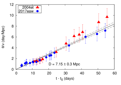
Figure 13: Distance determination from EPM applied to the combined SN 2017eaw + 2004et data (see text). The slope of the solid line gives $\sim D^{-1}$, and the dashed lines illustrate the effect of $\pm 0.3$ Mpc statistical uncertainty in the distance.

First, we apply the Expanding Photosphere Method (EPM) to the combined dataset of SN 2017eaw (this paper) and 2004et (Sahu et al., 2006; Misra et al., 2007; Maguire et al., 2010b). The photospheric velocities are derived from the absorption minima of $H\beta$ and the standard Fe II $\lambda 5169$ feature, as shown in the previous section. For the explosion dates we adopt JD 2,453,270.5 (Li et al., 2005) for SN 2004et and JD 2,457,886.5 for SN 2017eaw (see above).

Our method uses the combination of the light and velocity curves of two SNe that exploded within the same host galaxy. This technique has been applied for a number of cases recently: SN 2011dh & 2005cs in M51 (Vinkó et al., 2012), and SN 2013ej & 2002ap in M74 (Dhungana et al., 2016). The constraint that the distance must be the same for both SNe helps to overcome some of the issues related to the application of EPM to a single object, e.g. the sensitivity to the explosion date or stronger deviations from the modified blackbody evolution.

After correcting for the interstellar extinction using $E(B-V)_{tot}=0.41$ mag for the total reddening (see above) and assuming $R_{V}=3.1$ for the extinction law, we construct a quasi-bolometric LC for both SNe from their measured $BVRI$ data (see Section 3.5). Then we fit the standard equations of EPM (e.g. Vinkó et al., 2012) coupled with the dilution factors of Dessart & Hillier (2005) to the quasi-bolometric LCs simultaneously. The fit is restricted to the epochs $10<t<50$ days after explosion for several reasons. First, the LC of SN 2017eaw shows a bump at the earliest epochs (Fig. 4) that might be due to physical processes (e.g. CSM-interaction) that are not included in the simple physical model (an expanding blackbody) used in EPM. Also, at $t<10$ days the contribution from the UV-band flux, which is treated only approximately when assembling the quasi-bolometric LCs, is higher than at later phases. After $\sim 10$ days these complications seem to have less effect. After $t\sim 50$ days NLTE effects become increasingly dominant (see e.g. Dessart & Hillier, 2005), which also cause deviations from the simple blackbody approximation used in EPM. Thus, as a compromise, we fit the equations of EPM to data taken at $10<t<50$ days.

The result is shown in Figure 13. The slope of the line gives $D=7.15$ $\pm 0.30$ (statistical) $\pm 0.70$ (systematic) Mpc. The quoted systematic uncertainty comes from two main sources: a $\pm 1$ day uncertainty in the adopted explosion dates, and the sensitivity of the distance to the minimum and maximum epochs used in the EPM fitting. If we restrict the fitting to data taken in $0<t<30$ days, as recommended by Dessart & Hillier (2005), we get a $\sim 0.7$ Mpc higher common distance (see Table 2).

From Fig.13 it is seen that the data of the two SNe, even though they are consistent within the errors, start to deviate systematically from each other after $t>+30$ days. Thus, fitting the equations of EPM to only one of them would give different distances. Indeed, fitting only to SN 2004et, but also letting the moment of explosion ($t_{0}$) float, would result in $D\sim 5.23\pm 0.15$ Mpc and $t_{0}$ being $\sim 5$ days later than the assumed moment of explosion (see above), which is in conflict with the discovery date. Using SN 2017eaw only, the same analysis would give $D\sim 7.08\pm 0.11$ Mpc and $t_{0}\sim 1.9$ days later than assumed. These conflicting results illustrate why the fitting to the combined dataset (coupled with the constraints on the moment of explosion) can give more reliable results. Keeping in mind the uncertainties of reddening/extinction and the explosion date, this might explain why the previous applications of EPM to SN 2004et resulted in lower ($D\sim$5 Mpc) distances (see e.g. Takáts & Vinkó, 2012, and references therein).

Note that the application of the template velocity curve based on spectroscopic modeling by Takáts & Vinkó (2012) gives a distance that is only $\sim 0.1$ Mpc lower, thus, it is within the uncertainty of the fitting.

The results detailed above also depend on the assumed reddening ($E(B-V)_{tot}=0.41$). If we adopt only the reddening from the Milky Way dust, $E(B-V)\sim 0.3$ (Schlafly & Finkbeiner, 2011), and thus ignore the reddening within NGC 6946, then the EPM distance from the combined dataset would decrease to $D\sim 6.7$ Mpc. Given that dust in the host galaxy should also contribute somewhat to the total reddening, this is probably a lower limit, and the true distance is closer to $\sim$7 Mpc. Table 2 summarizes the distances derived above and also from other methods (see below).

Table 2: Distance estimates to NGC 6946

Method	Calibration	E(B-V)	D (Mpc)	$\sigma$ (Mpc)
EPM	A	0.41	7.15	0.3
EPM	A	0.30	6.66	0.3
EPM	B	0.41	7.85	0.2
EPM	B	0.30	6.93	0.4
SCM	C	–	6.69	0.3
SCM	D	–	6.69	0.2
SCM	E	–	6.02	0.3
TRGB	F	–	6.7	0.2
TRGB	G	–	7.7	0.3
PNLF	H	–	6.1	0.6
average			6.85	0.63

Notes. A) 10d$<t<$50d; B) 10d$<t<$30d ; C) Poznanski et al. (2009); D) de Jaeger et al. (2017), E) Gall et al. (2018); F) Tikhonov (2014); G) Anand et al. (2018); H) Herrmann et al. (2008).

3.3.2 Standard Candle Method

Second, we estimate the distance to SN 2017eaw by applying the Standard Candle Method (SCM). This method was first proposed by Hamuy & Pinto (2002), then it was refined and re-calibrated in various studies later (Takáts & Vinkó, 2006; Poznanski et al., 2009; Olivares et al., 2010; D’Andrea et al., 2010; Maguire et al., 2010a; de Jaeger et al., 2017; Gall et al., 2016).

For SN 2017eaw we measure $m_{V}(50)=13.20$, $m_{I}(50)=12.25$, $m_{r}(50)=12.77$, $m_{i}(50)=12.61$, $v_{FeII}(50)=4600\pm 200$ km s^-1 and $v_{H\beta}(50)=5350\pm 200$ km s^-1 for the $V$, $I$, $r$, and $i$-band magnitudes and expansion velocities at $t=50$d after explosion, respectively. Table 2 lists the distances of SN 2017eaw inferred from the three most recent SCM calibrations.

Compared to other distances listed in NED, most of which are based on using SCM on SN 2004et ($\sim 5$ Mpc), these new SCM-based distances to SN 2017eaw are all systematically higher. This is the same as found above when comparing the individual EPM-based distances of SNe 2017eaw and 2004et. The lower SCM-based distance to SN 2004et is due to the fact that SN 2004et showed brighter plateau, but lower expansion velocity at $t=50$d than SN 2017eaw. Indeed, from the data by Sahu et al. (2006) and Maguire et al. (2010b) we measure $m_{V}(50)=12.83$, $m_{I}(50)=11.93$, $v_{FeII}(50)=4230\pm 200$ km s^-1 and derive $D=5.43\pm 0.24$ Mpc from the calibration by Poznanski et al. (2009). If we correct the plateau brightness for Milky Way extinction ($E(B-V)=0.3$ mag) first and use these corrected magnitudes, then the SCM-based distance to SN 2004et decreases to $\sim 4.9\pm 0.2$ Mpc. Overall, the SCM-distances show the same trend as the EPM-based distances: they seem to be systematically higher for SN 2017eaw than for SN 2004et. This strengthens the suspicion that SN 2004et was not a typical Type II-P, thus, the previous distance estimates based on SN 2004et are probably biased.

3.3.3 Other distances to the host galaxy

NED also contains other redshift-independent distance estimates for NGC 6946 that are not related to SN data. In Table 2 we list the four most recent ones that are based on the “Tip of the Red Giant Branch” (TRGB) (Tikhonov, 2014; Anand et al., 2018) and the “Planetary Nebula Luminosity Function” (PNLF) (Herrmann et al., 2008) methods. The PNLF distance ($D\sim 6$ Mpc) is in between the ones derived for SN 2017eaw ($D\sim 7$ Mpc) and 2004et ($D\sim 5$ Mpc), while the other two are closer to that of SN 2017eaw.

We assign the average of the various distances listed in Table 2 to the final distance of NGC 6946, i.e. $D\sim 6.85$ $\pm 0.63$ Mpc (the quoted uncertainty is the rms error, but takes into account the uncertainties of the individual distances). This value disfavors the previous measurements from SN 2004et that all gave $\sim$30 percent lower distances. We use $D=6.85$ Mpc as the distance to SN 2017eaw in the rest of this paper.

3.4 Progenitor mass from nebular spectra

Observations taken during the nebular phase ($\sim$200-500 days post-explosion) reveal the inner nucleosynthetic products of the progenitor star and its explosive burning. The strength and shape of emission lines of individual elements can be mapped back to properties of the progenitor and explosion. In particular, a monotonic relation exists between the intensity of the [OI] doublet ($\rm{\lambda\lambda 6300,6364}$) and the mass of the progenitor star (Jerkstrand et al., 2012, 2014). We use this relationship to find the progenitor mass of SN 2017eaw using the spectra taken during the nebular phase.

We model the oxygen emission line using the suite of models presented in Jerkstrand et al. (2012) which are computed using the spectral synthesis code described in Jerkstrand, Fransson, & Kozma (2011). Model spectra are produced for $\rm{M_{ZAMS}=12,15,19,}$ and 25 $\rm{M_{\odot}}$ at epochs of 212, 250, 306, 400, and 451 days for the 12, 15, and 25 $\rm{M_{\odot}}$ models and at 212, 250, 332, 369, and 451 days for the 19 $\rm{M_{\odot}}$ model. These models were generated for SN 2004et using a nickel mass of $\rm{M_{{}^{56}Ni,mod}}$ = 0.062 $\rm{M_{\odot}}$ and $\rm{d_{mod}}$ = 5.5 Mpc. To apply these models to SN 2017eaw, the synthetic spectra are scaled to the inferred distance and nickel mass of SN 2017eaw via the following relation:

$$F_{obs}=F_{mod}\times\left(\frac{d_{mod}}{d_{obs}}\right)^{2}\left(\frac{M_{{}^{56}Ni,obs}}{M_{{}^{56}Ni,mod}}\right)e^{\frac{t_{mod}-t_{obs}}{111.4}}$$ (1)

where $\rm{F_{obs}}$ and $\rm{F_{mod}}$ are the observed and model fluxes, $\rm{d_{obs}}$ and $\rm{d_{mod}}$ are the observed and model distances, and $\rm{M_{{}^{56}Ni,obs}}$ and $\rm{M_{{}^{56}Ni,mod}}$ are the observed and model nickel masses synthesized during the explosion. Although SN 2004et and SN 2017eaw are in the same galaxy, we use the distance found in Section 3.3 as the distance to SN 2017eaw and scale the flux accordingly.

Using this method we find the progenitor mass to be 15 $\rm{M_{\odot}}$ for the first nebular spectrum and 12 $\rm{M_{\odot}}$ for the two later spectra. However, we find that the blue part of the continuum in the last two observed spectra is noticeably below the continuum in the models. For this reason, we scale the models empirically by the ratio of the integrated flux of the observed and model spectra. This produces a much better alignment of the continuum on the blue side of the spectrum and a consistent progenitor mass of $\sim 15$ $\rm{M_{\odot}}$ for all three spectra. The empirically scaled model spectra are plotted with the observed spectra in Figure 14. The inset in each panel shows the oxygen doublet in detail. As a sanity check, we use the empirical scale factor at each epoch and Equation 1 to compute the inferred nickel mass of SN 2017eaw. We find values of 0.025-0.036 $\rm{M_{\odot}}$ for the 15 $\rm{M_{\odot}}$ model, reasonably close to the value found in Section 3.5.

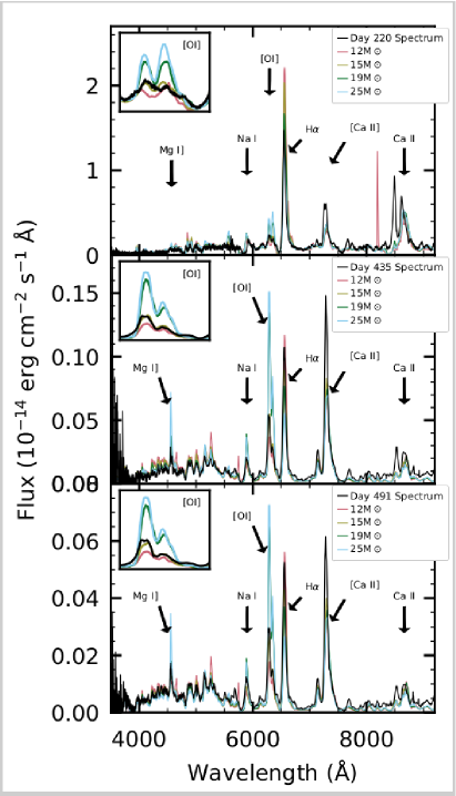
Figure 14: The nebular spectra of SN 2017eaw (black) observed 220 (top panel), 435 (middle panel), and 491 (bottom panel) days after explosion. The model spectra of Jerkstrand et al. (2012) are scaled by the integrated flux at each epoch such that the continuum of the observed spectrum and model spectrum are aligned for each 12 (pink), 15 (yellow), 19 (green), and 25 (blue) $\rm{M_{\odot}}$ progenitor. The [OI] line doublet ($\rm{\lambda\lambda 6300,6364}$) for the model and the observed spectra at each epoch is shown in the insets. The observed spectrum matches the 15 $\rm{M_{\odot}}$ model at all three epochs implying that this is the $\rm{M_{ZAMS}}$ of the progenitor.

3.5 Modeling the bolometric light curve

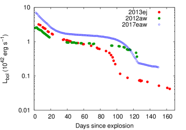
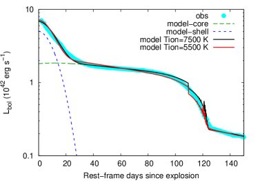
Figure 15: Left panel: The bolometric light curve of SN 2017eaw (including the UV-contribution from Swift) compared to that of SNe 2012aw (Bose et al., 2013) and 2013ej (Dhungana et al., 2016). Right panel: Fitting of two-component Arnett-Fu models (lines) to the bolometric light curve of SN 2017eaw (circles). The contributions from the“core” and the “shell” part of the ejecta are plotted with long- and short-dashed lines, respectively. The kink in the model light curves at the end of the plateau phase is a numerical artifact related to the finite resolution of the grid used to locate the recombination front.

Table 3: Parameters of the best-fit two-component Arnett-Fu models. See text for explanation. Parameters for SNe 2012aw and 2013 are adopted from Nagy & Vinkó (2016).

	SN 2017eaw		SN 2012aw	SN 2013ej
$T_{ion}$ (K)	$7,500$	$5,500$	$7,500$	$7,500$
”Core”
$R_{0}$ ($10^{13}$ cm)	3.3	2.0	2.9	2.9
$M_{\text{ej}}$ (M⊙)	14.3	14.6	20.0	10.0
$M_{\text{Ni}}$ (M⊙)	0.045	0.046	0.056	0.020
$E_{\text{tot}}$ (1051 erg)	2.70	4.87	2.20	1.45
$E_{\text{kin}}/E_{\text{th}}$	1.99	1.92	2.67	3.14
$\kappa$ (cm2 g-1)	0.24	0.24	0.13	0.20
$v_{\text{sc}}$ (km s-1)	4583	6033	3660	4290
$t_{\text{lc}}$ (d)	98.2	86.7	95.8	77.6
”Shell”
$R_{0}$ ($10^{13}$ cm)	4.9	4.5	4.5	6.8
$M_{\text{ej}}$ (M⊙)	0.37	0.33	1.0	0.6
$M_{\text{Ni}}$ (M⊙)	–	–	–	–
$E_{\text{tot}}$ (1051 erg)	0.18	0.20	1.0	1.39
$E_{\text{kin}}/E_{\text{th}}$	1.93	2.22	9.0	14.4
$\kappa$ (cm2 g-1)	0.34	0.34	0.40	0.40

The quasi-bolometric light curve, including the contributions from the UV and IR, is constructed by applying the same technique as described in Dhungana et al. (2016). After correcting the data for the total interstellar extinction (assuming $E(B-V)=0.41$ mag, see Sect. 3) and converting the magnitudes to physical fluxes, the SEDs are integrated along wavelength using the trapezoidal rule. Note that computing proper extinction correction for the Swift UV data is not as simple as for the optical data (Brown et al., 2010; Brown et al, 2016). Here we follow a somewhat simplified procedure by assuming constant extinction coefficients for the UVOT filters as determined by Brown et al. (2010) for the Type II-P SN 1999em (see their Table 14). The optical data are integrated between the B-band and the I-band, while the Swift data are used to compute the contribution between the B-band and 2000 Å. The integrated flux from the unobserved IR bands are taken into account by extrapolating the I-band fluxes with a Rayleigh-Jeans tail and integrating that curve to infinity. Finally, the integrated fluxes are corrected for distance using $D=6.85$ Mpc (Sect. 3.3). The resulting quasi-bolometric light curve is plotted together with those of SN 2012aw (Bose et al., 2013) and SN 2013ej (Dhungana et al., 2016) in Figure 15.

Radiation-diffusion models (Arnett & Fu, 1989; Fu & Arnett, 1989) for the bolometric light curve are computed with the LC2.2 code (Nagy & Vinkó, 2016) that assumes a two-component ejecta having an inner, denser, more massive envelope (referred to as the “core”, following Nagy & Vinkó, 2016) and an outer, less massive, lower density “shell”. The code takes into account H- or He-recombination in the same way as in Arnett & Fu (1989). More details on the physics of these models can be found in (Nagy & Vinkó, 2016). Briefly, the main difference between the two components is that the outer, low-density “shell” is assumed to be powered only by shock heating (and not by ⁵⁶Ni-decay).

The right panel in Figure 15 plots the observed bolometric light curve together with several models that are found to show similar luminosity evolution. The model parameters are listed in Table 3: the progenitor radius $R_{0}$ (in $10^{13}$ cm units), the mass of the ejecta ($M_{\text{ej}}$, in M_⊙), the initial mass of the radioactive ⁵⁶Ni ($M_{\text{Ni}}$, in M_⊙), the total energy ($E_{\text{tot}}$, in $10^{51}$ erg) and the ratio of the thermal ($E_{\text{th}}$) and kinetic energy ($E_{\text{kin}}$) of the ejecta, the opacity ($\kappa$, in cm² g^-1), the scaling velocity ($v_{\text{sc}}$, in km s^-1), and the light-curve timescale ($t_{\text{lc}}$, in days) (the geometric mean of the expansion and the diffusion timescales as defined by Arnett & Fu, 1989). The last two parameters are derived from the previous ones listed above.

The density profiles for all models are assumed to be constant as in Arnett & Fu (1989). The “shell” is assumed to be hydrogen-rich, thus, the usual $\kappa=0.34$ cm² g^-1 (which is equal to the Thompson-scattering opacity of a fully ionized solar-like plasma) is adopted as the opacity in this component. Since the “core” is more abundant in heavier elements, its Thompson-scattering opacity could be somewhat lower, thus, $\kappa\sim$0.24 cm² g^-1 is adopted there (Nagy, 2018). For the recombination temperature two different values ($T_{ion}=5500$ K and 7500 K) are assumed as lower and upper limits that roughly bracket the recombination temperature in a hydrogen-rich and a hydrogen-depleted atmosphere, respectively.

It has to be noted that, as it is described in detail in Nagy & Vinkó (2016), uncertainty of the explosion date can be a serious limitation during this modeling process; at the same time, the $\pm$1 day uncertainty in $t_{0}$ of SN 2017eaw (see Section 3) may cause only a $\sim$5% relative error in the derived physical parameters. Moreover, the mass estimate based on LC modeling has a well-known degeneracy with the assumed (constant) optical opacity and the kinetic energy; these parameters are correlated via the $t_{\text{lc}}$ parameter as $t_{\text{lc}}\sim\kappa M_{\text{ej}}^{3/2}E_{\text{kin}}^{-1/2}$. Thus, for the same light curve but a slightly different opacity than in Table 3 one can get different ejecta masses. For example, if using $\kappa=0.33$ cm² g^-1 in the “core” one would get a factor of 0.8 lower mass, i.e. $M_{\text{ej}}\sim 11$ M_⊙. Therefore, a more realistic estimate for the uncertainty of the derived ejecta mass is at least $\pm 3$ M_⊙, which takes into account the correlation between these key parameters.

In Table 3, parameters for SNe 2012aw and 2013ej calculated with the same two-component model (adopted from Nagy & Vinkó, 2016) are also shown. While slightly different opacities have been used during the modeling of the three SNe, the main parameters are similar. This suggests that the three progenitors were probably similar to each other. However, as can be also seen in Figure 15, the early-time bolometric fluxes are larger in the case of SN 2017eaw, which can be modeled with a higher total energy in the “core” (or, can be the sign of early-time CSM interaction). Further implications for the light curve models are discussed in Section 4.

4 Discussion

From the observations and models presented in the previous sections, we draw a comprehensive picture of SN 2017eaw, its progenitor and circumstellar environment.

4.1 Mass of the progenitor, explosion parameters

The model parameters shown in Table 3 imply a relatively, but not unusually massive Type II-P SN ejecta: the total (“core” + “shell”) envelope mass is $\sim 14.5\pm 3.0$ M_⊙. Assuming $\sim$1.4 M_⊙ for the mass of the remaining neutron star, this is in a good agreement with the progenitor mass of $\sim$15 M_⊙ inferred from our modeling of the nebular spectra (during which we used 12, 15, 19 and 25 M_⊙ models).

Tsvetkov et al. (2018) applied the multi-group radiation-hydro code STELLA (Blinnikov, 1998, 2000, 2006) to model their UBVRI light curves for SN 2017eaw. They obtained $R_{0}$ = 600 $R_{\odot}$ ($\sim$4.2 $\times 10^{13}$ cm), $M_{\text{ej}}$ = 23 $M_{\odot}$, $M_{\text{Ni}}$= 0.05 $M_{\odot}$, and $E_{\text{kin}}$= 2.0 foe, which are consistent with ours in Table 3. The only exception is their $\sim$1.5 times higher total ejecta mass. It is a well-known issue that radiation hydro codes sometimes give higher envelope masses than simple semi-analytic models (e.g Nagy & Vinkó, 2016). Given the uncertainties of the parameters from the semi-analytic models, which use a lot of approximations, such a difference within a factor of 2 is not unexpected. Note that our derived mass is more consistent with the mass estimates for the observed progenitor of SN 2017eaw ($14\pm 3$ M_⊙; van Dyk et al., 2017; Kilpatrick & Foley, 2018), as well as with the results of Rho et al. (2018) who compare their near-IR spectra with the models of Dessart et al. (2017, 2018) and conclude a progenitor mass of 15 M_⊙ (with M${}_{\text{ej}}$ of 12.5 M_⊙ and M${}_{\text{Ni}}$ of 0.084 M_⊙). Note also that Williams et al. (2018) give a much lower value for the progenitor mass ($\sim 8.8^{+2}_{-0.2}$ M_⊙) from modeling the local stellar population, but, from their Figure 2, this looks more like being a lower limit.

The initial “shell” radius of $\sim 4.5\times 10^{13}$ cm is in very good agreement with the conclusion by Kilpatrick & Foley (2018) that the progenitor of SN 2017eaw was a red supergiant (RSG) star.

4.2 Early-time circumstellar interaction, mass-loss of the progenitor

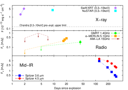
Figure 16: X-ray, radio and mid-IR data (together with published non-detections) of SN 2017eaw. Sources of data are listed in the text.

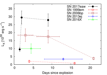
Figure 17: Early-time X-ray luminosities measured in Type II-P SNe: 2017eaw (0.3$-$10 keV), 1999em (0.4$-$8 keV, assuming a distance of $D$=12.5 Mpc, Pooley et al., 2002), 2006bp (0.4$-$8 keV, assuming a distance of $D$=14.9 Mpc, Immler et al., 2007), SN II-P/II-L 2013ej (0.5$-$8 keV, assuming a distance of $D$=9.57 Mpc, Chakraborti et al., 2016), and 2016X (0.3-10 keV, Grupe et al., 2016). For the latter three objects, horizontal error bars indicate the (not contiguous) periods covered by the observations.

Being one of the nearest SNe in the last decade, SN 2017eaw has been intensively followed up in both X-ray and radio bands in order to look for signs of possible early-time circumstellar interaction. Within only a day after discovery, the SN was positively detected in X-rays with Swift/X-Ray Telescope (XRT) at two different epochs, showing a significant early brightening in the 0.3-10 keV range by Kong & Li (2017), who also gave a (much lower) pre-explosion upper flux limit based on archival Chandra images of the SN site. A few days later the SN was also observed with the Nuclear Spectroscopic Telescope Array (NuSTAR) telescope (Grefensetette et al., 2017), detecting a slightly lower flux between 0.3-10 keV than previously found by Swift. Moreover, the latter authors also reported the presence of a line from ionized Fe around 6.65 keV, which implies the presence of shock-heated ejecta. Unfortunately, no further X-ray observations have been published to date; however, the SN has been also detected with the AstroSat/UV Imaging Telescope (UVIT) in the far-UV channel $\sim 2$ weeks after explosion (Misra et al., 2017).

The top panel of Fig. 16 presents all the published X-ray fluxes measured for SN 2017eaw. Using the distance of $D$=6.85 Mpc (see above), we determined the integrated unabsorbed X-ray luminosities for SN 2017eaw in the 0.3$-$10 keV range as $L_{X}$= 9.5$\times$10³⁸, 29.5$\times$10³⁸, and 27.9$\times$10³⁸ erg s^-1 at +1.5d, +2d and +9d, respectively.

In order to compare these X-ray luminosities with those of other Type II-P SNe, we have collected the available data from the literature. There are only a few SNe II-P that were observed in X-rays at such early phases. Fig. 17 shows the X-ray luminosities ($L_{X}$) of SN 2017eaw, together with that of SNe 1999em (Pooley et al., 2002), 2006bp (Immler et al., 2007), the Type II-P/II-L 2013ej (Chakraborti et al., 2016) and 2016X (Grupe et al., 2016). It is seen that the $L_{X}$ for SN 2017eaw (measured in the 0.3$-$10 keV range) is a few times higher than that of SNe 2006bp and 2016X and much higher than for SNe 1999em and 2013ej (however, the latter objects were observed only in the 0.4/0.5$-$8 keV range). Note that if we use $D\sim$5 Mpc for the distance of SN 2017eaw, we get $\sim$50% lower $L_{X}$ values, which are at the same level as that of SN 2006bp but are still much larger than other published values regarding Type II-P SNe. We also note that SN 2013fs was also followed up by Swift/XRT in the first $\sim$25 days, and a combined upper limit of $L_{X}<$4.7 $\times$ 10⁴⁰ erg s^-1 was determined by Yaron et al. (2017); however, as those authors noted, most of the estimated flux may originate from the host galaxy instead of the SN, because of the relatively large distance.

While the level of the early-time X-ray emission measured in SN 2017eaw is much lower than usually found in Type IIn or other strongly interacting SNe (see e.g. Chevalier & Fransson, 2017), its origin can be best explained by assuming a moderate interaction between the SN shock and the ambient circumstellar medium. As showed by, e.g., Immler et al. (2007) in the case of SN 2006bp, other possible sources (radioactive decay products of the ejecta, or inverse Compton scattering of photospheric photons off relativistic electrons produced by the explosion) can be responsible for only a fraction of the observed X-ray emission.

Regarding radio observations, all the early notifications reported non-detections at 1.4, 5.1, and 15 GHz (Nayana & Chandra, 2017a; Argo et al., 2017a; Bright et al., 2017; Mooley et al., 2017). Later, subsequent observations at the two lower frequencies resulted in positive detections: on three epochs between +17-20 days at 5.1 GHz (using e-MERLIN, Argo et al., 2017b), and at +42 days at 1.4 GHz (using Giant Metrewave Radio Telescope, GMRT, Nayana & Chandra, 2017b). All of these data are shown in the middle panel of Fig. 16. Since there are only a few observations of SN 2017eaw (obtained at three different frequencies), detailed modeling of the radio LCs can not be accomplished. Nevertheless, the estimated radio luminosities at 5.1 GHz are $\sim$10²⁶ erg s^-1 Hz^-1, which agree well with the peak luminosities of other Type II-P SNe assumed to go through moderate CSM interaction (see e.g. Chevalier et al., 2006).

Beyond X-ray and radio data, optical LCs may also indicate the presence of early-time CSM interaction. As has been found by Moriya et al. (2011, 2017, 2018) and Morozova et al. (2017, 2018), the mass-loss processes of the presumed RSG progenitors may significantly affect the optical LCs of Type II(-P) SNe, especially during the first few days. As mentioned in Section 3.1 and seen in Fig.4, SN 2017eaw shows a low-amplitude, early bump peaking at $\sim$6-7 days after explosion in the optical bands (most obviously in the I-band and weakening toward shorter wavelengths). This phenomenon is quite similar to the one observed in SN 2013fs, and is supposed to be caused by the interaction between the expanding SN ejecta and the ambient matter originating from the pre-explosion RSG wind.

There is a long-term debate on the amount, density distribution and geometry of the circumstellar material surrounding SN progenitors, as well as on the pre-explosion mass-loss history of RSG stars. In the basic (perhaps simplistic) framework, RSG stars have slow ($v_{\text{w}}\sim$10$-$20 km s^-1), steady winds resulting in mass loss rates ($\dot{M}$) of 10${}^{-6}-$10${}^{-5}M_{\odot}$ yr^-1. At the same time, mass loss may become enhanced just before the explosion, resulting in a (more or less) compact and dense inner region in the CSM: $\dot{M}\sim$ 10${}^{-4}-$10${}^{-2}M_{\odot}$ yr^-1 and $R\sim 10^{4}R_{\odot}$ (Moriya et al., 2011, 2017, 2018), or, even $\dot{M}\sim$ 10${}^{-2}-$15 $M_{\odot}$ yr^-1 and $R\sim 2000-3000R_{\odot}$ (Morozova et al., 2017, 2018). On the other hand, it is also possible that the shock simply breaks out from a very extended RSG atmosphere; in this case the “superwind” description may not be adequate (see e.g. Dessart et al., 2017).

In the case of SN 2017eaw, Kilpatrick & Foley (2018) carried out a detailed investigation on the pre-explosion environment of the assumed progenitor using archived HST and Spitzer data (see above). They suggested the presence of a low-mass ($M>2\times 10^{-5}M_{\odot}$), extended ($R=4000R_{\odot}$) dust shell enshrouding the progenitor site. They also estimated the mass-loss rate by applying the method of Kochanek et al. (2012) and obtained $\dot{M}\sim 9\times 10^{-7}M_{\odot}$ yr^-1.

Applying the method described in Kochanek et al. (2012) (adopted from Chevalier & Fransson, 2003), and using the parameters of our two LC models in Table 3 combined with the X-ray luminosities ($L_{X}$) given above we can derive another constraint for $\dot{M}$ via Eq. 4 of Kochanek et al. (2012),

$$L_{X}\simeq 1.63\times 10^{7}E_{51}^{27/20}M_{e10}^{-21/20}\dot{M}_{-4}^{7/10}v_{\text{w}10}^{-7/10}$$

$$\times t_{1}^{-3/10}L_{\odot},$$ (2)

where the total energy of the SN is $E=10^{51}E_{51}$ ergs, the ejected mass is $M_{ej}=10M_{e10}M_{\odot}$, $\dot{M}=10^{-4}\dot{M}_{-4}M_{\odot}\text{yr}^{-1}$, $v_{\text{w}}=10v_{\text{w}10}$ km s^-1, and $t_{1}$ is the elapsed time in days (+5 and +9 days in this case).

Assuming $v_{\text{w}1}$= 10 km s^-1 for the RSG wind velocity, we got $\dot{M}\sim 3\times 10^{-7}$ and $\sim$1 $\times 10^{-6}M_{\odot}$ yr^-1 for the two models listed in Table 3. Both of these values are consistent with the mass-loss rate estimated by Kilpatrick & Foley (2018). On the other hand, they are orders of magnitude lower than the mass-loss rates estimated by Moriya et al. and Morozova et al. via LC-modeling, or the value of $\dot{M}\sim$10${}^{-3}M_{\odot}$ yr^-1 derived by Yaron et al. (2017) for SN 2013fs based on modeling the early-time spectroscopic emission features. We note that from Eq. 2 it would be necessary to have $L_{X}\sim$10⁴¹ erg s^-1 to get $\dot{M}\sim$10${}^{-3}M_{\odot}$ yr^-1 for the mass-loss rate of SN 2017eaw. Such high-level X-ray luminosity has been measured only in strongly interacting SNe IIn to date.

Nevertheless, while it seems to be a serious contradiction, some caveats in the above analysis must be mentioned. First, the mass-loss rate we estimated from X-ray luminosities (beyond the intrinsic uncertainties of the model) is based on the assumption that the dominating counterpart of $L_{X}$ is the cooling of the reverse shock and its softer emission dominates the observable X-ray flux; however, as Grefensetette et al. (2017) noted, the analysis of the +9d X-ray spectrum of SN 2017eaw indicates a hard X-ray spectrum having detectable flux up to 30 keV (they also mention that the contribution of the 10-30 keV counterpart to the total $L_{X}$ is $<$10 percent). Second, the radius of the dust-rich pre-explosion region ($\sim 4000R_{\odot}$) derived by Kilpatrick & Foley (2018) is in good agreement with the general estimation given by Morozova et al. (2017, 2018) for the size of the cocoons of CSM around SNe II-P; the only difference is that the latter authors suggest the presence of a much denser environment. Signs of such a dense gas/dust shell are not seen in the combined optical-IR SED of the assumed progenitor of SN 2017eaw. High-resolution near-IR spectroscopy also did not detect narrow lines that may be an indication of CSM gas (see Rho et al., 2018). However, it is also true that these data do not cover the region of cold ($T\lesssim$ 300K) dust. Third, a common problem is the geometry; while the models generally assume a spherically symmetric CSM, it may also take the form of a thick disk, or a more complex structure of the inflated RSG envelope material (see e.g. Dessart et al., 2017; Morozova et al., 2017, and references therein). The actual shape of the CSM cloud may also have a strong influence on the estimated parameters. All of these uncertainties point toward the need for further observations and more detailed modeling in order to better understand the role of nearby CSM around Type II-P SNe as well as the mass-loss history of their RSG progenitors.

Moreover, it is also an intriguing question why we did not see any narrow (“flash-ionized”) emission lines in the earliest spectra of SN 2017eaw, unlike in the early ($<$5d) spectra of SN 2013fs and several other interacting Type II SNe (Quimby et al., 2006; Khazov et al., 2016; Yaron et al., 2017). While this problem also requires further data and modeling, the geometry and/or clumpiness of the CSM may also play a role here.

4.3 Possible signs of late-time dust formation

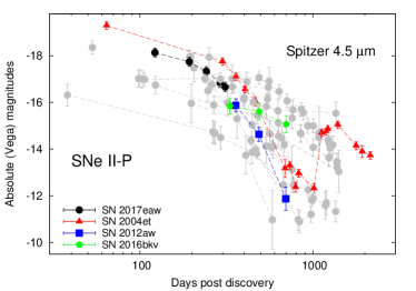
Figure 18: Mid-IR evolution of SN 2017eaw compared to that of other normal (gray) or interacting Type II-P SNe. 4.5 $\mu$m magnitudes of SNe 2017eaw and 2016bkv come from this work, while the source of other values is Szalai et al. (2018).

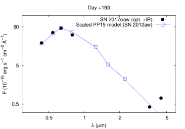
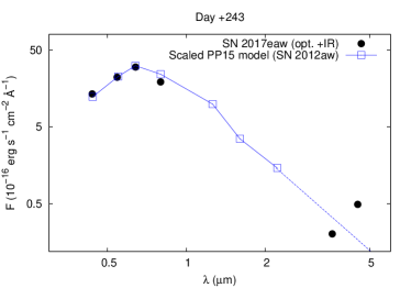
Figure 19: Optical-IR combined SED of SN 2017eaw (filled circles) compared to the scaled model SEDs of SN 2012aw calculated from Pejcha & Prieto (2015) (PP15) (open rectangles).

SN 2017eaw was also followed by Spitzer as the target of two different programs (PID 13239, PI: K. Krafton; PID 13053/SPIRITS, PI: M. Kasliwal). We have downloaded the public data from the Spitzer Heritage Archive (SHA) and carried out simple aperture photometry on post-basic calibrated (PBCD) images. The SN appears as a bright, continuously fading object in both IRAC 3.6 and 4.5 $\mu$m channels. We present the results from our photometry at the bottom panel of Fig. 16, while Fig. 18 shows the 4.5 $\mu$m light curve of SN 2017eaw compared to those of other Type II-P SNe (most of these data are adopted from Szalai et al., 2018, and references therein, while for SN 2016bkv we carried out a similar process as above).

During the observed period, the mid-IR evolution of SN 2017eaw seems to be similar to that of the highlighted Type II-P events (SNe 2004et, 2012aw, 2016bkv) that do not show strong, direct signs of dust formation (e.g. re-brightening in the mid-IR after several hundred days). At the same time, comparing the combined optical-IR SEDs of SN 2017eaw taken at +193d and +243d (Fig.19) to model SEDs of SN 2012aw (Pejcha & Prieto, 2015) there is a clear mid-IR excess in the 4.5 $\mu$ channel on both epochs. Here we note that in Type II-P SNe the 4.5 $\mu$m flux may also be contaminated by the 1$-$0 vibrational band of CO at 4.65 $\mu$m, which can influence the SED modeling at epochs $\lesssim$500d (see e.g. Kotak et al., 2005; Szalai et al., 2011).

These results seem to strengthen that of Rho et al. (2018), who, based on the detailed analysis of ground-based near-IR spectra, suggest ongoing (moderate) molecule (CO) and dust formation between $\sim$125-205 days. A more detailed study of dust and molecule formation in SN 2017eaw has been very recently published by Tinyanont et al. (2019); based on the analysis of the full Spitzer data set and near-IR photometry and spectroscopy up to $\sim$550d, these authors present similar conclusions to ours. We also note that, as can be seen, e.g., in the case of SN 2004et in Fig. 18, dust formation can become more significant at later times ($\sim$800$-$1000d after explosion), probably due to an interaction between the forward shock and a denser CSM shell (see e.g. Szalai et al., 2018, and references therein).

5 Conclusions

SN 2017eaw, one of the most nearby supernovae to appear in this decade, is a Type II-P explosion that shows early-time, moderate CSM interaction. We made a comprehensive study of this SN using multi-colour optical photometry and high-quality optical spectroscopy starting at very early epochs and extending into the early nebular phase, near-UV and near-IR spectra, early-time X-ray and radio detections, and late-time mid-IR photometry.

We derived a new distance to the host galaxy, NGC 6946, after combining various distance estimates including the EPM analysis of the combined data of SNe 2017eaw and 2004et. The final distance, $D\sim 6.85$ $\pm 0.63$ Mpc, disfavors the previous measurements from SN 2004et only that all gave $\sim$30 percent lower distances.

During the whole period covered by the observations, the evolution of SN 2017eaw seems to be similar to those of some other “normal” Type II-P SNe (2004et, 2012aw). However, SN 2017eaw shows a small, early bump peaking at $\sim$6-7 days after explosion in all optical bands, which resembles the early light curve of SN 2013fs and is presumably the sign of early-time circumstellar interaction. Nevertheless, it is an intriguing question why we did not see any narrow (“flash-ionized”) emission features in the earliest optical spectra of SN 2017eaw; the solution of this problem might be related to different geometries and/or clumpiness of CSM around the two objects.

We modeled the quasi-bolometric LC of SN 2017eaw using a two-component radiation-diffusion model and estimated the basic physical parameters of the explosion and the ejecta. We also carried out modeling of the nebular spectra using different progenitor masses. The results agree well with the previous findings of a RSG progenitor star with a mass of $\sim$15-16 M_⊙.

We also used these calculated explosion parameters – together with early-phase X-ray luminosities – to derive the mass-loss rate of the progenitor. We got $\dot{M}\sim 3\times 10^{-7}-$ $1\times 10^{-6}M_{\odot}$ yr^-1; these values agrees well with that estimated by Kilpatrick & Foley (2018) based on the opacity of the dust shell enshrouding the progenitor, but it is orders of magnitude lower than the generally estimated values for Type II-P SNe from from early-phase LC modeling (Moriya et al., 2011, 2017, 2018; Morozova et al., 2017, 2018). We discussed several factors that may seriously influence the various estimations of $\dot{M}$ including the limitations within the models as well as the simplifying assumptions on the geometry and clumpiness of the nearby CSM.

Finally, we also studied the available mid-IR data of SN 2017eaw. The combined optical-IR SEDs show a clear mid-IR excess at +193 and +243 days, which are consistent with the results of Rho et al. (2018) and Tinyanont et al. (2019) on the (moderate) dust formation in the vicinity of this SN.

Appendix A Photometric and spectroscopic data

Table A1: Konkoly BVRI photometry of SN 2017eaw

Date	Epoch	B	$\sigma$B	V	$\sigma$V	R	$\sigma$R	I	$\sigma$I
(MJD)	(days)	(mag)	(mag)	(mag)	(mag)	(mag)	(mag)	(mag)	(mag)
57887.99	1.99	13.270	0.028	13.066	0.022	12.812	0.016	12.629	0.013
57889.83	3.83	13.202	0.032	12.886	0.031	12.567	0.026	12.340	0.012
57890.84	4.84	13.156	0.030	12.843	0.026	12.488	0.047	12.237	0.048
57892.00	6.00	13.204	0.045	12.848	0.040	12.448	0.033	12.184	0.026
57892.98	6.98	13.186	0.022	12.796	0.024	12.405	0.028	12.165	0.023
57894.95	8.95	13.170	0.014	12.830	0.021	12.398	0.034	12.165	0.019
57897.90	11.90	13.280	0.018	12.885	0.019	12.460	0.016	12.224	0.017
57898.96	12.96	13.305	0.021	12.915	0.021	12.470	0.028	12.245	0.016
57900.90	14.90	13.405	0.026	12.957	0.026	12.490	0.024	12.294	0.025
57901.90	15.90	13.431	0.026	12.951	0.026	12.502	0.024	12.294	0.025
57902.90	16.90	13.475	0.026	12.983	0.026	12.508	0.025	12.286	0.025
57904.90	18.90	13.531	0.028	12.976	0.027	12.507	0.025	12.277	0.026
57905.90	19.90	13.559	0.007	12.959	0.006	12.491	0.005	12.262	0.005
57906.90	20.90	13.623	0.006	12.962	0.006	12.490	0.004	12.263	0.005
57907.90	21.90	13.628	0.008	12.979	0.007	12.494	0.005	12.257	0.005
57909.90	23.90	13.765	0.008	12.989	0.007	12.491	0.005	12.254	0.006
57912.90	26.90	13.919	0.010	13.011	0.007	12.522	0.005	12.286	0.006
57913.90	27.90	13.905	0.010	13.049	0.007	12.538	0.005	12.258	0.005
57915.00	29.00	13.964	0.008	13.066	0.006	12.547	0.005	12.286	0.005
57915.90	29.90	14.006	0.008	13.071	0.006	12.557	0.005	12.269	0.005
57916.90	30.90	14.054	0.011	13.087	0.008	12.561	0.006	12.272	0.006
57917.90	31.90	14.070	0.009	13.105	0.007	12.566	0.005	12.279	0.005
57918.94	32.94	14.135	0.063	13.109	0.035	12.569	0.036	12.275	0.035
57919.99	33.99	14.116	0.008	13.123	0.006	12.590	0.004	12.274	0.005
57922.00	36.00	14.197	0.011	13.106	0.010	12.603	0.007	12.300	0.008
57924.00	38.00	14.252	0.008	13.187	0.006	12.610	0.005	12.297	0.005
57925.95	39.95	14.301	0.010	13.176	0.006	12.620	0.005	12.277	0.005
57927.90	41.90	14.327	0.009	13.194	0.008	12.620	0.005	12.286	0.006
57929.02	43.02	14.375	0.010	13.199	0.007	12.622	0.005	12.281	0.005
57931.00	45.00	14.425	0.054	13.209	0.039	12.611	0.022	12.258	0.024
57937.86	51.86	14.486	0.023	13.230	0.022	12.628	0.015	12.261	0.023
57940.90	54.90	14.558	0.038	13.222	0.028	12.622	0.020	12.239	0.020
57942.91	56.91	14.563	0.044	13.229	0.039	12.617	0.023	12.245	0.021
57945.90	59.90	14.605	0.070	13.231	0.030	12.627	0.027	12.238	0.034
57947.90	61.90	14.595	0.059	13.240	0.027	12.627	0.033	12.240	0.031
57951.92	65.92	14.632	0.030	13.262	0.020	12.638	0.010	12.235	0.010
57952.90	66.90	14.627	0.010	13.270	0.007	12.637	0.005	12.235	0.005
57956.90	70.90	14.717	0.046	13.297	0.038	12.626	0.031	12.235	0.024
57957.94	71.94	14.723	0.063	13.300	0.041	12.655	0.034	12.231	0.028
57959.87	73.87	14.738	0.055	13.299	0.035	12.643	0.033	12.238	0.028
57961.96	75.96	14.770	0.023	13.292	0.020	12.626	0.023	12.226	0.018
57962.86	76.86	14.810	0.037	13.297	0.033	12.636	0.029	12.233	0.019
57964.86	78.86	14.797	0.008	13.325	0.005	12.657	0.003	12.252	0.004
57965.94	79.94	14.818	0.008	13.333	0.005	12.675	0.003	12.245	0.004
57966.92	80.92	14.821	0.008	13.332	0.005	12.669	0.003	12.257	0.004
57967.87	81.87	14.858	0.062	13.376	0.032	12.660	0.034	12.257	0.019
57968.88	82.88	14.888	0.025	13.356	0.026	12.658	0.027	12.235	0.039
57970.89	84.89	14.905	0.064	13.382	0.033	12.693	0.025	12.268	0.022
57972.88	86.88	14.961	0.038	13.417	0.021	12.692	0.014	12.282	0.020
57973.86	87.86	14.977	0.046	13.410	0.025	12.692	0.022	12.278	0.020
57974.86	88.86	14.989	0.041	13.422	0.030	12.716	0.018	12.291	0.025
57976.00	90.00	15.011	0.046	13.422	0.016	12.727	0.024	12.294	0.014
57980.02	94.02	15.117	0.041	13.523	0.032	12.766	0.028	12.349	0.030
57982.84	96.84	15.192	0.031	13.555	0.028	12.778	0.029	12.367	0.021
57983.85	97.85	15.229	0.032	13.583	0.019	12.813	0.029	12.383	0.023
57986.86	100.86	15.340	0.034	13.648	0.019	12.874	0.019	12.437	0.016
57987.92	101.92	15.337	0.012	13.694	0.007	12.909	0.004	12.466	0.004
57988.84	102.84	15.418	0.032	13.718	0.024	12.923	0.023	12.484	0.021
57993.81	107.81	15.647	0.042	13.925	0.024	13.088	0.020	12.622	0.025
57994.88	108.88	15.768	0.059	13.980	0.044	13.136	0.031	12.673	0.033
57995.88	109.88	15.818	0.058	14.051	0.043	13.178	0.022	12.700	0.018
58000.83	114.83	16.202	0.068	14.384	0.030	13.470	0.016	12.963	0.048
58006.81	120.81	16.880	0.056	15.084	0.032	14.051	0.035	13.505	0.025
58011.80	125.80	17.385	0.048	15.530	0.027	14.434	0.019	13.858	0.020
58022.92	136.92	17.779	0.048	15.679	0.031	14.561	0.019	14.024	0.011
58023.92	137.92	17.540	0.037	15.698	0.029	14.603	0.030	14.048	0.019
58024.82	138.82	17.617	0.037	15.725	0.026	14.617	0.022	14.049	0.019
58025.80	139.80	17.564	0.041	15.754	0.021	14.620	0.024	14.053	0.021
58026.88	140.88	17.672	0.015	15.761	0.011	14.655	0.015	14.048	0.012
58027.83	141.83	17.648	0.022	15.816	0.009	14.677	0.019	14.076	0.013
58032.75	146.75	17.615	0.025	15.809	0.024	14.695	0.008	14.099	0.006
58035.75	149.75	17.661	0.019	15.886	0.009	14.736	0.011	14.143	0.013
58040.81	154.81	17.684	0.044	15.899	0.025	14.818	0.026	14.211	0.020
58041.84	155.84	17.679	0.012	15.916	0.013	14.781	0.011	14.181	0.011
58044.79	158.79	17.678	0.056	15.906	0.027	14.828	0.029	14.217	0.022
58046.72	160.72	17.798	0.035	15.944	0.025	14.815	0.025	14.258	0.015
58050.70	164.70	17.771	0.047	15.973	0.024	14.884	0.017	14.276	0.021
58055.95	169.95	17.768	0.038	16.069	0.026	14.871	0.017	14.314	0.023
58063.89	177.89	17.901	0.018	16.131	0.015	14.964	0.010	14.364	0.008
58064.81	178.81	17.841	0.031	16.139	0.023	14.948	0.006	14.368	0.006
58075.80	189.80	17.874	0.072	16.221	0.031	15.110	0.031	14.729	0.064
58094.79	208.79	18.083	0.054	16.407	0.030	15.235	0.025	14.674	0.028
58182.12	296.12	18.659	0.077	17.330	0.046	16.191	0.031	15.620	0.027

Table A2: LCO UBV$g^{\prime}r^{\prime}i^{\prime}$ photometry of SN 2017eaw

Date	Epoch	U	B	V	$g^{\prime}$	$r^{\prime}$	$i^{\prime}$
(MJD)	(days)	(mag)	(mag)	(mag)	(mag)	(mag)	(mag)
57888.85	2.85	12.523(.014)	13.222(.012)	12.992(.022)	12.760(.018)	12.903(.013)	12.880(.023)
57889.91	3.91	–	13.198(.011)	12.888(.015)	12.698(.010)	12.774(.012)	12.752(.015)
57891.93	5.93	12.431(.012)	13.148(.019)	12.807(.016)	12.653(.018)	12.653(.019)	12.573(.015)
57893.82	7.82	12.394(.025)	13.128(.007)	12.774(.015)	12.656(.022)	12.591(.024)	12.500(.012)
57895.91	9.91	–	13.146(.009)	12.855(.022)	12.699(.012)	12.612(.016)	12.556(.035)
57896.89	10.89	12.467(.018)	13.173(.014)	12.868(.013)	12.703(.020)	12.580(.010)	12.542(.010)
57897.81	11.81	–	13.229(.012)	12.869(.022)	12.731(.011)	12.593(.016)	12.557(.016)
57898.83	12.83	12.655(.017)	13.257(.017)	12.888(.011)	12.769(.015)	12.613(.012)	12.583(.018)
57902.81	16.81	12.886(.012)	13.374(.038)	12.933(.029)	12.862(.015)	12.634(.011)	12.620(.014)
57906.82	20.82	–	13.476(.022)	12.945(.013)	12.868(.019)	12.582(.023)	12.619(.046)
57907.86	21.86	13.344(.013)	13.536(.019)	12.868(.013)	12.911(.032)	12.583(.010)	12.555(.023)
57908.87	22.87	13.491(.035)	13.581(.020)	12.924(.011)	12.939(.027)	12.597(.011)	12.535(.018)
57909.85	23.85	13.601(.034)	13.638(.011)	12.920(.010)	12.977(.010)	12.608(.025)	12.596(.011)
57910.88	24.88	–	–	12.995(.010)	12.984(.023)	12.643(.015)	12.600(.019)
57916.89	30.89	–	–	–	13.178(.011)	12.669(.018)	12.593(.010)
57917.84	31.84	–	13.981(.014)	13.037(.014)	13.200(.011)	12.673(.018)	12.586(.012)
57928.79	42.79	14.879(.030)	14.281(.017)	13.169(.015)	13.418(.010)	12.782(.010)	12.685(.010)
57934.82	48.82	15.146(.030)	14.373(.026)	13.164(.014)	13.477(.015)	12.769(.032)	12.614(.029)
57940.84	54.84 15.426(.019)	14.447(.012)	13.159(.012)	13.448(.010)	12.774(.014)	12.611(.016)
57944.80	58.80	15.493(.018)	14.513(.015)	13.193(.011)	13.524(.012)	12.791(.008)	–
57945.84	59.84	15.522(.023)	14.543(.016)	13.185(.014)	13.552(.013)	12.805(.018)	12.606(.025)
57961.83	75.83	16.014(.051)	14.699(.018)	13.221(.011)	13.683(.012)	12.821(.011)	12.640(.015)
57965.93	79.93	–	14.834(.054)	–	–	–	–
57971.87	85.87	16.425(.047)	14.902(.016)	13.340(.012)	13.789(.013)	12.850(.018)	12.625(.026)
57972.83	86.83	16.392(.037)	14.902(.014)	13.345(.014)	13.831(.020)	12.875(.013)	12.668(.005)
57976.80	90.80	16.641(.016)	15.015(.018)	13.408(.019)	13.901(.036)	12.979(.023)	12.716(.013)
57995.81	109.81	17.756(.028)	15.747(.027)	13.907(.038)	14.593(.012)	13.315(.019)	13.055(.013)
58001.74	115.74	–	16.267(.018)	14.430(.012)	15.095(.028)	13.716(.012)	13.410(.026)
58002.84	116.84	–	16.375(.039)	14.489(.016)	15.158(.017)	13.777(.018)	13.513(.017)
58004.81	118.81	–	16.629(.017)	14.768(.022)	15.403(.026)	13.974(.011)	13.678(.016)
58005.82	119.82	–	16.719(.043)	14.868(.013)	15.589(.015)	14.099(.013)	13.834(.012)
58008.82	122.82	–	17.123(.022)	15.289(.021)	15.935(.036)	14.405(.018)	14.131(.048)
58009.80	123.80	–	17.247(.028)	15.379(.018)	–	–	–
58010.83	124.83	–	17.334(.016)	15.395(.011)	16.136(.012)	14.597(.015)	14.287(.028)
58018.78	132.78	–	17.535(.026)	15.651(.015)	16.361(.015)	14.793(.027)	14.481(.013)
58019.77	133.77	–	17.502(.014)	15.669(.024)	16.383(.017)	14.786(.014)	14.457(.022)
58028.75	142.75	–	17.611(.023)	15.756(.022)	16.444(.015)	14.838(.010)	14.557(.006)
58034.76	148.76	–	17.710(.025)	15.823(.037)	16.450(.030)	14.900(.018)	14.645(.025)
58035.73	149.73	–	17.630(.028)	15.781(.022)	16.495(.021)	14.884(.012)	14.668(.021)
58039.75	153.75	–	17.687(.017)	15.831(.012)	16.583(.010)	14.960(.011)	14.722(.041)
58043.73	157.73	–	17.703(.013)	15.868(.014)	16.588(.013)	14.992(.018)	14.735(.012)
58047.60	161.60	–	17.710(.019)	15.929(.013)	–	–	–
58051.62	165.62	–	17.747(.034)	15.970(.020)	16.674(.010)	15.038(.020)	14.809(.013)
58055.59	169.59	–	17.801(.029)	16.028(.020)	16.679(.010)	15.096(.028)	14.833(.014)
58059.66	173.66	–	17.824(.023)	16.061(.010)	16.681(.011)	15.088(.020)	14.882(.015)
58060.65	174.65	–	17.760(.029)	16.032(.010)	16.679(.018)	15.114(.012)	14.900(.012)
58071.62	185.62	–	17.843(.112)	16.045(.036)	16.809(.016)	15.132(.028)	14.977(.013)
58082.57	196.57	–	17.955(.023)	16.298(.015)	16.880(.016)	15.302(.018)	15.132(.020)
58099.57	213.57	–	17.997(.022)	16.449(.029)	16.984(.015)	15.460(.011)	15.301(.015)
58231.02	345.02	–	19.012(.033)	17.819(.014)	18.064(.013)	16.933(.025)	16.623(.017)
58246.05	360.05	–	–	17.984(.026)	18.167(.021)	17.136(.019)	16.820(.046)
58246.83	360.83	–	19.065(.040)	17.958(.060)	18.153(.029)	17.131(.062)	16.793(.018)
58255.02	369.02	–	19.134(.014)	18.030(.010)	18.249(.026)	17.245(.037)	16.906(.031)
58258.81	372.81	–	19.180(.023)	18.086(.011)	18.326(.022)	17.374(.028)	16.986(.010)
58267.92	381.92	–	–	18.253(.027)	18.487(.038)	17.466(.034)	17.142(.051)
58284.78	398.78	–	19.453(.018)	18.354(.014)	18.632(.015)	17.666(.044)	17.345(.041)
58292.77	406.77	–	19.521(.032)	18.506(.034)	–	17.769(.013)	17.390(.016)
58318.75	432.75	–	19.783(.021)	18.784(.011)	18.909(.048)	18.175(.017)	17.768(.022)
58335.90	449.90	–	19.976(.059)	19.045(.022)	19.204(.033)	18.381(.019)	–
58351.74	465.74	–	20.092(.086)	19.230(.013)	19.397(.047)	18.631(.023)	18.208(.012)
58374.81	488.81	–	20.371(.014)	19.434(.025)	19.645(.043)	18.876(.034)	18.673(.026)
58385.76	499.76	–	–	19.659(.028)	19.804(.032)	19.087(.026)	18.787(.012)
58392.72	506.72	–	20.574(.042)	19.757(.053)	19.875(.015)	19.233(.014)	18.892(.041)
58394.63	508.63	–	20.631(.023)	19.699(.086)	19.860(.047)	19.316(.019)	19.039(.021)
58399.68	513.68	–	–	19.771(.011)	19.907(.048)	–	–
58405.74	519.74	–	–	19.959(.116)	20.069(.031)	19.386(.022)	19.215(.075)
58417.67	531.67	–	–	–	–	19.590(.071)	19.341(.016)
58426.55	540.55	–	–	20.159(.025)	20.405(.021)	19.711(.036)	19.594(.012)

Table A3: Swift photometry of SN 2017eaw

Date	Epoch	UVW2	$\sigma$UVW2	UVM2	$\sigma$UVM2	UVW1	$\sigma$UVW1	U	$\sigma$U	B	$\sigma$B	V	$\sigma$V
(MJD)	(days)	(mag)	(mag)	(mag)	(mag)	(mag)	(mag)	(mag)	(mag)	(mag)	(mag)	(mag)	(mag)
57887.59	1.59	12.378	0.008	12.556	0.007	12.266	0.009	12.239	0.012	13.287	0.012	13.154	0.020
57887.92	1.92	12.453	0.052	12.579	0.019	–	–	–	–	–	–	–	–
57888.66	2.66	12.666	0.040	12.645	0.011	–	–	–	–	–	–	–	–
57888.80	2.80	12.662	0.013	–	–	12.322	0.007	–	–	–	–	–	–
57889.86	3.86	–	–	12.833	0.014	–	–	–	–	–	–	–	–
57890.12	4.12	13.037	0.045	12.877	0.008	–	–	–	–	–	–	–	–
57891.85	5.85	13.423	0.074	13.199	0.010	–	–	–	–	–	–	–	–
57897.55	11.55	–	–	14.529	0.016	–	–	–	–	–	–	–	–
57899.42	13.42	–	–	14.986	0.026	–	–	–	–	–	–	–	–
57902.08	16.08	15.368	0.036	15.807	0.059	14.153	0.028	12.884	0.019	13.363	0.020	12.976	0.022
57902.27	16.27	15.304	0.164	15.900	0.042	–	–	–	–	–	–	–	–
57904.06	18.06	15.958	0.033	16.565	0.063	14.584	0.023	13.162	0.014	13.432	0.013	12.970	0.015
57906.59	20.59	16.445	0.044	17.277	0.085	15.153	0.031	13.533	0.015	13.513	0.014	12.947	0.015
57908.45	22.45	16.647	0.047	17.748	0.121	15.491	0.036	13.835	0.016	13.593	0.013	12.989	0.015
57910.18	24.18	16.859	0.052	17.978	0.125	15.591	0.037	14.075	0.017	13.690	0.013	13.029	0.015
57912.69	26.69	17.033	0.058	18.454	0.194	15.936	0.046	14.357	0.020	13.799	0.014	13.049	0.015
57914.29	28.29	17.223	0.066	18.890	0.273	16.051	0.047	14.527	0.021	13.889	0.014	13.050	0.015
57916.89	30.89	–	–	–	–	16.194	0.051	14.765	0.024	13.936	0.016	–	–
57918.82	32.82	17.456	0.091	18.557	0.211	16.406	0.071	14.965	0.032	14.005	0.017	13.092	0.019
57920.80	34.80	17.573	0.080	18.753	0.236	16.457	0.058	15.105	0.026	14.099	0.014	13.164	0.015
57949.17	63.17	18.146	0.090	20.463	0.552	17.148	0.063	16.266	0.044	14.574	0.015	13.272	0.014
57962.59	76.59	18.357	0.102	21.193	0.892	17.288	0.067	16.741	0.060	14.745	0.016	13.337	0.014
57977.93	91.93	19.146	0.365	–	–	17.843	0.121	17.252	0.102	15.010	0.024	13.599	0.032
57981.18	95.18	18.947	0.242	19.932	0.428	17.706	0.144	17.455	0.148	15.080	0.027	13.572	0.024
57990.30	104.30	18.939	0.155	20.653	0.530	18.195	0.123	17.850	0.124	15.463	0.021	13.864	0.017
58004.65	118.65	20.535	0.596	–	–	18.589	0.170	19.090	0.343	16.661	0.043	14.942	0.038
58009.43	123.43	20.249	0.728	–	–	18.974	0.416	18.912	0.466	17.254	0.101	15.497	0.066

Table A4: Log of spectroscopic observations

UT Date	Phase	Instrument	Range	R
	(days)		(Å)	($\lambda$/$\Delta\lambda$)
2017-05-15	+3	Swift UVOT/UGRISM	2000$-$5000	150
2017-05-16	+3	HET LRS2	3700$-$10 500	1100/1800/1900
2017-05-16	+3	LCO FLOYDS	3250$-$10 000	400-700
2017-05-18	+5	LCO FLOYDS	3250$-$10 000	400-700
2017-05-19	+6	HET LRS2	3700$-$10 500	1100/1800/1900
2017-05-19	+6	LCO FLOYDS	3250$-$10 000	400-700
2017-05-19	+6	IRTF SpeX	8000$-$24 000	1200
2017-05-21	+8	LCO FLOYDS	3250$-$10 000	400-700
2017-05-22	+10	Swift UVOT/UGRISM	2000$-$5000	150
2017-05-23	+10	HET LRS2	3700$-$10 500	1100/1800/1900
2017-05-23	+10	LCO FLOYDS	3250$-$10 000	400-700
2017-05-24	+11	IRTF SpeX	8000$-$24 000	1200
2017-05-25	+12	LCO FLOYDS	3250$-$10 000	400-700
2017-05-27	+14	LCO FLOYDS	3250$-$10 000	400-700
2017-05-31	+18	LCO FLOYDS	3250$-$10 000	400-700
2017-06-02	+20	LCO FLOYDS	3250$-$10 000	400-700
2017-06-03	+21	HET LRS2	3700$-$10 500	1100/1800/1900
2017-06-03	+21	LCO FLOYDS	3250$-$10 000	400-700
2017-06-05	+23	LCO FLOYDS	3250$-$10 000	400-700
2017-06-08	+26	IRTF SpeX	8000$-$24 000	1200
2017-06-14	+32	HET LRS2	3700$-$10 500	1100/1800/1900
2017-06-21	+39	IRTF SpeX	8000$-$24 000	1200
2017-06-24	+42	LCO FLOYDS	3250$-$10 000	400-700
2017-07-01	+49	LCO FLOYDS	3250$-$10 000	400-700
2017-07-06	+54	LCO FLOYDS	3250$-$10 000	400-700
2017-07-08	+56	IRTF SpeX	8000$-$24 000	1200
2017-07-08	+56	Lick Shane/Kast	3250$-$10 000	600
2017-07-13	+61	LCO FLOYDS	3250$-$10 000	400-700
2017-07-24	+72	LCO FLOYDS	3250$-$10 000	400-700
2017-07-27	+75	LCO FLOYDS	3250$-$10 000	400-700
2017-07-30	+78	HET LRS2	3700$-$10 500	1100/1800/1900
2017-08-04	+83	LCO FLOYDS	3250$-$10 000	400-700
2017-08-10	+89	LCO FLOYDS	3250$-$10 000	400-700
2017-08-16	+95	LCO FLOYDS	3250$-$10 000	400-700
2017-08-24	+103	LCO FLOYDS	3250$-$10 000	400-700
2017-08-28	+107	HET LRS2	3700$-$10 500	1100/1800/1900
2017-09-15	+125	LCO FLOYDS	3250$-$10 000	400-700
2017-09-15	+125	Keck LRIS	3115$-$10 235	300-5000
2017-09-21	+131	HET LRS2	3700$-$10 500	1100/1800/1900
2017-09-22	+132	LCO FLOYDS	3250$-$10 000	400-700
2017-09-26	+136	LCO FLOYDS	3250$-$10 000	400-700
2017-10-22	+162	HET LRS2	3700$-$10 500	1100/1800/1900
2017-12-19	+220	Keck LRIS	3115$-$10 235	300-5000
2018-07-22	+435	Gemini-North GMOS-N	3800$-$10 000	500
2018-09-16	+490	Gemini-North GMOS-N	3800$-$10 000	500

References

- Anand et al. (2018) Anand, G. S., Rizzi, L., Tully, R. B. 2018, AJ, 156, 105
- Argo et al. (2017a) Argo, M., Torres, M. P., Beswick, R., Wrigley, N. 2017, ATel, 10421, 1
- Argo et al. (2017b) Argo, M., Torres, M. P., Beswick, R., Wrigley, N. 2017, ATel, 10472, 1
- Arnett & Fu (1989) Arnett W. D., Fu A., 1989, ApJ, 340, 396
- Astropy Collaboration et al. (2013) Astropy Collaboration, Robitaille, T. P., Tollerud, E. J., et al. 2013, A&A, 558, A33
- Bayless et al. (2013) Bayless, A. J., Pritchard, T. A., Roming, P. W. A., et al. 2013, ApJ, 764, L13
- Bertin & Arnouts (1996) Bertin, E., Arnouts, S. 1996, A&AS, 117, 393
- Blinnikov (1998) Blinnikov, S. I., Eastman, R., Bartunov, O. S., Popolitov, V. A., Woosley, S. E. 1998, ApJ, 496, 454
- Blinnikov (2000) Blinnikov, S. I., Lundqvist, P., Bartunov, O., Nomoto, K., Iwamoto, K. 2000, ApJ, 532, 1132
- Blinnikov (2006) Blinnikov, S. I., Röpke, F. K., Sorokina, E. I., et al. 2006, A&A, 453, 229
- Blondin et al. (2009) Blondin, S., Prieto, J. L., Patat, F., et al. 2009, ApJ, 693, 207
- Bose et al. (2013) Bose, S., Kumar, B., Sutaria, F., et al. 2013, MNRAS, 433, 1871
- Branch et al. (2003) Branch, D., Baron, E. A., Jeffery, D. J. 2003, in Supernovae and Gamma- Ray Bursters, ed. K. W. Weiler (Berlin: Springer), 47
- Breeveld et al. (2011) Breeveld, A. A., Landsman, W., Holland, S. T., et al. 2011, American Institute of Physics Conference Series, 1358, 373
- Bright et al. (2017) Bright, J., Mooley, K. P., Fender, R. P., Horesh, A. 2017, ATel, 10394, 1
- Brown et al. (2010) Brown, P. J., Roming, P. W. A., Milne, P., et al. 2010, ApJ, 721, 1608
- Brown et al (2016) Brown, P. J., Breeveld, A., Roming, P. W. A., & Siegel, M. 2016, AJ, 152, 102
- Bullivant et al. (2018) Bullivant, C., Smith, N., Williams, G. G., et al. 2018, MNRAS, 476, 1497
- Burrows et al. (2005) Burrows, D. N., Hill, J. E., Nousek, J. A., et al. 2005, Space Sci. Rev., 120, 165
- Chakraborti et al. (2016) Chakraborti, S., Ray, A., Smith, R., et al. 2016, ApJ, 817, 22
- Cheng et al. (2017) Cheng, Y-C., Chen, T-W., Prentice, S. 2017, ATel, 10374, 1
- Chevalier (1982) Chevalier, R. A. 1982, ApJ, 259, 302
- Chevalier & Fransson (2003) Chevalier, R. A., Fransson, C. 2003, Supernovae and Gamma-Ray Bursters (e. by K. Weiler., Lecture Notes in Physics, vol. 598), p. 875
- Chevalier et al. (2006) Chevalier, R. A., Fransson, C., Nymark, T. K. 2006, ApJ, 641, 1029
- Chevalier & Fransson (2017) Chevalier, R. A., Fransson, C. 2003, Handbook of Supernovae (ed. by A. W. Alsabti & P. Murdin, Springer, 2017), p. 875
- Chonis et al. (2016) Chonis, T. S., Hill, G. J., Lee, H., et al. 2016, Proc. SPIE, 9908 084C
- Cushing et al. (2004) Cushing, M. C., Vacca, W. D., Rayner, J. T. 2004, PASP, 116, 362
- D’Andrea et al. (2010) D’Andrea, C. B., Sako, M., Dilday, B., et al. 2010, ApJ, 708, 661
- Dessart & Hillier (2005) Dessart, L., Hillier, D. J. 2005, A&A, 439, 671
- Dessart et al. (2017) Dessart, L., Hillier, D. J., Audit, E. 2017, A&A, 605, 83
- Dessart et al. (2018) Dessart, L., Hillier, D. J., Wilk, K. D. 2018, A&A, 619, 30
- Dhungana et al. (2016) Dhungana, G., Kehoe, R., Vinkó, J., et al. 2016, ApJ, 822, 6
- Dong & Stanek (2017) Dong, S. & Stanek, K. Z. 2017, ATel, 10372, 1
- Drake et al. (2017) Drake, A. J., Djorgovski, S. G., Mahabal, A. A., et al. 2017, ATel, 10397, 1
- Faran et al. (2014) Faran, T. Poznanski, D., Filippenko, A. V., et al. 2014, MNRAS, 442, 844
- Ferland et al. (2013) Ferland, G. J., Porter, R. L., van Hoof, P. A. M., et al. 2013, RMxAA, 49, 137
- Fitzpatrick & Massa (2007) Fitzpatrick E. L., Massa D. 2007, ApJ, 663, 320
- Friedman et al. (2011) Friedman, S. D., York, D. G., McCall, B. J., et al. 2011, ApJ, 727, 33
- Fu & Arnett (1989) Fu A., Arnett W. D., 1989, ApJ, 340, 414
- Gal-Yam et al. (2008) Gal-Yam, A., Bufano, F., Barlow, T. A., et al. 2008, ApJL, 685, L117
- Galbany et al. (2016) Galbany, L., Hamuy, M., Phillips, M. M., et al. 2016, AJ, 151, 33
- Gall et al. (2016) Gall, E. E. E., Kotak, R., Leibundgut, B., Taubenberger, S., Hillebrandt, W., Kromer, M. 2016, A&A, 592, A129
- Gall et al. (2018) Gall E. E. E., Kotak, R., Leibundgut, B., et al., 2018, A&A, 611, A25
- Garnavich et al. (2016) Garnavich P. M., Tucker B. E., Rest A., Shaya E. J., Olling R. P., Kasen D., Villar A., 2016, ApJ, 820, 23
- Gehrels et al. (2004) Gehrels, N., Chincarini, G., Giommi, P., et al. 2004, ApJ, 611, 1005
- Gimeno et al. (2016) Gimeno G., et al., 2016, SPIE, 9908, 99082S
- Grefensetette et al. (2017) Grefensetette, B., Harrison, F., Brightman, M. 2017, ATel, 10427, 1
- Grupe et al. (2016) Grupe, D., Dong, S., Shappee, B. J., et al. 2016, ATel, 8588, 1
- Gutiérrez et al. (2017) Gutiérrez, C. P., Anderson, J. P., Hamuy, M., et al. 2017, ApJ, 850, 89
- Hamuy & Pinto (2002) Hamuy, M., Pinto, P. A. 2002, ApJL, 566, L63
- Henden et al. (2016) Henden, A. A., Templeton, M., Terrell, D., et al. 2016, VizieR Online Data Catalog, 2336
- Herrmann et al. (2008) Herrmann K. A., Ciardullo R., Feldmeier J. J., Vinciguerra M., 2008, ApJ, 683, 630
- Hook et al. (2004) Hook I. M., Jørgensen I., Allington-Smith J. R., Davies R. L., Metcalfe N., Murowinski R. G., Crampton D., 2004, PASP, 116, 425
- Hosseinzadeh et al. (2018) Hosseinzadeh, G., Valenti, S., McCully, C., et al. 2018, ApJ, 861, 63
- Hsiao et al. (2019) Hsiao, E. Y., Phillips, M. M., Marion, G. H., et al. 2019, PASP, 131, 014002
- Huang et al. (2018) Huang, F., Wang, X.-F., Hosseinzadeh, G., et al. 2018, MNRAS, 475, 3959
- Immler et al. (2007) Immler, S., Brown, P. J., Milne, P., et al. 2007, ApJ, 664, 435
- de Jaeger et al. (2017) de Jaeger T., González-Gaitán, S., Hamuy, M., et al. 2017, ApJ, 835, 166
- Jerkstrand, Fransson, & Kozma (2011) Jerkstrand A., Fransson C., Kozma C., 2011, A&A, 530, A45
- Jerkstrand et al. (2012) Jerkstrand A., Fransson C., Maguire K., Smartt S., Ergon M., Spyromilio J., 2012, A&A, 546, A28
- Jerkstrand et al. (2014) Jerkstrand A., Smartt S. J., Fraser M., Fransson C., Sollerman J., Taddia F., Kotak R., 2014, MNRAS, 439, 3694
- Johnson et al. (2018) Johnson, S. A., Kochanek, C. S., Adams, S. M. 2018, MNRAS, 480, 1696
- Karachentsev et al. (2000) Karachentsev, I. D., Sharina, M. E., Huchtmeier, W. K. 2000, A&A, 362, 544
- Khan (2017) Khan, R. 2017, ATel, 10373, 1
- Khazov et al. (2016) Khazov, D., Yaron, O., Gal-Yam, A., et al. 2016, ApJ, 818, 3
- Kilpatrick & Foley (2018) Kilpatrick, C. D., Foley, R. J. 2018, MNRAS, 481, 2536
- Kochanek et al. (2012) Kochanek, C. S., Khan, R., Dai, X. 2012, ApJ, 759, 20
- Kong & Li (2017) Kong, A. K. H., Li, K. L. 2017, ATel, 10380, 1
- Kotak et al. (2005) Kotak, R., Meikle, W. P. S., van Dyk, S. D., Höflich, P. A., & Mattila, S. 2005, ApJL, 628, L123
- Landolt (1992) Landolt, A. U. 1992, AJ, 104, 340
- Leonard et al. (2002) Leonard, D. C., Filippenko, A. V., Li, W., et al. 2002, AJ, 124, 2490
- Li et al. (2005) Li W., Van Dyk S. D., Filippenko A. V., Cuillandre J.-C. 2005, PASP, 117, 121
- Li et al. (2018) Li W., et al., 2018, ApJ, accepted
- Maguire et al. (2010a) Maguire, K., Kotak, R., Smartt, S. J., Pastorello, A., Hamuy, M., Bufano, F. 2010, MNRAS, 403, L11
- Maguire et al. (2010b) Maguire, K., Di Carlo, E., Smartt, S. J., et al. 2010, MNRAS, 404, 981
- McCarthy et al. (1998) McCarthy J. K., et al., 1998, SPIE, 3355, 81
- Misra et al. (2007) Misra, K., Pooley, D., Chandra, P., Bhattacharya, D., Ray, A. K., Sagar, R., Lewin, W. H. G. 2007, MNRAS, 381, 280
- Misra et al. (2017) Misra, K., George, K., Dastidar, R., Gangopadhyay, A. 2017, ATel, 10501, 1
- Mooley et al. (2017) Mooley, K. P.,, Cantwell, T., Titterington, D. J., Perrott, Y. C., Bright, J., Fender, R. P., Horesh, A. 2017, ATel, 10413, 1
- Moriya et al. (2011) Moriya, T. J., Tominaga, N., Blinnikov, S. I., Baklanov, P. V., Sorokina, E. I. 2011, MNRAS, 415, 199
- Moriya et al. (2017) Moriya, T. J., Yoon, S.-C., Gräfener, G., Blinnikov, S. I. 2017, MNRAS, 469, L108
- Moriya et al. (2018) Moriya, T. J., Förster, F., Yoon, S.-C., Gräfener, G., Blinnikov, S. I. 2018, MNRAS, 476, 2840
- Morozova et al. (2017) Morozova, V., Piro, A L., Valenti, S. 2017, ApJ, 838, 28
- Morozova et al. (2018) Morozova, V., Piro, A L., Valenti, S. 2018, ApJ, 858, 15
- Munari & Zwitter (1997) Munari, U., Zwitter, T. 1997, A&A, 318, 269
- Nagy & Vinkó (2016) Nagy A. P., Vinkó J., 2016, A&A, 589, A53
- Nagy (2018) Nagy A. P., 2018, ApJ, 862, 143
- Nakaoka et al. (2018) Nakaoka, T., Kawabata, K. S., Maeda, K., et al. 2018, ApJ, 859, 78
- Nayana & Chandra (2017a) Nayana, A. J., Chandra, P. 2017, ATel, 10388, 1
- Nayana & Chandra (2017b) Nayana, A. J., Chandra, P. 2017, ATel, 10534, 1
- Oke et al. (1995) Oke J. B., et al., 1995, PASP, 107, 375
- Olivares et al. (2010) Olivares, E. F., Hamuy, M., Pignata, G., et al. 2010, ApJ, 715, 833
- Pejcha & Prieto (2015) Pejcha, O., Prieto, J. L. 2015, ApJ, 806, 225
- Phillips et al. (2013) Phillips, M. M., Simon, J. D., Morrell, N., et al. 2013, ApJ, 779, 38
- Pooley et al. (2002) Pooley, D., Lewin, W. H. G., Fox, D. W., et al. 2002, ApJ, 572, 932
- Poznanski et al. (2009) Poznanski, D., Butler, N., Filippenko, A. V., et al. 2009, ApJ, 694, 1067
- Poznanski et al. (2010) Poznanski, D., Nugent, P. E., Filippenko, A. V., 2010, ApJ, 721, 956
- Poznanski et al. (2011) Poznanski, D., Ganeshalingam, M., Silverman, J. M., Filippenko, A. V. 2011, MNRAS, 415, 81
- Poznanski et al. (2012) Poznanski, D., Prochaska, J. X., Bloom, J. S. 2012, MNRAS, 426, 1465
- Quimby et al. (2006) Quimby, R. M., Wheeler, J. C., Höflich, P., Akerlof, C. W., Brown, P. J., Rykoff, E. S. 2006, ApJ, 666, 1093
- Rayner et al. (2003) Rayner, J. T., Toomey, D. W., Onaka, P. M., et al. 2003, PASP, 115, 362
- Rho et al. (2018) Rho, J., Geballe, T. R., Banerjee, D. P. K., et al. 2018, ApJL, 864, L20
- Rockosi et al. (2010) Rockosi C., et al., 2010, SPIE, 7735, 77350R
- Roming et al. (2005) Roming, P. W. A., Kennedy, T. E., Mason, K. O., et al. 2005, Space Sci. Rev., 120, 95
- Rui et al. (2019) Rui, L, Wang, X., Mo, J., et al. 2019, MNRAS, 485, 1990
- Sárneczky et al. (2017) Sárneczky, K., Vida, K., Vinkó, J., Szalai, T. 2017, ATel, 10381, 1
- Sahu et al. (2006) Sahu, D. K., Anupama, G. C., Srividya, S., Muneer, S. 2006, MNRAS, 372, 1315
- Schlafly & Finkbeiner (2011) Schlafly, E. F., Finkbeiner, D. 2011, ApJ, 737, 103
- Szalai et al. (2011) Szalai, T., Vinkó, J., Balog, Z., et al. 2011, A&A, 527, A61
- Szalai et al. (2018) Szalai, T., Zsíros, S., Fox, O. D., et al. 2018, accepted for publication in ApJ Suppl. Series, arXiv:1803.02571
- Tinyanont et al. (2019) Tinyanont, S., Kasliwal, M., Krafton, K., et al. 2019, ApJ, 873, 127
- Tomasella et al. (2017) Tomasella, L., Benetti, S., Cappellaro, E., et al. 2017, ATel, 10377, 1
- Takáts & Vinkó (2006) Takáts, K., Vinkó, J. 2006, MNRAS, 372, 1735
- Takáts & Vinkó (2012) Takáts, K., Vinkó, J. 2012, MNRAS, 419, 2783
- Tikhonov (2014) Tikhonov, N. A. 2014, Astronomy Letters, 40, 537
- Tsvetkov et al. (2018) Tsvetkov, D. Y., Shugarov, S. Y., Volkov, I. M., et al. 2018, Astronomy Letters, 44, 315
- Turatto et al. (2003) Turatto, M., Benetti, S., Capellaro, E. 2003, in From Twilight to Highlight: The Physics of Supernovae, ed. W. Hillebrandt & B. Leibundgut (Berlin: Springer), 200
- Vacca et al. (2003) Vacca, W. D., Cushing, M. C., Rayner, J. T. 2003, PASP, 115, 389
- Valenti et al. (2016) Valenti, S., Howell, D. A., Stritzinger, M. D., et al. 2016, MNRAS, 459, 3939
- van Dyk et al. (2017) van Dyk, S., Filippenko, A. V., Fox, O. D., Kelly, P. L., Milisavljevic, D., Smith, N. 2017, ATel, 10378, 1
- Vinkó et al. (2012) Vinkó, J., Takáts, K., Szalai, T., et al. 2012, A&A, 540, A93
- Wiggins (2017) Wiggins, P. 2017, CBET, 4390, 1
- Williams et al. (2018) Williams, B. F., Hillis, T. J., Murphy, J. W., Gilbert, K., Dalcanton, J. J., Dolphin, A. E. 2018, ApJ, 860, 39
- Xiang et al. (2017) Xiang, D., Rui, L., Wang, X., et al. 2017, ATel, 10376, 1
- Yaron et al. (2017) Yaron, O., Perley, D. A., Gal-Yam, A., et al. 2017, NatPh, 3, 510
- Zwitter et al. (2004) Zwitter, T., Munari, U., Moretti, S. 2004, IAU Circ., 8413, 1