Generative Models For Deep Learning with Very Scarce Data

Abstract

The goal of this paper is to deal with a data scarcity scenario where deep learning techniques use to fail. We compare the use of two well established techniques, Restricted Boltzmann Machines and Variational Auto-encoders, as generative models in order to increase the training set in a classification framework. Essentially, we rely on Markov Chain Monte Carlo (MCMC) algorithms for generating new samples. We show that generalization can be improved comparing this methodology to other state-of-the-art techniques, e.g. semi-supervised learning with ladder networks. Furthermore, we show that RBM is better than VAE generating new samples for training a classifier with good generalization capabilities.

Keywords: Data Scarcity, Generative Models, Data augmentation, Markov Chain Monte Carlo algorithms

1 Introduction

In the last few years deep neural networks have achieved state-of-the-art performance in many task such as image recognition [17], object recognition [13], language modeling [10], machine translation [16] or speech recognition [7]. One of the key facts that increased this performance is the great amount of available data. This amount of data together with the high expressiveness of neural networks as functions approximators and appropriate hardware lead us to an unprecedented performance in challenging problems.

However, deep learning lacks of success in scenarios where the amount of labeled data is scarce. In this work we aim at providing a methodology in order to apply deep learning techniques to problems with very scarce available data. Some techniques are proposed to deal with such data size problem: semi supervised learning techniques such as the ladder network [12], Bayesian modeling [5] and data augmentation (DA) [18]. In particular, data augmentation uses to be referred to the techniques where the practitioners know the most common data variability, as in image recognition, and these variations can be applied to the available data in order to obtain new samples. On the other hand, there are other methods not assisted by practitioners to generate new samples: generative adversarial networks, GANs [6], variational models such as variational auto-encoder VAE [14, 9] and autoregressive models [19].

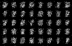
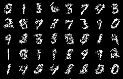
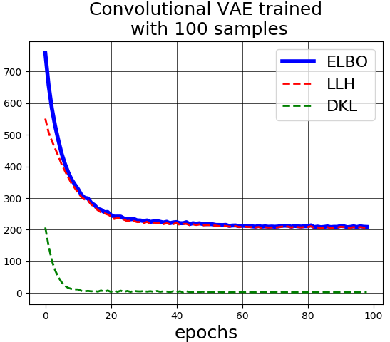
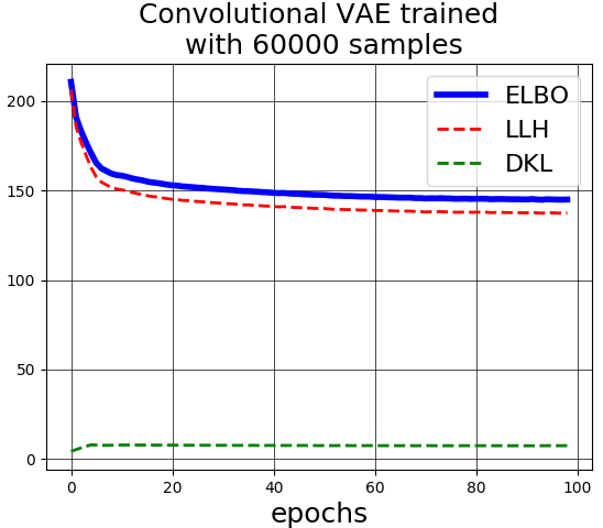
Figure 1: Samples obtained by decoding a sample from the prior distribution with two VAEs trained on 100 (top left) and 60000 (top right) samples from the MNIST database. Below we plot the reconstruction error (red dashed line) showing that although we are minimizing it, we cannot generate good quality images. Acronyms: $ELBO$ evidence lower bound; $D_{KL}$ Kullback-Lieber divergence and $LLH$ log-likelihood.

In this work we study how we can apply deep learning techniques when the amount of data is very scarce. We simulate scenarios where not only the amount of labeled data is scarce, but all the available data. As mentioned before, some techniques can deal with such scenarios. Bayesian modeling incorporates the uncertainty in the model [3]. However Bayesian neural networks are a field under study and introduce several problems for which there is not a wide well established solution: Monte Carlo integration, variational approximations or sampling in high dimensional data spaces, among others.

On the other hand, semi supervised learning techniques need a great amount of unlabeled data to work well. For instance, the ladder network can achieve impressive results with only 100 labeled samples in the MNIST task but using 60000 unlabeled samples.

Finally, deep generative models (DGM) need great amounts of data to be able of generate good quality samples. Figure 1 shows a Variational Auto-encoder (VAE) trained with 100 and 60000 samples. We can see that although the reconstruction error is being minimized the VAE with few samples is unable to generate good samples.

To our knowledge, none of the above mentioned techniques (both semi supervised and DA with DGM) has been applied disruptively to train neural networks models in data scarce scenarios as the ones we propose. Moreover DA based on DGM has not achieved impressive results in neural networks training with lots of data.

In this work we show that simple generative models as the Restricted Boltzmann Machines (RBM) [1] clearly outperforms the ladder network and DA based on a Deep Convolutional Variational Auto-encoder.

2 Methodology

In this work we simulate very scarce data scenarios. We train binary VAE and RBM using all the available samples. Details on these models can be found at [1, 9, 14]. Once these models are trained, we perform a sample generation following a MCMC procedure.

2.1 Sample Generation

For sample generation we rely on the theory of MCMC algorithms and define our transition operator as:

$$\mathcal{T}(x^{\prime}|x)=\int dh\,p(x^{\prime}|h)\cdot p(h|x)$$ (1)

Where $p(x^{\prime}|h)$ and $p(h|x)$ represents the likelihood distribution of an observed sample $x$ given a latent variable $h$ and, the posterior distribution over the latent variable given an observed sample, respectively. We will assume that this transition operator generates an ergodic Markov Chain and thus as long as the number of generated samples goes to infinity we will be sampling from the model distribution $p(x)$ [11, 3, 2]. In case of VAEs, where the posterior distribution is approximated, see [14] appendix F for a proof of correctness.

In our models the likelihood distribution $p(x|h)$ is modeled with a Bernoulli distribution. The posterior distribution is modeled with a Bernoulli distribution for the RBM and with a factorized Gaussian distribution for the VAE. For generating a sample we follow the Contrastive Divergence [4] algorithm which is based on Gibbs Sampling but starting from an observed sample. As example for generating 100 samples we follow algorithm 1, where $x$ is a sample from our dataset from which we will be generating new samples and $N$ is the number of samples to generate.

Input: $x$ , $N$

Output: generated_chain

generated_chain=vector($N$)

$x^{\prime}=x$

for $i=0$ until $N-1$  do

       $h^{\prime}\sim p(h|x^{\prime})$

       $x^{\prime}\sim p(x|h^{\prime})$

       generated_chain[$i$]$=x^{\prime}$

end for

Algorithm 1 Running MCMC algorithm for data generation

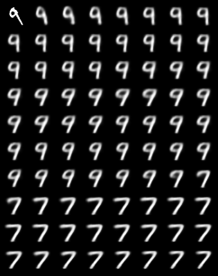
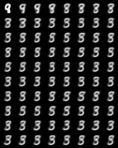
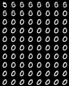
Figure 2: This figure shows $\mathbb{E}_{x\sim p(x|h)}\{x\}$ of a Markov Chain run with a VAE trained on 60000 samples, starting from a test image (image on the top left corner). We can clearly see how the generated samples can change from class as we run the algorithm. Image in the middle starts from an 8, then, the two next generated samples are 9s to after generate 8s and finally generate 3s. Sample on the right starts from a 5, generate some 5s and finally generate 0s.

2.2 Labeling process

We use the generated samples in two ways. As we stated, our approach is based on training a classifier on a set of labeled samples using additional generated samples from a VAE or a RBM. We associate the generated samples with the same label as the sample from the data distribution. In a first approach we use all the generated samples (and denote this approach in the experiments with letter $n$). In the second approach we classify the samples from the chain (using the same classifier we are training) and only the correctly classified samples are used for training (we denote this approach in the experiments with letter $y$). This has a great impact, as shown in the experiments, because long Markov Chains are likely to generate samples from other classes, as shown in figure 2.

Moreover, in case of the RBM we train two kind of models, named B-RBM (”bad RBM”) and G-RBM (”good RBM”). The difference rely on the convergence of the model, i.e., how is the quality of the generated samples, see figure 3. We expect that with a B-RBM the injected noise is able to improve the generalization whereas the G-RBM is collapsing to a part of the model space where no generalization improvement will be obtained. Basically we do not let the model achieve the same minimum for the case of the B-RBM as we do with the G-RBM.

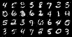
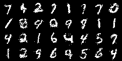
Figure 3: Samples from a bad (left) and good (right) RBM. Figure shows a sample from a MCMC chain of 1 step starting from a test sample.

Finally, figure 4 shows images from the different trained models in this work. We can clearly see how the VAE is able to generate good quality samples only when more training samples are provided.

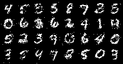
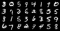
(a) B-RBM trained with 100 samples (left) and 1000 samples (right).

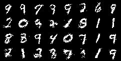
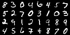
(b) G-RBM trained with 100 samples (left) and 1000 samples (right).

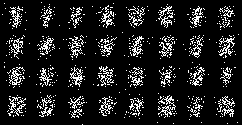
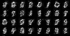
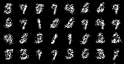
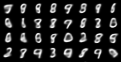
(c) Samples from a VAE trained with 100 samples (left), 1000 samples (middle left), 10000 samples (middle right) and $\mathbb{E}_{x\sim p(x|h)}\{x\}$ on 10000 samples (right)

Figure 4: Samples from our proposed generative models

3 Experiments

For the experiments we use a binarized version from the MNIST database. This database has 60000 training samples and 10000 test samples. The pixels above $0.5$ are saturated to value $1.0$ and the rest are saturated to $0.0$. In order to simulate a scarce data scenario, we randomly select a small set of samples, and assume that only a very small subset is labeled. We simulate three different scenarios with a total of $100$, $1000$ and $10000$ samples where only $10$, $100$ and $1000$ are labeled respectively. Note that for the first scenario we have only $1$ labeled sample per class.

We use a binarized version of this database because, the expressions of the conditional distributions of the RBM models we use, are obtained assuming binary data distributions. Moreover, the VAE models for MNIST converge better when using Bernoulli decoders , ie binary cross entropy loss.

We trained 3 models, two fully connected (FC) and one convolutional (CNN). For fully connected we choose the following parameters, FC1: 784-1024-1024-10, FC2: 784-1000-500-250-250-250-10. For the convolutional counterpart we use, CONV1: 32@3x3-64@3x3-128@3x3-512-512-10. In all the topologies we inject Gaussian noise with $\sigma=0.3$ in the input and we use batch norm (BN)[8] and dropout [15])

Tables 1, 2 and 3 show the error percentage with the here proposed data augmentation showing that the B-RBM clearly outperforms other approaches. We generate Markov chains of 500 and 1000 samples to increase the data set and train the classifier. It is interesting to see that although the deep FC (FC2) has worse performance than FC1 with 10 and 100 samples without DA, we can achieve better results in case of 100 samples with FC2 when using our proposed method.

We also see that a significant improvement is obtained with the most scarce scenario (see table 1), where we are able to reduce 17% error on CONV1 (check B-RBM option $y$ 1000 samples) and more than 10% in FC models (check B-RBM option $y$), which is the main objective of this work.

Table 1: Data Augmentation for 10 labeled samples

Baseline B-RBM G-RBM VAE Chain Length 500 1000 500 1000 500 1000 Classify y n y n y n y n y n y n FC1 53.71 44.71 47.87 43.19 47.56 53.49 52.55 53.91 52.5 80.25 51.49 84.48 50.56 FC2 58.88 45.34 47.18 46.4 46.26 54.74 55.27 57.43 57.96 78.14 56.91 78.79 56.66 CONV1 49.58 33.77 37.51 32.26 36.69 41.260 38.94 40.12 40.66 39.35 41.56 44.86 41.47

Table 2: Data Augmentation for 100 labeled samples

Baseline B-RBM G-RBM VAE Chain Length 500 1000 500 1000 500 1000 Classify y n y n y n y n y n y n FC1 26.56 21.34 21.61 21.41 22.43 26.83 26.51 28.41 26.86 52.01 37.00 - - FC2 28.39 19.72 21.31 18.66 22.31 26.95 26.98 25.96 26.54 64.82 43.99 - - CONV1 12.41 11.65 13.55 - - 11.36 11.25 - - 58.35 30.14 - -

Table 3: Data Augmentation for 1000 labeled samples

Baseline B-RBM G-RBM VAE Chain Length 500 1000 500 1000 500 1000 Classify y n y n y n y n y n y n FC1 7.62 5.55 6.16 5.81 6.04 5.86 5.91 5.79 5.97 24.13 12.42 - - FC2 7.25 5.60 5.96 5.76 5.62 5.28 5.40 4.70 5.49 36.19 18.00 - - CONV1 3.11 3.26 3.89 - - 3.09 3.54 - - 10.19 4.85 - -

Finally, Table 4 shows a comparison with the ladder network. Ladder network can be considered the state-of-the art on semi-supervised learning on this dataset. As can be seen we obtain better results on the three scenarios.

Table 4: A comparison with the ladder network. We represent error percentage.

Labeled Samples	10	100	1000
Baseline	58.88	28.39	7.25
Ladder Network	48.85	24.74	6.96
RBM DA	45.34	18.66	5.60

4 Conclusions

We can draw several conclusions from this work. We first show that in data scarcity scenarios simple generative models outperform deep generative models (like VAEs). We also see that a B-RBM is incorporating noise that is improving generalization. We can check that G-RBM and VAE works better when we do not classify the generated sample and this is in fact another way to incorporate noise into the classifier. However B-RBM is the best of the three. This also means that a generative model trained in this way (where latent variables capture high detail) is unable to generate samples that improve generalization. The G-RBM generates better quality images but is unable to improve classification accuracy as the B-RBM does.

This can also be noted when we add more training samples, where the difference between the baseline and the here proposed DA is lower, as with CNN. This is because the samples generated do not incorporate additional information to the model and are either quite similar between them or quite similar to the labeled samples. A possible hypothesis is that the generative model is collapsing to a part of the data feature space.

VAEs results were unexpected because despite the poor quality images generated it can improve performance over the baseline. We got this improvement always without classifying images, model $n$, and only in the case where few label samples are used. It is clear that the VAE is not a good model for these scenarios.

Finally, we also show that the here proposed approach outperforms and is clearly an alternative to semi supervised learning in data scarcity scenarios as shown in table 4. Another important advantage is that RBM is robust and has a stable learning whether the ladder network and GAN frameworks have several training challenges. The ladder network has many hyper-parameters and its performance is really sensible to little changes on them and the GANs are quite sensible to hyper-parameters as well.

5 Acknowledgment

We gratefully acknowledge the support of NVIDIA Corporation with the donation of two Titan Xp GPU used for this research. The work of Daniel Ramos has been supported by the Spanish Ministry of Education by project TEC2015-68172-C2-1-P. Juan Maroñas is supported by grant FPI-UPV.

References

- [1] Y. Bengio. Learning deep architectures for ai. Found. Trends Mach. Learn., 2(1):1–127, Jan. 2009.
- [2] Y. Bengio et al. Generalized denoising auto-encoders as generative models. In Advances in Neural Information Processing Systems 26, pages 899–907. Curran Associates, Inc., 2013.
- [3] C. M. Bishop. Pattern Recognition and Machine Learning. Springer-Verlag, 2006.
- [4] Carreira-Perpinan et al. On contrastive divergence learning. In Aistats, volume 10, pages 33–40. Citeseer, 2005.
- [5] Y. Gal and Z. Ghahramani. Bayesian convolutional neural networks with Bernoulli approximate variational inference. In 4th International Conference on Learning Representations (ICLR) workshop track, 2016.
- [6] I. Goodfellow et al. Generative adversarial nets. In Advances in Neural Information Processing Systems 27, pages 2672–2680. Curran Associates, Inc., 2014.
- [7] G. Hinton et al. Deep neural networks for acoustic modeling in speech recognition. IEEE Signal Processing Magazine, 29:82–97, 2012.
- [8] S. Ioffe et al. Batch normalization: Accelerating deep network training by reducing internal covariate shift. In Proceedings of the 32Nd International Conference on International Conference on Machine Learning - Volume 37, ICML’15, pages 448–456. JMLR.org, 2015.
- [9] D. P. Kingma et al. Auto-encoding variational bayes, 2013.
- [10] T. Mikolov et al. Efficient estimation of word representations in vector space. 2013.
- [11] R. M. Neal. Probabilistic inference using markov chain monte carlo methods. 1993.
- [12] A. Rasmus et al. Semi-supervised learning with ladder networks. In Advances in Neural Information Processing Systems 28, pages 3546–3554. Curran Associates, Inc., 2015.
- [13] J. Redmon et al. You only look once: Unified, real-time object detection. In 2016 IEEE Conference on Computer Vision and Pattern Recognition, CVPR 2016, Las Vegas, NV, USA, June 27-30, 2016, pages 779–788, 2016.
- [14] D. J. Rezende et al. Stochastic backpropagation and approximate inference in deep generative models. In Proceedings of the 31st International Conference on International Conference on Machine Learning - Volume 32, ICML’14, pages II–1278–II–1286. JMLR.org, 2014.
- [15] N. Srivastava et al. Dropout: A simple way to prevent neural networks from overfitting. Journal of Machine Learning Research, 15:1929–1958, 2014.
- [16] I. Sutskever et al. Sequence to sequence learning with neural networks. In Advances in Neural Information Processing Systems 27, pages 3104–3112. Curran Associates, Inc., 2014.
- [17] C. Szegedy et al. Inception-v4, inception-resnet and the impact of residual connections on learning. 2016.
- [18] Tran et al. A bayesian data augmentation approach for learning deep models. In I. Guyon et al., editors, Advances in Neural Information Processing Systems 30, pages 2797–2806. Curran Associates, Inc., 2017.
- [19] A. van den Oord et al. Conditional image generation with pixelcnn decoders. In Advances in Neural Information Processing Systems 29, pages 4790–4798. Curran Associates, Inc., 2016.