Eigenvector Models for Solving the Seismic Inverse Problem for the Helmholtz Equation: Extended Materials

Abstract

We study the seismic inverse problem for the recovery of subsurface properties in acoustic media. In order to reduce the ill-posedness of the problem, the heterogeneous wave speed parameter is represented using a limited number of coefficients associated with a basis of eigenvectors of a diffusion equation, following the regularization by discretization approach. We compare several choices for the diffusion coefficient in the partial differential equations, which are extracted from the field of image processing. We first investigate their efficiency for image decomposition (accuracy of the representation with respect to the number of variables and denoising). Next, we implement the method in the quantitative reconstruction procedure for seismic imaging, following the Full Waveform Inversion method, where the difficulty resides in that the basis is defined from an initial model where none of the actual structures is known. In particular, we demonstrate that the method is efficient for the challenging reconstruction of media with salt-domes. We employ the method in two and three-dimensional experiments, and show that the eigenvector representation compensates for the lack of low-frequency information, it eventually serves us to extract guidelines for the implementation of the method.

1 Introduction

We consider the inverse problem associated with the propagation of time-harmonic waves which occurs, for example, in seismic applications, where the mechanical waves are used to probe the Earth. Following the non-intrusive geophysical setup for exploration, we work with measured seismograms that record the waves at the surface (i.e., partial boundary measurements) and one-side illumination (back-scattered/reflection data). In the last decades, this problem has encountered a growing interest with the increase in numerical capability and the use of supercomputers. However, the accurate recovery of the deep subsurface structures remains a challenge, due to the nonlinearity and ill-posedeness of the problem, the availability of partial reflection data only, and the large scale domains of investigation.

In the context of seismic, the quantitative reconstruction of physical properties using an iterative minimization of a cost function originally follows the work of Bamberger et al. (1979), Lailly (1983) and Tarantola (1984, 1987) in the time-domain, Pratt et al. (1990; 1996; 1998) for the frequency approach. The method is commonly referred to as Full Waveform Inversion (FWI), which takes the complete observed seismograms for data. One key of FWI is that the gradient of the misfit functional is computed using the adjoint-state method (Lions & Mitter, 1971; Chavent, 1974), to avoid the formation of the (large) Jacobian matrix; we refer to Plessix (2006) for a review in geophysical applications. Then, Newton-type algorithms represent the traditional framework to perform the iterative minimization. Due to the large computational scale of the domain investigated, seismic experiments may have difficulties to incorporate second order (Hessian) information in the algorithm, and alternative techniques have been proposed, for example, in the work of Pratt et al. (1998); Akcelik et al. (2002); Choi et al. (2008); Métivier et al. (2013); Jun et al. (2015). The quantitative (as opposed to qualitative) reconstruction methods based upon iterative minimization are naturally not restricted to seismic and we refer, among others, to Ammari et al. (2015); Barucq et al. (2018) and the references therein for additional applications using similar techniques.

The main difficulty of FWI (in both exploration and global seismology) lies in the high nonlinearity of the problem and the presence of local minima in the misfit functional, which are due to the time shifts and cycle-skipping effect (Bunks et al., 1995), in particular when the background velocity (the low-frequency profile) is not correctly anticipated (Gauthier et al., 1986; Luo & Schuster, 1991; Fichtner et al., 2008; Barucq et al., 2019b). For this reason, the phase information is included in the traveltime inversion by Luo & Schuster (1991) by using a cross-correlation function between measurements and simulations, where the relative phase shift is given by the maximum of the correlation. The method is further generalized by Gee & Jordan (1992), while Van Leeuwen & Mulder (2010) propose to select the phase shift using a weighted norm. The choice of misfit has further encountered a growing interest in the past decade: in application to global-scale seismology, Fichtner et al. (2008) compare the phase, correlation-based, and envelope misfit functionals, the latter being also studied by Bozdağ et al. (2011). In exploration seismic, comparisons of phase and amplitude inversion are performed by Bednar et al. (2007); Pyun et al. (2007). The $L1$ norm is studied by Brossier et al. (2010) while approaches based upon optimal transport are considered by Métivier et al. (2016); Yang et al. (2018). In the context where different fields are measured, Alessandrini et al. (2019); Faucher et al. (2019) advocate for a reciprocity-based functional, which further connects to the correlation-based formulas (Faucher et al., 2019). In the case of accurate knowledge of the background velocity, the inverse problem is close to linear or quasi-linear as the Born approximation holds and then, alternative methods of linear inverse problem can be applied, such as the Backus–Gilbert method (Backus & Gilbert, 1967, 1968). The difficulty to recover the background velocity variation has also motivated alternative parametrization of the inverse problem: for instance the MBTT (Background/Data-Space Reflectivity) reformulation of FWI (Clément et al., 2001; Barucq et al., 2019b).

In order to diminish the ill-posedness of the inverse problem, a regularization criterion can be incorporated. It introduces an additional constraint (in addition to the fidelity between observations and simulations), which, however, may be complicated to select a priori and problem dependent (with ‘tuning’ parameters). For instance, we refer to the body of work of Kirsch (1996); Isakov (2006); Kern (2016); Kaltenbacher (2018) and the references therein. In the regularization by discretization approach, the model representation plays the role of regularizing the functional, by controlling (and limiting) the number of unknowns in the problem, and possibly defining (i.e. constraining) the shape of the unknown (e.g., to force smoothness). Controlling the number of unknowns influences the resolution of the outcome, but also the stability and convergence of the procedure. The use of piecewise constant coefficients appears natural for numerical applications, and is also motivated by stability results (Alessandrini & Vessella, 2005; Beretta et al., 2016). However, such a decomposition can lead to an artificial ‘block’ representation (cf. Beretta et al. (2016); Faucher (2017)) which would not be appropriate in terms of resolution. For this reason, a piecewise linear model representation is explored by Alessandrini et al. (2018, 2019), still motivated by the stability properties. We also mention the wavelet-based model reductions, that offer a flexible framework and are used for the purpose of regularization in seismic tomography by Loris et al. (2007, 2010). In the work of Yuan et al. (2014; 2015), FWI is carried out in the time-domain with a model represented from a wavelet-based decomposition.

In our work, we will use a model decomposition based upon the eigenvectors of a chosen diffusion operator, as introduced by De Buhan & Kray (2013); Grote et al. (2017); Grote & Nahum (2019). Note that this decomposition is shown (with the right choice of operator) to be related with the more standard Total Variation (TV) or Tikhonov regularizations. The main difference in our work is that we study several alternatives for the choice of the operator following image processing techniques, which traditionally also relies on such diffusion PDEs (e.g. Weickert (1998)). We first investigate the performance of the decomposition depending on the choice of PDE, and, next, the performance of such a model decomposition as parametrization of the reconstruction procedure in seismic FWI. It shows that the efficient choice of PDE should change depending on the situation. In addition, we provide a series of experiment to extract the robust guidelines for the implementation of the method in seismic.

We specifically target the reconstruction of subsurface salt domes (i.e. media with high contrasting objects), which is particularly challenging, because (in addition to the usual restrictive data) of the change of the kinematics involved and the lack of low frequency data (Farmer et al., 1996; Chironi et al., 2006; Virieux & Operto, 2009; Barucq et al., 2019a). In such cases, the use of the Total-Variation regularization (Rudin et al., 1992) with FWI is becoming more and more prominent, and consists in incorporating an additional constraint on the model in the minimization problem. Its efficiency is shown in the context of acoustic media with salt-dome contrasts by, e.g., Brandsberg-Dahl et al. (2017); Esser et al. (2018); Kalita et al. (2019); Aghamiry et al. (2019). In our work, we study several alternatives and demonstrate that the model representation with the criterion extracted from Geman & Reynolds (1992) appears the most appropriate for the eigenvector decomposition method in the presence of salt-domes. We also show the limitations of the method, in particular, it appears that the decomposition fails to represent models which are composed of several thin structures.

In Section 2, we define the inverse problem associated with the Helmholtz equation and introduce the iterative method for the reconstruction of the wave speed. In Section 3, we review several possibilities for the model decomposition using the eigenvectors of the diffusion operators. The process of model (image) decomposition is illustrated in Section 4. Then, in Section 5, we carry out the iterative reconstruction with FWI experiments in two and three dimensions. Here, the model decomposition is based upon the initial model, which does not contain a priori information on the target, hence increasing the differences of performance depending on the selection of the basis. It allows us to identify the best candidate for the recovery of salt dome, and to extract some guidelines for applications in quantitative reconstruction.

2 Inverse time-harmonic wave problem

2.1 Forward problem

We consider a domain $\Omega$ in two or three dimensions, with $\Omega\subset\mathbb{R}^{2}$ or $\Omega\subset\mathbb{R}^{3}$. We focus on acoustic media where, for simplicity, the density is taken as a constant, leading us to the identification of a single heterogeneous parameter: the wave speed. The propagation of waves in an acoustic medium with constant density is given by the scalar pressure field $p$, solution to the Helmholtz equation

$$\Big{(}-\Delta-\omega^{2}c^{-2}(\boldsymbol{x})\Big{)}p(\boldsymbol{x})=f(\boldsymbol{x}),\quad\quad\text{in $\Omega$},$$ (1)

where $c$ is the wave speed, $f$ the source, and $\omega$ the angular frequency. We now have to specify the boundary conditions to formulate the appropriate problem.

Following a seismic setup, the boundary of $\Omega$, $\Gamma$ is separated into two. The upper (top) boundary, $\Gamma_{1}$, represents the interface between the Earth and the air, and is subsequently represented via a free surface boundary condition, where the pressure is null. On the other hand, other part of the boundary corresponds to the numerical need for restricting the area of interest. Here, conditions must ensure that entering waves are not reflected back to the domain (i.e., because the area of interest is only a part of the Earth), see Figure 1. The two most popular formulations to handle such numerical boundary are either the Perfectly Matched Layers (PML, Bérenger (1994)), or outgoing artificial boundary conditions. In our case, we use Absorbing Boundary Conditions (ABC, Engquist & Majda (1977)) so that the complete problem writes as

$$\left\{\begin{aligned} \big{(}-\Delta-\omega^{2}c^{-2}(\boldsymbol{x})\big{)}p(\boldsymbol{x})&=f(\boldsymbol{x}),\quad\quad&\text{in $\Omega$},\\ p(\boldsymbol{x})&=0,\quad\quad&\text{on $\Gamma_{1}$},\\ \partial_{\nu}p(\boldsymbol{x})-\mathrm{i}\omega c^{-1}(\boldsymbol{x})p(\boldsymbol{x})&=0,\quad\quad&\text{on $\Gamma_{2}$},\\ \end{aligned}\right.$$ (2)

where $\partial_{\nu}$ is the normal derivative. We recall that $p$ denotes the pressure, $\omega$ denotes the frequency of the induced source and $c$ denotes the wave speed.

The inverse problem aims the recovery of the wave speed $c$ in (2), from a discrete set of measurements (i.e. partial data), which corresponds to observation of the wave propagations. More precisely, our data consist in measurements of the pressure field solution to (2), at the (discrete) device locations. We refer to $\Sigma$ for this set of positions, where the receivers are located, and define the forward map at frequency $\omega$, $\mathcal{F}_{\omega}$ (which links the model to the data), such that,

$$\mathcal{F}_{\omega}~{}:~{}m\,\,\rightarrow\,\,p(\boldsymbol{x})\mid_{\Sigma}.$$ (3)

We have introduced $m(\boldsymbol{x}):=c^{-2}(\boldsymbol{x})$, which is also our choice of parameter for the reconstruction, see Remark 2. In seismic, the data are further generated from several point sources (excited one by one) and all devices (sources and receivers) remain near the surface. All devices (sources and receivers) remain near the surface ($\Gamma_{1}$), as illustrated with $\Sigma$ in Figure 1.

Figure 1: Illustration of the two-dimensional computational domain. The sign ‘plus’ indicates the (point) source and the dotted line is the location of the discrete measure points. The complete acquisition consists in several sources, all are located at the same depth, only the lateral position varies; the measure points are fixed.

2.2 Quantitative reconstruction using iterative minimization

The inverse problem aims the reconstruction of the unknown medium squared slowness $m$ (i.e. the wave speed) from data $\boldsymbol{y}_{\omega}$ that connects to the forward map $\mathcal{F}_{\omega}(m_{\dagger})$ for a reference (target) model $m_{\dagger}$ with

$$\boldsymbol{y}_{\omega}=\mathcal{F}_{\omega}(m_{\dagger})+\mathfrak{E}_{\omega},$$ (4)

where $\mathfrak{E}_{\omega}$ represents the noise in the measurements (from the inaccuracy of the devices, model error, etc), possibly frequency dependent.

For the reconstruction, we follow the Full Waveform Inversion (FWI) method (Tarantola, 1984; Pratt et al., 1998), which relies on an iterative minimization of a misfit functional defined as the difference between the observed data and the computational simulations:

$$\min_{m}\mathcal{J}(m)=\dfrac{1}{2}\sum_{\omega}\|\mathcal{F}_{\omega}(m)-\boldsymbol{y}_{\omega}\|^{2},$$ (5)

where we use the standard least-squares minimization but alternatives have also been studied, as indicated in the introduction.

Remark 1 (Multi-frequency algorithm).

For the choice of frequency in Problem 5, applications commonly use a sequence of increasing frequencies during the iterative process (Bunks et al., 1995; Pratt & Worthington, 1990; Sirgue & Pratt, 2004; Brossier et al., 2009; Barucq et al., 2018; Faucher, 2017). Namely, one starts with a low frequency and minimize the functional for the fixed frequency content in the data. Once the misfit functional stagnates, or after a prescribed number of iterations, the frequency is updated (increased) and the iterations continue, cf. Algorithm 2. Moreover, the use of sequential frequency (instead of band of frequencies) is advocated by Barucq et al. (2019a), because it enlarges the size of the basins of attraction.

Remark 2 (Parametrization of the unknown).

For the reconstruction, we invert the squared slowness $m=c^{-2}$ instead of the velocity. The choice of this parameter is first motivated by the Helmholtz equation (2). However, it (i.e., velocity, slowness or squared slowness inversion) can lead to an important difference in the efficiency of the reconstruction procedure. It is discussed, for example, by Tarantola (1986); Brossier (2011); Köhn et al. (2012); in particular, we motivate our choice from the comparison of reconstructions provided in the context of seismic by (Faucher, 2017, Section 5.4).

Then, an iterative minimization algorithm is used for the resolution of Problem 5 in the framework of the Newton methods. Starting with an initial guess $m^{(0)}$, the model is updated at each iteration $k$, using a search direction $s^{(k)}$, such that

$$m^{(k+1)}=m^{(k)}+\mu s^{(k)},\qquad k\,>\,0.$$ (6)

Several possibilities exist for the search direction (e.g., Newton, Gauss-Newton, BFGS, gradient descent, etc.) and we refer to Nocedal & Wright (2006) for an extensive review of the methods. The scalar coefficient $\mu$ is approximated using a line search algorithm (Nocedal & Wright, 2006). In our implementation, we rely on a gradient-based optimization, with the nonlinear conjugate gradient method, and a backtracking line search (Nocedal & Wright, 2006). A review of the performance of first order-based minimization algorithms and the influence of line search step selection is further investigated by Barucq et al. (2018) in the context of inverse scattering. The computation of the gradient of the misfit functional is carried out using the adjoint-state method (Chavent, 1974; Plessix, 2006), which specific steps for complex-valued fields can be found in (Barucq et al., 2019b, Appendix A)

3 Regularization by discretization: model decomposition

In this section, we introduce a representation of the unknown, i.e., the model decomposition, based upon the eigenvectors of a diffusion equation. The objective is to reduce the dimension of the unknown to mitigate the ill-posedness of the inverse problem. We provide several possibilities for the choice of the eigenvectors, following the literature in image processing.

3.1 Regularization and diffusion operators

The resolution of the inverse problem using a quantitative method introduces an optimization problem (5) where the misfit functional $\mathcal{J}$ accounts for a fidelity term. The resolution of such a problem is also common in the context of image processing (e.g., for denoising or edge enhancement) where the fidelity term corresponds to the matching between the original and processed images. It is relatively common (for both the quantitative reconstruction methods and in image processing) to incorporate an additional term in the minimization, for the purpose of regularization. The primary function of this additional term is to reduce the ill-posedness of the problem, by adding a constraint. It has been the topic of several studies, we refer to, e.g., Kirsch (1996); Isakov (2006); Charbonnier et al. (1994); Robert & Deriche (1996); Rudin et al. (1992); Vogel & Oman (1996); Lobel et al. (1997); Kern (2016); Qiu et al. (2016); Kaltenbacher (2018). The regularized minimization problem writes as

$$\min_{m}\mathcal{J}_{r}(m)=\dfrac{1}{2}\sum_{\omega}\|\mathcal{F}_{\omega}(m)-\boldsymbol{y}_{\omega}\|^{2}+\mathcal{I}(m),$$ (7)

where $\mathcal{I}$ stands for the regularization term.

In many applications such as image processing, $\mathcal{I}$ is usually defined to only depend on the gradient of the variable (image), such that

$$\mathcal{I}(m)=\int_{\Omega}\phi(|\nabla m|)\,\,\mathrm{d}\Omega\,,$$ (8)

where $\phi\in L^{2}(\Omega)$. In particular, the minimum of $\mathcal{I}$ with respect to $m$ verifies the Euler–Lagrange equations (Evans, 2010; Dubrovin et al., 1992). In one dimension, it is given by (Dubrovin et al., 1992, Theorem 31.1.2) and is extended for higher dimensions with (Dubrovin et al., 1992, Theorem 37.1.2) (further simplified in our case because $\mathcal{I}$ only depends on the gradient). It states that the minimizer of $\mathcal{I}$ is the solution of the diffusion equation:

$$\nabla\cdot\bigg{(}\dfrac{\phi^{\prime}(|\nabla m|)}{|\nabla m|}\nabla m\bigg{)}=0\quad\quad\text{in $\Omega$.}$$ (9)

For the sake of clarity, we introduce the following notation:

$$\mathcal{A}(\mathrm{y},\,\eta):=-\nabla\cdot\big{(}\eta(\mathrm{y})\nabla\big{)},\quad\quad\quad\text{with}\quad\quad\eta(\mathrm{y})=\dfrac{\phi^{\prime}(|\nabla\mathrm{y}|)}{|\nabla\mathrm{y}|}.$$ (10)

In the following, we present several choices for the diffusion PDE coefficient $\eta$, following image processing theory.

Remark 3.

The minimization of $\mathcal{J}_{r}$ in Problem (7) can be performed using traditional gradient descent or Newton type algorithms. Another alternative, in particular when rewriting with the Euler–Lagrange formulation in the context of image processing, is to recast the problem as a time dependent evolution one, see, e.g., the work of Weickert (1998); Catté et al. (1992); Rudin et al. (1992); Alvarez et al. (1992).

Remark 4.

The diffusion equation (9) is obtained using the fact that $\phi=\phi(|\nabla m|)$ only depends on $\nabla m$. In case of dependency of the function with $m$, or higher order derivatives, the Euler–Lagrange formulation must be adapted.

3.2 Diffusion coefficients from image processing

There exist several possibilities for the choice of diffusion coefficient $\eta$ (also referred to as the weighting function) in (10), inherited from image processing theory and applications. In the following, we investigate the most common formulations, see Table 1, for which we have mainly followed the ones that are reviewed by (Blanc-Féraud et al., 1995, Table 1) and Robert & Deriche (1996). Furthermore, we incorporate a scaling coefficient $\beta>0$ for the diffusion coefficient, which impacts on the magnitude. For consistency in the different models, the norms that we employed are scaled with the maximal values so that they remain between $0$ and $1$. We define,

$$g_{{1}}(m,\boldsymbol{x})=\dfrac{|\nabla m(\boldsymbol{x})|}{\gamma_{1}},\qquad g_{{2}}(m,\boldsymbol{x})=\dfrac{|\nabla m(\boldsymbol{x})|^{2}}{\gamma_{2}},\qquad\text{with}$$ (11)

$$\gamma_{1}=\max\big{(}|\nabla m(\boldsymbol{x})|\big{)}\,,\quad\gamma_{2}=\max\big{(}|\nabla m(\boldsymbol{x})|^{2}\big{)}\,,\quad|\nabla m(\boldsymbol{x})|=\sqrt{\sum_{k=1}^{\mathfrak{d}}\bigg{(}\dfrac{\partial m}{\partial x_{k}}\bigg{)}^{2}},$$

where $\mathfrak{d}$ is the space dimension ($\mathfrak{d}=2$ or $\mathfrak{d}=3$ in our experiments) and $\boldsymbol{x}$ the space coordinates: $\boldsymbol{x}=\{x_{k}\}_{k=1}^{\mathfrak{d}}$. In order to simplify the formulas, we will omit the space dependency in the following. Note that in the numerical experiments, we calculate the eigenvalues and eigenvectors from the linear differential operator $\mathcal{A}(m,\eta)$ defined in (10), where the diffusion coefficient $\eta$ is taken from the nonlinear PDE model.

Remark 5.

We can make the following comments regarding the nine diffusion coefficients that are introduced in Table 1.

• The PDE (9) using the Tikhonov diffusion coefficient $\eta_{9}$ coincides with the Laplace equation.

• For the formulation of $\eta_{4}$ and $\eta_{8}$, we have to impose a threshold as the coefficient is not defined for the points where the gradient is zero. In the computations, we impose that $\eta_{4}=\eta_{8}=1$ for the points $\boldsymbol{x}_{i}$ where $\nabla m(\boldsymbol{x}_{i})<\text{$10^{-12}$}$.

• The first Perona–Malik formula $\eta_{1}$, is very similar to the Lorentzian approach, $\eta_{6}$: only the position of $\beta$ differs. Namely, the Perona–Malik formula would rather use small $\beta$ while the Lorentzian formula would use large $\beta$.

• The second Perona–Malik formula, $\eta_{2}$, is very similar to the Gaussian criterion $\eta_{7}$, which only includes an additional dependency on $\beta$.

• The formulation of $\eta_{8}$ corresponds to the Total Variation (TV) regularization (Vogel & Oman, 1996).

Table 1: List of formula for the coefficient of the diffusion operator which is used to decompose the image.

reference (name)	definition	$\beta\rightarrow 0$	$\beta\rightarrow\infty$
Perona & Malik (1988, 1990)	$\eta_{1}(m,\beta)=\dfrac{\beta}{\beta+g_{{2}}(m)}$	0	1
Perona & Malik (1988, 1990)	$\eta_{2}(m,\beta)=\exp\bigg{(}-\dfrac{g_{{2}}(m)}{\beta}\bigg{)}$	0	1
Geman & Reynolds (1992)	$\eta_{3}(m,\beta)=\dfrac{2\beta}{\big{(}\beta+g_{{2}}(m)\big{)}^{2}}$	0	0
Green (1990)	$\eta_{4}(m,\beta)=\tanh\bigg{(}\dfrac{g_{{1}}(m)}{\beta}\bigg{)}\bigg{(}\dfrac{1}{\beta g_{{1}}(m)}\bigg{)}$	$+\infty$	0
Charbonnier et al. (1994)	$\eta_{5}(m,\beta)=\dfrac{1}{\beta}\bigg{(}\dfrac{\beta+g_{{2}}(m)}{\beta}\bigg{)}^{-1/2}$	$+\infty$	0
Grote & Nahum (2019)
(Lorentzian)	$\eta_{6}(m,\beta)=\dfrac{\beta}{\big{(}1+\beta g_{{2}}(m)\big{)}^{2}}$	0	0
Grote & Nahum (2019)
(Gaussian)	$\eta_{7}(m,\beta)=\bigg{(}\beta\exp\bigg{(}\dfrac{g_{{2}}(m)}{\beta}\bigg{)}\bigg{)}^{-1}$	0	0
Rudin et al. (1992)
(Total Variation, TV)	$\eta_{8}(m)=\dfrac{1}{g_{{1}}(m)}$	n/a	n/a
Tikhonov	$\eta_{9}=1$ $\dfrac{1}{2}$	n/a	n/a

3.3 Eigenvector model decomposition in FWI

In our work, we employ the regularization by discretization approach: instead of adding the regularization term $\mathcal{I}$ in the minimization problem, we remain with Problem (5), and use a specific representation for the model (unknown). We follow the work of De Buhan & Osses (2010); De Buhan & Kray (2013); Grote et al. (2017); Grote & Nahum (2019) with the “Adaptive Inversion” or “Adaptive Eigenspace Inversion” method. Namely, the unknown is represented via a decomposition into the basis of eigenvectors computed from a diffusion PDE. The purpose is to control the number of unknowns in the representation, and consequently reduce the ill-posedness of the inverse problem. The decomposition uses the steps (given in Grote et al. (2017)) depicted in Algorithm 1.

Eigenvector decomposition: given an initial model $m(\boldsymbol{x})$, a selected integer value $N>0$, and the selected diffusion coefficient $\eta$. 1. Compute $\mathfrak{m}_{0}$, the solution of the linear PDE $$\left\{\begin{aligned} \mathcal{A}(m,\eta)\mathfrak{m}_{0}&=0,\quad\quad&\text{in $\Omega$,}\\ \mathfrak{m}_{0}&=m,\quad\quad&\text{on $\Gamma$.}\end{aligned}\right.$$ (12) 2. Compute the subset of $N$ eigenfunctions $\{\psi_{k}\}_{k=1,\ldots,N}$ which are associated to the $N$ smallest eigenvalues $\{\lambda_{k}\}_{k=1,\ldots,N}$ such that, for all $k$, $$\left\{\begin{aligned} \mathcal{A}(m,\eta)\psi_{k}&=\lambda_{k}\psi_{k},\quad\quad&\text{in $\Omega$,}\\ \psi_{k}&=0,\quad\quad&\text{on $\Gamma$.}\end{aligned}\right.$$ (13) 3. Compute the model decomposition using $N$ eigenvectors: $$\mathfrak{m}=\mathfrak{m}_{0}+\sum_{k=1}^{N}\alpha_{k}\psi_{k},$$ (14) where $\alpha_{k}$ is a scalar and $\psi_{k}$ a vector. Here, the set of $\alpha$ is chosen to minimize $\|\mathfrak{m}-m\|^{2}$; and the $\psi_{k}$, $k=1,\ldots,N$ are the eigenvectors associated with the $N$ smallest eigenvalues $\lambda_{k}$, computed in Step (ii).

Algorithm 1 The model decomposition using the eigenvectors of the diffusion equation associated with the smallest eigenvalues. We refer to the model decomposition as ${\mathfrak{m}}(m,N,{\boldsymbol{\psi}})$ where ${\boldsymbol{\psi}}(m,\eta,N)$ is the set of eigenvectors, see (15) and (16).

Following Algorithm 1, we introduce the notation,

$${\boldsymbol{\psi}}(m,\eta,N)=\{\psi_{k}\}_{k=1,\ldots,N} N m$$ the set of eigenvectors associated with the model and (15)

th diffusion coefficient $$\eta$$, computed from (12) and (13);

and

$${\mathfrak{m}}(m,N,{\boldsymbol{\psi}})\qquad\text{is the decomposition of the model $m$ using $N$ vectors from ${\boldsymbol{\psi}}$,~{}\eqref{eq:methodEV_decomposition}.}$$ (16)

Therefore, the model is represented via $N$ coefficients $\alpha$ in (14) in the basis given by the diffusion operator. The reconstruction procedure follows an iterative minimization of (5), and performs successive update of the coefficients $\alpha$. The key is that $N$ is much smaller than the dimension of the original representation of $m$, but allows an accurate resolution, as we illustrate in Sections 4 and 5. Algorithm 2 details the procedure.

Inputs: the measurements $\boldsymbol{y}_{\omega}$; the initial model $m^{(0)}$; the selected number of iterations $n_{\text{iter}}$; the list of frequencies $\omega_{i}$, $i=1$,$\ldots$,$n_{\omega}$; the decomposition dimension associated with frequency: $N_{i}$, for $i=1,\ldots,n_{\omega}$. Using Algorithm 1, 1. compute the eigenvector basis for $m^{(0)}$ using the selected $\eta$ and the highest integer $N_{\max}=\max\big{(}\{N_{i}\}_{i=1}^{n_{\omega}}\big{)}$, $${\boldsymbol{\psi}}={\boldsymbol{\psi}}(m,\eta,N_{\max}).$$ (17) 2. Decompose the initial model using the initial decomposition dimension: $${\mathfrak{m}}^{(0)}={\mathfrak{m}}(m^{(0)},N_{1},{\boldsymbol{\psi}})=\mathfrak{m}_{0}+\sum_{l=1}^{N_{1}}\alpha_{l}^{(0)}\psi_{l}.$$ (18) Frequency loop for $i\in\{1,\ldots,n_{\omega}\}$ do

      

       Set $N=N_{i}$.

      Optimization loop for $j\in\{1,\ldots,n_{\text{iter}}\}$ do

            

Set $k:=(i-1)n_{\text{iter}}+j-1$.

Solve the Helmholtz equation (2) at frequency $\omega_{i}$ with model $\mathfrak{m}^{(k)}$.

Compute the misfit functional $\mathcal{J}$ in (5).

Compute the gradient of the misfit functional $\nabla_{\alpha}\mathcal{J}$ using the adjoint-state method.

Compute the search direction $s^{(k)}$, see Remark 6.

Compute the descent step $\mu$ using the line search algorithm, see Remark 6.

Update the coefficient $\alpha$ with $\alpha^{(k+1)}=\alpha^{(k)}-\mu s^{(k)}$.

Update the model:

$${\mathfrak{m}}^{(k+1)}={\mathfrak{m}}_{0}+\sum_{l=1}^{N}\alpha_{l}^{(k+1)}\psi_{l}.$$

       end for

      

end for

Algorithm 2 The iterative minimization algorithm (FWI) using the model decomposition to control the number of variables. The model is represented in the eigenvector basis, for which the weights are updated along with the iterations.

Remark 6 (Minimization algorithm).

For the minimization procedure depicted in Algorithm 2, we use a non-linear conjugate gradient method for the search direction. This method has the advantage that it only necessitates the computation of the gradient of the cost function (Nocedal & Wright, 2006). Then, to control the update step $\mu$ in Algorithm 2, a line search algorithm is typically employed (Eisenstat & Walker, 1994; Nocedal & Wright, 2006; Chavent et al., 2015; Barucq et al., 2018). This operation is complex in practice because an accurate estimation would require intensive computational operations (with an additional minimization problem to solve). Here, we employ a simple backtracking algorithm (Nocedal & Wright, 2006).

Remark 7 (Gradient computation).

The gradient of the cost function is computed using the first order adjoint-state method (Lions & Mitter, 1971; Chavent, 1974), which is standard in seismic application (Plessix, 2006). It avoids the formation of a dense Jacobian matrix and instead requires the resolution of an additional PDE, which is the adjoint of the forward PDE, with right-hand sides defined from the difference between the measurements and the simulations, see Plessix (2006); Faucher (2017); Barucq et al. (2018, 2019b) for more details.

In our implementation, the gradient is first computed with respect to the original (nodal) representation and we use the chain rule to retrieve the gradient with respect to the decomposition coefficients $\alpha$:

$$\dfrac{\partial\mathcal{J}}{\partial\alpha}=\dfrac{\partial\mathcal{J}}{\partial m}\dfrac{\partial m}{\partial\alpha}.$$ (19)

It is straightforward, from (14), that the derivation for a chosen coefficient ${\alpha_{l}}$ gives $\partial_{\alpha_{l}}m=\psi_{l}$. Therefore, it is computationally easy to introduce the formulation with respect to the eigenvector decomposition from an already existing ‘classical’ (i.e. when the derivative with respect to the model is performed) formulation: it only necessitates one additional step with the eigenvectors.

Remark 8.

In Algorithm 2, the basis of eigenvectors remains the same for the complete set of iterations, and is extracted from the initial model. Only the number of vectors taken for the representation, $N_{i}$, changes. Namely, from $N_{1}$ to $N_{2}>N_{1}$, the decomposition using $N_{2}$ still has the same $N_{1}$ first eigenvectors in its representation (with different weights $\alpha$), and additional $(N_{2}-N_{1})$ eigenvectors. As an alternative, we investigate the performance of an algorithm where the basis changes at each frequency (i.e. it is recomputed from the current iteration model), see Appendix A.

3.4 Numerical implementation

Our code is developed in Fortran90, it uses both mpi and OpenMP parallelism and run on cluster for efficiency. The forward wave operator is discretized using a Finite Differences scheme, e.g. Virieux (1984); Operto et al. (2009); Wang et al. (2011). The discretization of the Helmholtz operator generates a large sparse matrix, for which we use the direct solver Mumps (Amestoy et al. (2001, 2006)) for its factorization and the resolution of linear system. This solver is particularly optimized and designed for this type of linear algebra problems, i.e. large, sparse matrices. Our preference for direct solver instead of iterative ones is mainly motivated by two reasons:

1. seismic acquisition is composed of a large amount of sources, i.e. a large amount of right-hand sides (rhs) to be processed for the linear system. Using direct solver, the resolution time is very low once the factorization is performed, hence it is well adapted for the multi-rhs seismic configuration.

2. For the minimization algorithm, the gradient is computed via the adjoint-state method (see Remark 7). It means that an additional linear system has to be solved, which is actually the adjoint of the forward one. Here, the factors obtained from the factorization of the forward operator can be directly reused, and allow a reduced computational cost, see Barucq et al. (2018) and the references therein.

The next step is the computation of the eigenvectors associated with the smallest eigenvalues for the diffusion operator. We use the package Arpack, which is devoted to solve large sparse eigenvalue problems using iterative methods. More precisely, it uses implicitly restarted Lanczos or Arnoldi methods, respectively for symmetric and non-symmetric matrices, Lehoucq & Sorensen (1996). Several options are available in the package, including the maximum number of iterations allowed, or a tolerance parameter for the accuracy of acceptable solution.

Remark 9 (Eigenvectors associated with the lowest eigenvalues).

The Lanczos and Arnoldi methods are particularly efficient to compute the largest eigenvalues and associated eigenvectors of the matrix, and only require matrix vector multiplication. However, we are interested in the lowest eigenvalues for our decomposition. The idea is simply to use that the lowest eigenvalues of the discretized diffusion matrix, say $A$, are simply the largest eigenvalues of the matrix $A^{-1}$. Then, the matrix-vector multiplication, say $Av$ for a vector $v$, becomes a resolution of a linear system $A^{-1}v$. It may appear computationally expensive but it is not thanks to the use of the direct solver Mumps (see above), which, once the factorization is obtained, is very efficient for the resolution procedure. Hence, the computation follows the steps:

1. compute the (sparse) matrix discretization of the selected diffusion operator: $A$;

2. compute the factorization of the matrix $A$ using Mumps,

3. use the package Arpack to compute the largest eigenvalues of $A^{-1}$, by replacing the matrix-vector multiplication step in the iterations by the resolution of a linear system using Mumps.

Finally, the last step is to retrieve the appropriate coefficients $\alpha_{k}$ in (14) for the decomposition. It basically consists in the resolution of a dense linear system (from least squares method). We use Lapack, Anderson et al. (1999) (contrary to Mumps, Lapack is adapted to dense linear system). Note that, because we usually consider a few hundreds of coefficients for the decomposition, this operation remains relatively cheap compared to the eigenvectors computation. We compare the computational time for the eigenvectors computation and model decomposition in Figure 2 for different values of $N$ and $\eta$. We first note that the choice of $\eta$ does not really modify the computational time. Then, we see that the two operations are mostly linear in $N$, and that the time to solve the least squares problem with Lapack is much smaller than the time to compute the eigenvectors with Arpack, namely, hundred time smaller. For the largest case: $N=1000$ for a squared matrix of size 277221, it takes about 30min to retrieve the eigenvectors, and $10$ s to compute the $\alpha$ (in our applications we usually take $N<100$).

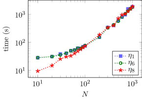
(a) The computational time to retrieve the eigenvectors associated with the lowest eigenvalues, (13), using sequential Arpack.

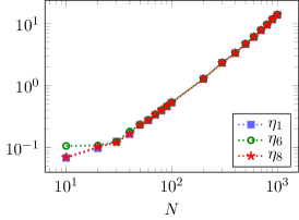
(b) The computational time to obtain the coefficients $\alpha$ in (14) using least squares method and sequential Lapack.

Figure 2: Comparison of the computational time for the eigenvector decomposition for different $\eta$. The computation of the eigenvectors uses the discretized matrix of a diffusion operator of size $\text{277221}\times\text{277221}$. It corresponds with the decomposition of the model Figure 3(b) which is further illustrated in Section 4. Other formulations of $\eta$ from Table 1 are not shown for clarity, but follow the exact same pattern.

4 Illustration of model decomposition

First, we illustrate the eigenvector model decomposition with geophysical media in two dimensions. The original model is represented on a structured grid by $n_{x}\times n_{z}$ coefficients, and we have here $921\times 301=\text{277221}$ coefficients. We consider three media of different nature:

• the Marmousi velocity model, which consists in structures and faults, see Figure 3(a);

• a model encompassing salt domes: objects of high contrast velocity, see Figure 3(b);

• eventually, the SEAM Phase I velocity model which consists in both salt and layer structures, see Figure 10.

All three models uses the same number of coefficients for their representations, and the first two are actually of the same size ($9.2\times 3$ km).

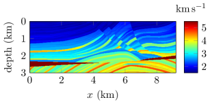
(a) Marmousi velocity model.

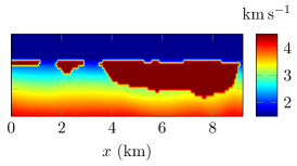
(b) Salt velocity model.

Figure 3: Seismic velocity models used to illustrate the eigenvector decomposition. They are both of size $9.2\times 3$ km and represented with $921\times 301$ nodal coefficients.

We perform the decomposition of the models by application of Algorithm 1, and steps (12), (13) and (14) (and we recall that we use the linear PDE problem). We study the main parameters of the decomposition:

• the choice of $\eta$, with the possibilities given in Table 1,

• the choice of the scaling parameter $\beta$ in the formulation of $\eta$ (Table 1),

• the number of eigenvectors $N$ employed for the decomposition in (14).

The accuracy of the decomposition is estimated using the $L^{2}$ norm of the relative difference between the decomposition and the original representation such that

$$\mathcal{E}=100\dfrac{\|m-\mathfrak{m}\|}{\|m\|},\quad\quad\text{Relative Error (\%)},$$ (20)

where $m$ is the original model (Figure 3) and $\mathfrak{m}$ the decomposition using the basis of eigenvectors from Algorithm 1.

4.1 Decomposition of noise-free models

We decompose the salt and Marmousi models using the nine possibilities for $\eta$, that are given in Table 1. For the choice of scaling coefficient $\beta$ (which does not affect $\eta_{8}$ and $\eta_{9}$), we roughly cover an interval from $10^{-7}$ up to $10^{6}$, namely: $\{$$10^{-7}$, $10^{-6}$, $10^{-5}$, $10^{-4}$, $10^{-3}$, $10^{-2}$, 5$.10^{-2}$, $10^{-1}$, 5$.10^{-1}$, 1, 5, 10, $10^{2}$, $10^{3}$, $10^{4}$, $10^{5}$, $10^{6}$$\}$. In Tables 2 and 3, we show the best relative error (i.e. minimal value) obtained for the Marmousi model of Figure 3(a) and the salt model of Figure 3(b). We test all choices of $\eta$ and values of $N$ between $10$ (coarse) and $500$ (refined). The corresponding values of the scaling parameter $\beta$ which gives the best (i.e. the minimal) error are also given in parenthesis.

Table 2: Minimal relative error obtained and associated scaling coefficient: $\mathcal{E}$ ($\beta$), for the decomposition of the Marmousi model Figure 3(a). The definition of $\eta$ is given Table 1.

Coeff.	$N=10$	$N=20$	$N=50$	$N=100$	$N=250$	$N=500$
$\eta_{1}$	6% ($10^{-6}$)	5% ($10^{-6}$)	4% ($10^{-6}$)	4% ($10^{-6}$)	3% ($10^{-6}$)	3% ($10^{-7}$)
$\eta_{2}$	14% (5.$10^{-2}$)	13% (5.$10^{-2}$)	12% (5.$10^{-2}$)	9% ($10^{-2}$)	7% ($10^{-2}$)	5% ($10^{-2}$)
$\eta_{3}$	8% ($10^{-4}$)	7% ($10^{-3}$)	6% ($10^{-3}$)	5% ($10^{-3}$)	5% ($10^{-3}$)	4% ($10^{-2}$)
$\eta_{4}$	14% (5.$10^{-1}$)	14% ($10^{1}$)	13% ($10^{1}$)	13% ($10^{-1}$)	12% (5.$10^{-1}$)	10% (5.$10^{1}$)
$\eta_{5}$	13% ($10^{-7}$)	12% ($10^{-6}$)	12% ($10^{-5}$)	10% ($10^{-5}$)	10% ($10^{-5}$)	6% ($10^{-7}$)
$\eta_{6}$	8% (5.$10^{3}$)	7% ($10^{3}$)	6% (5.$10^{2}$)	5% ($10^{3}$)	5% ($10^{3}$)	4% ($10^{2}$)
$\eta_{7}$	14% (5.$10^{-2}$)	13% (5.$10^{-2}$)	12% (5.$10^{-2}$)	11% (5.$10^{-2}$)	9% (5.$10^{-2}$)	7% (5.$10^{-2}$)
$\eta_{8}$	15% (n/a)	14% (n/a)	13% (n/a)	12% (n/a)	10% (n/a)	9% (n/a)
$\eta_{9}$	14% (n/a)	14% (n/a)	14% (n/a)	13% (n/a)	12% (n/a)	11% (n/a)

Table 3: Minimal relative error obtained and associated scaling coefficient: $\mathcal{E}$ ($\beta$), for the decomposition of the salt model Figure 3(b). The definition of $\eta$ is given Table 1.

Coeff.	$N=10$	$N=20$	$N=50$	$N=100$	$N=250$	$N=500$
$\eta_{1}$	4% ($10^{-3}$)	4% ($10^{-3}$)	3% ($10^{-2}$)	2% ($10^{-2}$)	1% ($10^{-2}$)	1% ($10^{-2}$)
$\eta_{2}$	9% ($10^{-1}$)	7% ($10^{-1}$)	5% ($10^{-1}$)	5% ($10^{-1}$)	4% ($10^{-1}$)	3% ($10^{-1}$)
$\eta_{3}$	8% (5.$10^{-2}$)	4%(5.$10^{-2}$)	3% (5.$10^{-2}$)	3% (5.$10^{-2}$)	2% (5.$10^{-2}$)	1% (5.$10^{-2}$)
$\eta_{4}$	14% ($10^{-5}$)	12%(5.$10^{1}$)	9% (5.$10^{1}$)	8% (5.$10^{1}$)	6% ($10^{1}$)	3% (5.$10^{1}$)
$\eta_{5}$	3% ($10^{-6}$)	3% ($10^{-6}$)	2% ($10^{-5}$)	1% ($10^{-5}$)	1% ($10^{-5}$)	1% ($10^{-4}$)
$\eta_{6}$	6% (50)	5% ($10^{1}$)	4% ($10^{1}$)	3% ($10^{1}$)	2% ($10^{1}$)	1% ($10^{1}$)
$\eta_{7}$	9% ($10^{-1}$)	7% ($10^{-1}$)	5% ($10^{-1}$)	5% ($10^{-1}$)	3% ($10^{-1}$)	3% ($10^{-1}$)
$\eta_{8}$	59% (n/a)	22% (n/a)	16% (n/a)	13% (n/a)	11% (n/a)	7% (n/a)
$\eta_{9}$	20% (n/a)	15% (n/a)	13% (n/a)	10% (n/a)	7% (n/a)	5% (n/a)

As expected, we observe that the more eigenvectors are chosen (higher $N$), the better will be the decomposition. When using $500$ eigenvectors, which represents about 2% of the original number of coefficients ($921\times 301$ in Figure 3), the error is of a few percent only. This can be explained by the redundancy of information provided by the original fine grid where the model is represented (e.g. the upper part of Figure 3(b) and the three salt bodies are basically constant). Comparing the methods and models, we see that

• the Marmousi model (Table 2) is harder to retrieve than the salt model (Table 3) as it gives higher errors. In particular for low $N$, the salt model can be acutely decomposed (possibly $3$% error with $N=10$).

• For both models, it appears that four methods stand out: $\eta_{1}$ (Perona–Malik), $\eta_{3}$ (Geman & Reynolds (1992)), $\eta_{5}$ (Charbonnier et al. (1994)) and $\eta_{6}$ (Lorentzian), with a slight advantage towards $\eta_{1}$.

• The scaling coefficient that minimizes the error is consistent with respect to $N$, with similar amplitude. However, changing the model may require the modification of $\beta$: between the salt and Marmousi decomposition, the optimal $\beta$ is quite different for $\eta_{1}$, and also for $\eta_{6}$.

To investigate further the last point, we show the evolution of relative error $\mathcal{E}$ with respect to the scaling coefficient $\beta$ for the decomposition of the Marmousi and salt models in Figure 4, where we compare four selected formulations for $\eta$. We observe some flexibility in the choice of $\beta$ that gives an accurate decomposition for $\eta_{1}$ and $\eta_{5}$. On the other hand, $\eta_{3}$ and $\eta_{6}$ show sharp functions, which means that the selection of $\beta$ has more influence in these cases (and must be carefully taken). In addition, the range of efficient $\beta$ changes depending on the model decomposed, except for $\eta_{5}$. It demonstrates that the choice of $\beta$ for optimality is not trivial in general, and is model-dependent.

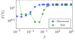
(a) Decomposition using $\eta_{1}$.

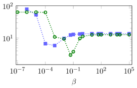
(b) Decomposition using $\eta_{3}$.

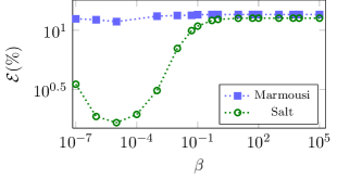
(c) Decomposition using $\eta_{5}$.

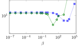
(d) Decomposition using $\eta_{6}$.

Figure 4: Decomposition of the Marmousi and salt velocity models of Figures 3(a) and 3(b) using $N=50$ eigenvectors and following Algorithm 1. The relative error is computed from (20) for four selected formulation of $\eta$ (see Table 1) and different scaling parameter $\beta$.

We then picture the resulting images obtained after the decomposition of both models, see Figures 5 and 6. The pictures illustrate correctly the observations of the tables and the differences between the formulation. The salt model is usually well recovered with all formulations, while the Marmousi model is more hardly discovered, except with $\eta_{1}$, $\eta_{3}$ and $\eta_{6}$. Those three formulations are the only ones able to capture the structures.

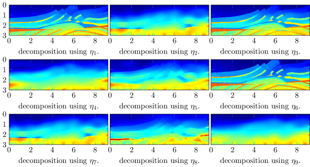
Figure 5: Decomposition of the noise-free Marmousi velocity model of Figure 3(a) using $N=50$, the formulation for $\eta$ are from Table 1 and the respective $\mu$ values extracted from Table 2. The color scale varies between 1500 and 5500m s^-1.

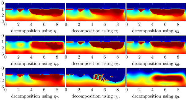
Figure 6: Decomposition of the noise-free salt velocity model of Figure 3(b) using $N=20$, the formulation for $\eta$ are from Table 1 and the respective $\mu$ values extracted from Table 3. The color scale varies between 1500 and 4500m s^-1.

4.2 Decomposition of noisy models (denoising)

We incorporate noise in the representation for getting closer to the reality of applications where few information on the model is available. Hence, we reproduce the model decomposition, this time working with noisy pictures. For every nodal velocity (of Figure 3), we recast the values using an uniform distribution that covers $\pm 20\%$ of the noiseless value. The resulting media are illustrated in Figure 7.

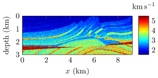
(a) Marmousi velocity model with noise.

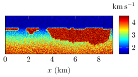
(b) Salt velocity model with noise.

Figure 7: Seismic velocity models of Figure 3 with added noise. For every coefficient, the noisy one is obtained by randomly taking a value between $\pm 20\%$ of the noiseless coefficient.

We apply the model decomposition using the different formulations of $\eta$ and choice of scaling coefficient $\beta$, following the procedure employed for the noiseless model. In Tables 4 and 5, we show the evolution of best relative error with $N$, for the noisy Marmousi and salt models respectively. Here, the relative error is computed from the difference between the noiseless model and the decomposition of the noisy one. The objective of the regularization is to preserve the structures while smoothing out the noise effect.

Table 4: Minimal relative error obtained and associated scaling coefficient: $\mathcal{E}$ ($\beta$). The error is computed with respect to the noiseless model Figure 3(a) but the decomposition uses the noisy model of Figure 7(a). The definition of $\eta$ is given Table 1.

Coeff.	$N=10$	$N=20$	$N=50$	$N=100$	$N=250$
$\eta_{1}$	16% ($10^{-4}$)	15% ($10^{-4}$)	14% ($10^{-7}$)	13% ($10^{-7}$)	11% ($10^{-7}$)
$\eta_{2}$	16% (5.$10^{-2}$)	16% (5.$10^{-2}$)	15% (5.$10^{-2}$)	14% (5.$10^{-2}$)	13% (5.$10^{-2}$)
$\eta_{3}$	16% ($10^{-2}$)	14% ($10^{-3}$)	13% ($10^{-4}$)	12% ($10^{-4}$)	10% ($10^{-4}$)
$\eta_{4}$	16% ($10^{1}$)	16% ($10^{1}$)	16% (5.$10^{1}$)	15% (5.$10^{1}$)	14% ($10^{2}$)
$\eta_{5}$	16% ($10^{-6}$)	16% ($10^{-7}$)	15% ($10^{-7}$)	15% ($10^{-7}$)	14% ($10^{-6}$)
$\eta_{6}$	16% ($10^{2}$)	14% ($10^{3}$)	13% ($10^{4}$)	12% ($10^{4}$)	10% ($10^{4}$)
$\eta_{7}$	16% (5.$10^{-2}$)	16% (5.$10^{-2}$)	15% (5.$10^{-2}$)	14% (5.$10^{-2}$)	13% (5.$10^{-2}$)
$\eta_{8}$	17% (n/a)	16% (n/a)	16% (n/a)	15% (n/a)	14% (n/a)
$\eta_{9}$	17% (n/a)	17% (n/a)	16% (n/a)	16% (n/a)	14% (n/a)

Table 5: Minimal relative error obtained and associated scaling coefficient: $\mathcal{E}$ ($\beta$). The error is computed with respect to the noiseless model Figure 3(b) but the decomposition uses the noisy model of Figure 7(b). The definition of $\eta$ is given Table 1.

Coeff.	$N=10$	$N=20$	$N=50$	$N=100$	$N=250$
$\eta_{1}$	14% ($10^{-6}$)	14% ($10^{-6}$)	11% ($10^{-5}$)	9% ($10^{-5}$)	5% ($10^{-3}$)
$\eta_{2}$	17% (5.$10^{-2}$)	15% (5.$10^{3}$)	11% (5.$10^{-2}$)	8% (5.$10^{-2}$)	6% (5.$10^{-2}$)
$\eta_{3}$	10% ($10^{-4}$)	10% ($10^{-4}$)	8% ($10^{-4}$)	6% ($10^{-4}$)	5% ($10^{-2}$)
$\eta_{4}$	18% ($10^{-3}$)	15% ($10^{0}$)	12% ($10^{-1}$)	10% ($10^{-3}$)	6% ($10^{-3}$)
$\eta_{5}$	17% ($10^{-7}$)	15% (5.$10^{3}$)	12% ($10^{-4}$)	9% ($10^{-7}$)	6% ($10^{-5}$)
$\eta_{6}$	10% ($10^{4}$)	9% ($10^{4}$)	8% ($10^{4}$)	6% (5.$10^{3}$)	5% ($10^{2}$)
$\eta_{7}$	17% (5.$10^{-2}$)	15% ($10^{5}$)	11% ($10^{-2}$)	8% (5.$10^{-2}$)	6% (5.$10^{-2}$)
$\eta_{8}$	18% (n/a)	16% (n/a)	12% (n/a)	9% (n/a)	6% (n/a)
$\eta_{9}$	21% (n/a)	15% (n/a)	13% (n/a)	11% (n/a)	8% (n/a)

The decomposition of noisy pictures requires more eignevectors for an accurate representation. Then, the salt model, with high contrast objects, still behaves better than the many structures of the Marmousi model. For the decomposition of the noisy Marmousi model, none of the formulations really stands out and the error never reaches below 10% using at most $N=250$.

In Figures 8 and 9, we picture the resulting decomposition for the two media. For the decomposition of the Marmousi model, we use $N=200$; and $N=50$ for the salt model. It corresponds to higher values compared to the pictures shown for the noiseless models (Figures 5 and 6).

The decomposition of the salt model remains acceptable, and we easily distinguish the main contrasting object. The smaller objects also appear, in a smooth representation. The formulations using $\eta_{1}$, $\eta_{3}$ and $\eta_{6}$ provide sharper boundary for the contrasting objects, in particular for the upper interface. Regarding the decomposition of the noisy Marmousi model, it illustrates the limitation of the method, where none of the formulations is really able to reproduce the structures, and most edges are lost. In particular, the central part of the model is mostly missing and the amplitude of the values has been reduced. It seems that $\eta_{1}$, $\eta_{3}$ and $\eta_{6}$ are slightly more robust and gives (relatively speaking) the best results. To conclude, these three formulations appear less sensitive (for both media) to noise than the other ones.

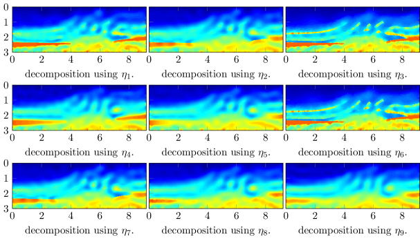
Figure 8: Decomposition of the Marmousi velocity model of Figure 7(a) using $N=200$ and the formulations of $\eta$ from Table 1. The selected value of $\beta$ for every method corresponds to the value given in Table 4. The color scale follows the one of Figure 7(a) with values between 1500 and 5500m s^-1.

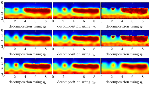
Figure 9: Decomposition of the salt velocity model of Figure 7(b) using $N=50$ and the formulations of $\eta$ from Table 1. The selected value of $\beta$ for every method corresponds to the value given in Table 5. The color scale follows the one of Figure 7(b) with values between 1500 and 4500m s^-1.

In the context of image decomposition, we have can draw the following conclusions for the the decomposition using the basis of eigenvectors.

• The method is efficient to represent media with contrasting shapes (e.g., salt domes), even when noise is contained in the images. In this case, the choice of $\eta$ does not really affect the representation of the objects, and all methods behave quite well, see Figure 9.

• The performance of the decomposition strongly depends on the media, and diminishes with thin structures as in the Marmousi model. In this case, an appropriate choice of formulation ($\eta_{1}$, $\eta_{3}$, $\eta_{6}$ from Table 2) can provide the accurate representation for noise-free picture but when incorporating noise, the performance deteriorates and the edge contrasts are lost.

4.3 Sub-surface salt with layers: SEAM Phase I model

We have seen that the decomposition behaves well when a contrasting object with sharp contrast belongs to the medium, while structures/layers are hardly represented. We pursue our investigation with a common geophysical configuration where both salt-domes and layers exist in the subsurface. We use a velocity model extracted from the SEAM (SEG Advanced Modeling Program ) Phase I benchmark a consider a medium of size $17.5\times 3.75$ km. Per consistency with the previous experiment, it is represented using a grid of $921\times 301$ points, see Figure 10.

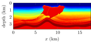
(a) Noise-free velocity model.

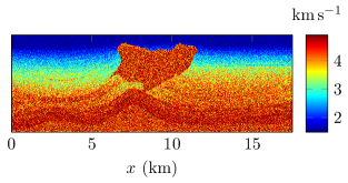
(b) Velocity model with noise.

Figure 10: SEAM velocity model of size $17.5\times 3.75$ km, represented on a Cartesian grid of size $921\times 301$.

Similarly to our previous experiment, we investigate the noiseless model and a noisy one, which incorporates $\pm 20$ % error. The relative error and corresponding scaling coefficients for both models are given in Tables 6 and 7. The relative error is of a few percent for high $N$, and we observe important differences between the formulation. Here, $\eta_{8}$, $\eta_{9}$ and $\eta_{4}$ give the worst results.

We further illustrate the decomposition in Figure 11, using $\eta_{1}$ only for the sake of clarity.

Table 6: Minimal relative error obtained and associated scaling coefficient: $\mathcal{E}$ ($\beta$), for the decomposition of the SEAM model Figure 10(a). The definition of $\eta$ is given Table 1.

Coeff.	$N=10$	$N=20$	$N=50$	$N=100$	$N=200$
$\eta_{1}$	4% ($10^{-6}$)	3% ($10^{-6}$)	3% ($10^{-6}$)	2% ($10^{-6}$)	2% ($10^{-7}$)
$\eta_{2}$	8% (5.$10^{-2}$)	6% (5.$10^{-2}$)	5% ( $10^{-1}$)	3% ( $10^{-2}$)	3% ( $10^{-2}$)
$\eta_{3}$	6% ($10^{-3}$)	5% ($10^{-2}$)	4% ($10^{-3}$)	3% ($10^{-2}$)	2% ($10^{-3}$)
$\eta_{4}$	10% ( 5)	9% ( 10)	7% ($10^{2}$)	6% ($10^{2}$)	5% ( 5)
$\eta_{5}$	7% ($10^{-7}$)	6% ($10^{-6}$)	4% ($10^{-6}$)	3% ($10^{-5}$)	3% ($10^{-5}$)
$\eta_{6}$	6% ($10^{3}$)	5% ($10^{2}$)	4% ($10^{3}$)	3% ($10^{2}$)	2% ($10^{3}$)
$\eta_{7}$	8% ($5.10^{-2}$)	6% ($5.10^{-2}$)	5% ($10^{-1}$)	4% ($5.10^{-2}$)	3% ($5.10^{-2}$)
$\eta_{8}$	18% (n/a)	17% (n/a)	14% (n/a)	12% (n/a)	9% (n/a)
$\eta_{9}$	12% (n/a)	10% (n/a)	7% (n/a)	7% (n/a)	6% (n/a)

Table 7: Minimal relative error obtained and associated scaling coefficient: $\mathcal{E}$ ($\beta$), for the decomposition of the SEAM model Figure 10(b). The definition of $\eta$ is given Table 1.

[ht!] Coeff. $N=10$ $N=20$ $N=50$ $N=100$ $N=200$ $\eta_{1}$ 11% ($10^{-3}$) 8% ($10^{-3}$) 6% ($10^{-6}$) 5% ($10^{-7}$) 4% ($10^{-5}$) $\eta_{2}$ 8% ($5.10^{-2}$) 6% ($5.10^{-2}$) 6% ($5.10^{-2}$) 4% ($5.10^{-2}$) 3% ($5.10^{-2}$) $\eta_{3}$ 6% ($10^{-2}$) 5% ($10^{-2}$) 4% ($10^{-3}$) 4% ($10^{-3}$) 4% ($10^{-2}$) $\eta_{4}$ 11% ($10^{-2}$) 10% ($0.5$) 7% ($10^{-4}$) 6% ($10^{-3}$) 5% ($10^{-3}$) $\eta_{5}$ 11% ($10^{-4}$) 10% ($1$) 7% ($10^{-2}$) 6% ($10^{-4}$) 5% ($10^{-5}$) $\eta_{6}$ 8% ($10^{2}$) 6% ($10^{2}$) 5% ($10^{2}$) 4% ($10^{2}$) 3% ($10^{2}$) $\eta_{7}$ 8% ($5.10^{-2}$) 6% ($5.10^{-2}$) 6% ($5.10^{-2}$) 4% ($5.10^{-2}$) 3% ($5.10^{-2}$) $\eta_{8}$ 11% (n/a) 11% (n/a) 7% (n/a) 6% (n/a) 5% (n/a) $\eta_{9}$ 12% (n/a) 10% (n/a) 7% (n/a) 7% (n/a) 6% (n/a)

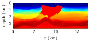
(a) Decomposition of noiseless model using $N=20$.

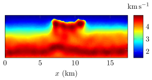
(b) Decomposition of noisy model using $N=100$.

Figure 11: Decomposition of the SEAM Phase I velocity model of Figure 10 using $\eta_{1}$. The relative errors for all formulations can be found in Tables 6 and 7.

This model, which encompasses salt and layers, is well recovered with a decomposition using $N=20$ when there is no noise. In case of noise, it needs higher $N$ and the contrasting shapes are smoothed out. Nonetheless, compared to the Marmousi model, the decomposition is able to capture the main features.

5 Experiments of reconstruction with FWI

In this section, we perform seismic imaging following the FWI Algorithm 2 for the identification of the subsurface physical parameters. We focus on media encompassing salt domes, as we have shown that the decomposition is more appropriate, and it also gives a more challenging configuration in seismic applications. We follow a seismic context, where the forward problem is given by (2) and the data are restricted to be acquired near the surface (see Figure 1). The challenges of our experiments is threefold:

1. the recovery of salt domes is recognized to be difficult (Barucq et al., 2019a);

2. we consider an initial guess that has no information on the subsurface structures and where the background velocity amplitude is incorrect.

3. we avoid the use of the (unrealistically) low frequencies (below $2$ Hz in exploration seismic).

5.1 Reconstruction of two-dimensional salt model

We first consider a two-dimensional salt model of size $9.2\times 3$ km, which consists in three domes, see Figure 13(a). We generate the data using $91$ sources and $183$ receivers (i.e. data points) per source. Both devices are located near the surface: the sources are positioned on a line at $20$ m depth and the receivers at $80$ m depth. In order to establish a realistic situation despite having a synthetic experiment, the data are generated in the time-domain and we incorporate white noise in the measurements. The level of the signal to noise ratio in the seismic trace is of $10$ dB, the noise is generated independently for all receivers record associated with every source. Then we proceed to the discrete Fourier transform to obtain the signals to be used in the reconstruction algorithm. In Figure 12, we show the time-domain data with noise and the corresponding frequency data for one source, located at $20$ m depth, in the middle of the $x$-axis.

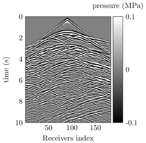
(a) Time-domain trace with included noise.

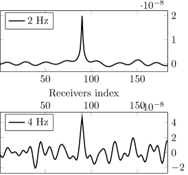
(b) Real parts of the discrete Fourier transform.

Figure 12: Data associated with a single centered source. The data are first generated in the time-domain, then we incorporate white noise and proceed to the Fourier transform. In this experiment, the complete seismic acquisition is composed of $91$ independent sources and $183$ receivers for each source.

For the reconstruction of the salt dome model, the starting and true model are given in Figure 13. We do not assume any a priori knowledge of the contrasting object in the subsurface, and start with a one-dimensional variation, which has a drastically lower amplitude (i.e., the background velocity is unknown).

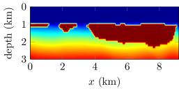
(a) Target model.

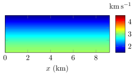
(b) Initial guess for inversion.

Figure 13: Target model and starting model for FWI. The models are of size $9.2\text{\text{km}}\times 3\text{\text{km}}$. The initial model corresponds to a one-dimensional variation of low velocity.

5.1.1 Fixed decomposition, single frequency reconstruction

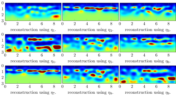
Figure B1: Reconstruction of the salt velocity model from starting medium Figure 13(b) (with the same color scale) using $2$ Hz frequency data. The eigenvector decomposition employs $N=100$ and the formulations of $\eta$ from Table 1.

We first only use $2$ Hz frequency data, and perform $180$ iterations for the minimization. In Figure 14, we show the reconstruction where the decomposition has not been employed, i.e. the model representation follows the original piecewise constant decomposition of the model (one value per node). In Figure 15, we compare the reconstruction using Algorithm 2 for the different formulations of $\eta$ given in Table 1, using a fixed $N=50$. We use $N=100$ for Figure 16. For the sake of clarity, we focus on $\eta_{3}$ (the most effective formulation), and $\eta_{8}$ (which relates to the Total Variation regularization) and move the complete pictures with comparison of all formulations in Appendix B, Figure B1 for $N=100$.

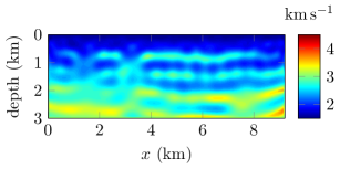
Figure 14: Reconstruction of the salt velocity model from the starting medium Figure 13(b) using $2$ Hz frequency data. The reconstruction does not apply eigenvector decomposition. The model is parametrized following the domain discretization, using piecewise constant representation with one value per node on a $\text{921}\times\text{301}$ grid.

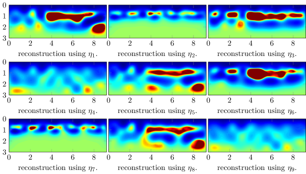
Figure 15: Reconstruction of the salt velocity model from the starting medium Figure 13(b) using $2$ Hz frequency data. The eigenvector decomposition employs $N=50$ and the formulations of $\eta$ from Table 1. It uses the same color scale as Figure 13.

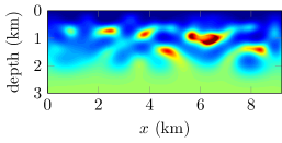
(a) Reconstruction using $\eta_{3}$.

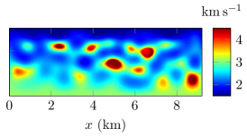
(b) Reconstruction using $\eta_{8}$ (Total Variation).

Figure 16: Reconstruction of the salt velocity model from the starting medium Figure 13(b) using $2$ Hz frequency data. The eigenvector decomposition employs $N=100$. The comparison of all formulations of $\eta$ (Table 1) is pictured in Appendix B, Figure B1.

We observe that

• the traditional FWI algorithm (without decomposition), see Figure 14, fails to recover any dome. It only shows some thin layers of increasing velocity, with amplitudes much lower than the original ones.

• The decomposition using $N=50$ is able to discover the largest object with formulation $\eta_{1}$, $\eta_{3}$, $\eta_{5}$, $\eta_{6}$ and $\eta_{8}$, see Figure 15. The best result is given by $\eta_{3}$ which recovers the three domes; while $\eta_{1}$, $\eta_{5}$ and $\eta_{8}$ show artifacts in the lower right corner. The other decompositions fail. We note that, due to the lack of velocity background information, the positions of the domes are slightly above the correct ones to compensate for the low travel times.

• In this experiment, the method behaves much better with a restrictive number of eigenvectors. With $N=100$ (Figures 16 and B1), the iterative reconstruction only results in artifacts. The restrictive number of eigenvectors provides a regularization of the problem by reducing the number of parameters, which is crucial. For instance, the stability is known to deteriorate exponentially with the number of parameters in the piecewise constant case (Beretta et al., 2016).

Opposite to the decomposition of images (Section 4), the quantitative reconstruction using a model represented with a basis of eigenvectors from a diffusion PDE shows drastic differences between the formulations, where the procedure can fail depending on the choice of $\eta$. In addition, the number of eigenvectors for the representation has to be carefully selected, see Subsection 5.3.

5.1.2 Experiments with increasing $N$ and multiple frequencies

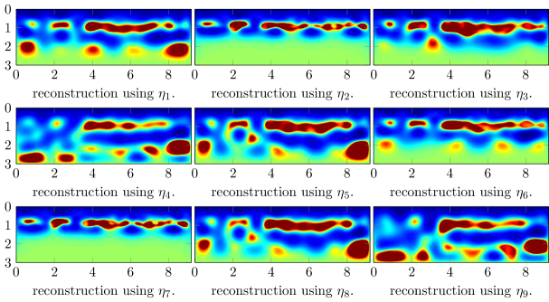
Figure B2: Experiment 2 of Table 8 (multiple $N$, single frequency data) for the reconstruction of the salt velocity model from starting medium Figure 13(b) (with the same color scale), the formulations of $\eta$ follow Table 1.

We investigate the performance of the eigenvector decomposition for multiple frequency data, and with progressive evolution of the number of eigenvectors in the representation $N$. We have a total of four different experiments, which are summarized in Table 8. The reconstructions, for $\eta_{3}$ and $\eta_{8}$, are shown Figure 17. The results for all $\eta$ of Table 1 are pictured in Appendix B, Figures B2, B3 and B4.

Table 8: List of experiments for the reconstruction of the two-dimensional salt dome model (Figure 13(b)). For each combination of frequency and associated number of eigenvectors $N$ in the decomposition, $30$ iterations are performed ($n_{\text{iter}}$ in Algorithm 2).

	frequency list	list of $N$	total iterations	Reference
Experiment 1	$2$ Hz	50	180	Figures 15, B1
Experiment 2	$2$ Hz	$\{50,60,70,80,90,100\}$	180	Figures 17, B2
Experiment 3	$\{2,3,4,5\}$Hz	50	120	Figures 17, B3
Experiment 4	$\{2,3,4,5\}$Hz	$\{50,60,70,80\}$	120	Figures 17, B4

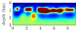
(a) Reconstruction Experiment 1 using $\eta_{3}$ and 180 iterations.

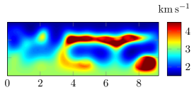
(b) Reconstruction Experiment 1 using $\eta_{8}$ (Total Variation) and 180 iterations.

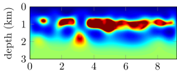
(c) Reconstruction Experiment 2 using $\eta_{3}$.

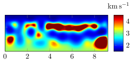
(d) Reconstruction Experiment 2 using $\eta_{8}$ (Total Variation).

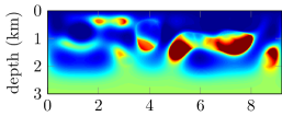
(e) Reconstruction Experiment 3 using $\eta_{3}$.

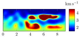
(f) Reconstruction Experiment 3 using $\eta_{8}$ (Total Variation).

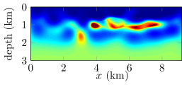
(g) Reconstruction Experiment 4 using $\eta_{3}$.

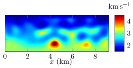
(h) Reconstruction Experiment 4 using $\eta_{8}$ (Total Variation).

Figure 17: Results of Experiments 2, 3 and 4 of Table 8 for the reconstruction of the salt velocity model Figure 13. The comparison of all formulations of $\eta$ (Table 1) is pictured in Appendix B, Figures B2, B3 and B4.

From these experiments using multiple $N$ and/or frequency contents, we observe the performance of the method. The best results are obtained using a single $2$ Hz frequency with either progression of increasing $N$ or constant $N$: Experiments 2 and 1. The progression of $N$, Experiment 2, appears the most robust.

In this experiment, using multiple frequencies does not improve the results. It is probably due to the lack of knowledge of the velocity background which prevents us from recovering finer scale (i.e., kinematic error, Bunks et al. (1995)). In particular, local minima in the misfit functional become more and more prominent in the high-frequency regime (Bunks et al., 1995; Barucq et al., 2019b). We illustrate the performance of the reconstruction with the results in the data-space: in Figure 18, we show the time-domain seismograms for the true, starting and reconstructed velocity models. We observe that when we filter out frequencies above 2 Hz (first line of Figure 18), the trace from the reconstructed model is indeed very similar to the measured one. However, when encompassing all frequency contents (bottom line of Figure 18), important differences arise, in particular, one can see the travel time of the first reflection which is earlier with the recovered model. This indicates that the location of the salt in the reconstructed velocity is above its ‘true’ position.

Then, while we incorporate the higher frequency in the minimization procedure, the FWI is not amenable to improve the results (see Figure 17) and it is most likely due to the missing velocity background which is not improved during the first iterations, and still missing. In Figure 19, we show the frequency-domain data at $2$ and $4$ Hz: the observed data at $2$ Hz are accurately obtained with the model reconstructed with the decomposition in eigenvectors, which confirms the pertinence of the method. Interestingly, at $4$ Hz, while the frequency is not even used in the inversion scheme (we only use $2$ Hz for Figure 17(a)), we already have a good correspondence near the source and only the parts further away show a shift. In order to overcome the issue of recovering the background velocity, one would need lower frequency content, or one could employ alternative strategies, such as the MBTT method, based upon the decomposition of the background velocity model and the reflectivity (Clément et al., 2001). Here, the decomposition in eigenvectors appropriately recover the reflectivity part (better than traditional FWI), but the background model remains missing.

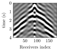
(a) Measured seismic trace, from the model of Figure 13(a), filtering out the frequency content above $2$ Hz.

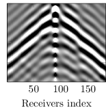
(b) Seismic trace from the reconstructed velocity model of Figure 17(a), filtering out the frequency content above $2$ Hz.

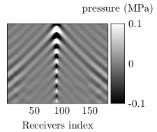
(c) Seismic trace from the starting velocity model, Figure 13(b), filtering out the frequency content above $2$ Hz.

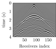
(d) Measured seismic trace, from the model of Figure 13(a).

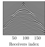
(e) Seismic trace from the reconstructed velocity model of Figure 17(a).

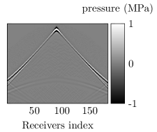
(f) Seismic trace from the starting velocity model, Figure 13(b).

Figure 18: Comparison of the time-domain seismic traces for a central shot using different velocity models of the salt medium reconstruction experiment.

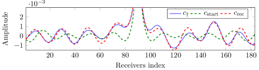
(a) Comparison of the real parts of the pressure fields at $2$ Hz.

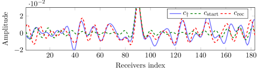
(b) Comparison of the real parts of the pressure fields at $4$ Hz.

Figure 19: Comparisons of the frequency-domain data (pressure field) at the receivers location for a central source. We compare the data obtained from the target wave speed with salt of Figure 13(a), the starting wave speed of Figure 13(b) and the reconstruction of Figure 17(a). Those three models are respectively denoted $c_{\dagger}$, $c_{\text{start}}$ and $c_{\text{rec}}$.

5.1.3 On the choice of the number of eigenvectors

We have shown in Figures 15 and 16 that one should take an initial $N$ relatively low for the reconstruction algorithm to succeed. It remains to verify if the appropriate $N$ can be selected ‘a priori’, or based upon minimal experiments. In Figure 20(a), we show the evolution of the misfit functional with thirty iterations, for different values of $N$, from $10$ to $250$. We compare, in Figure 20(b), with the progression of $N$, which follows Experiment 2 of Table 8.

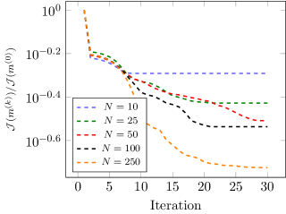
(a) Using fixed $N$.

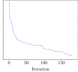
(b) Using progression of $N$ (from $50$ to $100$), every $30$ iterations, following Experiment 2 of Table 8.

Figure 20: Evolution of the misfit functional (scaled with the first iteration value) with iterations depending on the choice of $N$, using $2$ Hz frequency.

From Figure 20(a), we see that all of the choices of $N$ have the same pattern: first the decrease of the functional and then its stagnation. We notice that the good choice for $N$ is not reflected by the misfit functional. Indeed, it shows lower error for larger $N$, while they are shown to result in erroneous reconstructions (Figure 16 compared to Figure 15). It is most likely that using larger $N$ leads to local minima and/or deteriorates the stability (see, for the piecewise constant case, Beretta et al. (2016)). It results in the false impression (from the misfit functional point of view) that it would improve the efficiency of the method. Using a progression of $N$, Figure 20(b), eventually gives the same misfit functional value than the large $N$, but it needs more iterations. This increase of iterations and ‘slow’ convergence is actually required, because it leads to an appropriate reconstruction, see Figure 17.

Therefore, we cannot anticipate a good choice for $N$ a priori (with a few evaluation of the misfit functional). the guideline we propose, as a safe and robust approach, is the progression of increasing $N$, from low to high: it costs more in terms of iterations, but it converges properly.

5.2 Reconstruction of the SEAM Phase I model

We now consider the recovery of the SEAM Phase I model, which is expected to be more challenging as it contains both a salt-dome and sub-salt layers. The starting model for the reconstruction is shown in Figure 21, where, for the sake of clarity, we also picture the reference model which was previously used for the decomposition. This medium is of size $17.5\times 3.75$ km and the starting model we use is a smooth version of the reference one, where the contrasting objects and layers are missing.

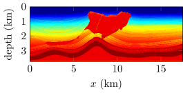
(a) Target model.

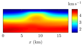
(b) Initial guess for inversion.

Figure 21: Target model and starting model for FWI, of size $17.5\times 3.75$ km.

We follow the same configuration as in the previous experiment: the data are generated in the time-domain, and noise is incorporated to the seismograms using a signal-to-noise ratio of 10 dB. Next, we proceed with the discrete Fourier-transform to employ the iterative procedure with time-harmonic waves. In this experiment, the smallest available frequency is $2$ Hz.

For the sake of conciseness, we only present the reconstruction results with the the representation using $\eta_{3}$ (which was the most efficient). We follow a slow increase of $N$ in a fixed basis (analogous to Experiment 2 of Table 8) which was the more stable approach. The reconstruction using $2$ Hz is shown in Figure 22.

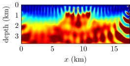
(a) Reconstruction after $180$ iterations without using the eigenvector decomposition.

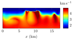
(b) Reconstruction using eigenvector decomposition with $\eta_{3}$ and a sequence $N=\{25,35,50,60,70,80\}$ with $30$ iterations for each, i.e. a total of 180 iterations.

Figure 22: Reconstruction of the SEAM phase I model from an initially smooth model, see Figure 21, using $2$ Hz frequency data.

We observe that the standard FWI algorithm gives artifacts over the medium, with oscillatory patterns, in particular on the sides. On the other hand, the reconstruction using the representation based upon the eigenvector decomposition is stable, and is able to capture accurately the upper boundary of the salt dome. Because of the frequency employed, only the long wavelengths are recovered at this stage. In Figure 23, we further illustrate the recovery by showing the frequency-domain data at $2$ Hz frequency using the different wave speed models. We can see that the data from the starting model are out of phase as soon as we move away from the source, with cycle-skipping effects. However, the reconstruction using the eigenvector decomposition is able to retrieve this information and accurately capture the oscillations of the signal, and only the amplitude is inaccurate.

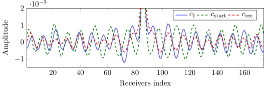
(a) Comparison of the real parts of the pressure fields.

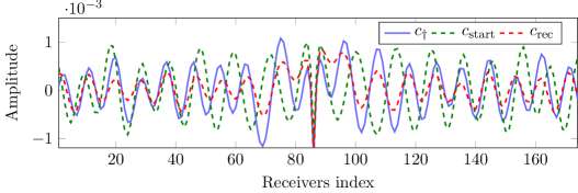
(b) Comparison of the imaginary parts of the pressure fields.

Figure 23: Comparisons of the frequency-domain data (pressure field) at the receivers location for a centrally located source at $2$ Hz frequency for the SEAM Phase I wave speed of Figure 21(a), the starting wave speed of Figure 21(b) and the reconstruction using the eigenvector decomposition, Figure 22(b). Those three models are respectively denoted $c_{\dagger}$, $c_{\text{start}}$ and $c_{\text{rec}}$.

We now continue the procedure using increasing frequencies. Because of the smoothing effect of the decomposition, we employ the algorithm without the eigenvector representation (alternatively, one could use the decomposition but with large $N$). Therefore, the velocity model obtained from the FWI with eigenvector decomposition of Figure 22(b) is used as an initial model for restarted FWI with multiple frequencies, from $2$ to $10$ Hz (we use the sequential progression advocated by Barucq et al. (2019a)). Eventually, the reconstruction after $10$ Hz iterations is pictured in Figure 24.

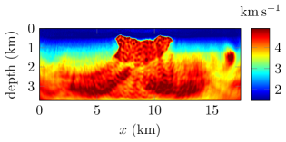
Figure 24: Reconstruction of the SEAM phase I model starting from the reconstruction obtained with eigenvector decomposition of Figure 22(b), using data of frequency from $2$ to $10$ Hz, with 30 iterations per (sequential) frequency.

The reconstruction is able to capture the finer details of the velocity model: the salt dome is clearly defined, and the sub-salt layer starts to appear. Therefore, the eigenvector decomposition method can also serve to build initial models for the FWI algorithm, where it appears as an interesting alternative to overcome the lack of low frequency. To illustrate the different steps of the reconstruction, we show the time-domain seismograms at the different stages of the reconstruction in Figure 25 (while the $2$ Hz frequency-domain data are given in Figure 23). We compare the traces resulting from the initial and true wave speed models, from the partial reconstruction obtained with the eigenvector decomposition (Figure 22(b)), and from the final reconstruction (Figure 24).

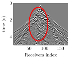
(a) Measured seismic trace corresponding to the SEAM Phase I model of Figure 21(a).

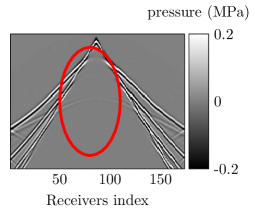
(b) Seismic trace corresponding to the starting model of Figure 21(b).

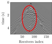
(c) Seismic trace corresponding to the partial reconstruction using the eigenvector decomposition, Figure 22(b).

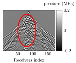
(d) Seismic trace corresponding to the final reconstruction given Figure 24.

Figure 25: Comparison of the time-domain seismic traces for a central shot using different velocity models.

The trace that uses the starting model mainly shows the first arrivals, with some minor reflections coming from the smoothing of the salt dome. The one using the partial reconstruction with eigenvenctor decomposition and only the $2$ Hz data accurately resolves the main multiple reflections between the salt upper boundary and the surface (the thick line in the center of the red ellipses in Figure 25) but it misses the events of smaller importance. Eventually, the final reconstruction, that uses up to $10$ Hz data contents is able to reproduce some of the events of smaller amplitudes. We also note that the amplitude of the trace for the final reconstruction is slightly high, which indicates that the contrasts are even too strong.

5.3 Implementation of the method

The eigenvector decomposition for the model representation depends on different choices of parameters, and it is not trivial to efficiently implement the method in the iterative reconstruction procedure. From the experiments we have carried out, we propose the following strategy.

1. Regarding the choice of weighting coefficient, $\eta_{3}$ from Geman & Reynolds (1992) is the most efficient in these applications, and supersedes the standard Total Variation approach (i.e., $\eta_{8}$).

Secondly, the difficulty resides in the number of eigenvectors to take for the decomposition: $N$. More important, it appears that the misfit functional does not provide us with a good indication (see Figure 20).

1. The number of eigenvector $N$ for the decomposition should initially takes a low value, and progressively evolves to higher values with iterations. It may not be the fastest convergence, but it is the most robust approach.

Finally, the reconstruction can serve as an initial model for multi-frequency data:

1. the (partial) reconstruction with eigenvector decomposition is used as a starting model for multi-frequency algorithm. It allows the recovery of the finer details, which depend on the smaller wavelengths and where the smoothing effect is misleading.

Namely, the decomposition is particularly efficient to overcome the lack of low-frequency in the data.

5.4 Three-dimensional experiment

The method extends readily for three-dimensional model reconstruction, simply incurring a larger computational cost (as larger matrices are involved for the eigenvector decomposition and the forward problem discretization). We proceed with a three-dimensional experiment, where we consider a subsurface medium of size $2.46\times 1.56\times 1.2$ km, encompassing several salt domes, illustrated in Figure 26. The seismic acquisition consists in 96 sources, positioned on a two-dimensional plane at 10 m depth; one thousand receivers are positioned at 100 m depth. Similar to the previous experiments, the data are first generated in the time-domain and we incorporate noise before we proceed to the Fourier transform. Figure 28 shows the time-domain data associated with a centrally located source, and the corresponding Fourier transform at $5$ Hz frequency. For the reconstruction, we start with a one-dimensional variation, in depth only, where none of the objects is intuited, see Figure 27, and the velocity background is incorrect.

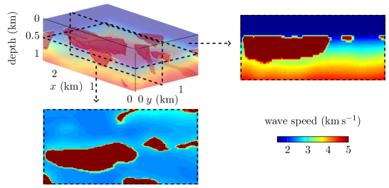
Figure 26: Three-dimensional model incorporating contrasting objects. The domain is of size $2.46\times 1.56\times 1.2$ km. We highlight a horizontal section at $550$ m depth and vertical section at $y=670$ m.

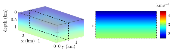
Figure 27: Initial model taken for the reconstruction of the three-dimensional medium with vertical section at $y=670$ m. It consists in a one-dimensional variation in depth.

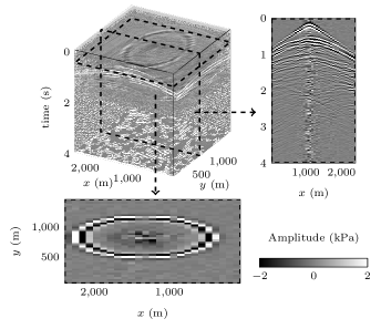
(a) Time-domain measurements with noise.

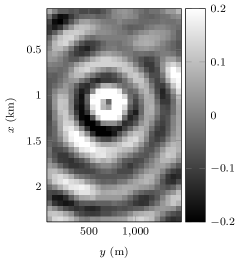
(b) Fourier transform at $5$ Hz.

Figure 28: Time-domain data and corresponding Fourier transform at $5$ Hz frequency. The three-dimensional trace corresponds with the evolution receivers recordings (positioned on a $2$D map in the $x$–$y$ plane) with time. There are $1000$ data points per time step (i.e. 1000 receivers on the domain) and we highlight sections at fixed time ($0.5$ s) and for a line of receivers (positioned at $y=710$ m).

In Figure 29, we show the reconstruction without employing the eigenvector decomposition, where the wave speed has a piecewise constant representation on a $124\times 79\times 61$ nodal grid. We only use $5$ Hz frequency data, and $30$ iterations. Next, we employ the eigenvector model representation with Algorithm 2. Following the discussion in Subsection 5.3, we select $\eta_{3}$, which is the most robust, and try two situations:

• single frequency ($5$ Hz), fixed $N$ reconstruction using $\eta_{3}$, $N=50$ and $30$ iterations, the final reconstruction is Figure 30;

• single frequency ($5$ Hz), multiple $N$ reconstruction using $\eta_{3}$, $N=\{20,30,50,75,100\}$ and $30$ iterations per $N$, i.e. $180$ iterations in total: the final reconstruction is Figure 31.

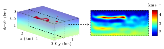
Figure 29: Velocity model reconstruction with vertical section at $y=670$ m, from the starting medium Figure 27 using $5$ Hz frequency data. The reconstruction does not apply the eigenvector decomposition. The model is parametrized following the domain discretization, using piecewise constant representation with one value per node on a $\text{124}\times\text{79}\times\text{61}$ grid.

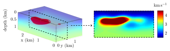
Figure 30: Velocity model reconstruction with vertical section at $y=670$ m, from the starting medium Figure 27 using $5$ Hz frequency data. The reconstruction applies the eigenvector decomposition with $\eta_{3}$ and $N=50$ with $30$ iterations, see Algorithm 2.

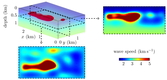
Figure 31: Velocity model reconstruction with vertical section at $y=670$ m and horizontal section at $550$ m depth, from the starting medium Figure 27 and using $5$ Hz frequency data. The reconstruction applies the eigenvector decomposition with $\eta_{3}$ and progression of $N=\{20,30,50,75,100\}$, with 30 iterations per $N$, see Algorithm 2.

For visualization, we focus on the two-dimensional vertical and horizontal sections which illustrate the positions and shapes of the objects. This experiment is consistent with the two-dimensional results, and we observe the following.

• The classical FWI reconstruction fails to discover the subsurface objects, with only a narrow layer, misplaced, see Figure 29.

• The reconstruction with the representation with eigenvector decomposition is able to accurately capture the largest subsurface salt domes, see Figures 30 and 31.

• The best results are obtained when we use the progression of $N$, with a single frequency, see Figure 31. The main salt dome is captured and smaller ones start to appear, including near the boundary. Using a single $N$ is also a good candidate, Figure 30, as it necessitates much less iterations ($30$ instead of $180$) hence less computational time.

6 Conclusion

In this paper, we have investigated the use of a representation based upon a basis of eigenvectors for image decomposition and quantitative reconstruction in the seismic inverse problem, using two and three-dimensional experiments. We have implemented several diffusion coefficients, and compared their performance, depending on the target medium.

1. In the context of image decomposition, the case of contrasting objects (salt domes) is clearly more appropriate than the layered media (such as Marmousi). All of the diffusion coefficients behave well and provide satisfactory results for salt domes image decomposition, even in the presence of noise.

2. For the decomposition of images with layered patterns, only a few formulations perform well ($\eta_{1}$, $\eta_{3}$, $\eta_{6}$). It would be interesting to investigate further the performance of anisotropic or directional diffusion coefficients, mentioned by Weickert (1998); Grote & Nahum (2019).

Next, we have considered the quantitative reconstruction procedure in seismic, where only partial, backscattered (i.e. reflection) data are available, from one side illumination. We have probed the performance of the method by considering initial guesses with minimal a priori information, and by avoiding the low frequency data, which are not accessible in seismic applications. In this context, the FWI algorithm based upon the eigenvector model representation has shown promising results of subsurface $3$D salt dome media. The method only requires the preliminary computation of the basis of eigenvectors associated with the diffusion operator, and a trivial modification of the gradient computation. Namely, the overall additional cost of the method remains marginal compared to the cost of FWI. Our findings are the following.

1. For reconstruction, the result depends on the choice of diffusion coefficient. We recommend $\eta_{3}$, from Geman & Reynolds (1992), which was the most robust in our applications, even with a fixed $N$ and a few iterations.

2. We have shown that the choice of $N$ is not trivial, and one cannot rely on the misfit functional evaluation. Therefore, we have proposed a progression of increasing $N$, which appears to stabilize the reconstruction.

3. Because the method has a smoothing effect, it focuses on the long wavelength structures. Thus, the reconstruction using the decomposition can serve as an initial model to iterate with higher frequency contents, in order to improve the resolution.

Following these analyses, some difficulties remain regarding the optimal choice of parameters. For instance, it is possible that $\eta$ has to be selected differently depending on the model (as illustrated with the Marmousi decomposition). Similarly, the scaling coefficient $\beta$ would affect the performance but the acceptable range appears, hopefully, quite large.

For future work, it seems that the lack of background velocity information would not be overcome by the decomposition, possibly resulting in artifacts. Therefore, we envision the use of multiple basis to parametrize the velocity (e.g., using the background/reflectivity decomposition idea of Clément et al. (2001); Barucq et al. (2019b), with a dedicated smooth eigenvector basis to represent the background, and another to represent the reflectors).

Eventually, the method can readily extend to multi-parameter inversion (e.g. for elastic medium), upon taking a separate basis per parameter (e.g. one for each of the Lamé parameters in linear elasticity). However, a more appropriate approach would be the use of joint-basis by, e.g., considering a system of PDE instead of the scalar diffusion operator. We have in mind strategies such that joint-sparsity and tensor decomposition.

Appendix A Two-dimensional reconstruction with evolution of basis

In this appendix, we experiment the re-computation of the eigenvectors basis along with the iterations. We consider two additional experiments, which are derived from Experiments 1 and 2 of Table 8, with one major difference: the set of eigenvectors is recomputed from the current iteration model every $30$ iterations. This is advocated in De Buhan & Kray (2013); Grote & Nahum (2019) where, contrary to our experiments, the background velocity is mostly known.

Therefore, for the $180$ total iterations, the basis are

• computed from the initial model when starting the very first iteration,

• re-computed from the current reconstruction at the beginning of iterations $31$, $61$, $91$, $121$, $151$.

Compared to Algorithm 2, instead of using a fixed ${\boldsymbol{\psi}}_{\text{loc}}$ from the initial model, it is recomputed from the current ${\mathfrak{m}}^{(k)}$. The reconstructions using the update of basis are shown Figures A1 and A2, for $N=50$ and $N=\{50,60,70,80,90,100\}$ respectively.

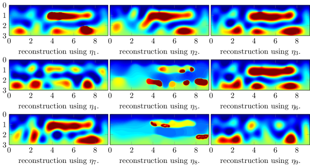
Figure A1: Reconstruction after $180$ iterations from starting medium Figure 13(b) (same color scale) using $2$ Hz data. The decomposition uses $N=50$ and the set of eigenvectors is re-computed every $30$ iterations, from the current iteration model. The formulations of $\eta$ are Table 1.

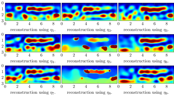
Figure A2: Reconstruction from starting medium Figure 13(b) (same color scale) using $2$ Hz data. The decomposition employs the sequence $N=\{50,60,70,80,90,100\}$ with $30$ iterations per $N$. The set of eigenvectors is re-computed every $30$ iterations, from the current iteration model (i.e. every time we update $N$). The formulations of $\eta$ are from Table 1.

We observe that changing the basis along with the iterations provides similar accuracy of the reconstruction compared to keeping the basis fixed. For some formulations, the salt dome appears slightly larger than with the fixed basis but the artifacts at the bottom are also stronger, with patches of high velocities.

We believe that the difficulty is due to the lack of prior information regarding the velocity background. Namely, the starting model has a background profile of low amplitude compared to the target model, see Figure 13(b). While our reconstruction captures the contrasting object, the background remains mostly erroneous (i.e. $\mathfrak{m}_{0}$ in (14)), impacting the decomposition. Then, when we update the decomposition, the new set of eigenvectors will try to encompass the background variation, creating the bottom artifacts.

Appendix B Extended set of figures

We provide here the reconstructions obtained for all $\eta$ for the two-dimensional salt dome FWI test case of Subsection 5.1.

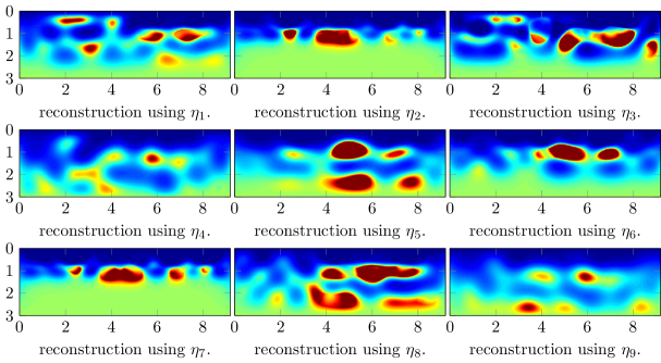
Figure B3: Experiment 3 of Table 8 (single $N$, multiple frequency data) for the reconstruction of the salt velocity model from starting medium Figure 13(b) (with the same color scale), the formulations of $\eta$ follow Table 1.

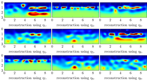
Figure B4: Experiment 4 of Table 8 (multiple $N$, multiple frequency data) for the reconstruction of the salt velocity model from starting medium Figure 13(b) (with the same color scale), the formulations of $\eta$ follow Table 1.

References

- Aghamiry et al. (2019) Aghamiry, H. S., Gholami, A., & Operto, S., 2019. Implementing bound constraints and total-variation regularization in extended full-waveform inversion with the alternating direction method of multiplier: application to large contrast media, Geophysical Journal International, 218(2), 855–872.
- Akcelik et al. (2002) Akcelik, V., Biros, G., & Ghattas, O., 2002. Parallel multiscale gauss-newton-krylov methods for inverse wave propagation, in Supercomputing, ACM/IEEE 2002 Conference, doi: 10.1109/SC.2002.10002.
- Alessandrini & Vessella (2005) Alessandrini, G. & Vessella, S., 2005. Lipschitz stability for the inverse conductivity problem, Adv. in Appl. Math., 35(2), 207–241, doi: 10.1016/j.aam.2004.12.002.
- Alessandrini et al. (2018) Alessandrini, G., de Hoop, M. V., Gaburro, R., & Sincich, E., 2018. Lipschitz stability for a piecewise linear Schrödinger potential from local cauchy data, Asymptotic Analysis, 108(3), 115–149.
- Alessandrini et al. (2019) Alessandrini, G., De Hoop, M. V., Faucher, F., Gaburro, R., & Sincich, E., 2019. Inverse problem for the Helmholtz equation with Cauchy data: reconstruction with conditional well-posedness driven iterative regularization, ESAIM: M2AN, 53(3), 1005–1030, doi: 10.1051/m2an/2019009.
- Alvarez et al. (1992) Alvarez, L., Lions, P.-L., & Morel, J.-M., 1992. Image selective smoothing and edge detection by nonlinear diffusion. ii, SIAM Journal on numerical analysis, 29(3), 845–866.
- Amestoy et al. (2001) Amestoy, P. R., Duff, I. S., L’Excellent, J.-Y., & Koster, J., 2001. A fully asynchronous multifrontal solver using distributed dynamic scheduling, SIAM Journal on Matrix Analysis and Applications, 23(1), 15–41.
- Amestoy et al. (2006) Amestoy, P. R., Guermouche, A., L’Excellent, J.-Y., & Pralet, S., 2006. Hybrid scheduling for the parallel solution of linear systems, Parallel computing, 32(2), 136–156.
- Ammari et al. (2015) Ammari, H., Seo, J. K., & Zhou, L., 2015. Viscoelastic modulus reconstruction using time harmonic vibrations, Mathematical Modelling and Analysis, 20(6), 836–851.
- Anderson et al. (1999) Anderson, E., Bai, Z., Bischof, C., Blackford, S., Demmel, J., Dongarra, J., Du Croz, J., Greenbaum, A., Hammarling, S., McKenney, A., & Sorensen, D., 1999. LAPACK Users’ Guide, Society for Industrial and Applied Mathematics, Philadelphia, PA, 3rd edition.
- Backus & Gilbert (1968) Backus, G. & Gilbert, F., 1968. The resolving power of gross earth data, Geophysical Journal International, 16(2), 169–205.
- Backus & Gilbert (1967) Backus, G. E. & Gilbert, J., 1967. Numerical applications of a formalism for geophysical inverse problems, Geophysical Journal International, 13(1-3), 247–276.
- Bamberger et al. (1979) Bamberger, A., Chavent, G., & Lailly, P., 1979. About the stability of the inverse problem in the 1-D wave equation, Journal of Applied Mathematics and Optimisation, 5, 1–47.
- Barucq et al. (2018) Barucq, H., Faucher, F., & Pham, H., 2018. Localization of small obstacles from back-scattered data at limited incident angles with full-waveform inversion, Journal of Computational Physics, 370, 1–24, doi: 10.1016/j.jcp.2018.05.011.
- Barucq et al. (2019a) Barucq, H., Calandra, H., Chavent, G., & Faucher, F., 2019a. A priori estimates of attraction basins for velocity model reconstruction by time-harmonic Full Waveform Inversion and Data Space Reflectivity formulation, Research Report RR-9253, Magique 3D ; Inria Bordeaux Sud-Ouest ; Université de Pau et des Pays de l’Adour.
- Barucq et al. (2019b) Barucq, H., Chavent, G., & Faucher, F., 2019b. A priori estimates of attraction basins for nonlinear least squares, with application to helmholtz seismic inverse problem, Inverse Problems, 35, 115004 (30pp), doi: https://doi.org/10.1088/1361-6420/ab3507.
- Bednar et al. (2007) Bednar, J. B., Shin, C., & Pyun, S., 2007. Comparison of waveform inversion, part 2: phase approach, Geophysical Prospecting, 55(4), 465–475, doi: 10.1111/j.1365-2478.2007.00618.x.
- Bérenger (1994) Bérenger, J.-P., 1994. A perfectly matched layer for the absorption of electromagnetic waves, Journal of Computational Physics, 114(2), 185 – 200, doi: http://dx.doi.org/10.1006/jcph.1994.1159.
- Beretta et al. (2016) Beretta, E., de Hoop, M. V., Faucher, F., & Scherzer, O., 2016. Inverse boundary value problem for the helmholtz equation: quantitative conditional lipschitz stability estimates, SIAM Journal on Mathematical Analysis, 48(6), 3962–3983.
- Blanc-Féraud et al. (1995) Blanc-Féraud, L., Charbonnier, P., Aubert, G., & Barlaud, M., 1995. Nonlinear image processing: modeling and fast algorithm for regularization with edge detection, in Image Processing, 1995. Proceedings., International Conference on, vol. 1, pp. 474–477, IEEE.
- Bozdağ et al. (2011) Bozdağ, E., Trampert, J., & Tromp, J., 2011. Misfit functions for full waveform inversion based on instantaneous phase and envelope measurements, Geophysical Journal International, 185(2), 845–870, doi: 10.1111/j.1365-246X.2011.04970.x.
- Brandsberg-Dahl et al. (2017) Brandsberg-Dahl, S., Chemingui, N., Valenciano, A., Ramos-Martinez, J., & Qiu, L., 2017. Fwi for model updates in large-contrast media, The Leading Edge, 36(1), 81–87.
- Brossier (2011) Brossier, R., 2011. Two-dimensional frequency-domain visco-elastic full waveform inversion: Parallel algorithms, optimization and performance, Computers & Geosciences, 37(4), 444–455.
- Brossier et al. (2009) Brossier, R., Operto, S., & Virieux, J., 2009. Seismic imaging of complex onshore structures by 2d elastic frequency-domain full-waveform inversion, Geophysics, 74(6), WCC105–WCC118.
- Brossier et al. (2010) Brossier, R., Operto, S., & Virieux, J., 2010. Which data residual norm for robust elastic frequency-domain full waveform inversion?, Geophysics, 75(3), R37–R46, doi: 10.1190/1.3379323.
- Bunks et al. (1995) Bunks, C., Saleck, F. M., Zaleski, S., & Chavent, G., 1995. Multiscale seismic waveform inversion, Geophysics, 60(5), 1457–1473, doi: 10.1190/1.1443880.
- Catté et al. (1992) Catté, F., Lions, P.-L., Morel, J.-M., & Coll, T., 1992. Image selective smoothing and edge detection by nonlinear diffusion, SIAM Journal on Numerical analysis, 29(1), 182–193.
- Charbonnier et al. (1994) Charbonnier, P., Blanc-Féraud, L., Aubert, G., & Barlaud, M., 1994. Two deterministic half-quadratic regularization algorithms for computed imaging, in Image Processing, 1994. Proceedings. ICIP-94., IEEE International Conference, vol. 2, pp. 168–172, IEEE.
- Chavent (1974) Chavent, G., 1974. Identification of functional parameters in partial differential equations, in Identification of Parameters in Distributed Systems, pp. 31–48, eds Goodson, R. E. & Polis, M., ASME, New York.
- Chavent et al. (2015) Chavent, G., Gadylshin, K., & Tcheverda, V., 2015. Reflection fwi in mbtt formulation, in 77th EAGE Conference and Exhibition 2015.
- Chironi et al. (2006) Chironi, C., Morgan, J., & Warner, M., 2006. Imaging of intrabasalt and subbasalt structure with full wavefield seismic tomography, Journal of Geophysical Research: Solid Earth, 111(B5).
- Choi et al. (2008) Choi, Y., Min, D.-J., & Shin, C., 2008. Frequency-domain elastic full waveform inversion using the new pseudo-hessian matrix: Experience of elastic marmousi-2 synthetic data, Bulletin of the Seismological Society of America, 98(5), 2402–2415.
- Clément et al. (2001) Clément, F., Chavent, G., & Gómez, S., 2001. Migration-based traveltime waveform inversion of 2-d simple structures: A synthetic example, Geophysics, 66(3), 845–860.
- De Buhan & Kray (2013) De Buhan, M. & Kray, M., 2013. A new approach to solve the inverse scattering problem for waves: combining the trac and the adaptive inversion methods, Inverse Problems, 29(8), 085009.
- De Buhan & Osses (2010) De Buhan, M. & Osses, A., 2010. Logarithmic stability in determination of a 3d viscoelastic coefficient and a numerical example, Inverse Problems, 26(9), 095006.
- Dubrovin et al. (1992) Dubrovin, B. A., Fomenko, A. T., & Novikov, S. P., 1992. Modern geometry-methods and applications, part i: The geometry of surfaces, transformation groups, and fields.
- Eisenstat & Walker (1994) Eisenstat, S. C. & Walker, H. F., 1994. Globally convergent inexact newton methods, SIAM Journal on Optimization, 4, 393–422.
- Engquist & Majda (1977) Engquist, B. & Majda, A., 1977. Absorbing boundary conditions for numerical simulation of waves, Proceedings of the National Academy of Sciences, 74(5), 1765–1766.
- Esser et al. (2018) Esser, E., Guasch, L., van Leeuwen, T., Aravkin, A. Y., & Herrmann, F. J., 2018. Total variation regularization strategies in full-waveform inversion, SIAM Journal on Imaging Sciences, 11(1), 376–406.
- Evans (2010) Evans, L. C., 2010. Partial differential equations, American Mathematical Society.
- Farmer et al. (1996) Farmer, P., Miller, D., Pieprzak, A., Rutledge, J., & Woods, R., 1996. Exploring the subsalt, Oilfield Review, 8(1), 50–64.
- Faucher (2017) Faucher, F., 2017. Contributions to seismic full waveform inversion for time harmonic wave equations: stability estimates, convergence analysis, numerical experiments involving large scale optimization algorithms, Ph.D. thesis, Université de Pau et Pays de l’Ardour.
- Faucher et al. (2019) Faucher, F., Alessandrini, G., Barucq, H., de Hoop, M. V., Gaburro, R., & Sincich, E., 2019. Full reciprocity-gap waveform inversion in the frequency domain, enabling sparse-source acquisition, arXiv preprint arXiv:1907.09163.
- Fichtner et al. (2008) Fichtner, A., Kennett, B. L., Igel, H., & Bunge, H.-P., 2008. Theoretical background for continental-and global-scale full-waveform inversion in the time–frequency domain, Geophysical Journal International, 175(2), 665–685.
- Gauthier et al. (1986) Gauthier, O., Virieux, J., & Tarantola, A., 1986. Two-dimensional nonlinear inversion of seismic waveforms; numerical results, Geophysics, 51(7), 1387–1403, doi: 10.1190/1.1442188.
- Gee & Jordan (1992) Gee, L. S. & Jordan, T. H., 1992. Generalized seismological data functionals, Geophysical Journal International, 111(2), 363–390.
- Geman & Reynolds (1992) Geman, D. & Reynolds, G., 1992. Constrained restoration and the recovery of discontinuities, IEEE Transactions on Pattern Analysis & Machine Intelligence, (3), 367–383.
- Green (1990) Green, P. J., 1990. Bayesian reconstructions from emission tomography data using a modified em algorithm, IEEE transactions on medical imaging, 9(1), 84–93.
- Grote & Nahum (2019) Grote, M. J. & Nahum, U., 2019. Adaptive eigenspace for multi-parameter inverse scattering problems, Computers & Mathematics with Applications.
- Grote et al. (2017) Grote, M. J., Kray, M., & Nahum, U., 2017. Adaptive eigenspace method for inverse scattering problems in the frequency domain, Inverse Problems, 33(2), 025006.
- Isakov (2006) Isakov, V., 2006. Inverse problems for partial differential equations, vol. 127, Springer.
- Jun et al. (2015) Jun, H., Park, E., & Shin, C., 2015. Weighted pseudo-hessian for frequency-domain elastic full waveform inversion, Journal of Applied Geophysics, 123, 1–17.
- Kalita et al. (2019) Kalita, M., Kazei, V., Choi, Y., & Alkhalifah, T., 2019. Regularized full-waveform inversion with automated salt flooding, Geophysics, 84(4), R569–R582.
- Kaltenbacher (2018) Kaltenbacher, B., 2018. Minimization based formulations of inverse problems and their regularization, SIAM Journal on Optimization, 28(1), 620–645.
- Kern (2016) Kern, M., 2016. Numerical Methods for Inverse Problems, John Wiley & Sons.
- Kirsch (1996) Kirsch, A., 1996. An introduction to the mathematical theory of inverse problems, Applied mathematical sciences, Springer, New York.
- Köhn et al. (2012) Köhn, D., De Nil, D., Kurzmann, A., Przebindowska, A., & Bohlen, T., 2012. On the influence of model parametrization in elastic full waveform tomography, Geophysical Journal International, 191(1), 325–345.
- Lailly (1983) Lailly, P., 1983. The seismic inverse problem as a sequence of before stack migrations, in Conference on Inverse Scattering: Theory and Application, pp. 206–220, ed. Bednar, J. B., Society for Industrial and Applied Mathematics.
- Lehoucq & Sorensen (1996) Lehoucq, R. B. & Sorensen, D. C., 1996. Deflation techniques for an implicitly restarted arnoldi iteration, SIAM Journal on Matrix Analysis and Applications, 17(4), 789–821.
- Lions & Mitter (1971) Lions, J. L. & Mitter, S. K., 1971. Optimal control of systems governed by partial differential equations, vol. 1200, Springer Berlin.
- Lobel et al. (1997) Lobel, P., Blanc-Féraud, L., Pichot, C., & Barlaud, M., 1997. A new regularization scheme for inverse scattering, Inverse Problems, 13(2), 403.
- Loris et al. (2007) Loris, I., Nolet, G., Daubechies, I., & Dahlen, F., 2007. Tomographic inversion using l1-norm regularization of wavelet coefficients, Geophysical Journal International, 170, 359–370.
- Loris et al. (2010) Loris, I., Douma, H., Nolet, G., Daubechies, I., & Regone, C., 2010. Nonlinear regularization techniques for seismic tomography, Journal of Computational Physics, 229, 890–905.
- Luo & Schuster (1991) Luo, Y. & Schuster, G. T., 1991. Wave-equation traveltime inversion, Geophysics, 56(5), 645–653.
- Métivier et al. (2013) Métivier, L., Brossier, R., Virieux, J., & Operto, S., 2013. Full waveform inversion and the truncated newton method, SIAM Journal on Scientific Computing, 35(2), B401–B437, doi: 10.1137/120877854.
- Métivier et al. (2016) Métivier, L., Brossier, R., Mérigot, Q., Oudet, E., & Virieux, J., 2016. Measuring the misfit between seismograms using an optimal transport distance: application to full waveform inversion, Geophysical Supplements to the Monthly Notices of the Royal Astronomical Society, 205(1), 345–377.
- Nocedal & Wright (2006) Nocedal, J. & Wright, S. J., 2006. Numerical Optimization, Springer Sries in Operations Research, 2nd edition.
- Operto et al. (2009) Operto, S., Virieux, J., Ribodetti, A., & Anderson, J., 2009. Finite-difference frequency-domain modeling of viscoacoustic wave propagation in 2d titled transversely isotropic (tti) media, Geophysics, 74, 75–95.
- Perona & Malik (1988) Perona, P. & Malik, J., 1988. A network for multiscale image segmentation, in Circuits and Systems, 1988., IEEE International Symposium on, pp. 2565–2568, IEEE.
- Perona & Malik (1990) Perona, P. & Malik, J., 1990. Scale-space and edge detection using anisotropic diffusion, IEEE Transactions on pattern analysis and machine intelligence, 12(7), 629–639.
- Plessix (2006) Plessix, R.-E., 2006. A review of the adjoint-state method for computing the gradient of a functional with geophysical applications, Geophysical Journal International, 167, 495–503.
- Pratt & Worthington (1990) Pratt, R. G. & Worthington, M. H., 1990. Inverse theory applied to multi-source cross-hole tomography., Geophysical Prospecting, 38(3), 287–310, doi: 10.1111/j.1365-2478.1990.tb01846.x.
- Pratt et al. (1996) Pratt, R. G., Song, Z.-M., Williamson, P., & Warner, M., 1996. Two-dimensional velocity models from wide-angle seismic data by wavefield inversion, Geophysical Journal International, 124(2), 323–340, doi: 10.1111/j.1365-246X.1996.tb07023.x.
- Pratt et al. (1998) Pratt, R. G., Shin, C., & Hick, G. J., 1998. Gauss–newton and full newton methods in frequency–space seismic waveform inversion, Geophysical Journal International, 133(2), 341–362, doi: 10.1046/j.1365-246X.1998.00498.x.
- Pyun et al. (2007) Pyun, S., Shin, C., & Bednar, J. B., 2007. Comparison of waveform inversion, part 3: amplitude approach, Geophysical Prospecting, 55(4), 477–485, doi: 10.1111/j.1365-2478.2007.00619.x.
- Qiu et al. (2016) Qiu, L., Chemingui, N., Zou, Z., & Valenciano, A., 2016. Full-waveform inversion with steerable variation regularization, in SEG Technical Program Expanded Abstracts 2016, pp. 1174–1178, Society of Exploration Geophysicists.
- Robert & Deriche (1996) Robert, L. & Deriche, R., 1996. Dense depth map reconstruction: A minimization and regularization approach which preserves discontinuities, in European Conference on Computer Vision, pp. 439–451, Springer.
- Rudin et al. (1992) Rudin, L. I., Osher, S., & Fatemi, E., 1992. Nonlinear total variation based noise removal algorithms, Physica D: nonlinear phenomena, 60(1-4), 259–268.
- Sirgue & Pratt (2004) Sirgue, L. & Pratt, R. G., 2004. Efficient waveform inversion and imaging: A strategy for selecting temporal frequencies, Geophysics, 69(1), 231–248, doi: 10.1190/1.1649391.
- Tarantola (1984) Tarantola, A., 1984. Inversion of seismic reflection data in the acoustic approximation, Geophysics, 49, 1259–1266.
- Tarantola (1986) Tarantola, A., 1986. A strategy for nonlinear elastic inversion of seismic reflection data, Geophysics, 51(10), 1893–1903.
- Tarantola (1987) Tarantola, A., 1987. Inversion of travel times and seismic waveforms, in Seismic tomography, pp. 135–157, Springer.
- Van Leeuwen & Mulder (2010) Van Leeuwen, T. & Mulder, W., 2010. A correlation-based misfit criterion for wave-equation traveltime tomography, Geophysical Journal International, 182(3), 1383–1394.
- Virieux (1984) Virieux, J., 1984. Sh-wave propagation in heterogeneous media: velocity-stress finite-difference method, Geophysics, 49(11), 1933–1942.
- Virieux & Operto (2009) Virieux, J. & Operto, S., 2009. An overview of full-waveform inversion in exploration geophysics, Geophysics, 74(6), WCC1–WCC26.
- Vogel & Oman (1996) Vogel, C. R. & Oman, M. E., 1996. Iterative methods for total variation denoising, SIAM Journal on Scientific Computing, 17(1), 227–238.
- Wang et al. (2011) Wang, S., de Hoop, M. V., & Xia, J., 2011. On 3d modeling of seismic wave propagation via a structured parallel multifrontal direct helmholtz solver, Geophysical Prospecting, 59(5), 857–873, doi: 10.1111/j.1365-2478.2011.00982.x.
- Weickert (1998) Weickert, J., 1998. Anisotropic diffusion in image processing, vol. 1, Teubner Stuttgart.
- Yang et al. (2018) Yang, Y., Engquist, B., Sun, J., & Hamfeldt, B. F., 2018. Application of optimal transport and the quadratic wasserstein metric to full-waveform inversion, Geophysics, 83(1), R43–R62.
- Yuan & Simons (2014) Yuan, Y. O. & Simons, F. J., 2014. Multiscale adjoint waveform-difference tomography using wavelets, Geophysics, 79(3), WA79–WA95.
- Yuan et al. (2015) Yuan, Y. O., Simons, F. J., & Bozdağ, E., 2015. Multiscale adjoint waveform tomography for surface and body waves, Geophysics, 80(5), R281–R302.