Ambipolar diffusion in large Prandtl number turbulence

Abstract

We study the effects of ambipolar diffusion (AD) on hydromagnetic turbulence. We consider the regime of large magnetic Prandtl number, relevant to the interstellar medium. In most of the cases, we use the single fluid approximation where the drift velocity between charged and neutral particles is proportional to the Lorentz force. In two cases we also compare with the corresponding two-fluid model, where ionization and recombination are included in the continuity and momentum equations for the neutral and charged species. The magnetic field properties are found to be well represented by the single fluid approximation. We quantify the effects of AD on total and spectral kinetic and magnetic energies, the Ohmic and AD dissipation rates, the statistics of the magnetic field, the current density, and the linear polarization as measured by the rotationally invariant $E$ and $B$ mode polarizations. We show that the kurtosis of the magnetic field decreases with increasing AD. The $E$ mode polarization changes its skewness from positive values for small AD to negative ones for large AD. Even when AD is weak, changes in AD have a marked effect on the skewness and kurtosis of $E$, and only a weak effect on those of $B$. These results open the possibility of employing $E$ and $B$ mode polarizations as diagnostic tools for characterizing turbulent properties of the interstellar medium.

1 Introduction

In the cool parts of the interstellar medium (ISM), the ionization fraction is low, so ions and neutrals move at different speeds, whose difference is given by the ambipolar diffusion (AD) speed. Particularly insightful is the single fluid model in the strong coupling approximation for cases with negligible electron pressure. It is then easy to see that there is not only enhanced diffusion, but there is also a contribution to the electromotive force proportional to the magnetic field, akin to the $\alpha$ effect in mean-field electrodynamics. Both terms increase with increasing magnetic field strength, making the problem highly nonlinear. In particular, AD can lead to the formation of sharp structures (Brandenburg & Zweibel, 1994), an effect that has also been seen in the full two-fluid description (Brandenburg & Zweibel, 1995). It was already known for some time that, unlike Ohmic diffusion, AD does not contribute to terminating the turbulent magnetic cascade, even though both imply a removal of magnetic energy. This became obvious when Brandenburg & Subramanian (2000) simulated the hydromagnetic forward and inverse cascades in the presence of AD (see their Figure 2) to understand its effect in the context of helical turbulent dynamos when using it as a nonlinear closure, as was done by Subramanian (1999). The presence of magnetic helicity in this case made the interpretation of the results more complicated, because the $\alpha$ effect-like term of AD might then have been responsible for the apparent lack of diffusive behavior. For this reason, it is important to repeat similar calculations without helicity, i.e., when there is only small-scale dynamo action.

The purpose of the present paper is to study AD in the context of a small-scale dynamo, i.e., one that operates in non-helical homogeneous turbulence. Here, as discussed above, the $\alpha$ effect-like term proportional to the magnetic field is expected to be negligible, because it involves the current helicity density, and there is no reason for it to be of significant magnitude when the turbulence is nonhelical. It is therefore not obvious in which way AD affects the forward turbulent cascade of kinetic and magnetic energies.

The problem of a nonhelical dynamo in the presence of AD has been addressed by Xu & Lazarian (2016) and Xu et al. (2019). They used a two-fluid description, which can have the advantage that no severe (diffusive) time-step constraint occurs when the magnetic field reaches saturation. In their numerical work, Xu et al. (2019) focused on verifying the linear growth during the damping stage of the dynamo near saturation, which Xu & Lazarian (2016) found in their earlier work. However, ionization and recombination reactions are here neglected. Those turn out to be important for allowing the formation of sharp structures around magnetic nulls. Recombination provides a sink for the charged species near magnetic nulls. These species (ions and electrons) continue to concentrate the field further, recombine at the null, and drift outward as neutrals (Brandenburg & Zweibel, 1995). This effect is important for alleviating an otherwise excessive electron pressure near magnetic nulls, which would counteract the formation of sharp structures. We demonstrate the equivalence between the single fluid and the two-fluid approaches in two particular cases that are of relevance to the present paper.

For the purpose of the present work, we are particularly interested in turbulent dynamos at large magnetic Prandtl numbers, which is relevant for modelling the interstellar medium (ISM). In this regime, the viscosity is large compared with the magnetic diffusivity. This leads to a truncation of the kinetic energy spectrum at a wavenumber that is well below that of the magnetic energy; see the simulations of Haugen et al. (2004) and Schekochihin et al. (2004). In the ISM, the value of $\mbox{\rm Pr}_{\rm M}$ is of the order of $10^{11}$ (Brandenburg and Subramanian, 2005), but here we will only be able to simulate values of $\mbox{\rm Pr}_{\rm M}$ of about a few hundred. Nevertheless, we may then already expect to see a clear effect on the magnetic dissipative effects and, in particular, on the kinetic to magnetic energy dissipation ratio, which is known to scale like $\mbox{\rm Pr}_{\rm M}^{0.3}$ when there is small-scale dynamo action, and like $\mbox{\rm Pr}_{\rm M}^{0.7}$ when there is large-scale dynamo actions; see Brandenburg (2014). It is a priori unclear how AD affects this dissipation ratio. Again, within the strong coupling approximation, we would expect that larger magnetic diffusion enhances the magnetic energy dissipation. Naively, this would correspond to the case of a reduced effective value of $\mbox{\rm Pr}_{\rm M}$, so the effective value of the ratio $\epsilon_{\rm K}/\epsilon_{\rm M}$ should decrease. Such a result might still be compatible with the usual $\mbox{\rm Pr}_{\rm M}$ scaling if $\mbox{\rm Pr}_{\rm M}$ is interpreted as an effective magnetic Prandtl number that would then also be reduced by AD. It will then be interesting to see how the individual values of $\epsilon_{\rm K}$ and $\epsilon_{\rm M}$ change. In this context, it must be emphasized that in the statistically steady state, $\epsilon_{\rm M}$ must be equal to the work done against the Lorentz force, which corresponds to the rate of kinetic to magnetic energy conversion. Therefore, a change in the dissipative properties both through ohmic resistivity and through AD must also affect the kinetic to magnetic energy conversion. These questions will therefore also be clarified in the present work.

2 The model

2.1 The two-fluid description

Before stating the governing equations in the single fluid approximation, which will be adopted for most of the calculations presented below, we first discuss the underlying two-fluid equations for the neutral and ionized species (Draine, 1986). We emphasize that the ionized fluid component consists of ions and electrons, both of which are assumed to be tightly coupled to each other. We give the governing equations here in the form as used by Brandenburg & Zweibel (1995),

$${\partial\bm{A}\over\partial t}=\bm{u}_{\rm i}\times\bm{B}-\eta\mu_{0}\bm{J},$$ (1)

$$\!\rho_{\rm i}{{\rm D}{}\bm{u}_{\rm i}\over{\rm D}{}_{\rm i}t}=\bm{J}\times\bm{B}-{\bm{\nabla}}p_{\rm i}+{\bm{\nabla}}\cdot(2\nu\rho_{\rm i}\mbox{\boldmath${\sf S}$}{}_{\rm i})-\rho(\rho_{\rm i}\gamma+\zeta)(\bm{u}_{\rm i}-\bm{u}),\;$$ (2)

$$\rho{{\rm D}{}\bm{u}\over{\rm D}{}t}=\rho\mbox{\boldmath$f$}{}-{\bm{\nabla}}p+{\bm{\nabla}}\cdot(2\nu\rho\mbox{\boldmath${\sf S}$}{})+\rho_{\rm i}(\rho\gamma+\alpha\rho_{\rm i})(\bm{u}_{\rm i}-\bm{u}),$$ (3)

$${{\rm D}{}\ln\rho_{\rm i}\over{\rm D}{}_{\rm i}t}=-{\bm{\nabla}}\cdot\bm{u}_{\rm i}+\zeta\rho/\rho_{\rm i}-\alpha\rho_{\rm i},$$ (4)

$${{\rm D}{}\ln\rho\over{\rm D}{}t}=-{\bm{\nabla}}\cdot\bm{u}-\zeta+\alpha\rho_{\rm i}^{2}/\rho,$$ (5)

where ${\rm D}{}/{\rm D}{}_{\rm i}t=\partial/\partial t+\bm{u}_{\rm i}\cdot{\bm{\nabla}}$ and ${\rm D}{}/{\rm D}{}t=\partial/\partial t+\bm{u}\cdot{\bm{\nabla}}$ are the advection operators for the ionized and neutral species, respectively, $\bm{u}_{\rm i}$ and $\bm{u}$ are their velocities, $\rho_{\rm i}$ and $\rho$ are their densities, $p_{\rm i}$ and $p$ are their pressures, $\zeta$ is the rate of ionization, $\alpha$ is the rate of recombination, $\gamma$ is the drag coefficient between ionized and neutral fluids, $\bm{A}$ is the magnetic vector potential, $\bm{B}={\bm{\nabla}}\times\bm{A}$ is the magnetic field, $\bm{J}={\bm{\nabla}}\times\bm{B}/\mu_{0}$ is the current density, $\mu_{0}$ is the vacuum permeability, ${\sf S}_{ij}={\textstyle{1\over 2}}(u_{i,j}+u_{j,i})-{\textstyle{1\over 3}}\delta_{ij}{\bm{\nabla}}\cdot\bm{u}$ are the components of the traceless rate of strain tensor ${\sf S}$, with a roman subscript i in Equation (2) denoting the analogous expression for the ionized fluid, and $f$ is a nonhelical monochromatic forcing function with wavevectors $\bm{k}(t)$ that change randomly at each time step and are taken from a band of wavenumbers around a given forcing wavenumber $k_{\rm f}$. The forcing function is proportional to $\bm{k}\times\mbox{\boldmath$e$}{}$, where $e$ is a random unit vector that is not parallel to $\bm{k}$; see Haugen et al. (2004) for details. We adopt an isothermal equation of state with equal and constant sound speeds $c_{\rm s}$ for the ionized and neutral components, such that their pressures are given by $p_{\rm i}=\rho_{\rm i}c_{\rm s}^{2}$ and $p=\rho c_{\rm s}^{2}$, respectively.

2.2 Single fluid approximation

In most of this work, we adopt the single fluid approximation, i.e., we assume that the electron pressure (which is equal to $p_{\rm i}$) can be omitted and that the term $\rho\rho_{\rm i}\gamma(\bm{u}_{\rm i}-\bm{u})$ in Equation (2) is being balanced by $\bm{J}\times\bm{B}$. We can then replace $\bm{u}_{\rm i}$ in Equation (1) by $\bm{u}+\bm{u}_{\rm AD}$, where $\bm{u}_{\rm AD}=(\tau_{\rm AD}/\rho_{0})\,\bm{J}\times\bm{B}$ is the ambipolar drift velocity with $\tau_{\rm AD}=(\gamma\rho_{\rm i0})^{-1}$ being the mean neutral–ion collision time, and $\rho_{\rm i0}$ and $\rho_{0}$ are the initial density of ions and neutrals. We thus solve the equations for $\bm{A}$, $\bm{u}$, and $\rho$ in the form

$${\partial\bm{A}\over\partial t}=(\bm{u}+\bm{u}_{\rm AD})\times\bm{B}-\eta\mu_{0}\bm{J},$$ (6)

$$\rho{{\rm D}{}\bm{u}\over{\rm D}{}t}=\rho\mbox{\boldmath$f$}{}-{\bm{\nabla}}p+{\bm{\nabla}}\cdot(2\nu\rho\mbox{\boldmath${\sf S}$}{})+\bm{J}\times\bm{B},$$ (7)

$${{\rm D}{}\ln\rho\over{\rm D}{}t}=-{\bm{\nabla}}\cdot\bm{u}.$$ (8)

As we demonstrate below, the solutions to these equations agree with those to Equations (1), (3), and (5) when $\zeta$ and $\alpha$ are large enough (so that the electron pressure becomes negligible) and $\gamma$ is large enough to ensure strong coupling between the ionized and neutral fluids.

2.3 Setup of the models and control parameters

We consider a cubic domain of size $L^{3}$, so the smallest wavenumber is $k_{1}=2\pi/L$. We normally use the nominal average value $k_{\rm f}=1.5\,k_{1}$, but, following the reasoning of Brandenburg et al. (2018), we also use the effective value of $k_{\rm f}$ that determines the relevant value of the magnetic Reynolds number,

$$\mbox{\rm Re}_{\rm M}=u_{\rm rms}/\eta k_{\rm f}^{\rm eff},$$ (9)

where $k_{\rm f}^{\rm eff}\approx 2\,k_{1}$ when $k_{\rm f}=1.5\,k_{1}$. This adjustment at the smallest wavenumber is motivated by the fact that at such small wavenumbers, only 20 different vectors fall into the wavenumber band with $|\bm{k}|/k_{1}$ between $1$ and $2$, making this a special case compared with those where $k_{\rm f}$ is larger.

We normally evaluate $\mbox{\rm Re}_{\rm M}$ in saturated cases where the magnetic field leads to a certain suppression of $u_{\rm rms}$. In some cases, for example when specifying the critical growth rate of the dynamo, it is advantageous to use instead the kinematic rms velocity, $u_{\rm rms0}$, and thus define $\mbox{\rm Re}_{\rm M0}=u_{\rm rms0}/\eta k_{\rm f}^{\rm eff}$.

The relative importance of viscous to magnetic diffusion is quantified by the magnetic Prandtl number,

$$\mbox{\rm Pr}_{\rm M}=\nu/\eta.$$ (10)

For the single fluid models, we consider two types of runs, one with $\mbox{\rm Pr}_{\rm M}=20$ (series I) and another with $\mbox{\rm Pr}_{\rm M}=200$ (series II). In both cases, $\eta$ is unchanged and only $\nu$ is increased by a factor of 10. This implies that kinetic energy dissipation should occur at small wavenumbers. Our two-fluid models are similar to the single fluid models of series II.

We often express time scales in units of the sound travel time, $\tau_{\rm s}=(c_{\rm s}k_{1})^{-1}$. The correspondingly normalized quantities are denoted by a prime, so we define

$$\tau_{\rm AD}^{\prime}\equiv\tau_{\rm AD}c_{\rm s}k_{1},\quad\zeta^{\prime}\equiv\zeta/c_{\rm s}k_{1},\quad\mbox{and}\quad\gamma^{\prime}\equiv\rho_{0}\gamma/c_{\rm s}k_{1}.$$ (11)

Alternatively, we express $\tau_{\rm AD}$ in terms of the turbulent turnover time $\tau_{0}=(u_{\rm rms0}k_{\rm f})^{-1}$. In particular, we define a generalized Strouhal number as

$$\mbox{\rm St}_{\rm AD}=\tau_{\rm AD}u_{\rm rms0}k_{\rm f}\equiv\tau_{\rm AD}/\tau_{0}.$$ (12)

We also define the quantity $k_{\rm AD}=k_{\rm f}/\mbox{\rm St}_{\rm AD}$ as a characteristic AD wavenumber where the turbulent and AD timescales are comparable. Note that we have used $u_{\rm rms0}$ in the definition of $k_{\rm AD}$ instead of the actual rms velocity, which can be smaller by up to a quarter when the magnetic field becomes strong and $\tau_{\rm AD}$ is not too large. Thus, the actual value of $k_{\rm AD}$ becomes reduced as the magnetic field saturates.

For comparison with the cold interstellar medium, let us estimate $\tau_{\rm AD}=n_{\rm n}/n_{\rm i}\nu_{\rm in}\approx 7\times 10^{14}\,{\rm s}$, where we have used $n_{\rm n}=1\,{\rm cm}^{-3}$ and $n_{\rm i}\approx 1.1\times 10^{-5}(n_{\rm n}/{\rm cm}^{-3})^{1/2}$ (McKee et al., 1993) for the neutral and ion number densities, and $\nu_{\rm in}\approx 1.3\times 10^{-10}(n_{\rm n}/{\rm cm}^{-3})\,{\rm s}^{-1}$ (Draine et al., 1983). This gives $\tau_{\rm AD}^{\prime}\approx 7$ for $c_{\rm s}=0.3\,{\rm km}\,{\rm s}^{-1}$ and $k_{1}=1\,{\rm pc}^{-1}$. Furthermore, using $\zeta=3\times 10^{-17}$ to $10^{-15}\,{\rm s}^{-1}$ (McCall et al., 2003), we have $\zeta^{\prime}=3\times 10^{-3}$ to $0.1$. The values of $\tau_{\rm AD}^{\prime}$ and $\zeta^{\prime}$ are comparable to those explored below.

For our numerical simulations we use the Pencil Code, which is a high-order public domain code for solving partial differential equations, including the hydromagnetic equations given above. It uses sixth order finite differences in space and the third order 2N-RK3 low storage Runge–Kutta time stepping scheme of Williamson (1980). We use $576^{3}$ meshpoints for all runs in three dimensions and $576$ meshpoints for our one-dimensional runs.

2.4 Energy dissipation

For each of the two series, we vary the value of $\tau_{\rm AD}$ and express it in terms of $\mbox{\rm St}_{\rm AD}$; see Equation (12). We also monitor the mean kinetic and magnetic energy dissipation rates, $\epsilon_{\rm K}=\langle 2\nu\rho\mbox{\boldmath${\sf S}$}{}^{2}\rangle$ and $\epsilon_{\rm M}=\langle\eta\mu_{0}\bm{J}^{2}\rangle$, respectively, where angle brackets denote volume averaging. For Kolmogorov-type turbulence, the kinetic and magnetic dissipation wavenumbers are given by $k_{\nu}=(\epsilon_{\rm K}/\nu^{3})^{1/4}$ and $k_{\eta}=(\epsilon_{\rm M}/\eta^{3})^{1/4}$, respectively.

It is important to note that AD significantly adds to the rate of magnetic energy dissipation (Padoan et al., 2000; Khomenko & Collados, 2017). This becomes evident when looking at the magnetic energy equation,

$${{\rm d}{}{\cal E}_{\rm M}\over{\rm d}{}t}=-W_{\rm Lor}-\epsilon_{\rm AD}-\epsilon_{\rm M},$$ (13)

where ${\cal E}_{\rm M}=\langle\bm{B}^{2}/2\mu_{0}\rangle$ is the mean magnetic energy density and $W_{\rm Lor}=\langle\bm{u}\cdot(\bm{J}\times\bm{B})\rangle$ is the work done by the Lorentz force. The quantities $\epsilon_{\rm AD}=(\tau_{\rm AD}/\rho_{0})\langle(\bm{J}\times\bm{B})^{2}\rangle$ and $\epsilon_{\rm M}=\langle\eta\mu_{0}\bm{J}^{2}\rangle$ are the loss terms corresponding to AD and resistive heating, respectively. In all cases presented here, we express the magnetic field strength in units of the equipartition value $B_{\rm eq}=\sqrt{\mu_{0}\rho_{0}}\,u_{\rm rms}$, which is being evaluated during the saturation phase. Given that AD contributes to magnetic energy dissipation, it will also be important to define the resulting enhancement of the effective magnetic diffusivity due to AD. For this purpose, we rewrite part of the right-hand side of Equation (6) as

$$\bm{u}_{\rm AD}\times\bm{B}-\eta\mu_{0}\bm{J}=\alpha_{\rm AD}\bm{B}-(\eta+\eta_{\rm AD})\mu_{0}\bm{J},$$ (14)

where $\alpha_{\rm AD}=\tau_{\rm AD}\,\bm{J}\cdot\bm{B}/\rho_{0}$ as the AD $\alpha$ effect, and $\eta_{\rm AD}=\tau_{\rm AD}v_{\rm A}^{2}$ is the corresponding diffusive effect, where $v_{\rm A}=|\bm{B}|/\sqrt{\mu_{0}\rho_{0}}$ is the local Alfvén speed, although the variation of density is here deliberately ignored in comparison with the actual Alfvén speed.

In addition to the usual kinetic to magnetic energy dissipation ratio,

$$r_{\rm M}=\epsilon_{\rm K}/\epsilon_{\rm M},$$ (15)

it is interesting to compute also the ratio of kinetic energy dissipation to the sum of magnetic and AD dissipations,

$$r_{\rm AD}=\epsilon_{\rm K}/(\epsilon_{\rm M}+\epsilon_{\rm AD}).$$ (16)

Likewise, in addition to the usual Prandtl number, $\mbox{\rm Pr}_{\rm M}$, we also quote the ambipolar Prandtl number, i.e.,

$$\mbox{\rm Pr}_{\rm AD}=\nu/(\eta+\langle\eta_{\rm AD}\rangle).$$ (17)

It is unclear whether this quantity plays any role in characterizing the kinetic to magnetic energy dissipation ratio. We will therefore compare plots of this ratio as functions of both $\mbox{\rm Pr}_{\rm M}$ and $\mbox{\rm Pr}_{\rm AD}$.

2.5 $E$ and $B$ mode polarization

As an additional analysis tool, we compute the parity-even and parity-odd linear polarization modes of the magnetic field, $E$ and $B$, respectively. They depend on the detailed physics causing polarized emission, but for our purpose it will suffice to compute the intrinsic linear complex polarization as

$$Q+{\rm i}U=-\epsilon\,(B_{x}+{\rm i}B_{y})^{2}$$ (18)

for any arbitrarily chosen $xy$ plane. Here, $Q(x,y)$ and $U(x,y)$ are the Stokes parameters characterizing linear polarization, and $\epsilon$ is the polarized emissivity, which will be assumed constant. The difference between models with constant and $\bm{B}$-dependent values of $\epsilon$ turns out to be small (Brandenburg et al., 2019).

We then compute the Fourier transforms of $Q$ and $U$, indicated by a tilde, e.g., $\tilde{Q}(k_{x},k_{y})=\int Q(x,y)\,e^{{\rm i}\bm{k}\cdot\bm{x}}{\rm d}{}^{2}\bm{x}$, where $\bm{x}=(x,y)$ and $\bm{k}=(k_{x},k_{y})$ are the position and wavevectors in the $xy$ plane. We then compute (Kamionkowski et al., 1997; Seljak & Zaldarriaga, 1997)

$$\tilde{E}+{\rm i}\tilde{B}=(\hat{k}_{x}-{\rm i}\hat{k}_{y})^{2}(\tilde{Q}+{\rm i}\tilde{U}),$$ (19)

where $\hat{k}_{x}$ and $\hat{k}_{y}$ are the $x$ and $y$ components of the planar unit vector $\hat{\bm{k}}=\bm{k}/k$, and $k=(k_{x}^{2}+k_{y}^{2})^{1/2}$. We then transform $\tilde{E}$ and $\tilde{B}$ back into real space to obtain $E(x,y)$ and $B(x,y)$ at a given position $z$.

Earlier work revealed a surprising difference in the statistics of $E$ and $B$ in that the probability density function (PDF) of $E$ is negatively skewed, while that of $B$ is not. However, not much is known about $E$ and $B$ mode polarizations for different types of turbulence simulations. Therefore, we also compute and compare the PDFs of $E$ and $B$ for all the models presented in this paper.

3 Results

3.1 Comparison between one and two fluid models

Before presenting in detail the results obtained in the one-fluid approximation, it is important to verify that those results can also be obtained in the more complete two-fluid model. Here we examine both one-dimensional and three-dimensional two-fluid models.

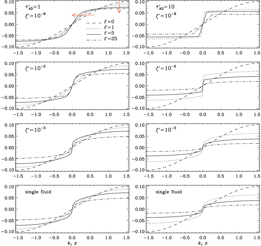
Figure 1: Magnetic field profiles for $\tau_{\rm AD}^{\prime}=1$ (left) and $\tau_{\rm AD}^{\prime}=10$ (right) with $\zeta^{\prime}=10^{-9}$ (top), $\zeta^{\prime}=10^{-5}$ (second row), $\zeta^{\prime}=10^{-3}$ (third row), compared with magnetic field profile in the single fluid model (bottom). The red arrows indicate the temporal evolution.

3.1.1 Formation of sharp structures in one dimension

We examine here a two-fluid model similar to that of Brandenburg & Zweibel (1995) to demonstrates the similarity with the corresponding single fluid model. As initial conditions, we choose for the magnetic field $\bm{B}=(0,\,B_{0}\sin k_{1}x,\,0)$. The $x$ component of the Lorentz force, $\partial B_{y}^{2}/2\partial x$ in this one-dimensional model, drives the charged fluid toward the magnetic nulls at $x=0$ and $\pm\pi$. If the resulting electron pressure gradient remains small enough, this can lead to the formation of sharp structures. In Fig. 1, we compare the results for three values of $\zeta^{\prime}$ and two values of $\rho_{\rm i0}/\rho_{0}$ ($10^{-3}$ and $10^{-4}$) using $\gamma^{\prime}=10^{3}$. The two values of $\rho_{\rm i0}$ correspond to $\tau_{\rm AD}^{\prime}=1$ and $10$, respectively. In all cases, we use $\alpha=\zeta\rho/\rho_{\rm i}^{2}$ to achieve initial ionization equilibrium. We choose $\mbox{\rm Pr}_{\rm M}=20$, but used for $\eta k_{1}/c_{\rm s}$ different values: $10^{-4}$ for $\tau_{\rm AD}^{\prime}=1$ and $2\times 10^{-4}$ for $\tau_{\rm AD}^{\prime}=10$, while in all single fluid models we use $\eta k_{1}/c_{\rm s}=5\times 10^{-5}$. We have increased $\nu$ and $\eta$ to avoid excessive sharpening of the structures in our one-dimensional models. We compare with the results from the one-fluid model in the last two panels of Fig. 1. We also compare models with $\tau_{\rm AD}^{\prime}=1$ and $10$.

We see that for $\zeta^{\prime}=10^{-3}$, good agreement between is the one-fluid and two-fluid models is obtained. The corresponding values of $\alpha$ for ionization equilibrium are $10^{3}$ and $10^{5}$ for $\tau_{\rm AD}^{\prime}=1$ and 10, respectively. This encourages us to examines this model now in three dimensions.

3.1.2 Spectral properties in three dimensions

Next, we consider a setup similar to that studied below in more detail in the one-fluid model. Again, we consider the cases with $\tau_{\rm AD}^{\prime}=1$ and $10$, using $\zeta^{\prime}=10^{-3}$, which was found to give good agreement with the one-fluid model (cf. Fig. 1). We consider here the case of relatively small magnetic diffusivity ($\eta k_{1}/c_{\rm s}=5\times 10^{-5}$), which will also be used in the one-fluid models discussed below.

For both values of $\tau_{\rm AD}$, there is dynamo action with initial exponential growth and subsequent saturation. The mean instantaneous growth rate of the magnetic field, evaluated by averaging $\lambda={\rm d}{}B_{\rm rms}/{\rm d}{}t$ over the duration of the early exponential growth phase, is $\lambda/(c_{\rm s}k_{1})=0.019$. In units of the turnover time, we have $\lambda/(u_{\rm rms0}k_{\rm f}^{\rm eff})=0.080$. For larger values of $\tau_{\rm AD}$, the dynamo saturates at a lower magnetic field strength; see Fig. 2. Running the simulation beyond the early saturation shown here is numerically expensive and would require higher resolution. This is because of sharp gradients in the magnetic field. This problem can be mitigated by increasing the viscosity of the ionized fluid and certainly also by using a larger magnetic diffusivity, which was also used in the one-dimensional runs shown in Fig. 1. The dynamo would then become weaker, however, and this would no longer be the model we would like to study in the one-fluid approximation below.

In Fig. 3, we compare magnetic and kinetic energy spectra for the two values of $\tau_{\rm AD}$. They are normalized such that

$$\int E_{\rm K}(k)\,{\rm d}{}k=\rho_{0}\langle\bm{u}^{2}\rangle/2,\quad\int E_{\rm M}(k)\,{\rm d}{}k=\langle\bm{B}^{2}\rangle/2\mu_{0}.$$ (20)

Here, the kinetic energy is based on the neutral component, but we also consider the kinetic energy of the ionized components, which we normalize by the same density factor,

$$\int E_{\rm i}(k)\,{\rm d}{}k=\rho_{0}\langle\bm{u}_{\rm i}^{2}\rangle/2.$$ (21)

This normalization has the advantage that we can more clearly see that both velocity components are about equally big at large scales (small $k$), when all spectra are also normalized by the same value, namely the total kinetic energy of the neutrals, ${\cal E}_{0}=\rho_{0}u_{\rm rms}^{2}/2$.

We see that there is a marked separation between the ionized and neutral fluid components for larger wavenumbers. The wavenumber above which the two spectra diverge from each other is independent of the value of $\tau_{\rm AD}$, and it is therefore also independent of $k_{\rm AD}$, whose values are indicated by an arrow on the lower abscissa of Fig. 3. There is, however, a strikingly accurate agreement between the viscous dissipation wavenumber, $k_{\nu}$, and the wavenumber where $E_{\rm K}(k)$ and $E_{\rm i}(k)$ begin to diverge from each other. It therefore appears that the value of $k_{\rm AD}$ does not play any role in the dynamics of turbulence with AD. This confirms the earlier result of Brandenburg & Subramanian (2000) that the relevant dissipation wavenumber is independent of AD and is just given by the usual resistive wavenumber $k_{\eta}$, which was defined in Sect. 2.4 and agrees with the wavenumber defined by Xu & Lazarian (2016) after replacing $\epsilon_{\rm M}$ by $k_{\rm f}v_{\rm A}^{3}$.

We also see that the ionized fluid is not efficiently being dissipated at the highest wavenumbers in this model: the kinetic energy spectrum of the ionized fluid does not fall off as much as for the neutral fluid. This is partially explained by the very low ion density in our model, so the actual kinetic energy in the ionized fluid is still not very large. Thus, the energy dissipation may appear insufficient because the amount of energy to be dissipated is very small.

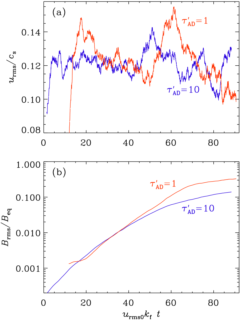
Figure 2: (a) Evolution of the rms velocity (normalized by the sound speed) for the runs with $\tau_{\rm AD}^{\prime}=1$ (red) and $10$ (blue). (b) Evolution of the rms magnetic field for the same runs.

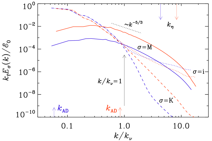
Figure 3: Kinetic energy spectra for the neutral (dashed lines) and ionized fluids (dotted lines) as well as magnetic energy spectra (solid lines) for $\tau_{\rm AD}^{\prime}=1$ (red) and $10$ (blue). The $k^{-5/3}$ slope is shown for orientation.

To understand why the magnetic field is apparently not visibly affected by the breakdown of the strong coupling of the ionized and neutral species below the viscous scale, we have to realize that for $\mbox{\rm Pr}_{\rm M}=20\gg 1$, the velocity at $k\gg k_{\nu}$ is being driven entirely by the magnetic field. Owing to the fact that $\rho_{\rm i}/\rho$ is very small ($10^{-3}$ and $10^{-4}$ for $\tau_{\rm AD}^{\prime}=1$ and $10$, respectively), the velocity is too small to affect the magnetic field. Instead, the magnetic field at large $k$ receives energy only from the magnetic field at larger scales through a forward cascade. This is also evidenced by the fact that, except for a vertical shift, the magnetic spectrum looks similar for $\tau_{\rm AD}^{\prime}=1$ and $10$. This shows that the breakdown of the tight coupling below the resistive scale will not affect our conclusions based on the single fluid approximation considered in the main part of this paper.

3.1.3 Conclusions from the two-fluid model

We have seen that in the two-fluid model, the ionized and neutral components are tightly coupled at large length scales ($k\ll k_{\nu}$). At small scales, however, we see major departures between the two fluids. There are clear differences in the results for the two values of $\tau_{\rm AD}$ studied above. For the larger value of $\tau_{\rm AD}$, the magnetic energy saturates at a smaller value. The magnetic field can therefore no longer drive turbulent motions beyond the viscous cutoff scale, where $E_{\rm K}(k)$ would normally fall off sharply when there is no magnetic field. For the ionized component, on the other hand, the difference between the two spectra is much smaller and a comparatively high fraction of kinetic energy still exists in the ionized component. This is probably indicative of a significant fraction of small-scale magnetic field structures where the ionized and neutral components are counter-streaming in a way similar to what is seen in Fig. 1. After these preliminary studies, we now proceed with the examination of the one-fluid model, which is simpler, but shows similar characteristics and dependencies on $\tau_{\rm AD}^{\prime}$, as we will see.

3.2 The dynamo in one-fluid models

3.2.1 Kinematic evolution

Turning now to the study of dynamo action in the one-fluid model, we first look at the evolution of the rms velocity and magnetic field versus time; see Fig. 4. The magnetic Reynolds numbers of the runs are 1200 for series I and 790 for series II. This lower value for series II is caused by the ten times larger viscosity in this case ($\nu/c_{\rm s}k_{1}=10^{-2}$ instead of $10^{-3}$). We clearly see exponential growth in both cases. The mean instantaneous growth rates are given by $\lambda/(c_{\rm s}k_{1})=0.019$ and $0.010$ for series I and II, respectively. In units of the turnover time, we have $\lambda/(u_{\rm rms0}k_{\rm f}^{\rm eff})=0.080$ and $0.062$ for series I and II, respectively. These values are compatible with the relation $\lambda_{0}\mbox{\rm Re}_{\rm M0}^{1/2}$ with $\lambda_{0}\approx 0.0023$; see also Fig. 3 of Haugen et al. (2004) as well as Fig. 3 of Brandenburg (2009), were similar values of $\mbox{\rm Re}_{\rm M0}\approx 1000$ were found and the $\mbox{\rm Re}_{\rm M0}^{1/2}$ scaling was demonstrated.

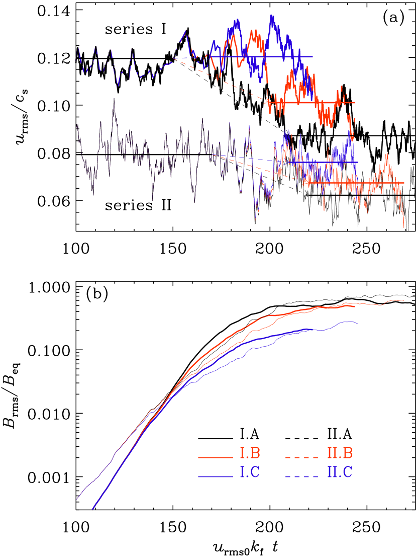
Figure 4: (a) Evolution of the rms velocity (normalized by the sound speed) for each of the three runs of series I and II. The values of late time averages are indicated by horizontal lines in the corresponding color and connected by dashed arrows to the corresponding horizontal line for the kinematic stage. (b) Evolution of the rms magnetic field for series I (solid lines) and II (dashed lines) for small (black lines for runs I.A and II.A), intermediate (red lines for I.B and II.B), and large values (blue lines for I.C and II.C) of $\mbox{\rm St}_{\rm AD}$.

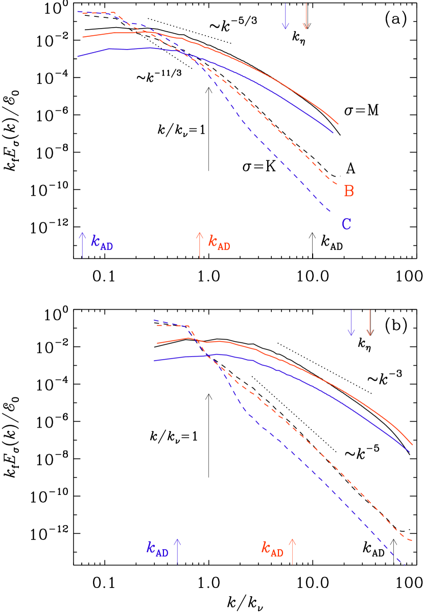
Figure 5: Spectra of magnetic ($i={\rm M}$, solid lines) and kinetic ($i={\rm K}$, dashed lines) for each of the three runs in series I (top) and II (bottom).

For all runs, the magnetic field eventually saturates owing to the nonlinearity of the problem. In addition to the Lorentz force, $\bm{J}\times\bm{B}$, there is the AD nonlinearity. It is a priori unclear which of the two is more important. The saturation phenomenology of the small-scale dynamo has been studied by Cho et al. (2009). Xu & Lazarian (2016) found that this dynamo saturation is independent of plasma effects including AD. Interestingly, Fig. 4 now shows that for $\mbox{\rm St}_{\rm AD}\geq 1$, the AD nonlinearity does affect the solution, and this happens already when $B_{\rm rms}/B_{\rm eq}\geq 0.02$. We also see that the kinetic energy decreases only very little during saturation when AD is strong (cf. cases I.C and II.C). This is because the velocity is only affected by the magnetic field, whose saturation levels diminish with increasing values of $\mbox{\rm St}_{\rm AD}$.

3.2.2 Spectral properties

Next, we consider kinetic and magnetic energy spectra for series I and II, $E_{\rm K}(k,t)$ and $E_{\rm M}(k,t)$, respectively. For both series, the kinetic energy spectra are found to be unaffected for $k<k_{\nu}$, while the magnetic energy is clearly suppressed by AD at all wavenumbers. The magnetic energy spectrum does not really show power law scaling, but it has a slope compatible with $k^{-5/3}$, although the spectrum tends to become slightly shallower at high wavenumbers when AD is strong (compare the red and blue lines in Fig. 5 with the black ones). This could be a signature of sharp structures that are expected to develop in the presence of AD (Brandenburg & Zweibel, 1994; Zweibel & Brandenburg, 1997). Sharp structures could be responsible for producing enhanced power at high wavenumbers. This is an effect that was also seen in the turbulence simulations of Brandenburg & Subramanian (2000).

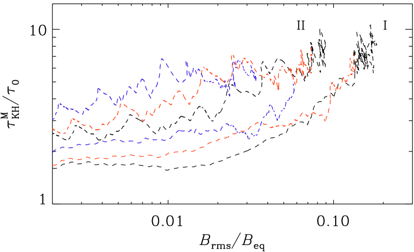
Figure 6: Magnetic Kelvin-Helmholtz time normalized by the turnover time versus normalized magnetic field strength.

In both series I and II, the kinetic energy spectrum develops a clear power law in the dissipation range, especially for series II, where power law scaling extends over about 1.5 decades, while for series I, the same power law is seen for only about half a decade. The power law scaling of $E_{\rm K}(k)$ is solely a consequence of magnetic driving at $k>k_{\nu}$ when $\mbox{\rm Pr}_{\rm M}$ is large.

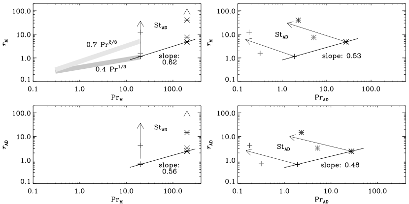
Figure 7: Ratio of kinetic to magnetic and kinetic to ambipolar dissipation rates versus magnetic and ambipolar Prandtl numbers. The light and darker gray lines denote the scaling found by Brandenburg (2014) for large- and small-scale dynamos, respectively.

Also the magnetic energy spectrum shows a range with power law scaling for series II, where $E_{\rm M}\propto k^{-5/3}$. For series I the $k^{-5/3}$ scaling is not so clear. The kinetic energy spectrum is much steeper and has a slope comparable with a $k^{-11/3}$ spectrum. This is reminiscent of the Golitsyn spectrum of magnetic energy, which applies to the opposite case of small magnetic Reynolds numbers (Golitsyn, 1960). In that case, the electromotive force is balanced by the magnetic diffusion term rather than the time derivative of $\bm{B}$. The similarity suggests that in the present case, the velocity is driven through the balance between the Lorentz force and the viscous force (which is proportional to $\nu\nabla^{2}\bm{u}$) rather than through a balance with the ${\rm D}{}\bm{u}/{\rm D}{}t$ inertial term.

The magnetic energy spectrum peaks at a wavenumber $k_{\ast}$ that can roughly be estimated by Subramanian’s formula $k\ast\approx k_{\rm f}\mbox{\rm Re}_{\rm M,c}^{1/2}$ (Subramanian, 1999). Estimating $\mbox{\rm Re}_{\rm M,c}\approx 40$ for the critical magnetic Reynolds number for dynamo action (Haugen et al., 2004), we have $k_{\ast}/k_{\nu}\approx 0.5$ and $2.8$ for series I and II, respectively. This is in fair agreement with the position of the magnetic peak wavenumber seen in Fig. 5. Schober et al. (2015) proposed a revised estimate with an exponent $3/4$ for Kolmogorov turbulence and a larger prefactor, so the corresponding values are by about a factor of eight larger. I addition, both estimates would yield bigger values if $2\pi$ factors in their definitions of $\mbox{\rm Re}_{\rm M}$ were taken into account.

3.2.3 Comment on numerical diffusion

At this point, a comment on the accuracy and properties of the numerical scheme is in order. The results presented above relating to the spectral kinetic energy scaling in the high magnetic Prandtl number regime rely heavily upon the presence of proper diffusion operators. In fact, those are the only terms balancing an otherwise catastrophic steepening of gradients by the $\bm{u}\cdot{\bm{\nabla}}\bm{u}$, $\bm{u}\times\bm{B}$, and $\bm{J}\times\bm{B}$ nonlinearities. The weakly stabilizing properties of any third order time stepping scheme and the dispersive errors of the spatial derivative operators such as $\bm{u}\cdot{\bm{\nabla}}$ do not contribute noticeably to numerical diffusion below wavenumbers of half the Nyquist wavenumber (Brandenburg, 2003), which is the largest wavenumber shown in our spectra. This is different from codes that solve the ideal hydromagnetic equations. Those codes prevent excessive steepening of gradients by the numerical scheme in ways that cannot be quantified by an actual viscosity or diffusivity. This is sometimes also called numerical diffusion, but such a procedure it is not invoked in the numerical simulations presented here.

3.2.4 Magnetic dissipation

If the magnetic field were not constantly regenerated by dynamo action, it would decay on a timescale that we call the magnetic Kelvin-Helmholtz time,

$$\tau_{\rm KH}^{\rm M}={\cal E}_{\rm M}/\epsilon_{\rm M}.$$ (22)

In Fig. 6, we plot its instantaneous value versus the instantaneous magnetic field strength as the dynamo saturates and the field strength thus increases. Almost independently of the presence or absence of AD and regardless of whether we consider series I or II, the ratio $\tau_{\rm KH}^{\rm M}/\tau_{0}$ is always around eight; see the two concentrations of data near $B_{\rm rms}/B_{\rm eq}\approx 0.08$ and $0.16$ for series I and II, respectively.

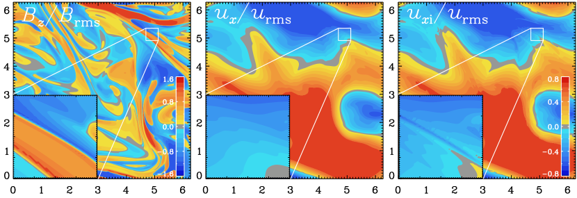
Figure 8: Visualizations of $B_{z}/B_{\rm rms}$, $u_{x}/u_{\rm rms}$, and $u_{x{\rm i}}/u_{\rm rms}$ for the two-fluid model with $\mbox{\rm St}_{\rm AD}=0.15$ or $\tau_{\rm AD}^{\prime}=1$. The insets show a blow-up near a magnetic structure.

In the absence of AD, it was found that the ratio $r_{\rm M}=\epsilon_{\rm M}/\epsilon_{\rm K}$ of magnetic to kinetic energy dissipation increases with increasing values of $\mbox{\rm Pr}_{\rm M}$ like $\mbox{\rm Pr}_{\rm M}^{1/3}$ for small-scale dynamo action and like $\mbox{\rm Pr}_{\rm M}^{2/3}$ for large-scale dynamo action (in the presence of kinetic helicity of the turbulent flow). In the presence of AD, there is an additional mode of dissipation proportional to $\epsilon_{\rm AD}$. On the other hand, also the effective magnetic Prandtl number is modified if we include $\eta_{\rm AD}$ in the definition of $\mbox{\rm Pr}_{\rm M}$, as in Equation (17). The question is therefore whether there is any analogy between Ohmic dissipation and dissipation through AD. To assess this, we plot in Fig. 7 all four possibilities: $r_{\rm M}$ versus $\mbox{\rm Pr}_{\rm M}$ and $\mbox{\rm Pr}_{\rm AD}$, as well as $r_{\rm AD}$ versus $\mbox{\rm Pr}_{\rm M}$ and $\mbox{\rm Pr}_{\rm AD}$.

Both $r_{\rm M}$ and $r_{\rm AD}$ are seen to increase with $\mbox{\rm St}_{\rm AD}$, so the data points generally move upward in all four plots. However, as we increase $\mbox{\rm St}_{\rm AD}$, we also decrease $\mbox{\rm Pr}_{\rm AD}$, so the data points move to the left in Fig. 7. In this sense, there is no analogy with Ohmic dissipation. It should be noted, of course, that both Ohmic dissipation and AD are no longer accurate descriptions of the physics on small length scales. It would therefore be interesting to revisit this question when such an analysis of the full kinetic equations becomes feasible; see Rincon et al. (2016) and Zhdankin et al. (2017) for relevant references. It is worth noting in this connection that the case with $\mbox{\rm Pr}_{\rm M}\gg 1$ is special because the work done against the Lorentz force, which quantifies the conversion of kinetic to magnetic energy, only operates on large length scales when $\mbox{\rm Pr}_{\rm M}\gg 1$. At small length scales, the sign of this term is reversed, so Brandenburg & Rempel (2019) called this reversed dynamo action. This means that the magnetic energy is not ohmically dissipated at small length scales, but viscously. Brandenburg & Rempel (2019) speculated further that this loss of energy would really correspond to the energization of ions and electrons, although there is currently no evidence that this similarity is quantitatively accurate.

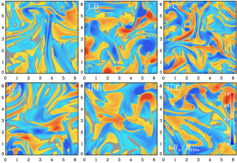
Figure 9: Visualizations of $B_{z}(x,y)/B_{\rm rms}$ for the single fluid models, Runs I.A–C and II.A–C.

Table 1: Summary of the runs discussed in the paper.

Run $\mbox{\rm Re}_{\rm M}$ $\mbox{\rm Pr}_{\rm M}\!\!$ $\mbox{\rm Pr}_{\rm AD}$ $r_{\rm M}$ $r_{\rm AD}$ $\mbox{\rm St}_{\rm AD}$ $\!\!\langle E^{2}\rangle/\langle B^{2}\rangle\!\!$ $\mbox{skew}\,E$ $\mbox{skew}\,B$ $\mbox{kurt}\,E$ $\mbox{kurt}\,B$ $\mbox{kurt}\,\bm{B}$ I.a 800 20 18.3 0.84 0.79 0.00012 $1.66$ $2.05$ $0.19$ $14.9$ $3.38$ 2.33 I.b 840 20 15.7 0.86 0.73 0.00039 $1.80$ $2.00$ $-0.36$ $11.7$ $3.60$ 1.92 I.c 850 20 10.5 0.97 0.71 0.00130 $1.60$ $1.32$ $0.04$ $4.58$ $1.20$ 1.35 I.d 830 20 5.15 1.15 0.72 0.0038 $1.41$ $0.97$ $-0.05$ $4.99$ $2.57$ 0.66 I.A 860 20 1.9 1.15 0.65 0.013 $1.46$ $0.85$ $0.01$ $6.30$ $3.73$ 0.08 I.e 800 20 0.71 1.25 0.65 0.037 $1.33$ $0.41$ $0.17$ $5.34$ $3.21$ $-0.06$ I.B 1000 20 0.32 1.58 0.70 0.15 $1.21$ $-0.18$ $0.02$ $1.77$ $1.08$ $-0.43$ I.C 1170 20 0.18 12.3 4.12 1.79 $1.12$ $-0.27$ $0.05$ $2.08$ $1.18$ $-0.57$ II.A 630 200 27.4 4.79 2.35 0.010 $1.27$ $0.72$ $-0.13$ $2.17$ $1.32$ 3.19 II.B 670 200 5.13 7.42 3.20 0.10 $1.43$ $0.06$ $-0.08$ $0.91$ $1.75$ 2.50 II.C 770 200 2.31 40.0 14.6 1.19 $1.29$ $-0.48$ $-0.04$ $3.71$ $1.71$ 2.48

3.3 Spatial features related to AD

3.3.1 Visual inspection

In Fig. 8, we show $xy$ slices of $B_{z}/B_{\rm rms}$ and compare with slices of the $x$ component of the neutral and ionized flows, $u_{x}/u_{\rm rms}$ and $u_{x{\rm i}}/u_{\rm rms}$, respectively, in the same (arbitrarily chosen) plane. The magnetic field displays folded structures in places, as was first emphasized by Schekochihin et al. (2004), but Brandenburg and Subramanian (2005) found that there are also many other places in the volume that are not strongly folded. Some of the folds lead to differences between the neutral and ionized fluid components; see the insets of Fig. 8. In most other places, however, the two velocity species are remarkably similar. The $y$ and $z$ components of $\bm{u}$ and $\bm{u}_{\rm i}$ are also similar to each other and show only small differences near magnetic structures.

Next, we compare the magnetic field for different one-fluid models; see Fig. 9, where we compare the three models of series I and II. The overall magnetic field strength is weaker for model C compared with models B and A. To remove this aspect from the comparison, we plot in Fig. 9 the $B_{z}$ components of the magnetic field normalized by the rms values for each model.

It is hard to see systematic differences between the different cases. There could be more locations with strong horizontal gradients in $B_{z}(x,y)$, where $\mbox{\rm St}_{\rm AD}$ is large (compare Runs C of series I and II with Runs A and B of the corresponding series), but the resulting changes are not very obvious. There are also no clear differences between series I and II themselves. For these reasons, it is important to look at statistical measures to study the differences. This will be done next.

3.3.2 Statistical analysis

In this section, we investigate in more quantitative detail the effects of AD on the structure of the magnetic field. We know that AD tends to clip the peaks of the magnetic field at locations where its strength is large (Brandenburg & Zweibel, 1995). This should lead to a reduced kurtosis,

$$\mbox{kurt}\,B_{i}=\langle B_{i}^{4}\rangle/\langle B_{i}^{2}\rangle^{2}-3.$$ (23)

It is unclear, however, whether this is a statistically significant effect. To examine this, we compute the resulting values of $\mbox{kurt}(B_{i})$. Since our simulations are isotropic, we can improve the statistics of the kurtosis by taking the average over all three directions, i.e., we define $\mbox{kurt}\,\bm{B}$ (bold without subscript on $\bm{B}$) as

$$\mbox{kurt}\,\bm{B}=(\mbox{kurt}\,B_{x}+\mbox{kurt}\,B_{y}+\mbox{kurt}\,B_{z})/3,$$ (24)

and compute it for each of the two series and for different values of $\mbox{\rm St}_{\rm AD}$. In this context, we recall that the kurtosis vanishes for gaussian-distributed data, and it is 3 for an exponential distribution. Here we find a systematic crossover from values somewhat smaller than 3 to negative values when $\mbox{\rm St}_{\rm AD}\mathrel{\mathchoice{\vbox{\offinterlineskip\halign{\hfil$\displaystyle#$\hfil\cr>\cr\sim\cr}}}{\vbox{\offinterlineskip\halign{\hfil$\textstyle#$\hfil\cr>\cr\sim\cr}}}{\vbox{\offinterlineskip\halign{\hfil$\scriptstyle#$\hfil\cr>\cr\sim\cr}}}{\vbox{\offinterlineskip\halign{\hfil$\scriptscriptstyle#$\hfil\cr>\cr\sim\cr}}}}0.02$; see Fig. 10 for series I and II with $\mbox{\rm Pr}_{\rm M}=20$ and $200$, respectively. Here we have included the additional runs I.a–e with lower values $\mbox{\rm St}_{\rm AD}$ have been added. This dependence can roughly be described by a fit of the form

$$\ln\mbox{kurt}\,\bm{B}=e^{\kappa_{\infty}}+\mbox{\rm St}_{\rm AD}^{-\alpha},$$ (25)

where $\kappa_{\infty}\approx 2.36$ is the value of $\mbox{kurt}\,\bm{B}+3$ for large values of $\mbox{\rm St}_{\rm AD}$ and $\alpha\approx 0.61$ is the slope for smaller values. Additional terms and parameters could be included in this fit to account for finite values of the kurtosis for $\mbox{\rm St}_{\rm AD}\to 0$, but this does not appear to be necessary for describing the present data; see Table LABEL:Tsummary. In conclusion, it appears that the measurement of the kurtosis of the magnetic field in the interstellar medium could be a useful diagnostic tool that should be explored further in future.

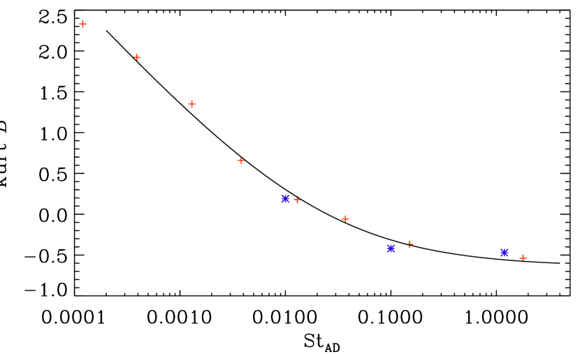
Figure 10: Dependence of $\mbox{kurt}\,\bm{B}$ on $\mbox{\rm St}_{\rm AD}$. The red (blue) symbols denote the results for series I (II).

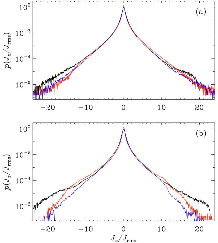
Figure 11: Histograms of $J_{z}$ for (a) series I and (b) series II. Black, red, and blue lines denote the cases A, B, and C, respectively.

In Fig. 11 we show histograms of $J_{z}$ for series I and II. We see that, as $\mbox{\rm St}_{\rm AD}$ is increased, the wings of the distributions are being clipped slightly. On the other hand, the amount of clipping is actually relatively small compared with the increase in magnetic field strength as $\mbox{\rm St}_{\rm AD}$ is increased. This is to be expected, because AD tends to create force-free regions where $(\bm{J}\times\bm{B})^{2}$ is minimized and $(\bm{J}\cdot\bm{B})^{2}$ is maximized. In between those regions, on the other hand, there are sharp current sheets that were already found in the earlier work of Brandenburg & Zweibel (1994).

It is important to note that one usually never measures the magnetic field directly, but instead the linear polarization through either synchrotron radiation or through dust emission. In both cases, it therefore appears useful to discuss the two rotationally invariant modes of linear polarization, namely the $E$ and $B$ mode polarizations. This will be done in the next section.

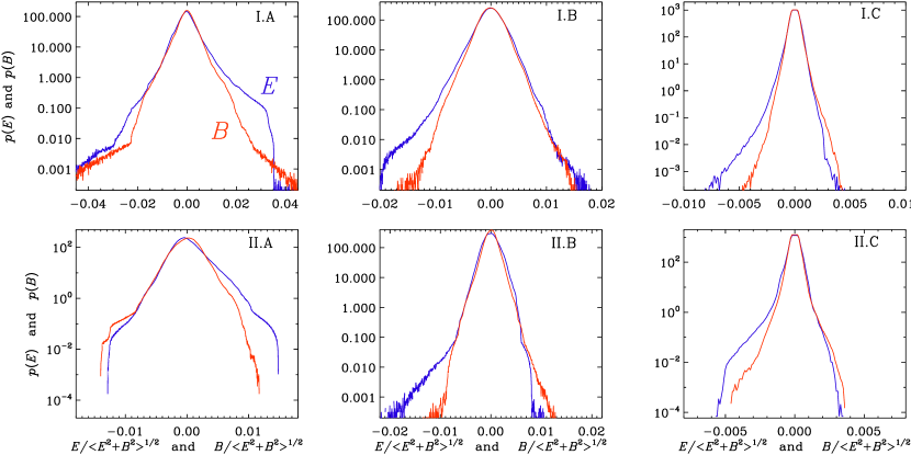
Figure 12: $E$ and $B$ mode polarizations for series I (upper row) and II (lower row). Blue (red) lines denote the normalized probability density functions of $E$ ($B$) mode polarization.

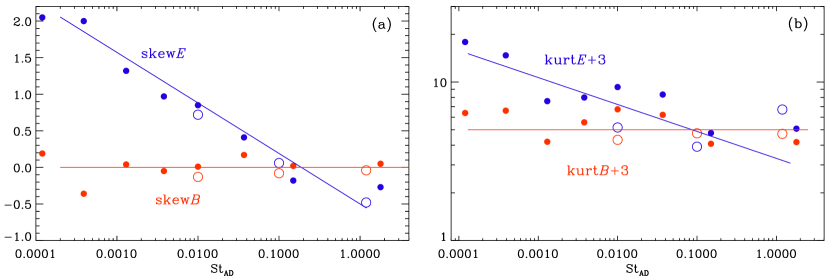
Figure 13: (a) Dependence of $\mbox{skew}\,E$ (blue) and $\mbox{skew}\,B$ (red) on $\mbox{\rm St}_{\rm AD}$ and (b) dependence of $\mbox{kurt}\,E+3$ (blue) and $\mbox{kurt}\,B+3$ (red) on $\mbox{\rm St}_{\rm AD}$. Filled (open) symbols refer to series I (II). The straight lines represent approximate fits given by $\mbox{skew}\,E=-0.5-0.3\ln\mbox{\rm St}_{\rm AD}$ (blue) and $\mbox{skew}\,B=0$ (red) in (a), and $\mbox{kurt}\,E+3=3.3\,\mbox{\rm St}_{\rm AD}^{0.17}$ (blue) and $\mbox{kurt}\,B=2$ (red) in (b).

3.4 $E$ and $B$ mode polarizations

The analysis of $E$ and $B$ mode polarization has been particularly important in the context of cosmology (Kamionkowski et al., 1997; Seljak & Zaldarriaga, 1997) and, more recently, in the context of dust foreground polarization (Planck Collaboration Int. XXX, 2016). It was found that there is a systematic excess of $E$ mode power over $B$ mode power by about a factor of two, which was unexpected at the time (Caldwell et al., 2017). Different proposals exist for the interpretation of this. It is possible that the excess of $E$ mode polarization is primarily an effect of the dominance of the magnetic field, i.e., a result of magnetically over kinetically dominated turbulence (Kandel et al., 2017). Using simulations of supersonic hydromagnetic turbulent star formation, Kritsuk et al. (2018) found that the observed $E$ over $B$ ratio can be reproduced. However, not enough work has been done to assess the full range of possibilities for different types of flows. For solar linear polarization, for example, it has been found that there is no excess of $E$ over $B$ mode polarization, although the possibility of instrumental effects has not yet been conclusively addressed (Brandenburg et al., 2019).

Looking at Fig. 12, we see that, as $\mbox{\rm St}_{\rm AD}$ is increased, there is a systematic change of the skewness of $E$ (but not of $B$) as $\mbox{\rm St}_{\rm AD}$ is increased. For small values of $\mbox{\rm St}_{\rm AD}$, the skewness is positive and for large values it is negative. Here we define the skewness as

$${\rm skew}E=\langle E^{3}\rangle/\sigma_{E}^{3},\quad{\rm skew}B=\langle B^{3}\rangle/\sigma_{B}^{3},$$ (26)

where $\sigma_{E}^{2}=\langle E^{2}\rangle-\langle E\rangle^{2}$ and $\sigma_{B}^{2}=\langle B^{2}\rangle-\langle B\rangle^{2}$ are their variances. Note that here the $B$ is not to be confused with the components $B_{i}$ of the magnetic field, which are related to each other only through Equation (18).

The increase of the skewness of $E$ with $\mbox{\rm St}_{\rm AD}$ is seen both for series I (where $\mbox{skew}\,E=-0.27$ for $\mbox{\rm St}_{\rm AD}\approx 1.8$ in I.C) and series II (where $\mbox{skew}\,E=-0.48$ for $\mbox{\rm St}_{\rm AD}\approx 1.2$ in II.C). For small values of $\mbox{\rm St}_{\rm AD}$, however, there is a much more dramatic effect in that $\mbox{skew}\,E$ reaches values of around $2$, which is much more extreme than what was found earlier for decaying hydromagnetic turbulence. Even a change of $\mbox{\rm St}_{\rm AD}$ from $10^{-2}$ (I.A) to $10^{-4}$ (II.a), has a strong effect in that skew changes from 0.85 to 2. The kurtosis of $E$ reaches more extreme values much larger than 10; see Fig. LABEL:Tsummary for a summary of the statistics of $E$ and $B$. Although we have not determined error bars, we can get a sense of the reliability of the data by noting that the trend with $\mbox{\rm St}_{\rm AD}$ is reasonably systematic; see Fig. 13.

In view of the negative skewness found previously for decaying hydromagnetic turbulence (Brandenburg et al., 2019), it now appears that negative skewness of $E$ is not a general property of hydromagnetic turbulence, although it may well appear in the interstellar medium where both AD can be present and magnetic fields can be significant. AD can also play a role in the solar chromosphere, where it contributes to heating cold pockets of gas (Khomenko & Collados, 2017). It needs to be checked whether this can lead to observable effects. The analysis of $E$ and $B$ mode polarization is therefore, an interesting diagnostic tool, although more work needs to be done to learn about all the possible ways of interpreting those two modes of polarization.

4 Conclusions

In the cold interstellar medium, ionization and recombination are important. The electron pressure can then be neglected and the single fluid approach of AD becomes an excellent approximation. Our work has now demonstrated that AD does not have diffusive properties in the sense of enhancing the effects of microphysical magnetic diffusion. This is most likely due to the fact that AD is a nonlinear effect that operates only in places where the field is strong in the sense that $\tau_{\rm AD}v_{\rm A}^{2}\gg\tau_{0}u_{\rm rms}^{2}$. In fact, in one dimension it is easy to see that the Lorentz force acting on the ionized fluid works in such a way as to move more ionized fluid towards the magnetic null (Brandenburg & Zweibel, 1995). This depletes the field maxima and leads to a pile-up of magnetic field just before the magnetic null. This effect is particularly pronounced when $\tau_{\rm AD}\gg\tau_{0}$, and thus $\mbox{\rm St}_{\rm AD}\gg 1$.

Although the spectral shape at large $k$ is only weakly affected by AD, it does have a clear effect on the kinetic energy spectrum at $k>k_{\nu}$ and suppresses the spectral kinetic energy of the neutrals markedly. The kinetic energy of the charged species is even slightly enhanced. This is surprising, because the overall rms velocity of the neutrals is hardly affected at all. One must keep in mind, however, that not much kinetic energy is contained deep in the kinetic energy tail at large $k$. In fact, the only reason why there is some level of kinetic energy at all is that, owing to the large magnetic Prandtl number, there is still significant magnetic energy at those high wavenumbers that drives the kinetic motions.

From an observational point of view, we can identify two potentially useful ways of diagnosing the importance of AD in the interstellar medium. First, there is the direct effect on the statistics of the magnetic field. The importance of AD can then potentially be quantified by measuring the kurtosis of the components of the magnetic field. Alternatively, there appears to be a systematic effect on the statistics of the $E$ and $B$ mode polarizations. While the $B$ mode polarization is generally unaffected by turbulence, the $E$ mode polarization can exhibit non-vanishing skewness, which is positive for a weak AD and negative for strong AD. This is an unexpected signature in view of recent results for decaying hydromagnetic turbulence, where the skewness was found to be negative even without AD.

In this work, we have studied only two values of the magnetic Prandtl number. However, the effect of changing the value of $\mbox{\rm Pr}_{\rm M}$ on observational properties such as $E$ and $B$ is rather weak; see Fig. 13. This is interesting because in cold molecular clouds, the magnetic Prandtl number can potentially drop below unity. It would therefore in future be useful to study whether the present results carry over into the regime of lower values of $\mbox{\rm Pr}_{\rm M}$ (possibly below unity), and whether the effects on the skewness of $E$ and $B$ mode polarizations remain unchanged.

$Header: /var/cvs/brandenb/tex/mhd/AD/paper.tex,v 1.98 2019/05/29 02:30:00 brandenb Exp $

References

- Brandenburg (2003) Brandenburg, A. 2003, in Advances in nonlinear dynamos (The Fluid Mechanics of Astrophysics and Geophysics, Vol. 9), ed. A. Ferriz-Mas & M. Núñez (Taylor & Francis, London and New York), 269
- Brandenburg (2009) Brandenburg, A. 2009, ApJ, 697, 1206
- Brandenburg (2014) Brandenburg, A. 2014, ApJ, 791, 12
- Brandenburg & Rempel (2019) Brandenburg, A., & Rempel, M. 2019, ApJ, in press, arXiv:1903.11869
- Brandenburg & Subramanian (2000) Brandenburg, A., & Subramanian, K. 2000, A&A, 361, L33
- Brandenburg and Subramanian (2005) Brandenburg, A., & Subramanian, K. 2005, Phys. Rep., 417, 1
- Brandenburg & Zweibel (1994) Brandenburg, A., & Zweibel, E. G. 1994, ApJ, 427, L91
- Brandenburg & Zweibel (1995) Brandenburg, A., & Zweibel, E. G. 1995, ApJ, 448, 734
- Brandenburg et al. (2019) Brandenburg, A., Bracco, A., Kahniashvili, T., Mandal, S., Roper Pol, A., Petrie, G. J. D., & Singh, N. K. 2019, ApJ, 870, 87
- Brandenburg et al. (2018) Brandenburg, A., Haugen, N. E. L., Li, X.-Y., & Subramanian, K. 2018, MNRAS, 479, 2827
- Caldwell et al. (2017) Caldwell, R. R., Hirata, C., & Kamionkowski, M. 2017, ApJ, 839, 91
- Cho et al. (2009) Cho, J., Vishniac, E. T., Beresnyak, A., Lazarian, A., & Ryu, D. 2009, ApJ, 693, 1449
- Draine (1986) Draine, B. T. 1986, MNRAS, 220, 133
- Draine et al. (1983) Draine, B. T., Roberge, W. G., & Dalgarno, A. 1983, ApJ, 264, 485
- Golitsyn (1960) Golitsyn, G. S. 1960, Sov. Phys. Dokl., 5, 536
- Haugen et al. (2004) Haugen, N. E. L., Brandenburg, A., & Dobler, W. 2004, Phys. Rev. E, 70, 016308
- Kamionkowski et al. (1997) Kamionkowski, M., Kosowsky, A., & Stebbins, A. 1997, Phys. Rev. Lett., 78, 2058
- Kandel et al. (2017) Kandel, D., Lazarian, A., & Pogosyan, D. 2017, MNRAS, 472, L10
- Khomenko & Collados (2017) Khomenko, E., & Collados, M. 2012, ApJ, 747, 87
- Kritsuk et al. (2018) Kritsuk, A. G., Flauger, R., & Ustyugov, S. D. 2018, Phys. Rev. Lett., 121, 021104
- McCall et al. (2003) McCall, B. J., Huneycutt, A. J., Saykally, R. J., Geballe, T. R., Djuric, N., Dunn, G. H., Semaniak, J., Novotny, O., Al-Khalili, A., Ehlerding, A., Hellberg, F., Kalhori, S., Neau, A., Thomas, R., Österdahl, F., & Larsson, M. 2003, Nature, 422, 500
- McKee et al. (1993) McKee, C. F., Zweibel, E. G., Goodman, A. A., & Heiles, C. 1993, in Protostars and Planets III, ed. E. H. Levy, L. J. Lunine & M. S. Mathews (University of Arizona Press, Tucson), 327
- Padoan et al. (2000) Padoan, P., Zweibel, E. G., & Nordlund, Å. 2000, ApJ, 540, 332
- Planck Collaboration Int. XXX (2016) Planck Collaboration Int. XXX. 2016, A&A, 586, A133
- Rincon et al. (2016) Rincon, F., Califano, F., Schekochihin, A. A., & Valentini, F. 2016, Proc. Nat. Acad. Sci., 113, 3950
- Schekochihin et al. (2004) Schekochihin, A. A., Cowley, S. C., Taylor, S. F., Maron, J. L., McWilliams, J. C. 2004, ApJ, 612, 276
- Schober et al. (2015) Schober, J., Schleicher, D. R. G., Federrath, C., Bovino, S., & Klessen, R. S. 2015, Phys. Rev. E, 92, 023010
- Seljak & Zaldarriaga (1997) Seljak, U., & Zaldarriaga, M. 1997, Phys. Rev. Lett., 78, 2054
- Subramanian (1999) Subramanian, K. 1999, Phys. Rev. Lett., 83, 2957
- Williamson (1980) Williamson, J. H. 1980, J. Comput. Phys., 35, 48
- Xu & Lazarian (2016) Xu, S., & Lazarian, A. 2016, ApJ, 833, 215
- Xu et al. (2019) Xu, S., Garain, S. K., Balsara, D. S., & Lazarian, A. 2019, ApJ, 872, 62
- Zhdankin et al. (2017) Zhdankin, V., Werner, G. R., Uzdensky, D. A., & Begelman, M. C. 2017, Phys. Rev. Lett., 118, 055103
- Zweibel & Brandenburg (1997) Zweibel, E. G., & Brandenburg, A. 1997, ApJ, 478, 563