Abstract

Time series models such as dynamical systems are frequently fitted to a cohort of data, ignoring variation between individual entities such as patients. In this paper we show how these models can be personalised to an individual level while retaining statistical power, via use of multi-task learning (MTL). To our knowledge this is a novel development of MTL which applies to time series both with and without control inputs. The modelling framework is demonstrated on a physiological drug response problem which results in improved predictive accuracy and uncertainty estimation over existing state-of-the-art models.

1 INTRODUCTION

In this paper we study the response of a patient’s physiology under the effect of drug infusion, specifically the effect of the anaesthetic agent Propofol on vital signs. There is a long history of pharmacokinetic/pharmacodynamic (PK/PD) models used to study such effects (see e.g. Bailey and Haddad, 2005, and Minto and Schnider, 2008). We are particularly interested in the personalisation of such models to individual patients. Our focus here will be the on the personalisation of the pharmacodynamic (PD) model, as this issue has already been addressed for the PK component (see e.g. Eleveld et al., 2018).

We approach this problem as one of multi-task learning (MTL), where each patient is treated as a task. We show that the parameters across patients can be well-modelled as a low-dimensional latent linear subspace. Our results indicate that approximately five such latent variables suffice to describe the inter-patient variation in response we observe in a clinical study, and lead to improved predictive accuracy and uncertainty estimation over existing state-of-the-art models.

The application of MTL to time series models is unusual, especially for individuals unrelated in space and time. In this work we generalise multi-task learning to tasks described by dynamical systems – an important class of time series models. Comparison to existing work is given in Section 4 including the new classes of models to which we extend the MTL framework.

The structure of the paper is as follows: Section 2 provides an overview of the PK/PD model and its personalisation. Section 3 introduces our proposed model; related work is discussed in Section 4. Our results on clinical data are summarised and discussed in Section 5, and some concluding remarks are given in Section 6.

2 PHARMACOKINETIC-PHARMACODYNAMIC (PK/PD) MODELS

PK/PD models are the dominant paradigm for modelling the response to a continuously infused drug. We use the anaesthetic agent Propofol as our running example. These models decompose the problem into two sub-tasks. Of primary interest in the literature is the pharmacokinetic (PK) process, which relates the administration of a drug to its distribution and elimination in the body over time. This provides insight into the evolution of drug concentrations in regions of the body including major blood vessels. A pharmacodynamic (PD) process models the relationship between blood concentration and the effect on observed physiological effects, such as vital signs (e.g. heart rate, blood pressure). Below, we briefly discuss common approaches to these models.

PK models.

The most commonly described PK model in anaesthesia is the three-compartment model. This is an Ordinary Differential Equation (ODE) describing drug concentrations for differently perfused physiological compartments under a continuous time infusion. These compartments notionally correspond to blood, muscle and fat, and can be conceptualised with the latter two as ‘peripheral’ compartments each connected only to the central compartment, blood. The drug in-flow from a Target Controlled Infusion (TCI) pump, $\omega(t)$ enters the central compartment and the concentrations $\mathbf{c}(t)=(c_{1}(t),\,c_{2}(t),\,c_{3}(t))^{\mkern-1.5mu\mathsf{T}}$ of all compartments evolve as:

$$\frac{\operatorname{d\!}\mathbf{c}}{\operatorname{d\!}t}=A\mathbf{c}(t)+\mathbf{e}_{1}\omega(t)$$ (1)

for a given matrix $A$ of rate constants (see supplementary material), and the first ordinate unit vector $\mathbf{e}_{1}$. There is a large body of literature pertaining to the PK model and it exhibits strong performance in experimental and clinical settings. Much work has been done to personalise the rate constants in the matrix $A$ based on patient covariates (see below). It is notable that the rate constants have become part of the vocabulary of practicing anaesthetists.

PD models.

The mechanism by which physiological effects follow from the blood concentration of some drug is not well understood; PD models propose a direct relationship to the concentration at some physiological effect site. The effect site concentration $x(t)$ may not have reached equilibrium with the central compartment concentration $c_{1}(t)$ and can introduce a lag to the observed effect. Denoting the rate constants as $k_{1e}$ for the in-flow to the effect site and $k_{e0}$ for the elimination, the relationship is modelled as:

$$\frac{\operatorname{d\!}x}{\operatorname{d\!}t}=k_{1e}c_{1}(t)-k_{e0}x(t).$$ (2)

For multidimensional observations, independent effect sites $x_{j}(t),j=1,\ldots d$ are usually fitted. For instance, the observation channels in our dataset consist of systolic and diastolic blood pressure (BPsys and BPdia respectively), and the Bispectral Index (BIS). The relationship of the effect site to observations $y_{j}(t),j=1,\ldots d$ are then modelled by some nonlinear transformation plus white noise, i.e. for a given time $t$, $y_{j}(t)=\mathcal{N}(g_{\theta}(x_{j}(t)),\tau^{-1})$. Common choices of $g_{\theta}(\cdot)$ are the Hill function (Hill, 1910) or generalised logistic sigmoid (see e.g. Georgatzis et al. 2016):

$$g_{\theta}(x)=\theta_{1}+\frac{\theta_{2}-\theta_{1}}{(1+\exp\{-\theta_{3}x\})^{1/\theta_{4}}}.$$ (3)

Personalisation.

A number of attempts have been made to personalise PK models using patient attributes such as age, gender, height or weight (see e.g. Marsh et al. 1991; Schnider et al. 1998; White et al. 2008 and Eleveld et al., 2018 for a combined study). Various studies (see e.g. Glen and Servin, 2009; Masui et al., 2010; Glen and White, 2014) have compared the predictive performance of several propofol PK models currently used for target controlled infusion (TCI) in clinical practice. These studies have confirmed a degree of bias and inaccuracy of the models but overall their performance is considered by most clinicians to be adequate for clinical use (at least within the populations in which they were developed).

In most commercially available implementations of the Marsh and Schnider models, fixed $k_{1e},k_{e0}$ are used, as well as constant parameters in the emission function $g_{\theta}(\cdot)$. This means that there is no adjustment of the PD component of the model based on patient covariates. It is widely accepted by practicing anaesthetists that there is a significant amount of inter-individual variability in PD response to Propofol. As it is the clinical effect, rather than drug concentration, that is most important in clinical practice, we therefore focus on improving the PD component of the model. Other work has investigated re-fitting the model end-to-end (Georgatzis et al., 2016) but given the quantities of data available, we believe better results are available by leaving the PK model unaltered, as well as retaining better interpretability.

3 PROPOSED MODEL

Our proposed model is a discrete time model closely following the existing framework for PD models in Section 3.1. This model can be fitted individually to patients (a ‘single-task’ approach), but many observations are required before useful predictions can be made. Section 3.2 then introduces a multi-task variant which meets our criterion of personalisation while reducing the sample complexity. Implementation is discussed in the final section.

3.1 Parameterisation of PD model

Denote the central compartment solution, $c_{1}(t)$, to the PK model in eq.  (1) over a uniform time grid as $\{u_{t}\}_{t=1}^{T}$ which we use as the input for our PD model. The observations, $\{\mathbf{y}_{t}\}_{t=1}^{T}$ with $\mathbf{y}_{t}\in\mathbb{R}^{d}$ are modelled with independent effect sites for each each observation channel. We denote the concentration at each effect site $j$ by $\{x_{tj}\}_{t=1}^{T}$, and for this time grid, the effect site relationship (2) may be written:

$$x_{tj} =\beta_{j1}u_{t-1}+\beta_{j2}x_{t-1,j}$$ (4)

with no loss of generality if $c_{1}(t)$ is piecewise constant.

In this case application of the convolution theorem gives $\beta_{1}=\frac{k_{1e}}{k_{e0}}(1-e^{-k_{e0}})$ and $\beta_{2}=e^{-k_{e0}}$ (omitting channel index $j$ for clarity, see supplementary material). Since both rate constants are positive, this implies for all $j$, $\beta_{j1}>0$ and $\beta_{j2}\in(0,1)$, with the latter enforcing stability and non-oscillation of the AR process in (4).

For the nonlinear emission, we require a parametric function $g_{\theta}(\cdot)$ for which previous choices (as in Section 2) have proved to be numerically unstable or insufficiently expressive. We instead use a basis of $L$ logistic sigmoid functions, $\sigma(x)=\frac{1}{1+\exp\{-x\}}$, and express $g_{\theta}(x)=\sum_{r=1}^{L}\theta_{r}\,\sigma(\,a_{r}(x-b_{r}))$ with slopes $\{a_{r}\}$ and offsets $\{b_{r}\}$. With appropriate optimisation of the $\{a_{r},b_{r}\}$, we found that $L=8$ basis functions sufficed to well approximate the generalised sigmoid as used in Georgatzis et al. (2016). The constraints $a_{r}<0$ and $\theta_{r}\geq 0$ for all $r$ ensures the monotonic property that as concentration increases, the observations are non-increasing.

The full PD model can now be written for each patient $i\in 1,\ldots N$ (denoted by a superscript) as:

$$\text{(dynamics)}\quad x_{tj}^{i} =\beta_{j1}^{i}u_{t}^{i}+\beta_{j2}^{i}x_{t-1,j}^{i}$$ (5a)

$$\text{(pre-activation)}\quad\mathbf{h}_{tj}^{i} =(x_{tj}^{i}\mathbf{1}+\beta_{j3}^{i}\mathbf{1}-\mathbf{b})\circ\mathbf{a}$$ (5b)

$$\text{(emission)}\quad y_{tj}^{i} =\sigma(\mathbf{h}_{tj}^{i})^{\mkern-1.5mu\mathsf{T}}\bm{\theta}_{j}^{i}+\alpha_{j}^{i}+\epsilon_{tj}^{i}$$ (5c)

for $\epsilon_{tj}^{i}\sim\mathcal{N}(0,\tau^{-1}),\,j\in 1,\ldots d_{i}\text{ and }t\in 1,\ldots T_{i}$. Element-wise multiplication is denoted by $\circ$, and $\sigma(\cdot)$ is overloaded to act elementwise on multivariate inputs. In order to permit greater modelling flexibility we also introduce parameters $\bm{\beta}_{3}$ and $\bm{\alpha}$ which provide a personalised offset to the values of the effect site dynamics and the emission respectively. The learnable parameters are now $\tau$ and $\{\bm{\alpha}^{i},\bm{\beta}_{1}^{i},\ldots,\bm{\beta}_{d}^{i},\bm{\theta}_{1}^{i},\ldots,\bm{\theta}_{d}^{i}\}$, $i\in 1,\ldots,N$. The $\alpha_{j}^{i}$ relate to pre-infusion patient specific vitals levels which could be estimated in advance of anaesthetic induction if data are available.

3.2 Proposed multi-task model

By considering each patient $i$ as a task, we can use a low-rank multi-task structure to share information between patients. Define a latent variable $\mathbf{z}^{i}\in\mathbb{R}^{k}$ as the low dimensional representation of the task parameters, and a loading matrix $\Psi\in\mathbb{R}^{p\times k}$ in analogy with Factor Analysis. We can relate this to the individual task parameters via the following model:

$$\mathbf{z}^{i}\,\, \sim\,\,\mathcal{N}(0,I)$$ (6a)

$$\bm{\lambda}^{i}\,\, =\,\,\mathbf{f}(\Psi\mathbf{z}^{i})$$ (6b)

$$\bm{\beta}_{1}^{i},\>\bm{\beta}_{2}^{i},\>\bm{\beta}_{3}^{i},\>\bm{\theta}_{1}^{i},\>\ldots,\bm{\theta}_{d}^{i},\>\bm{\alpha}^{i} =\,\,\operatorname{unpack}(\bm{\lambda}^{i})\qquad$$ (6c)

with each of the parameters in (6c) serving as the multi-task parameters in the deterministic state space model (5). $\mathbf{f}$ is a pre-specified vector-valued function acting componentwise on $\Psi\mathbf{z}$ in a potentially nonlinear way (see below). The ‘unpack’ operation here partitions the vector $\bm{\lambda}^{i}$ into dimensionally consistent quantities as implied by the LHS. Assuming a Bayesian approach to fitting (5), this results in a reduction of latent variables from $Np$ to $Nk$ vs. a single task approach.

The function $\mathbf{f}$ is introduced primarily in order to satisfy the constraints required for (5) in Section 3.1, and is defined elementwise by various univariate transformations. For example, the non-negativity constraints for $\{\bm{\beta}_{1}^{i}\}$ can be enforced by $\text{softplus}(x)=\log(1+e^{x})$ and the unit interval for $\{\bm{\beta}_{2}^{i}\}$ by a logistic sigmoid, etc. For all unconstrained parameters, such as offsets, no nonlinearity is applied. (If desired, more elaborate transformations may be considered.) The use of an elementwise $\mathbf{f}$ results in any multivariate relationships to be approximated by the covariance structure learned in $\Psi$.

Figure 1: Multi-task input-output dynamical system. Stochastic nodes are denoted by circles and deterministic nodes by diamonds; arrows indicate functional relationships.

Collecting all task observations as $Y=\{\mathbf{y}_{1\mathrel{\mathop{\mathchar 58\relax}}T_{i}}^{i}\}_{i=1}^{N}$ and similarly $U=\{u_{1\mathrel{\mathop{\mathchar 58\relax}}T_{i}}^{i}\}_{i=1}^{N}$, $Z=\{\mathbf{z}^{i}\}_{i=1}^{N}$, the joint distribution over observations and latent variables is:

$$p(Y,Z\mid U;\Psi) =\prod_{i=1}^{N}p(\mathbf{y}_{1\mathrel{\mathop{\mathchar 58\relax}}T_{i}}^{i}\mid\mathbf{z}^{i},u_{1\mathrel{\mathop{\mathchar 58\relax}}T_{i}}^{i};\Psi)\,p(\mathbf{z}^{i}).$$ (7)

See Figure 1 for a graphical model. While the likelihood is time structured, observations are conditionally independent given $\mathbf{z}^{i}$ due to the deterministic evolution. The resulting decomposition yields a nonlinear non-iid hierarchical model: $p(\mathbf{y}_{1\mathrel{\mathop{\mathchar 58\relax}}T_{i}}^{i}\mid\mathbf{z}^{i},u_{1\mathrel{\mathop{\mathchar 58\relax}}T_{i}}^{i};\Psi)=\prod_{t}p(\mathbf{y}_{t}^{i}\mid\mathbf{z}^{i},u_{1\mathrel{\mathop{\mathchar 58\relax}}t}^{i};\Psi)$.

The above model has been formulated for the case that $\mathbf{z}^{i}$ are unobserved, but some side information may be known about the task. For example, in our drug response problem, we may have patient covariates such as age, height, weight etc. which may (partially) describe the differences between tasks. In this case, the latent variables can be replaced by observed ones, which we call the task-descriptor model. In the case that all dimensions of each $\{\mathbf{z}^{i}\}$ are assumed known, test time predictions may be calculated for new tasks without need of an inference step.

3.2.1 Practical implementation

Inference.

Inference of $Z$ in this model is challenging. For our experiments, we use a Monte Carlo approach in order to obtain an accurate representation of uncertainty. Unfortunately, while inference proceeds sequentially, Sequential Monte Carlo (SMC) methods will suffer from severe particle degeneracy due to the static model formulation (Chopin, 2002). The proposed rejuvenation step in Chopin (2002) is also quite expensive in our case. In the experimental results given, we use Hamiltonian Monte Carlo (HMC, see e.g. Neal et al., 2011) using the implementation of NUTS (Hoffman and Gelman, 2014) in Stan (Carpenter et al., 2016). Alternatively a more general SMC samplers approach (Del Moral et al., 2006) could have been used.

Learning.

Optimising the parameters $\Psi$ requires integrating eq. (7) over $Z$. This can be approached iteratively via (Monte Carlo) Expectation Maximisation (see e.g. McLachlan and Krishnan, 2007, ch. 6.1) or gradient methods using HMC, but is expensive; in practice we performed joint optimisation of the $Z$ and $\Psi$, i.e. $\arg\max_{Z,\Psi}p(Y,Z|U;\Psi)$ as an approximation of the objective. Learning can then proceed by use of gradient methods and automatic differentiation; our implementation used Adam (Kingma and Ba, 2014) using the PyTorch (Paszke et al., 2017) framework.

Prediction.

The primary goal of our drug-dosing model is to provide improved predictions for anaesthetic induction. The predictive $r$-step ahead posterior $p(\mathbf{y}_{t+1\mathrel{\mathop{\mathchar 58\relax}}t+r}^{i}|\mathbf{y}_{1\mathrel{\mathop{\mathchar 58\relax}}t}^{i};\Psi)$ is not available in closed form, but can be approximated using the Monte Carlo posterior of $Z$, $p(\mathbf{z}^{i}|\mathbf{y}_{1\mathrel{\mathop{\mathchar 58\relax}}t}^{i};\Psi)\approx\frac{1}{M}\sum_{m=1}^{M}\delta(\mathbf{z}^{i}-\mathbf{z}^{i(m)})$ where $\delta(\cdot)$ is the Dirac delta function. Then $p(\mathbf{y}_{t+1\mathrel{\mathop{\mathchar 58\relax}}t+r}^{i}|\mathbf{y}_{1\mathrel{\mathop{\mathchar 58\relax}}t}^{i};\Psi)=$

$$\hphantom{=}\int p(\mathbf{y}_{t+1\mathrel{\mathop{\mathchar 58\relax}}t+r}^{i}|\mathbf{z}^{i};\Psi)\,p(\mathbf{z}^{i}|\mathbf{y}_{1\mathrel{\mathop{\mathchar 58\relax}}t}^{i};\Psi)\operatorname{d\!}\mathbf{z}^{i}$$

$$\approx\,\frac{1}{M}\sum_{m=1}^{M}p(\mathbf{y}_{t+1\mathrel{\mathop{\mathchar 58\relax}}t+r}^{i}|\mathbf{z}^{i(m)};\Psi)\,.$$ (8)

Practical details.

We presume the existence of a training set such that $\Psi$ can be learned in an offline stage, and so (8) only requires inference of $\mathbf{z}^{i}$ at each relevant time point. In our experiments, taking 3000 samples using 2 chains (after a thin factor of 2) sufficed for suitable mixing and an effective sample size typically exceeding 100. In order to achieve good mixing, we found it helpful to initialise from the relevant MAP value, and where necessary, also supplied a custom mass matrix from preliminary runs.

Our single task experiments (see below) also used HMC to infer the parameters, now in $p=36$ dimensional space. This problem is higher dimensional and also less constrained, and hence is much harder than the MTL experiments. We limited CPU time to $10\times$ that used by the MTL experiments, which we believe gives a fair comparison of the methods; in both cases we leave ourselves open to the possibility that some chains had not reached convergence.

Use of the MAP approximation for learning produces a scale degeneracy not present in the original formulation. For example shrinking a MAP estimate of $Z^{\text{MAP}}$ by a diagonal factor $D$ (with the inverse applied to $\Psi$) can result in an improved MAP objective value. This can be circumvented in practice by early stopping, and re-scaling to ensure $\operatorname{diag}(Z^{\mkern-1.5mu\mathsf{T}}Z)=I$.

The low-rank structure confers benefits of both statistical strength and computational efficiency at test time, which is controlled by choice of $k$. While the effective dimensionality of the parameter variation is unknown, we choose $k$ based on model comparison (BIC) on preliminary experiments which suggested that $k=5,7$ represented a good trade-off between individual and cohort performance.

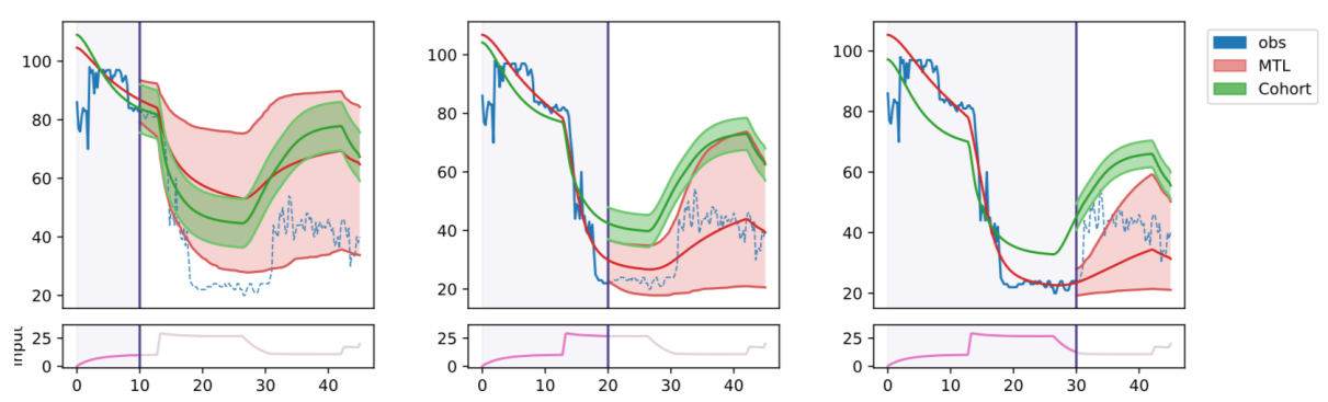
Figure 2: Example predictions for BIS channel at T=10, 20, 30 minutes (left-to-right) for cohort and MTL ($k=5$) models. Shown are the predictive mean and 90% (approx.) credible interval of the underlying function. Retrospective fits are shown without intervals for clarity. Best viewed in colour.

4 RELATED WORK

There is a substantial literature on multi-task learning (MTL) when there is iid input-output data for each task, see e.g. the review paper by Zhang and Yang (2017). This may involve learning a hidden-unit representation shared across tasks (see e.g. Caruana, 1993), low rank structure over the task parameters (see e.g. Ando and Zhang, 2005) or task clustering (see e.g. Bakker and Heskes, 2003). If a vector of “task descriptors” is available for each task, these can be used in MTL, see e.g. Bonilla et al. (2007).

There is some literature on MTL for time series models. For example Dürichen et al. (2015) consider multi-task Gaussian processes (GPs) for condition monitoring of patients, but in their case the multi-task nature is over multiple obervation channels, not patients, and they make use of GP methods for modelling the correlation between channels (see also Bonilla et al. 2008).

Like us Schulam and Saria (2015) do consider multiple patients, but assume an additive decomposition of population, subpopulation, individual and noise components, so ‘individual level’ contributions work as offsets to the population and subpopulation effects. In contrast our eq. (6) uses a more general low-rank structure. Alaa et al. (2018) use patient-specific covariates to personalise a mixture of GPs, but control inputs are not considered, and personalisation is restricted to a fixed set of subtypes. In Automatic Speech Recognition a similar concept called ‘i-vectors’ (Kenny, 2005) is used for speaker personalisation, but does not adapt dynamics or handle control inputs.

A key assumption made by multi-task GP approaches is that tasks are a linear combination of the same set of underlying processes, which is usually inappropriate if the experimental units are separated in time and/or space. We avoid this difficulty by performing multi-task learning of the parameters rather than the processes. Our MTL framework is therefore not merely performing customisation across similar tasks (as in the independent data case), nor gaining strength over latent processes (as for MT GP models), but performing model customisation at the level of experimental units.

Our methodology is in some sense similar to random effects used in the frequentist statistical context, which has seen some development for time series. However, the purpose of such work has largely been to gain strength over individual parameters within a cohort. We are instead looking to exploit relationships between parameters to facilitate faster adaptation and improved prediction in an MTL sense. Furthermore, random effects are usually applied in specific ways, such as only to the emissions (Tsimikas and Ledolter, 1997) or only to the dynamics (Zhou et al., 2013), and with non-general learning algorithms.

5 EXPERIMENTS

In this section we discuss our experimental set-up and results. Section 5.1 introduces the clinical data source, models and training objective, Section 5.2 summarises the results and Section 5.3 concludes with a discussion.

Table 1: 20 and 40-step RMSE and 40-step negative log likelihood (NLL) for all channels, calculated out-of-sample. For all metrics, smaller is better.

		$t=12$ m			$t=24$ m
		RMSE	RMSE	NLL	RMSE	RMSE	NLL
		20-ahead	40-ahead	20-ahead	20-ahead	40-ahead	20-ahead
	Cohort	6.62	7.78	133.84	7.44	7.51	131.08
	MTL-5	6.38	7.71	138.59	5.43	6.15	124.88
BPsys	MTL-7	6.43	7.77	136.91	5.42	6.00	124.05
	STL	11.34	13.65	159.61	7.03	8.48	140.22
	Task-ID	6.82	8.16	137.23	8.39	8.87	138.31
	Cohort	3.74	4.27	110.76	4.31	4.32	109.36
	MTL-5	4.08	4.69	118.23	3.58	3.88	109.07
BPdia	MTL-7	4.19	4.74	119.57	3.63	3.73	109.45
	STL	5.46	6.61	132.20	5.58	5.91	126.33
	Task-ID	4.21	4.92	117.59	4.36	4.64	114.07
	Cohort	10.76	12.28	153.11	11.26	11.60	151.10
	MTL-5	10.01	13.29	155.01	9.31	10.13	140.74
BIS	MTL-7	9.77	13.63	156.48	9.14	9.98	140.84
	STL	14.61	23.25	184.13	10.06	12.62	150.43
	Task-ID	12.35	14.79	160.21	12.71	13.27	155.66

5.1 Experimental set-up

Data

Our data were obtained from an anaesthesia study carried out at the Golden Jubilee National Hospital in Glasgow, Scotland, as described in Georgatzis et al. (2016). These are time series of $N=40$ patients of median length 36 minutes (range approx. 27 - 50 mins) in length and subsampled to 15 second intervals. There are usually $d=3$ channels: BPsys, BPdia and BIS channels, but 11 patients are missing BIS. Obvious artefactual processes (such as instrument dropout or clear exogenous stimulation) were annotated and removed; all such data were marked as missing in the output data. The input data series were volumes administered by the TCI pump, which were converted into inputs $\{u_{t}^{i}\}$ by application of the PK model of White et al. (2008) using ode45 in MATLAB. Each patient had additional covariates of age, gender, height, weight (and BMI).

Models and objective

MTL models are implemented as described in Section 3 and listed as MTL-$k$. The $k$ refers to the subspace dimension, excluding patient offsets, since all models infer these parameters. We also implement a task-description model ‘Task-D’ where the $\mathbf{z}^{i}$ are taken as the covariates of patients as listed above. Models are trained via maximum likelihood, and predictive accuracy is reported via Root Mean Squared Error (RMSE) and log likelihood. The variance $\tau^{-1}$ calculated during training is not optimised for prediction; we report an upper bound on likelihood by optimising $\tau$ in each predictive window, patient, channel and model. All metrics are calculated out-of-sample, for which we use a leave-one-out (LOO) prediction scheme.

In practice the iid modelling assumptions are violated significantly. This was not especially problematic during training, but caused substantial problems for inference on shorter sequences at test time. On a number of occasions, un-modelled noise processes in the data resulted in implausible predictions with high confidence. A simple approach that appears to alleviate this problem is to downsample the observation data given to the inference algorithm by a factor of 4. This removes all significant partial autocorrelations seen in the residuals; predictions are still made on the full data. A further model violation was discovered at the initial stages of the time series. Many patients had elevated vital signs (some had systolic BP above 200), which may be explained by anxiousness prior to a surgical procedure. Since we have no record of steady state vital signs, but the MTL fit showed strong evidence of downwards bias in the first four minutes, we discarded these initial datapoints during inference at test time.

Benchmark models

A one-size-fits-all cohort model is optimised over all patients, with only the patient-specific offsets $\{\bm{\alpha}^{i}\}$ inferred for the predictive posterior. This is an improvement to the state-of-the-art in PK/PD modelling, which does not adapt online. A single-task model was implemented for comparison using relatively uninformative zero-mean Gaussian priors on each parameter with standard deviation $100$. These represent the two extremes of which MTL sits in the middle.

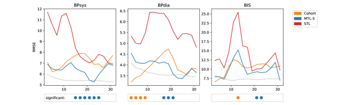
(a) 20-step ahead Predictive RMSE

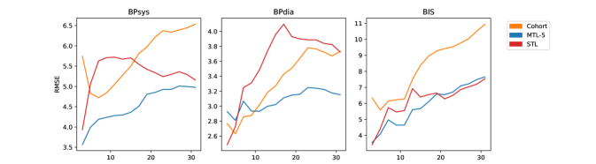
(b) Retrospective RMSE (all preceding datapoints)

Figure 3: Performance over time (in mins). In 3(a), the lower dotted line indicates the avg. error for the retrospective fit of the optimal PD function over each task. If the MTL or Cohort model is significantly better than the other (see text), it is shown as the relevant coloured dot below. Best viewed in colour.

5.2 Results

Figure 2 illustrates the behaviour of the MTL and cohort models on the BIS channel of one patient. The central compartment concentration $u_{t}$ is shown at the bottom of the plot. Credible intervals show the predictive posterior for the underlying PD function after three different time points. The Cohort model (green) is fixed in shape and updates its offset as more datapoints are seen; the MTL model permits much greater flexibility as seen by its adaptation and credible intervals. The MTL model is using data from all 3 channels, but BPsys and BPdia are not shown. Only MTL-5 is shown for clarity; the performance of MTL-7 is very similar in almost all tasks. More examples are shown in supp. mat.

Figure 3(a) shows the 20-step-ahead (or 5-mins-ahead) RMSE for the Cohort, MTL and STL models for the BPsys, BPdia and BIS channels, averaged over LOO patients. Table 1 gives these results for each channel for times $t=12$ mins and $t=24$ mins, along with 40-step-ahead RMSE and negative log likelihood (for all columns lower is better). There is a clear win for MTL over STL in the plots for the first 30 minutes of infusion. The benefit is sustained across all time points in this initial period, but observe the STL model is ‘closing the gap’ as we approach the 30 minute mark. Notice that prediction errors show some dependence on time, particularly after large changes due to infusion scheduling (see appendix A.1) at approximately 13 mins. and again after 27 mins.

Comparing MTL and the Cohort model, the results are closer, but MTL broadly out-performs the Cohort model on aggregate after 15 minutes of observations, although the performance drops back at the infusion change at approx. 27 minutes. It is not so surprising that the Cohort model does better early on, as it has fewer latent variables to estimate than the MTL model. Many of these improvements are significant according to a $p<0.05$ Wilcoxon signed-rank test as shown under Figure 3(a), although no adjustment has been made for multiple testing (such as a Bonferroni correction). Table 1 demonstrates that these features are also retained in a longer predictive interval.

The performance of the patient covariate model Task-D is also given in Table 1. It performs worse in general than the Cohort model and does not perform substantially better even on the training set. This is indicative of a lack of information in our patient covariates. Use of more complex models such as Long Short Term Memory (LSTM, Hochreiter and Schmidhuber, 1997) networks in preliminary investigations also supported this conclusion. In principle one could combine the unsupervised MTL method with the task descriptors, but no benefit would be expected on this dataset.

Fig. 3(b) shows the retrospective RMSE as a function of time for the different models, based on “post-dicting” the the data seen up to time $t$ given the inferences for $\mathbf{z}$ at time $t$. These plots show that the MTL model is substantially better at this task than the Cohort and STL models for both BP channels.

5.3 Discussion

The results in Section 5.2 demonstrate that the MTL framework can achieve a predictive RMSE close to that obtained by the optimal function in the PD class, as shown by the dotted line in Figure 3(a). This represents the predictive RMSE of the best-fitting PD function of form (5) fitted retrospectively per patient on the test set.

Two major factors in the data elevate the minimum achievable RMSE for the PD model. Firstly, even with obvious artefacts removed, there remain many other exogenous ‘events’ which cannot be explained by the model. Secondly, the relative level of peaks and troughs for a given patient (particularly in BIS) cannot always be adequately fitted with the PD model. The changes sometimes appear more like input-driven phase changes (see e.g. Mukamel et al. 2014). Thus a more flexible (deterministic) model class may not improve the fit very much.

The performance of the Cohort PD model is surprisingly good. Traditionally, PD models have adaptive offsets based on covariates, and practicing anaesthetists may mentally perform further customisation. Our work is the first instance (to our knowledge) of investigating an online estimation of these offsets over several channels, and our Cohort PD model appears to outperform those generally used in practice. Nevertheless, the Cohort model does not fit well retrospectively (Fig. 3(b)) which indicates both that it does not capture the inter-patient variation, and that it may perform poorly in future – that is, if the past is representative of the future.

The worsening performance of the MTL model as $t$ approaches 30 minutes is due to a changepoint in the infusion schedule (see appendix A.1). These changepoints occur twice in the infusion sequences at approx. $t=13$ and $t=27$ minutes and clearly present a more challenging part of the task. The data observed so far may contain little information about the response here, and perhaps in future the infusion sequence can be designed to be more informative.

An important result given by the Task-D model is the failure of patient covariates to improve performance. While there appears to be very little information about vitals shape available in the covariates, some information about level may be expected had we not estimated offsets online. Note that the covariates have already been used to personalise the upstream PK model.

6 CONCLUSION

In this paper we have presented a method for extending the multi-task learning framework to collections of sequential tasks. We have seen via use of the drug-response example that MTL can improve the aggregate performance of a collection of discrete time input-output dynamical systems over either a cohort or single-task approach. Time series without control inputs can be handled equally well. The framework is of course more general than the use case in this paper and we are actively exploring other areas of application.

The application of this framework to the PK/PD modelling problem provides a novel approach to personalised medicine, and at least in this case shows substantial promise over traditional methods which personalise using patient covariates. Where patient covariates contain such a low signal, an unsupervised approach is essential for better performance, and a larger dataset per se will not help much. Further improvements in this approach may be possible by incorporating artefact models and the optimal design of infusion sequences.

There are other important findings that may be of interest to a clinical audience. For example, in defining a benchmark PD model, we have proposed a PD model that is better than usually used in clinical practice, which we have improved further using MTL. In some tasks, correlations learned between channels via latent variables have led to useful predictions even for a channel that has dropped out. Finally, the loading matrix $\Psi$ may be of direct interest in itself; we leave a disentangled representation to future work.

Appendix A APPENDIX

A.1 Infusion Schedule

The volumes of Propofol infused during each experiment followed one of two regimes: a high-low-high dose or a low-high-low dose. 18 patients were allocated to the first group, 22 patients to the second. Despite differences in regimes and volumes, the changepoints between types of dosage happened at approximately the same time. After 27-30 minutes, the MTL models are observing a low-high or high-low transition for the first time. Prior to observing this information, it is difficult to out-perform an average effect.

Figure 4 plots each of the different inputs $\{u_{t}^{i}\}$ over all patients, split into these regimes. Note that these are the central compartment solutions to the PK equation (1) using personalised rate constants and exhibit substantial variation in magnitude.

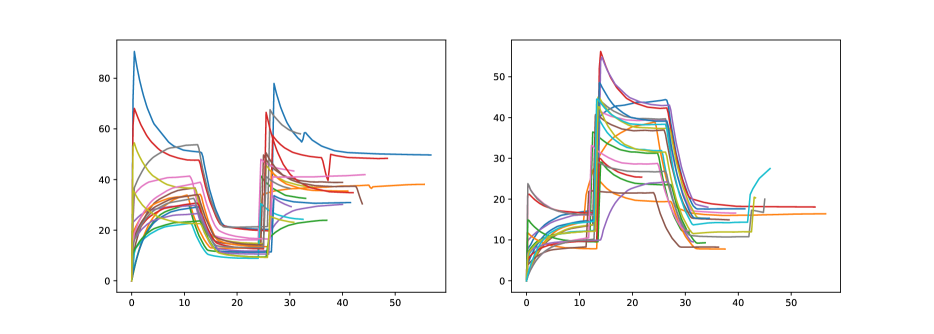
Figure 4: Inputs $\{u_{t}^{i}\}$ for all patients. Different regimes are split into separate panels for clarity.

References

- Alaa et al. (2018) A. M. Alaa, J. Yoon, S. Hu, and M. van der Schaar. Personalized Risk Scoring for Critical Care Prognosis using Mixtures of Gaussian Processes. IEEE Transactions on Biomedical Engineering, 65(1):207–218, 2018.
- Ando and Zhang (2005) R. K. Ando and T. Zhang. A Framework for Learning Predictive Structures from Multiple Tasks and Unlabeled Data. Journal of Machine Learning Research, 6(Nov):1817–1853, 2005.
- Bailey and Haddad (2005) J. M. Bailey and W. M. Haddad. Drug Dosing Control in Clinical Pharmacology. IEEE Control Systems, 25(2):35–51, 2005.
- Bakker and Heskes (2003) B. Bakker and T. Heskes. Task Clustering and Gating for Bayesian Multitask Learning. Journal of Machine Learning Research, 4(May):83–99, 2003.
- Bonilla et al. (2008) E. Bonilla, K. M. A. Chai, and C. K. I. Williams. Multi-task Gaussian Process Prediction. In J. Platt, D. Koller, Y. Singer, and S. Roweis, editors, Advances in Neural Information Processing Systems 20, pages 153–160. MIT Press, Cambridge, MA, 2008.
- Bonilla et al. (2007) E. V. Bonilla, F. V. Agakov, and C. K. Williams. Kernel Multi-Task Learning Using Task-Specific Features. In International Conference on Artificial Intelligence and Statistics, pages 43–50, 2007.
- Carpenter et al. (2016) B. Carpenter, A. Gelman, M. Hoffman, D. Lee, B. Goodrich, M. Betancourt, M. A. Brubaker, J. Guo, P. Li, A. Riddell, et al. Stan: A Probabilistic Programming Language. Journal of Statistical Software, 20(2):1–37, 2016.
- Caruana (1993) R. Caruana. Multitask Learning: A Knowledge-Based Source of Inductive Bias. In Proceedings of the Tenth International Conference on Machine Learning, pages 41–48, 1993.
- Chopin (2002) N. Chopin. A Sequential Particle Filter Method for Static Models. Biometrika, 89(3):539–552, 2002.
- Del Moral et al. (2006) P. Del Moral, A. Doucet, and A. Jasra. Sequential Monte Carlo Samplers. Journal of the Royal Statistical Society: Series B (Statistical Methodology), 68(3):411–436, 2006.
- Dürichen et al. (2015) R. Dürichen, M. A. Pimentel, L. Clifton, A. Schweikard, and D. A. Clifton. Multitask Gaussian Processes for Multivariate Physiological Time-Series Analysis. IEEE Transactions on Biomedical Engineering, 62(1):314–322, 2015.
- Eleveld et al. (2018) D. Eleveld, P. Colin, A. Absalom, and M. Struys. Pharmacokinetic–Pharmacodynamic Model for Propofol for Broad Application in Anaesthesia and Sedation. British Journal of Anaesthesia, 120(5):942–959, 2018.
- Georgatzis et al. (2016) K. Georgatzis, C. K. I. Williams, and C. Hawthorne. Input-Output Non-Linear Dynamical Systems applied to Physiological Condition Monitoring. Machine Learning for Healthcare, 2016.
- Glen and Servin (2009) J. Glen and F. Servin. Evaluation of the Predictive Performance of Four Pharmacokinetic Models for Propofol. British Journal of Anaesthesia, 102(5):626–632, 2009.
- Glen and White (2014) J. Glen and M. White. A Comparison of the Predictive Performance of Three Pharmacokinetic Models for Propofol Using Measured Values Obtained During Target-Controlled Infusion. Anaesthesia, 69(6):550–557, 2014.
- Hill (1910) A. V. Hill. The Possible Effects of the Aggregation of the Molecules of Haemoglobin on its Dissociation Curves. The Journal of Physiology, 40:4–7, 1910.
- Hochreiter and Schmidhuber (1997) S. Hochreiter and J. Schmidhuber. Long Short-Term Memory. Neural Computation, 9(8):1735–1780, 1997.
- Hoffman and Gelman (2014) M. D. Hoffman and A. Gelman. The No-U-Turn Sampler: Adaptively Setting Path Lengths in Hamiltonian Monte Carlo. Journal of Machine Learning Research, 15(1):1593–1623, 2014.
- Jelliffe (1967) R. W. Jelliffe. A Mathematical Analysis of Digitalis Kinetics in Patients with Normal and Reduced Renal Function. Mathematical Biosciences, 1(2):305–325, 1967.
- Kenny (2005) P. Kenny. Joint Factor Analysis of Speaker and Session Variability: Theory and Algorithms. CRIM, Montreal,(Report) CRIM-06/08-13, 14:28–29, 2005.
- Kingma and Ba (2014) D. P. Kingma and J. Ba. Adam: A Method for Stochastic Optimization. In Proceedings of the 3rd International Conference on Learning Representations, 2014.
- Marsh et al. (1991) B. Marsh, M. White, N. Morton, and G. Kenny. Pharmacokinetic Model Driven Infusion of Propofol in Children. British Journal of Anaesthesia, 67(1):41–48, 1991.
- Masui et al. (2010) K. Masui, R. N. Upton, A. G. Doufas, J. F. Coetzee, T. Kazama, E. P. Mortier, and M. M. Struys. The Performance of Compartmental and Physiologically Based Recirculatory Pharmacokinetic Models for Propofol: a Comparison Using Bolus, Continuous, and Target-Controlled Infusion Data. Anesthesia & Analgesia, 111(2):368–379, 2010.
- McLachlan and Krishnan (2007) G. McLachlan and T. Krishnan. The EM Algorithm and Extensions, volume 382. John Wiley & Sons, 2007.
- Minto and Schnider (2008) C. Minto and T. Schnider. Contributions of PK/PD Modeling to Intravenous Anesthesia. Clinical Pharmacology & Therapeutics, 84(1):27–38, 2008.
- Mukamel et al. (2014) E. A. Mukamel, E. Pirondini, B. Babadi, K. F. K. Wong, E. T. Pierce, P. G. Harrell, J. L. Walsh, A. F. Salazar-Gomez, S. S. Cash, E. N. Eskandar, et al. A Transition in Brain State During Propofol-Induced Unconsciousness. Journal of Neuroscience, 34(3):839–845, 2014.
- Myles et al. (2004) P. Myles, K. Leslie, J. McNeil, A. Forbes, M. Chan, B.-A. T. Group, et al. Bispectral Index Monitoring to Prevent Awareness During Anaesthesia: the B-Aware Randomised Controlled Trial. The Lancet, 363(9423):1757–1763, 2004.
- Neal et al. (2011) R. M. Neal et al. MCMC Using Hamiltonian Dynamics. Handbook of Markov Chain Monte Carlo, 2(11), 2011.
- Paszke et al. (2017) A. Paszke, S. Gross, S. Chintala, G. Chanan, E. Yang, Z. DeVito, Z. Lin, A. Desmaison, L. Antiga, and A. Lerer. Automatic Differentiation in PyTorch. 2017.
- Schnider et al. (1998) T. W. Schnider, C. F. Minto, P. L. Gambus, C. Andresen, D. B. Goodale, S. L. Shafer, and E. J. Youngs. The Influence of Method of Administration and Covariates on the Pharmacokinetics of Propofol in Adult Volunteers. The Journal of the American Society of Anesthesiologists, 88(5):1170–1182, 1998.
- Schulam and Saria (2015) P. Schulam and S. Saria. A Framework for Individualizing Predictions of Disease Trajectories by Exploiting Multi-Resolution Structure. In Advances in Neural Information Processing Systems 28, pages 748–756, 2015.
- Tsimikas and Ledolter (1997) J. V. Tsimikas and J. Ledolter. Mixed Model Representation of State Space Models: New Smoothing Results and their Application to REML Estimation. Statistica Sinica, pages 973–991, 1997.
- White et al. (2008) M. White, G. N. Kenny, and S. Schraag. Use of Target Controlled Infusion to Derive Age and Gender Covariates for Propofol Clearance. Clinical Pharmacokinetics, 47(2):119–127, 2008.
- Xue et al. (2007) Y. Xue, X. Liao, L. Carin, and B. Krishnapuram. Multi-Task Learning for Classification with Dirichlet Process Priors. Journal of Machine Learning Research, 8(Jan):35–63, 2007.
- Zhang and Yang (2017) Y. Zhang and Q. Yang. A Survey on Multi-Task Learning. arXiv preprint arXiv:1707.08114, 2017.
- Zhou et al. (2013) J. Zhou, L. Han, and S. Liu. Nonlinear Mixed-Effects State Space Models with Applications to HIV Dynamics. Statistics & Probability Letters, 83(5):1448–1456, 2013.