Volumetric Untrimming:
Precise decomposition of trimmed trivariates into tensor products

Abstract

3D objects, modeled using Computer Aided Geometric Design (CAGD) tools, are traditionally represented using a boundary representation (B-rep), and typically use spline functions to parameterize these boundary surfaces. However, recent development in physical analysis, in isogeometric analysis (IGA) in specific, necessitates a volumetric parametrization of the interior of the object. IGA is performed directly by integrating over the spline spaces of the volumetric spline representation of the object. Typically, tensor-product B-spline trivariates are used to parameterize the volumetric domain.

A general 3D object, that can be modeled in contemporary B-rep CAD tools, is typically represented using trimmed B-spline surfaces. In order to capture the generality of the contemporary B-rep modeling space, while supporting IGA needs, Massarwi and Elber [2016] proposed the use of trimmed trivariates volumetric elements. However, the use of trimmed geometry makes the integration process more difficult since integration over trimmed B-spline basis functions is a highly challenging task Xu et al. [2017]. In this work, we propose an algorithm that precisely decomposes a trimmed B-spline trivariate into a set of (singular only on the boundary) tensor-product B-spline trivariates, that can be utilized to simplify the integration process, in IGA. The trimmed B-spline trivariate is first subdivided into a set of trimmed Bézier trivariates, at all its internal knots. Then, each trimmed Bézier trivariate, is decomposed into a set of mutually exclusive tensor-product B-spline trivariates, that precisely cover the entire trimmed domain. This process, denoted untrimming, can be performed in either the Euclidean space or the parametric space of the trivariate. We present examples of the algorithm on complex trimmed trivariates’ based geometry, and we demonstrate the effectiveness of the method by applying IGA over the (untrimmed) results.

1 Introduction

Tensor product (Bézier, B-spline and NURBS) surfaces are widely used in CAGD due to their simple structure, mathematical form, and powerful geometrical properties, that make them intuitive to use. Consider the parametric representation of a tensor product B-spline volume:

Definition 1.

A B-spline parametric trivariate is a volumetric extension to parametric B-spline curves and surfaces, with a three dimensional parametric space Cohen et al. [2002]. A common representation of trivariates is by tensor product B-splines, as:

$$T(u,v,w)=\sum_{i=0}^{l}\sum_{j=0}^{m}\sum_{k=0}^{n}P_{i,j,k}B_{i,d_{u}}(u)B_{j,d_{v}}(v)B_{k,d_{w}}(w),$$ (1)

where $T$ is defined over the 3D parametric domain $[U_{min},U_{max})\times[V_{min},V_{max})\times[W_{min},W_{max})$, $P_{i,j,k}\in\rm I\!R^{q}$, $q\geq 3$ are the control points of $T$, and $B_{i,d}$ is the $i$’th univariate B-spline basis functions of degree $d$.

3D geometric objects, generated with contemporary computer aided geometric design (CAGD) systems, are almost solely exploiting a boundary representation (B-rep), where these objects’ boundaries are represented as trimmed parametric surfaces. In recent years, with recent developments of additive manufacturing and 3D printing as well as analysis, the demand for a full volumetric representation (V-rep) is increasing. Volumetric modeling of the inside of the object, as oppose to only its boundary (B-rep), can be used to describe different volumetric properties such as materials or stresses, in scalar, vector or tensor fields. Developments in physical analysis, isogeometric analysis (IGA) in specific Cottrell et al. [2009], employs a parametrization of the object’s volume. In IGA, the analysis is performed by integrating in the same spline spaces that describe the geometry.

Tensor product trivariates are limited to a cuboid topology, making them difficult to use in creating general 3D objects, having an arbitrary topology. That is, the cuboid topology does not allow one to represent with ease general shapes, including holes. Similar to trimmed surfaces, that enriches the B-rep modeling space of the set of objects that can be represented using tensor product surfaces Cohen et al. [2002], trimmed trivariates can be used to create far more general volumetric objects, compared to tensor products. A framework for a volumetric representation (V-rep) modeling is proposed in Massarwi and Elber [2016], that suggests a representation for a general volumetric model (V-model) as well as V-model constructors and Boolean operations algorithms on V-models. In Massarwi and Elber [2016], a V-model is composed of volumetric elements called V-cells, where each V-cell relates to one or more (intersecting) trivariate(s), and is defined as following:

Definition 2.

A V-rep cell (V-cell) is a 3-manifold that is defined over of one or more (intersecting) B-spline tensor product trivariates. The sub-domain of the V-cell is delineated by trimming surfaces.

In this work, we follow the definition of a V-cell in Massarwi and Elber [2016], selecting one tensor product trivariate from the V-cell to be associate with the V-cell and parameterize it. Then, we define a trimmed trivariate as following:

Definition 3.

Trimmed trivariate ${\cal T}$ is defined in the domain of a containing tensor product trivariate $T$ and has a set of (possibly trimmed) surfaces ${\cal S}$ as the trimming surfaces of $T$, forming a 2-manifold in the domain of $T$.

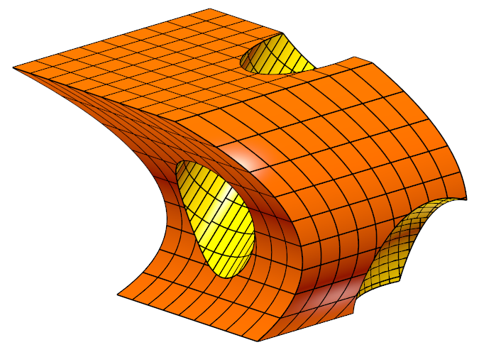
The trimming surfaces in ${\cal S}$ can be classified into two groups. The first type of the trimming (trimmed) surfaces are (trimmed) boundary surfaces of $T$. The second type are trimming (trimmed) surfaces that are (trimmed) boundary surfaces of some other trivariates, ${\cal F}_{i}$, that are results of volumetric Boolean operations Massarwi and Elber [2016] between ${\cal T}$ and ${\cal F}_{i}$. Note that, in Massarwi and Elber [2016], trimming (trimmed) surfaces of the second type are not defined explicitly in the parametric space of $T$, but only in the Euclidean space. Figure 1(a) shows an example of a trimmed trivariate.

In IGA, the analysis is performed directly in a spline space employing (suitable) integration over the (trimmed) volumetric domain of the object, which herein means integration over trimmed trivariates. However, integration over trimmed B-spline basis functions is a highly challenging task Xu et al. [2017]. Methods to precisely integrate over the trimming domains are required, in order to support a complete and accurate IGA over trimmed-trivariates. One way to achieve this goal, is by decomposing the trimmed-trivariates to tensor-products.

In this work, we present a volumetric untrimming process for trimmed trivariate:

Definition 4.

The Untrimming of a trimmed trivariate ${\cal T}$, is a process in which ${\cal T}$ is decomposed into a set of (potentially singular on the boundaries) mutually exclusive tensor-product B-spline trivariates that precisely cover the entire trimmed volume of ${\cal T}$.

A trivariate $T$ is considered potentially singular on the boundary if the Jacobian of $T$ can vanish only at the boundaries, and $T$ is self intersection free.

The resulting set of tensor product trivariates can be utilized to simplify the integration process in IGA, as the integration will be performed over a non-trimmed B-spline basis functions with full support. In the untrimming algorithm to be presented in this work, the trimmed-trivariate is first subdivided into trimmed Bézier trivariates, at all its internal knots. Then, each trimmed Bézier trivariate is decomposed into a set of tensor-product B-spline trivariates. The untrimming algorithm can be performed either in the Euclidean space or the parametric space of the trimmed trivariate.

It is important to remark that, on the contrary to classical finite element and IGA methods, in which the solution quality is intrinsically linked to the mesh quality, that is not the case in the present approach. In the analysis, the tensor-product trivariates created during the untrimming process are exclusively used for computing the integrals involved in Galerkin problems. Therefore, the solution discretization is not related to the untrimming result and its quality is not conditioned by the untrimming trivariates’ Jacobians. We refer the interested reader to Marussig and Hughes [2018], and references therein, where the numerical computation of integrals in trimmed domains using untrimming tiles is discussed.

The rest of this document is organized as follows. Section 2 discusses related work. In Section 3, the volumetric untrimming algorithm is introduced. In Section 4, some results of the untrimming algorithm are introduced, and in Section 5, an IGA application over trimmed trivariates, utilizing the presented untrimming algorithm, is presented. Finally, Section 6 concludes this effort and discusses possible future work.

Figure 1: Subdivision of a trimmed B-spline trivariate into trimmed Bézier trivariates, shown in Euclidean space. (a) A trimmed B-spline trivariate, having two internal knots at each parametric direction. Trimmed trimming surfaces on the boundaries of the trivariate have an orange color, and non-boundary trimmed trimming surfaces are colored with yellow. (b) The iso parametric surfaces of the internal knots (in green). (c) Twenty eight (and not twenty seven!) trimmed Bézier trivariates in an exploded view, as result of all the subdivisions along the iso parametric knot surfaces (in (b)).

2 Previous work

Many algorithms have been proposed for hexahedral meshing of 2-manifold polygonal meshes, i.e Armstrong et al. [2015], Yu et al. [2015]. Given a trimmed trivariate, hexahedral meshing algorithms can be applied to a polygonal mesh which is an approximation mesh of the boundary surfaces of the trimmed trivariate, only to generate hexahedral elements that cover the trimmed domain. Then, a trilinear tensor product trivariate can be extracted from each hexahedron. However, there are two conceptual drawbacks of such approach. First, the boundaries of the trimmed trivariate are approximated, which introduces an error which might lead to instabilities in the integration and analysis processes. Second, all the generated tensor product trivariates are of linear order, where in IGA, basis functions of a higher order (and continuity) are typically handled (and desired). An extensive review of the existing isogeometric techniques for trimmed domains, mostly in the context of trimmed surfaces, is presented in Marussig and Hughes [2018].

Meshing tools and algorithms are a long and large subject of research in the finite element community. For example, Geuzaine and Remacle [2009] introduce Gmsh, a commonly used tool for mesh generation that is suitable for finite element analysis, including of B-spline surfaces. Starting from a B-rep model, the boundary (trimmed) surfaces are triangulated, and then methods for tetrahedral mesh generation are applied to generate finite elements approximating the enclosed volume of the B-rep model. In addition to the drawbacks discussed above when applying tetrahedral mesh generation algorithms, the generated elements in Gmsh only approximate the boundary surfaces, and an optimization process needs to be applied in order to reduce the approximation error. Specifically, the tool is not sufficient for IGA needs, as in IGA, the integration should be performed in the parametric domain of the underlying trivariate, where the integration boundaries shouldn’t cross knot values. Hence, method for subdividing the trimmed B-spline trivariate into trimmed Bézier trivariates as well as further processing of trimmed Bézier trivariates are required, and such tools are not available in Gmsh.

Other studies, such as Martin and Cohen [2010], suggests volumetric spline parametrization of a (B-rep) polygonal mesh. Although generating high order trivariates, and since the input is a discrete triangulated mesh, it is not clear how to utilize such an approach in a design process, while Martin and Cohen [2010] can serve as another way of synthesizing trivariates.

In Xu et al. [2013], a volumetric parametrization of a multi-block computational domain is provided, where the computation domain is segmented into several blocks, and each block is bounded by six tensor product 2D faces that are used to generate a trivariate. An iterative process of moving the trivariate’s control points is then applied in order to achieve a better analysis suitable parametrization. The optimization process improves uniformity of the Jacobian for each trivariate as well as smoothness between trivariates. However, the method in Xu et al. [2013] assumes full computational domains, and doesn’t handle trimmed trivariates.

Zhu et al. [2016] propose B++ splines; trimmed B-spline basis functions that are developed to perform IGA on trimmed B-rep models. In order to handle arbitrary trimming curves, the trimmed spline basis functions are defined over samples of trimming curves. Such sampling introduces inaccuracies, and trimmed surfaces with sharp and complex boundaries require dense sampling in order to achieve a certain accuracy. The inaccuracy is delegated to the analysis stage as the method in Zhu et al. [2016] requires conversion of the B-rep trimmed spline surfaces into B++ surfaces.

In Liu et al. [2014], T-spline trivariates are extracted from boundary triangulated surfaces, using hierarchical octrees, and Boolean operation of volumetric cylinders and cubes. However, even simple models composed of cones and tetrahedrons cannot be handled by Liu et al. [2014].

An analysis suitable trivariate parametrization for a B-rep model is suggested in Engvall and Evans [2017]. First, the B-rep model is approximated as a polygonal mesh, then the interior of the polygonal mesh is covered with unstructured tetrahedrons, and finally each tetrahedron is replaced with a rational Bézier trivariate with, possibly, faces extracted from the original trimmed surfaces. Unfortunately, the method loses the connection to the input B-rep surfaces, and is largely ignoring the problem of trimming, and assumes non-trimmed surfaces of the B-rep model and thus can not handle trimmed trivariates.

To summarize, previous methods of trivariate volumetric parametrization of general models lack precision or robustness, and cannot handle trimmed B-spline volumes. Additionally, previous methods suggest a solution for B-rep models, and none of them suggest a solution for a general trimmed trivariate, that can result from volumetric Boolean operations.

3 The Untrimming Algorithm

In this section, we present the volumetric untrimming algorithm. Recall Figure 1(a) and consider a trimmed B-spline trivariate ${\cal T}$, following Definition 3, as a tensor product B-spline trivariate $T$, and a set of trimming (trimmed) surfaces, ${\cal S}$. We assume the following on ${\cal T}$, as in Massarwi and Elber [2016]:

• ${\cal S}$ consists of (trimmed) surfaces that together form a 2-manifold B-rep model in the domain of $T$. Note that each surface $S\in{\cal S}$ is a trimming surface of $T$, but $S$ can also be a trimmed surface on its own.

• Each trimmed surface ${S\in\cal S}$ is orientable and the normal at each point on $S$ points toward the inside of ${\cal T}$.

The untrimming algorithm decomposes ${\cal T}$ into a set of mutually exclusive tensor product trivariates that covers the volume enclosed by ${\cal T}$ and precisely interpolates the boundary (trimming surfaces). The untrimming can be performed either in the Euclidean space, where the algorithm is applied directly over the 3D geometry of ${\cal T}$, or in the parametric space of $T$, where the algorithm is applied on the trimmed parametric domain of $T$. The result of the untrimming in the parametric space, is a set of mutually exclusive tensor product trivariates $\tau$, such that $T(\tau)$ completely covers ${\cal T}$, in the Euclidean space.

Some simple applications, such as enclosed volume computation, can be performed by summing the enclosed volume of each of the tensor product trivariates of the untrimming result in the Euclidean space. However, in general integration applications, the untrimming needs to be performed in the trimmed parametric domain. In the next sub-sections, we describe the untrimming algorithm in the parametric space (i.e the final output is a set of tensor product B-spline trivariates in the parametric space of $T$, that covers the trimmed domain). The untrimming in the Euclidean space can be considered as a special case of the algorithm, having the bounding box of ${\cal T}$ as the associated trivariate $T$.

The algorithm consists of two main stages: In the first stage, discussed in Section 3.1, ${\cal T}$ is subdivided into trimmed Bézier trivariates at all the knot planes of $T$. In the second stage, discussed in Section 3.2, each trimmed Bézier trivariate from the first stage is decomposed into a set of mutually exclusive (possibly singular on the boundary) tensor product B-spline trivariates that cover the domain.

3.1 Subdivision into Bézier trimmed trivariates

The integration of B-spline basis functions is needed in IGA, for example, in the computation of the mass and stiffness matrix elements Bartoň et al. [2017]. In order to use the Gaussian quadrature method Atkinson [2008] for precise computation of the integral over the B-spline basis functions, the B-spline basis functions need to be split into polynomial or rational (in the NURBS case) functions. Bézier elements extraction of a tensor product B-spline functions can be performed by multiple knot insertion Cohen et al. [2002]. However, for the Bézier elements’ extraction from a trimmed B-spline trivariate ${\cal T}$, the trimming (trimmed) surfaces, ${\cal S}$, need to be subdivided as well, along the iso-parametric surfaces of $T$, at all the internal knots of $T$.

Input:
${\cal T}=\{T,{\cal S}\}$: A trimmed B-spline trivariate; $T$ is a tensor product B-spline trivariate, that is trimmed by set of trimmed surfaces ${\cal S}$; $t,dir$: Subdivision parameter, $t$, of $T$, in parametric direction $dir$: $u,v$ or $w$; Output:
${\cal T}_{t}^{dir}$: A set of trimmed trivariates which are the result of subdividing ${\cal T}$ at parameter $t$ in direction $dir$;
// The following auxiliary function constructs a set of trimmed trivariates by trimming the trivariate $T$,
// with a set of trimming (trimmed) surfaces, ${\cal S}$.
Function GroupNewTrimTV(${\cal S},T$)

1:  ${\cal T}_{Res}:=\emptyset$;

2:  if ${\cal S}\neq\emptyset$ then

3:     ${\cal{CS}}$ := Group ${\cal S}$ into sets of 2-manifold connected closed component surfaces;

4:     for all ${\cal S}_{i}\in{\cal{CS}}$ do

5:        ${\cal T}_{i}$ := Trimmed Trivariate {$T$,${\cal S}_{i}$};

6:        ${\cal T}_{Res}:={\cal T}_{Res}\bigcup~{}\{{\cal T}_{i}\}$;

7:     end for

8:  end if

9:  return  ${\cal T}_{Res}$;

Algorithm:

1:  $S_{iso}$ := Iso surface of $T$ at parameter $t$, in direction $dir$;

2:  $\{T_{L},T_{R}\}$ := Subdivided $T$ at parameter $t$, in direction $dir$;

3:  ${\cal S}_{L}$ := Intersect(${\cal S}$,$S_{iso}$); //B-rep Boolean ${\cal S}*S_{iso}$

4:  ${\cal S}_{R}$ := Subtract(${\cal S}$,$S_{iso}$); //B-rep Boolean ${\cal S}-S_{iso}$

5:  ${\cal T}_{t}^{dir}:=\begin{aligned} &\textbf{GroupNewTrimTV}({\cal S}_{L},T_{L})~{}\cup\\ &\textbf{GroupNewTrimTV}({\cal S}_{R},T_{R});\end{aligned}$

6:  return  ${\cal T}_{t}^{dir}$;

Algorithm 1 TrimTrivarSubdiv(${\cal T},t,dir$): Subdivision of a trimmed B-spline trivariate ${\cal T}$ at $t$ along $dir$

Input:
${\cal T}=\{T,{\cal S}\}$: A trimmed B-spline trivariate; $T$ is a tensor product B-spline trivariate, that is trimmed by set of trimmed surfaces ${\cal S}$;

Output:
${\cal B}$: A set of trimmed Bézier trivariates;

Algorithm:

1:  if $T$ is a Bézier trivariate then // COMMENTno internal knots

2:     return  ${\cal T}$;

3:  else

4:     $t,dir$ := Find an internal knot, $t$, of $T$, in parametric direction $dir$ ($u,v$ or $w$);              

5:     ${\cal T}_{t}^{dir}$ := TrimTrivarSubdiv(${\cal T},t,dir$);

6:     ${\cal B}$ := $\emptyset$;

7:     for all ${\cal T}_{i}\in{\cal T}_{t}^{dir}$ do

8:        ${\cal B}$ := ${\cal B}\bigcup$  TrimTVBezierSubd(${\cal T}_{i}$);

9:     end for

10:     return  ${\cal B}$;

11:  end if

Algorithm 2 TrimTVBezierSubd(${\cal T}$): Subdivision of a trimmed trivariate ${\cal T}$ into trimmed Bézier trivariates

Algorithm 1 presents the process of subdividing a given trimmed trivariate, at a given parametric value and direction. Algorithm 2 describes the subdivision algorithm of trimmed trivariate ${\cal T}$, into trimmed Bézier trivariates. Algorithm 2 recursively divides the trimmed trivariate ${\cal T}$, at all the internal knots of $T$, in all parametric directions, using Algorithm 1.

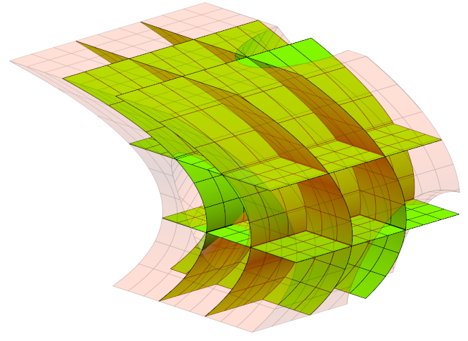
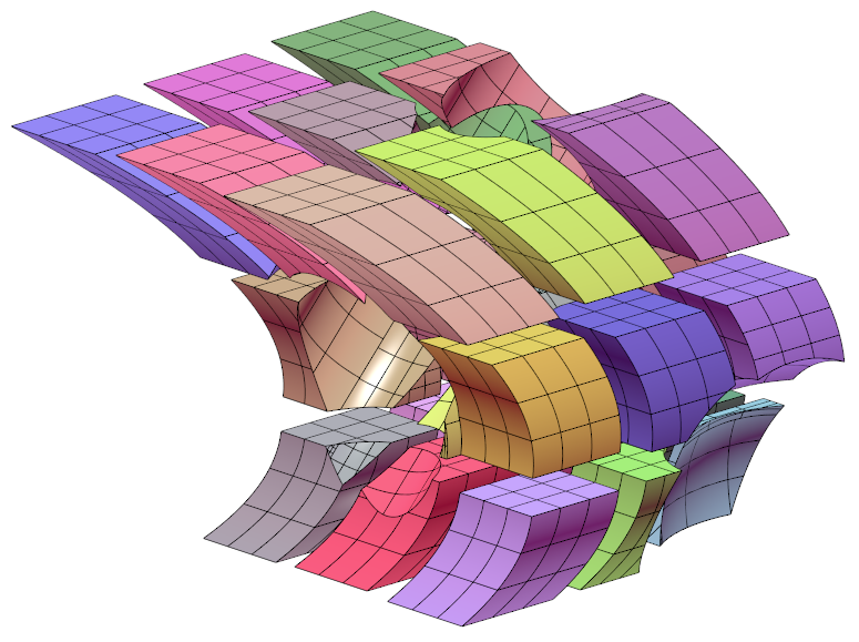
The general trimmed trivariate subdivision algorithm (Algorithm 1) is performed in the Euclidean space, as the trimming surfaces ${\cal S}$ are given, following Massarwi and Elber [2016], in the Euclidean space. In Algorithm 1, $T$ is subdivided at a parametric value $t$, in direction $dir$, resulting in two tensor product trivariates $T_{L}$ and $T_{R}$. The trimming surfaces, ${\cal S}$, are then separated by the iso-surface value $t$, in direction $dir$, $S_{iso}$, into two groups. The separation is done by applying B-rep intersection and subtraction Boolean operations Satoh and Chiyokura [1991], Thomas [1986] between ${\cal S}$ (that forms a closed B-rep), and $S_{iso}$. See lines 3 and 4 in Algorithm 1, where ${\cal S}_{L}$ and ${\cal S}_{R}$ are the result of the intersection and subtraction Boolean operations between ${\cal S}$ and $S_{iso}$ respectively. Such Boolean set operations typically involve computing surface-surface intersections (SSI) that may introduce approximation errors. However, methods for computing SSI have been investigated for a long time (i.e. Grandine and Klein [1997]), including bounds on errors in the SSI. Each iso-parametric surface of $T$, divides $T$ into two parts. However, since the trimming can impose arbitrary topology, each of the two groups (${\cal S}_{L}$ and ${\cal S}_{R}$), from both sides of $S_{iso}$, can consist of multiple connected components of trimming surfaces, see for example Figure 3. For each group of trimming surfaces that forms a connected component, ${\cal S}_{M}$, a trimmed trivariate is constructed in GroupNewTrimTV, having ${\cal S}_{M}$ as the trimming surfaces and either $T_{L}$ or $T_{R}$ (the one that contains ${\cal S}_{M}$) as its tensor product trivariate. See Figures 1-3 for some results of Algorithm 2.

Figure 2: Subdivision of trimmed trivariate (red) in (a) along an iso-parametric surface (yellow) results in five trimmed trivariates: one trimmed trivariate on the back side of the iso-surface in (b), and four trimmed trivariates on the front side of the iso-surface in (c). An exploded view is presented in (b)/(c).

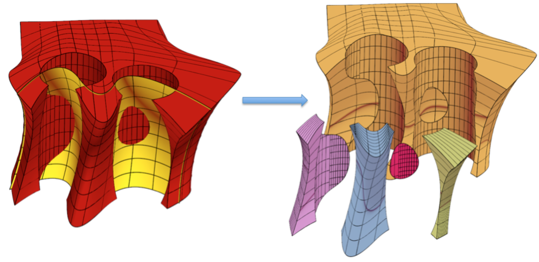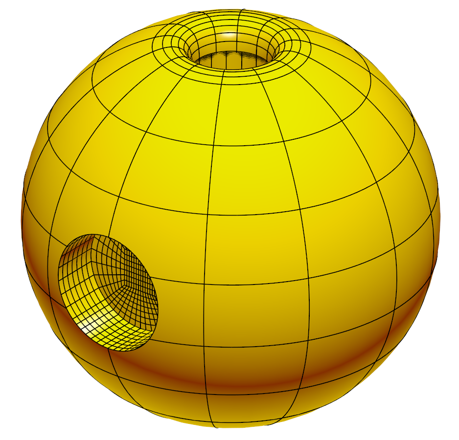
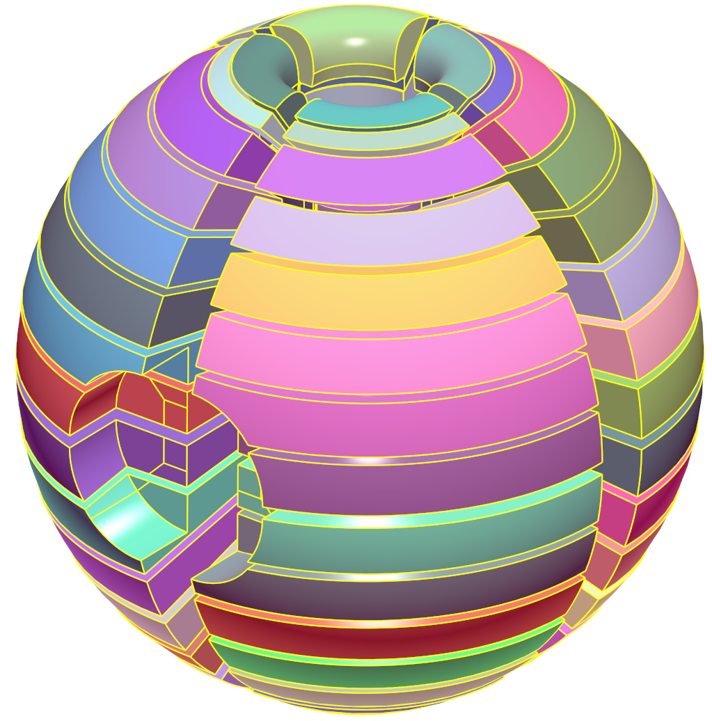    Figure 3: Subdivision of trimmed B-spline trivariates into trimmed Bézier trivariates. (a) Ten trimmed B-spline trivariates forming a spherical volumetric model. (b) Subdivision of the trimmed trivariates in (a) into 72 trimmed Bézier trivariates (an exploded view).

3.2 Untrimming a Bézier trimmed trivariate

In this section, we describe an algorithm to decompose a trimmed Bézier trivariate ${\cal T}$ into a set of possibly singular on the boundary tensor product B-spline trivariates that covers ${\cal T}$. Recall ${\cal T}$ is represented as a tensor product Bézier trivariate $T$, and a set of trimming (trimmed) B-spline surfaces, ${\cal S}$. The trimmed surfaces in ${\cal S}$ can be classified into two groups: The first group contains boundary surfaces of $T$ that are possibly trimmed, and the second group contains surfaces that are general trimming (trimmed) surfaces in the Euclidean space that can be, for example, a result of Boolean operation with other (trimmed) trivariate. Since we aim for IGA applications that require integration over the trimmed trivariate’s domain in the parametric space, the Euclidean space surfaces in ${\cal S}$ need to be back projected into the parametric domain of $T$. However, trimming surfaces in the second group can not, in general, have an algebraic form and can not have a precise piecewise-polynomial image in the parametric space of $T$. In such cases, the trimming surfaces must be approximated in the parametric space, for example, by a least squares fit.

Algorithm 3 describes the untrimming algorithm of a trimmed Bézier trivariate; decomposing a trimmed Bézier trivariate into a set of mutually exclusive (singular only on the boundary) tensor product B-spline trivariates $\tau$ that cover the trimmed parametric domain of ${\cal T}$, where $T(\tau)$ covers ${\cal T}$ in the Euclidean space. The key idea of the algorithm is finding a kernel point of ${\cal T}$: an internal point in ${\cal T}$ that is visible from all points on all trimming surfaces in ${\cal S}$. If such a kernel point, $P$, exists, the set of trimming (trimmed) surfaces of ${\cal T}$, ${\cal S}$, is untrimmed: ${\cal S}$ is decomposed into a set of tensor product B-spline surfaces, $\overline{{\cal S}}$, by surface untrimming operations, for example following Massarwi et al. [2018]. A singular (only on its boundary) tensor product B-spline trivariate is then constructed between $P$ and each surface in $\overline{{\cal S}}$. Alternatively, If no kernel point exists, ${\cal T}$ is subdivided along an iso parametric direction, and the algorithm is recursively applied on each part.

The algorithm suggests a solution for the 3D art-gallery Marzal [2012], Berg et al. [2008] for objects having free form (trimmed) boundary surfaces, where each kernel point can be treated as a guard. However, clearly, the algorithm is not optimal in terms of minimal number of kernel points. Finding the optimal solution of the art gallery problem, even for planar polygons, is NP-hard Lee and Lin [1986]

The algorithm is iterative; each iteration consists of four steps. In the first step, discussed in Section 3.2.1, ${\cal S}$ is untrimmed to tensor product B-spline surfaces, $\overline{{\cal S}}$ (see line 2 in Algorithm 3). In the second step, discussed in Section 3.2.2, the untrimmed tensor product surfaces from the previous step are approximated in the parametric space of $T$ (see line 3 in Algorithm 3). In the third step, discussed in Section 3.2.3, the algorithm seeks a kernel point in the domain of ${\cal T}$, and if such a kernel point is found, builds mutually exclusive tensor product trivariates that cover ${\cal T}$ (see lines 4-9 in Algorithm 3). In the fourth step, discussed in Section 3.2.4, if no kernel point is found, ${\cal T}$ is subdivided into several parts (using Algorithm 1), and the untrimming algorithm is recursively invoked on each part (see lines 11-15 in Algorithm 3). Section 3.2.4 also discusses the termination of this algorithm.

Input:
${\cal T}=\{T,{\cal S}\}$: a trimmed Bézier trivariate; $T$ is the tensor product Bézier trivariate, that is trimmed by set of trimmed surfaces ${\cal S}$; Output:
$\tau$: a set of mutually exclusive (singular only on the boundary) tensor product B-spline trivariates that covers the parametric domain of ${\cal T}$; Algorithm:

1:  $\tau$ := $\emptyset$;

2:  $\overline{{\cal S}}$ := Untrimming trimmed surfaces in ${\cal S}$ into tensor product surfaces; // i.e. Massarwi et al. [2018]

3:  $\overline{{\cal S}}^{T}$ := Approximation of $T^{-1}(\overline{{\cal S}})$;

4:  $p$ := Find a kernel point of $\overline{{\cal S}}^{T}$;

5:  if $p\neq null$ then

6:     for all $s_{i}(u,v)\in\overline{{\cal S}}^{T}$ do

7:        $U_{i}(u,v,w):=(1-w)p+ws_{i}(u,v),~{}w\in[0,1]$;

8:        $\tau:=\tau\bigcup\{U_{i}(u,v,w)\}$;

9:     end for

10:  else

11:     $t,dir$ := Find a subdivision parametric value $t$, for $T$, in direction $dir$;

12:     ${\cal T}_{t}^{dir}$ := TrimTrivarSubdiv(${\cal T}$, $t$, $dir$); //Algorithm 1

13:     for all ${\cal T}_{i}\in{\cal T}_{t}^{dir}$ do

14:        $\tau:=\tau\bigcup$ TrivBezierUntrim(${\cal T}_{i}$);

15:     end for

16:  end if

17:  return  $\tau$;

Algorithm 3 TrivBezierUntrim(${\cal T}$): Decomposing trimmed Bézier trivariate ${\cal T}$ into (singular only on the boundary) tensor product B-spline trivariates.

3.2.1 Untrimming of the trimming surfaces in ${\cal S}$

At each iteration of Algorithm 3, the trimming surfaces of ${\cal T}$, ${\cal S}$, which can be trimmed surfaces, are untrimmed in Euclidean space. In the process of untrimming trimmed surface $S_{i}\in{\cal S}$, $S_{i}$ is precisely decomposed into a set of tensor product B-spline surfaces that covers $S_{i}$. In this work, we use the minimal weight untrimming algorithm proposed in Massarwi et al. [2018]; though, any other untrimming algorithm of trimmed surfaces can be employed as well. The untrimming algorithm in  Massarwi et al. [2018] guarantees positive determinant of the Jacobian in the interior of the resulting tensor product surfaces, provided the input is regular. The untrimming of ${\cal S}$ is needed for the next steps since it simplifies the visibility test used in seeking a kernel point (see Section 3.2.3), as visibility test for a tensor product B-spline surface is simpler than the same test for a trimmed surface - where an intersection between trimming curves and the boundaries of the visible regions of the underlying tensor product surface should be computed.

3.2.2 Approximating ${\cal S}$ in the parametric space of $T$

After untrimming ${\cal S}$ into tensor product surfaces, $\overline{{\cal S}}$, as described in Section 3.2.1, each tensor product surface $\overline{S_{i}}\in\overline{{\cal S}}$ is least squares approximated with a tensor product surface $s_{i}$ in the parametric space of $T$, such that $\overline{S_{i}}\cong T(s_{i})$. The approximation parameters of $s_{i}$ are (in each parameter direction): The number of samples $m$ of $\overline{S_{i}}$, the order $o$ of $s_{i}$, and the number of control points, $n$, of $s_{i}$. The approximation algorithm consists of three steps:

1. Sample $m^{2}$ points on $\overline{S_{i}}$, $\{P_{jk}\}$.

2. For each sample $P_{jk}=P_{jk}(x,y,z)$, find the back projected point $p_{jk}(u,v,w)$ in the parametric space of $T$, such that $T(p_{jk})=P_{jk}$. This can be done by finding the solution of the following system of three equations and three unknowns $(u,v,w)$:

   $$T_{x}(u,v,w)=x,~{}~{}~{}~{}~{} T_{y}(u,v,w)=y,{}{}{}{}{} T_{z}(u,v,w)=z,$$ (2)

   where $T_{x},T_{y},T_{z}$ refer to the $x,y,z$ components of $T(u,v,w)$ respectively. Note that if $T$ is regular, only a single solution exists.

3. $s_{i}\leftarrow$ Least squares approximation Atkinson [2008] of $\{p_{jk}\}$, by a tensor product B-spline surface of size $(n\times n)$ and orders $(o\times o)$.

Quite a few methods exist for computing the precise (up to machine-precision) back projections of points in freeforms. This classic inverse problem is, for example, efficiently solved billions of times in Ezair and Elber [2017] for a regular trivariate $T(u,v,w)$ by posing it as (and solving) three algebraic constraints in $(u,v,w)$ (as in Equation (2)). Going from back projection of points to back projection of curves and surfaces is more involved but relates to fitting freeforms to point sets, methods that are well digested and are beyond the scope of this work.

The approximation process described above is applied only to surfaces that are not lying on the boundaries of $T$. In the case of a trimming surface that is a (trimmed) boundary surface of $T$, $s_{i}$ is simply extracted as that boundary. See an example in Figure 4. Finally, note $T(s_{i})$ can be precisely computed by a symbolic surface-trivariate composition DeRose et al. [1993], Elber [1992].

Figure 4: Untrimming and approximating trimming surfaces, ${\cal S}$, in the parametric space of trivariate $T$. (a) The trivariate $T$ in Euclidean space. (b) The trimming surfaces, ${\cal S}$, also in Euclidean space. (c) $\overline{\cal S}$, the untrimming of ${\cal S}$ in the Euclidean space. (d) Approximation of $\overline{\cal S}$ in the parametric space of $T$, by tensor product surfaces of orders 3x3.

3.2.3 Seeking a kernel point

A kernel point of a closed B-rep model is an internal point that is visible from every point on the boundary of the model Berg et al. [2008]. Consider the trimming surfaces of a trimmed trivariate, given as a set of tensor-product B-spline surfaces, $\overline{{\cal S}}^{T}$, (following the untrimming process in Section 3.2.1, and the back projection to the parametric space in Section 3.2.2).

Lemma 5.

Assume every surface $s_{i}\in\overline{{\cal S}}^{T}$ is $C^{1}$. A point $p$ is a kernel point of the B-rep bounded by $\overline{{\cal S}}^{T}$, if the following condition is satisfied:

$$\langle p-s_{i}(u,v),n_{i}(u,v))\rangle>0,\forall s_{i}\in\overline{{\cal S}}^{T},\forall u,v\in s_{i},$$ (3)

where $n_{i}(u,v)=\frac{\partial s_{i}}{\partial u}\times\frac{\partial s_{i}}{\partial v}$ is the (unnormalized) normal field of $s_{i}$, pointing into the B-rep. Again, note $s_{i}$ is regular in its interior and hence $n_{i}$ never vanishes in the interior of the domain.

Proof.

As stated at the beginning of Section 3, we assume $n_{i}(u,v)$ points inside ${\cal T}$. Under this assumption, an internal point $p$ is visible to a point on a surface $s_{i}(u,v)$, if the straight line segment between $p$ and $s_{i}(u,v)$ is in the positive half plane defined by the normal $n_{i}(u,v)$ and the point $s_{i}(u,v)$, meaning that the vector $p-s_{i}(u,v)$ and the normal $n_{i}(u,v)$ satisfy: $\langle p-s_{i}(u,v),n_{i}(u,v)\rangle>0$. Moreover, the line segment $\overline{p,s_{i}(u,v)}$ lies entirely inside ${\cal T}$.

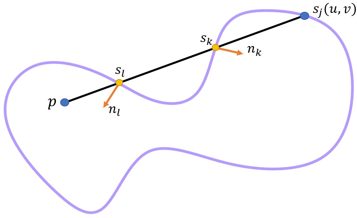
Now, given an internal point $p$ that satisfies Equation (3), and assume, by contradiction, that there exists a point $s_{j}(u,v)$ that is not visible to $p$. Examine the line segment $L=\overline{p,s_{j}(u,v)}$. Since $s_{j}(u,v)$ is not visible to $p$, then, by the Jordan-Brouwer separation theorem Lima [1988], and ignoring tangential contact(s) for now, there exists a finite segment of $L$ that lies entirely outside ${\cal T}$. Otherwise, if $L$ is entirely inside ${\cal T}$, then $s_{j}(u,v)$ is visible to $p$. Let $\overline{s_{l},s_{k}}$ be the segment of $L$ that is outside ${\cal T}$, where $s_{l}$ is the closest point to $p$ (See illustration on Figure 6). Because, $\overline{s_{l},s_{k}}$ stabs the boundary at $s_{k}$ from outside, $\langle p-s_{k},n_{k}\rangle$ can not be positive, contradicting the assumption that $p$ satisfies Equation (3), for all $s_{i}$. With special care, and following similar lines, one can also handle tangential contacts. ∎

Figure 5: Auxiliary illustration for Lemma 5.

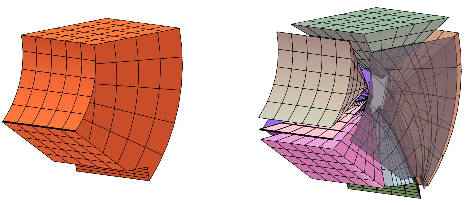    Figure 6: Untrimming of a trimmed Bézier trivariate, after finding a kernel point. A trimmed rational Bézier trivariate of orders (4,2,2) having nine trimming trimmed surfaces in (a). Once a kernel point is found, nine (singular on the boundary) tensor product trivariates are constructed (b), and shown in an exploded view.

Lemma 5 states that if all surfaces $s_{i}\in\overline{{\cal S}}^{T}$ are front facing with respect to $p$, then all $s_{i}\in\overline{{\cal S}}^{T}$ are visible to $p$, in a similar way to front face visibility in projections, in graphics.

Note that although the normal of the entire closed B-rep bounded by $\overline{{\cal S}}^{T}$ is not defined on intersection/stitching $C^{0}$ points between surfaces in $\overline{{\cal S}}^{T}$, the proof is still valid on such points, as Equation (3) still holds for each $s_{i}$ surface.

More details on freeform surface visibility can be found in Elber and Cohen [1995]. Equation (3) can be computed by symbolically representing this inner product  Elber [1992] as a tensor product B-spline function, and verifying the positivity of all the control coefficients.

As a side comment, the kernel, if any, can be bound using an approach that utilizes the intersections of all tangent planes at all parabolic points of $\overline{{\cal S}}$, assumed $C^{2}$ Cohen et al. [2002]. However, such an approach, that involves computing parabolic points, is computationally expensive and numerically challenging. Instead, and since herein we only seek a single kernel location, the trimmed parametric domain of ${\cal T}$ is uniformly sampled, and the visibility test of Equation (3) is verified on each sample. There could be more than one kernel sample that satisfies Equation (3). Among these samples, we, heuristically, pick the kernel point as the sample, $p$, that minimizes the following expression:

$$\max_{\forall s_{i}\in\overline{{\cal S}}^{T}}{(\min_{u,v}(\lVert s_{i}(u,v)-p\rVert))}-\min_{\forall s_{j}\in\overline{{\cal S}}^{T}}{(\min_{u,v}(\lVert s_{j}(u,v)-p\rVert))},$$ (4)

that promotes kernel points for which the deviations of the maximal and minimal distance to the boundaries are minimal, as we try to avoid thin and tall trivariates in the output, as much as possible.

During the process of seeking a kernel point, as only $p$ changes during the domain sampling, caching computation results that are independent of $p$, such as $\langle s_{i}(u,v),n_{i}(u,v)\rangle$ in Equation (3), will result in a significant speed up improvement.

If a kernel point $p$ is found, a tensor product B-spline trivariate $U_{i}(u,v,w)$ is constructed as a singular ruled trivariate Cohen et al. [2002] between $p$ and each tensor product B-spline surface $s_{i}(u,v)\in\overline{{\cal S}}^{T}$, as following:

$$U_{i}(u,v,w)=(1-w)p+ws_{i}(u,v),w\in[0,1].$$ (5)

Since $s_{i}(u,v)$ is guaranteed to (possibly) have singularities only on the boundaries (property of the surfaces’ untrimming algorithm Massarwi et al. [2018]), so is $U_{i}(u,v,w)$. See an example of untrimming of a trimmed Bézier trivariate in Figure 6.

Note that although the trimming curves are typically the result of Boolean set operations, and hence piecewise linear, the algorithm can handle smooth trimming curves of arbitrary order. The trivariates’ construction procedures can handle higher order curves as is. However, a B-spline curve fitting process needs to be applied in the back projection approximation in the parametric space, as discussed in Section 3.2.2.

3.2.4 Subdivision of ${\cal T}$

At each iteration, if no kernel point is found, ${\cal T}$ is subdivided into several trimmed trivariates, and the untrimming algorithm is recursively applied on each part. Several strategies can be utilized to choose the subdivision direction and value. In this work, the subdivision is performed, using Algorithm 1, along the center of the bounding box of ${\cal T}$, in the parametric space, and the parametric direction is the direction of the longest dimension of the bounding box. This strategy ensure that the trimmed domain is getting smaller with each iteration.

During the iterative subdivision process, a non-trimmed (full tensor product) trivariate domains can be obtained, having six tensor product isoparametric boundary surfaces. In such cases, there is obviously no need to compute a kernel point and the trivariate is not subdivided further. Further, during the subdivision process, not all boundary surfaces are subdivided, in practice, in each iteration. Hence, we cache the untrimming and approximation results of the surfaces (results of steps 2 and 3 in Algorithm 3, respectively) to be used in forthcoming iterations.

We consider a special case that is handled differently: If the size of $s_{i}$, and the aperture of the normal cone of $s_{i}$ for each trimming surface, $s_{i}\in{\overline{\cal S}}^{T}$, is less than a predefined thresholds $\epsilon_{e}$ and $\epsilon_{\theta}$ respectively, then each $s_{i}$ is approximated by a planar surface, resulting in a polyhedron, $C$, that approximates ${\overline{\cal S}}^{T}$. Then, kernel points of $C$ can always be found, following  Marzal [2012] for example.

Lemma 6.

Assume all surfaces $s_{i}\in{\overline{\cal S}}^{T}$ have a bounded curvature. If the subdivision process satisfies the following:

• The subdivision is performed at the center of the bounding box of ${\cal T}$ along the direction of the longest dimension of the bounding box, and,

• ${\overline{\cal S}}^{T}$ is approximated by a polyhedron when the size of each $s_{i}\in{\overline{\cal S}}^{T}$ and the aperture of the normal cone of each $s_{i}\in{\overline{\cal S}}^{T}$, is less than a predefined thresholds, $\epsilon_{e}$ and $\epsilon_{\theta}$, respectively,

then, Algorithm 3 terminates after a finite number of iterations.

Proof.

Each surface $s_{i}\in{\overline{\cal S}}^{T}$ is represented as a B-spline surface, and $s_{i}$ has a bounded curvature, by assumption. In other words, for each threshold $\epsilon_{\theta}$, there exists a threshold $\epsilon_{e}$ such that if the size of $s_{i}$ is less than $\epsilon_{e}$ (which can be achieved by a finite number of subdivisions), then the aperture of the normal cone of $s_{i}$ is less than $\epsilon_{\theta}$. Since the subdivision is performed along the longest dimension, it is guaranteed that the size of $s_{i}$ is getting smaller at each iteration.

Eventually, after a finite number of iterations, and if no kernel point is found, the size of each surface $s_{i}$ will be less than $\epsilon_{e}$ and the aperture of the normal cone of $s_{i}$ will be less than $\epsilon_{\theta}$. At that iteration, ${\overline{\cal S}}$ is approximated by a polyhedron and the algorithm terminates. ∎

4 Results

The algorithms presented in this paper are all implemented in the IRIT Elber [2015] solid modeling kernel. We now present results of the untrimming algorithm applied on several trimmed trivariates and V-rep models. The following examples were synthesized on a 3.4 GHz Intel i7 CPU with 32 GB RAM in a single thread mode and Windows 7. Practically, in all the examples presented in this paper, we never failed to find a kernel point and never had to resort to the polyhedron approximation (Recall Section 3.2.4).

Model	Input		Output
	# Trimmed	# Trimming	# Tensor	# Total	Maximal	Total	(E)uclidean
	trivariates	surfaces	product	domain	subdivision	time	or
			Trivariates	subdivisions	depth	(Sec.)	(P)arametric
Figure 7	1	11	262	30	9	251	P
Figure 8	1	24	76	5	3	52	P
Figure 10	1	24	406	13	5	10.5	E
Figure 10	7	64	294	32	7	13.2	E
Figure 12	20	168	370	22	4	20.9	E
Figure 12	1	34	56	3	2	2.9	E

Table 1: Statistics on the process of untrimming the trimmed trivariates presented in Figures 7-12.

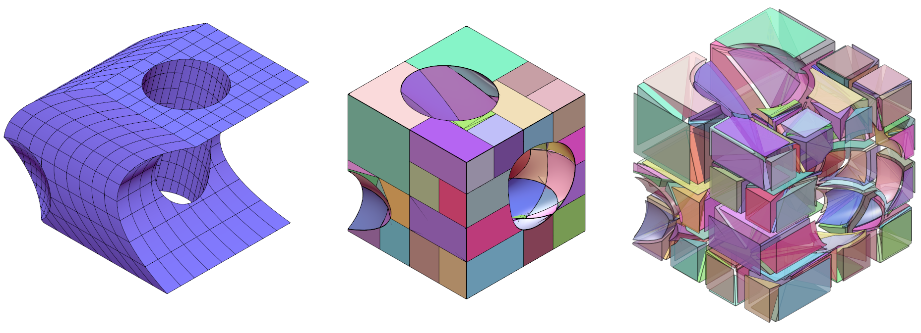
Figure 7 shows the result of untrimming a trimmed Bézier trivariate of orders (2,2,3). The untrimming is performed in the parametric space, and the trimming surfaces are untrimmed and approximated by a set of bi-quadratic surfaces. The result consists of 262 tensor product B-spline trivariates that covers the trimmed parametric domain of the trimmed trivariate. The whole untrimming process took 251 seconds, out of which the approximation of the untrimmed surfaces in the parametric space took 107 seconds.

Figure 7: Untrimming of a trimmed Bézier trivariate. (a) A trimmed Bézier trivariate of orders (2,2,3). (b) Untrimming result in the parametric space of (a), yielding 262 tensor product B-spline trivariates shown in an exploded semi-transparent view in (c).

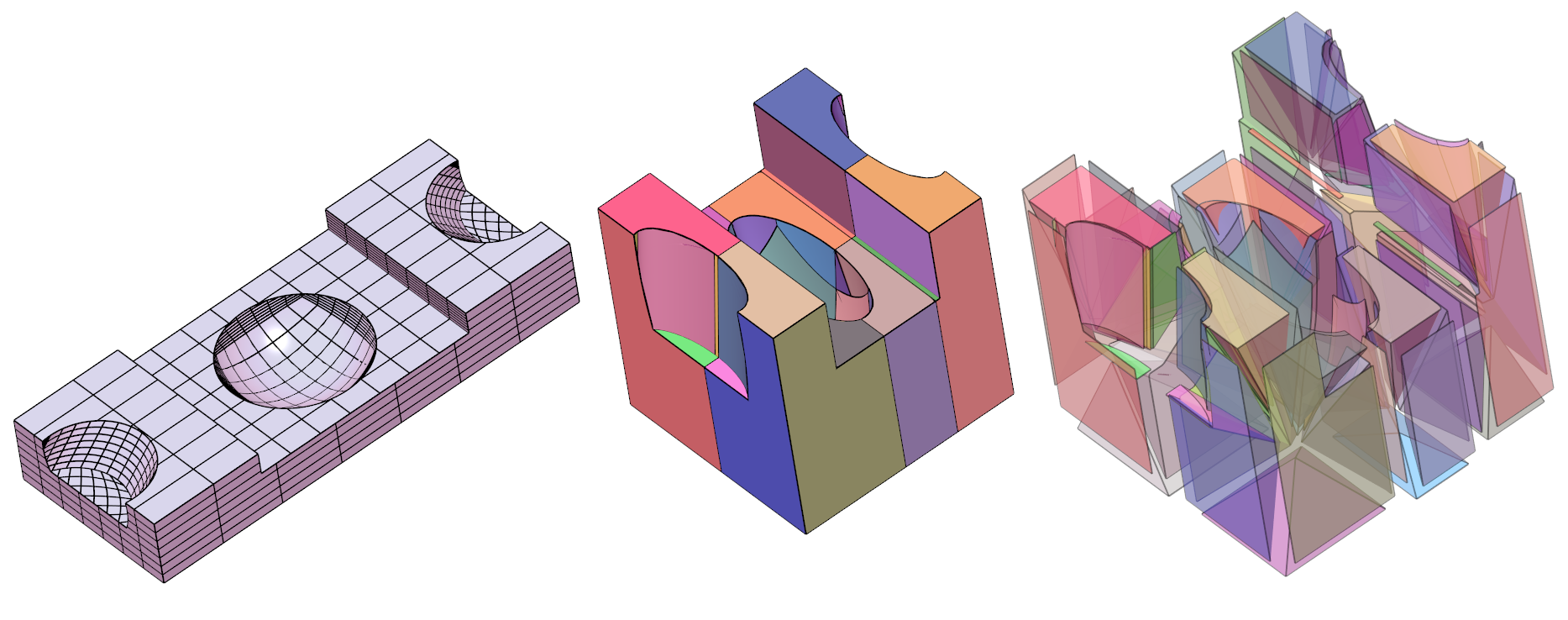
In Figure 8, a V-rep model consisting of one trimmed trilinear trivariate is untrimmed in the parametric space, resulting in 76 tensor product trivariates that cover the trimmed parametric domain of the model. The trimming surfaces are untrimmed and approximated by bi-quadratic surfaces in the parametric domain. The untrimming algorithm took 52 seconds, out of which the approximation of the untrimmed surfaces in the parametric domain took 33 seconds.

Figure 8: Untrimming of a V-model. (a) The trimmed trivariate of the V-model. Untrimming result consisting of 76 tensor product B-spline trivariates composing the parametric domain in (b) and shown in semi-transparent exploded view in (c).

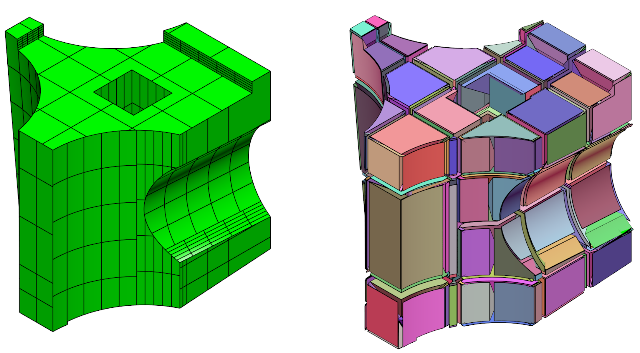
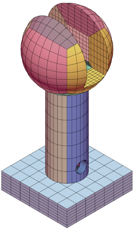
Figure 10 shows untrimming of a complex trimmed trilinear B-spline trivariate having (4,4,3) internal Bézier domains. The untrimming is performed in the Euclidean space, resulting in 406 tensor product B-spline trivariates. The trimmed trivariate is first subdivided at all internal knots into 42 trimmed Bézier trivariates (and not $48=4\times 4\times 3$, as some domains are completely trimmed away), and then each trimmed Bézier trivariate is untrimmed into a set of tensor product B-spline trivariates. The untrimming process took 10.5 seconds, out of which the subdivision of the trimmed trivariate into trimmed Bézier trivariates took 1.1 seconds.

Figure 9: Untrimming of a trilinear trimmed B-spline trivariate with ($4\times 4\times 3$) Bézier domains. (a) The trimmed B-spline trilinear trivariate. (b) Untrimming of (a) yielding 406 tensor product B-spline trivariates displayed in an exploded view.

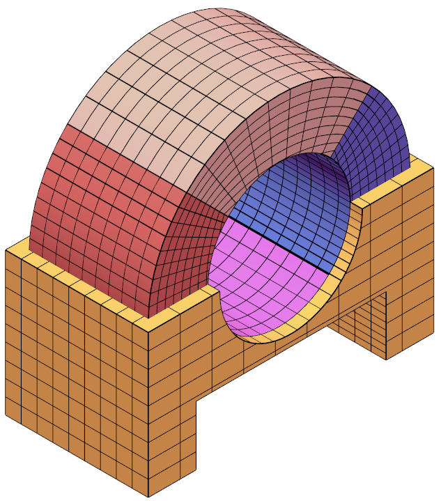
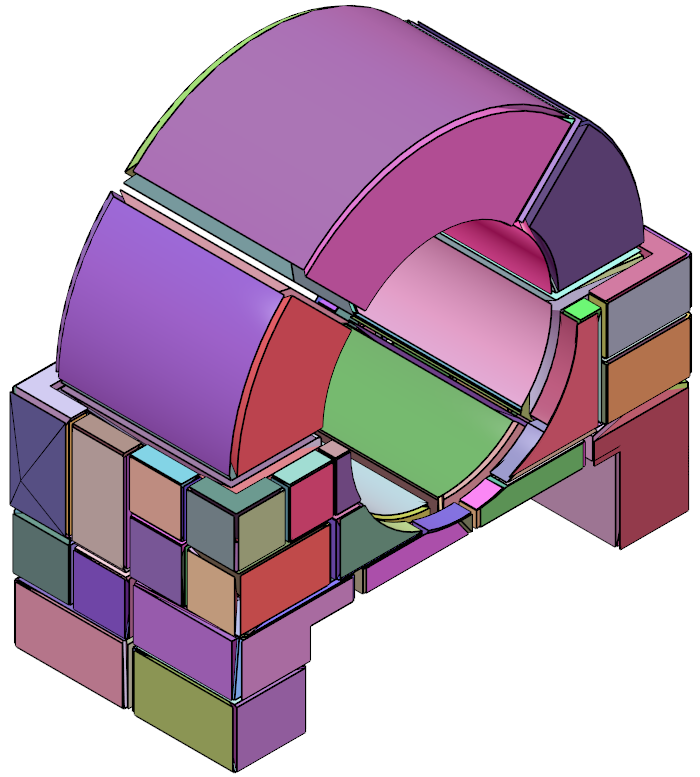    Figure 10: Untrimming of a V-model. (a) The V-model consisting of seven trimmed trivariates. (b) The result of untrimming each of the trimmed trivariates of the model, resulting in 294 tensor product B-spline trivariates displayed in an exploded view.

Figures 10 and 12 show two untrimming results of volumetric models (V-models). Each V-model consists of several trimmed trivariates. Since the trimmed trivariates do not share the same parametric space, and in order to emphasize how the untrimming result covers the entire V-model, the untrimming is performed in the Euclidean space. In Figure 10, the V-model, consisting of seven mutually exclusive trimmed trivariates, is untrimmed in 13.2 seconds, resulting in 294 tensor product B-spline trivariates. In Figure 12, another V-model, consisting of 20 mutually exclusive trimmed trivariates, is untrimmed in 20.9 seconds, resulting in 370 tensor product B-spline trivariates.

Figure 11: Untrimming of a V-model. (a) The V-model consisting of 20 trimmed trivariates. (b) The result of untrimming each of the trimmed trivariates of the model, resulting in 370 tensor product B-spline trivariates displayed in an exploded view.

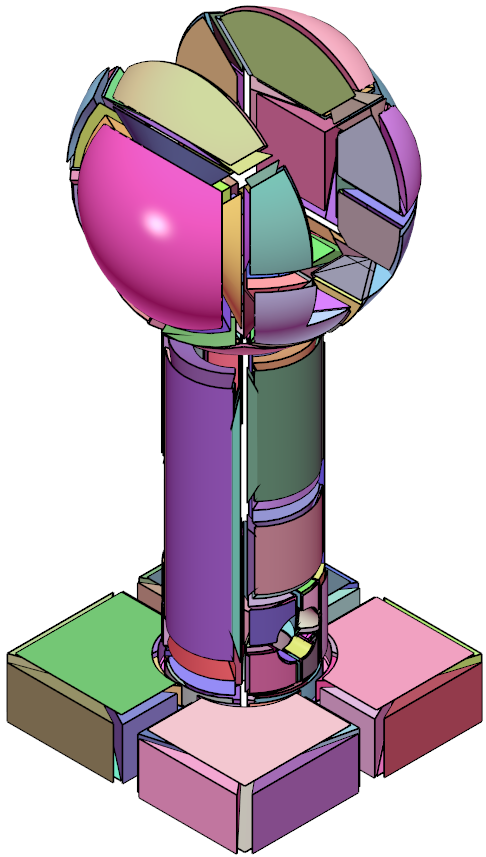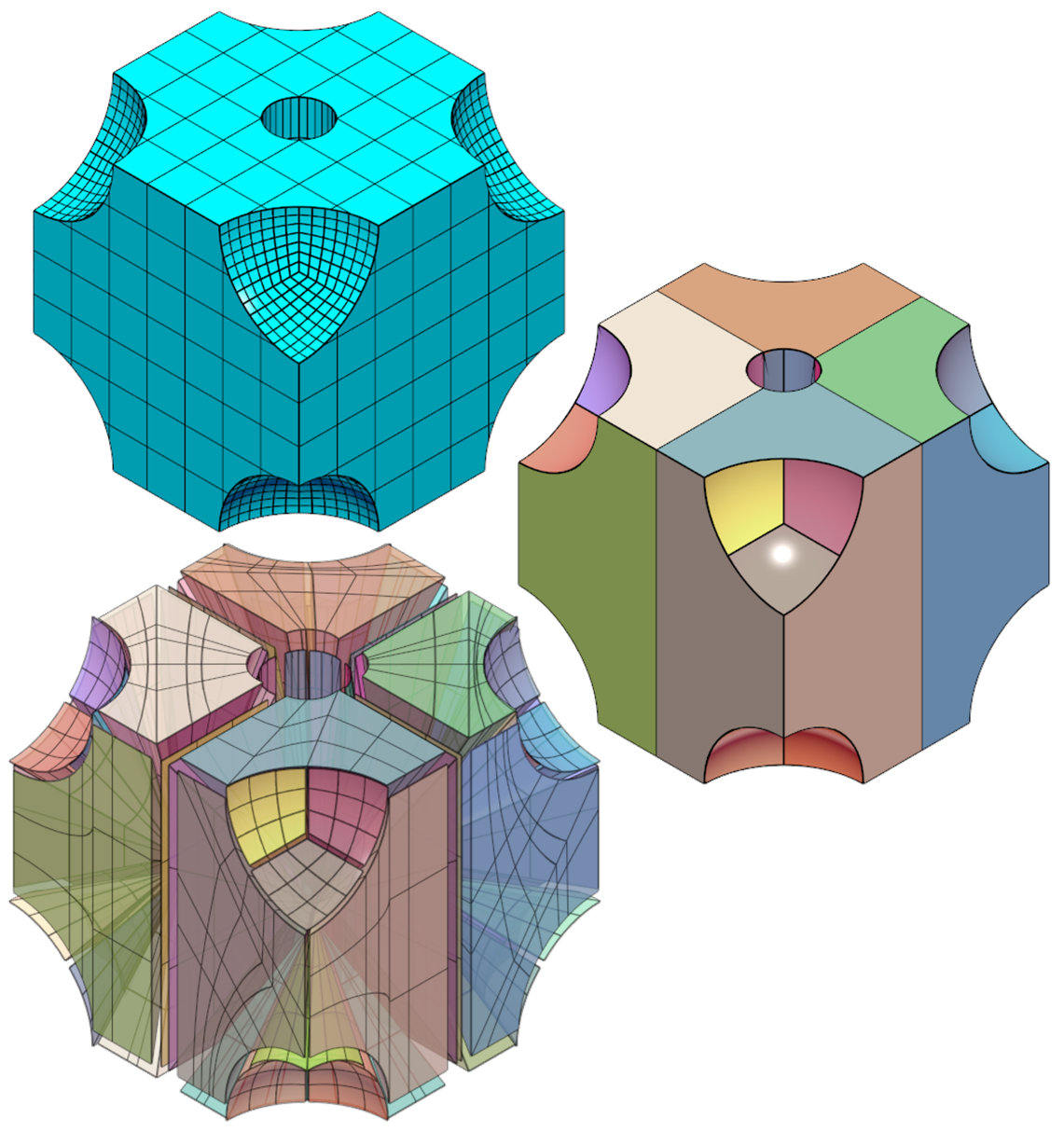  Figure 12: (a) A trimmed trivariate constructed by subtracting from a unit cube eight spheres of radius 0.3 centered at the eight corners of the cube, and a cylinder of radius 0.1 from the center of the cube. (b) Untrimming of (a) results in 56 tensor products that are displayed in an exploded view in (c).

Precise computation of integral properties over trimmed trivariates are more difficult than over tensor products. In Figure 12, we show one application of the untrimming algorithm. We precisely compute the trimmed trivariate’s volume by first untrimming the trimmed trivariate into tensor products, and then computing the volume of all covering tensor products. Since we use symbolic spline integration Elber [1992], the geometry must be (piecewise) polynomial (and not rational). Hence, arcs and circles are approximated using piecewise polynomials to an accuracy of ${\sim}10^{-3}$. The object in Figure 12(a) is constructed by subtracting the following from a unit cube: (i) eight spheres of radii 0.3 centered at the corners of the cube, and (ii) a cylinder with a radius of 0.1 along the center of the unit cube. The analytic value of the trimmed cube’s volume is 0.855486. While the value we compute is 0.855284, a result that is well within the arc approximation.

Finally, some statistics on the untrimming process (Algorithm 3) of the trimmed trivariates in Figures 7-12 are presented in Table 1. In the input part, the number of trimmed trivariates in each model and the number of total trimming surfaces for all the trimmed trivariates are presented in the first and the second columns respectively. In the output section, the first column shows the number of tensor product trivariates in the result of the untrimming algorithm. The second column shows the total number of subdivisions of the domain performed during the untrimming process. The third column shows the maximal depth of the recursive subdivision calls, in the untrimming algorithm. The fourth column shows the total running time, in seconds, and the last column indicates if the untrimming is done in the parametric space or in the Euclidean space.

5 Analysis using untrimmed trivariates

In this section, we illustrate the use of the presented untrimming methodology for performing isogeometric analysis in domains defined with trimmed B-spline trivariates. As a matter of example we focus in this section on a linear elasticity problem setting, that is governed by the variational equation:

$$\int_{\mathcal{T}}\mu(\bm{x})\nabla^{s}\bm{u}(\bm{x}):\nabla^{s}\bm{v}(\bm{x})\text{d}\bm{x}+\int_{\mathcal{T}}\lambda(\bm{x})\nabla\cdot\bm{u}(\bm{x})\,\nabla\cdot\bm{v}(\bm{x})\text{d}\bm{x}=\int_{\mathcal{T}}\bm{f}(\bm{x})\cdot\bm{v}(\bm{x})\text{d}\bm{x}+\int_{\mathcal{S}_{N}}\bm{g}(\bm{x})\cdot\bm{v}(\bm{x})\text{d}\bm{x},$$ (6)

where $\bm{u}:\mathcal{T}\to\mathbb{R}^{3}$ is the elastic displacement at every point of the domain, the problem unknown, and $\bm{v}:\mathcal{T}\to\mathbb{R}^{3}$ corresponds to the test functions. On the other hand $\bm{f}:\mathcal{T}\to\mathbb{R}^{3}$ and $\bm{g}:\mathcal{S}_{N}\to\mathbb{R}^{3}$ are the volumetric forces (e.g. self-weight) and the external loads applied on the external boundary (e.g. pressure). $\mathcal{S}_{N}$ is a subset of the exterior boundary $\mathcal{S}$ in which external loads are applied. Finally, $\lambda$ and $\mu$ are the Lamé parameters that charaterize the behaviour of the elastic material, that may change from point to point. For the sake of brevity, prescribed displacements (Dirichlet boundary conditions) are not discussed here. In an IGA context, both $\bm{u}$ and $\bm{v}$ are discretized by means of trivariate B-splines:

$$\bm{u}=\sum_{i=0}^{l}\sum_{j=0}^{m}\sum_{k=0}^{n}\bm{u}_{i,j,k}B_{i,d_{u}}(u)B_{j,d_{v}}(v)B_{k,d_{w}}(w),$$ (7)

where the coefficients $\bm{u}_{i,j,k}\in\mathbb{R}^{3}$ are the problem unknowns ($\bm{v}$ is discretized in the same way). We refer the interested readers to Cottrell et al. [2009] for a more detailed discussion about the fundamentals of IGA. Thus, in an isoparametric framework we use the same spline space for describing both the trivariate $T$ (as in Equation (1)) and discretizing the solution (trial) $\bm{u}$ and the test functions $\bm{v}$. For the analysis, the support of functions $B_{i,d_{u}}$, $B_{j,d_{v}}$, $B_{k,d_{w}}$ is limited to the active region of the domain defined by the trimming. Therefore, those functions whose support is completely outside of the trimmed domain will not be considered in the analysis.

In order to compute the integrals present in the Equation (6) in the domain $\mathcal{T}$ (and on the boundary $\mathcal{S}_{N}$) we decompose the integral over the full domain as the sum of the integrals in every single Bézier element contained in the domain. Thus, for computing the integral of a generic quantity $\alpha(\bm{x})$ over the domain $\mathcal{T}$ we split the integral as: $\int_{\mathcal{T}}\alpha(\bm{x})\text{d}\bm{x}=\sum^{n_{b}}_{i}\int_{\hat{\mathcal{B}_{i}}}\hat{\alpha}(\bm{x})\text{d}\bm{x}$, where $\hat{\mathcal{B}_{i}}$ are the representation, in the parametric domain of $T$, of the trimmed Bézier trivariates $\mathcal{B}_{i}$ (such that $\mathcal{T}=\cup^{n_{b}}_{i}\mathcal{B}_{i}$), and $n_{b}$ is the number of trivariates. $\hat{\alpha}(\bm{x})$ corresponds the pull-back of $\alpha(\bm{x})$. Thus, when computing $\int_{\hat{\mathcal{B}_{i}}}\hat{\alpha}(\bm{x})\text{d}\bm{x}$ for $i=1,\dots,n_{b}$ there exist two possible situations:

• If $\hat{\mathcal{B}_{i}}$ is not a trimmed trivariate, but a full one, then a Gaussian quadrature rule is applied for computing the integral. This is the case of standard IGA methods for non-trimmed domains.

• Otherwise, if $\hat{\mathcal{B}_{i}}$ is a trimmed trivariate, the element is untrimmed according to methodology presented in Section 3, and the integral is computed using the resulting untrimming trivariates as:

  $$\int_{\hat{\mathcal{B}_{i}}}\hat{\alpha}(\bm{x})\text{d}\bm{x}=\sum^{n_{u,i}}_{j=1}\int_{\tau_{i,j}}\hat{\alpha}(\bm{x})\text{d}\bm{x},\qquad\textrm{for }i=1,\dots,n_{b},$$ (8)

  where $\tau_{i,j}$ is the $j$-th untrimming tensor product trivariate of the Bézier element $\hat{\mathcal{B}_{i}}$, with $j=1,\dots,n_{u,i}$.

A discussion regarding the integration of the trimmed and non-trimmed Bézier elements can be found in Rank et al. [2012]. It is important to remark here that the tensor product trivariates $\tau_{i,j}$ are only used for integration purposes. Therefore, they are not required to have high-quality Jacobians, and it is sufficient that they are singular only on their boundary.

Remark 7.

To perform analyses, in an IGA framework, in the case of computational domains created as the union of more than one trimmed B-spline trivariate (e.g. Figures 10 and 12) is not as straightforward as for single trimmed trivariates. These situations involve not only the precise integration of the operators described in Equation (6), but also the consistent gluing of all the partial solution discretizations, defined for every single trivariate, in the intersection regions. The treatment of this kind of domains is out of the scope of this paper.

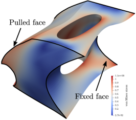
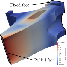
In order to illustrate the potentiality of the presented procedure, we perform linear elasticity numerical experiments for the trimmed geometries shown in Figures 7, 10 and 12.

The same elastic material is considered in all cases, being the Young modulus and the Poisson ratio, $E=1\,\text{MPa}$ and $\nu=0.3$, respectively (where $\lambda=E\nu/(1+\nu)(1-2\nu)$ and $\mu=E/2(1+\nu)$). The analysis were performed using the IGA library igatools described in Pauletti et al. [2015].

All three cases present analogous loading conditions: one face is completely fixed (no displacement in any direction is allowed) while the opposite face is pulled perpendicularly (the pulled face is free to deform transversally). In these cases, Dirichlet boundary conditions are applied on faces of $T$ (that could potentially be trimmed) in a strong way: the degrees of freedom associated to the basis functions whose traces have support on those faces are prescribed. On the other hand, the imposition of Dirichlet boundary conditions on trimming boundaries (that are not faces of $T$) requires the use of weak imposition methods. This is out of the scope of this paper, however, we refer the interested reader to Ruess et al. [2013] and Buffa et al. [2019], and references therein.

In Figure 13, we gathered some of the obtained results.

Figure 13: Linear elasticity analyses on trimmed geometries from Figures  7, 10 and 12. The von Mises stress distribution is plotted on the deformed geometries submitted to external loads: one face is fixed while the opposite face is pulled perpendicularly.

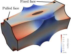The shown geometries are deformed with respect to the original ones as a consequence of the applied loads. The plotted (colored) scalar field corresponds the distribution of the von Mises stress.

The cases 13(a), 13(b) and 13(c) were obtained using trimmed B-spline trivariates with $(3\times 3\times 3)$, $(4\times 4\times 3)$ and $(4\times 4\times 4)$ Bézier domains, respectively, and discretizing the elastic displacement solutions with degree $2$ in every direction (i.e. the models have $375$, $540$ and $648$ degrees of freedom, respectively). Note that the models in Figures 7 and 12 have underlying Bézier trivariates, and in order to obtain a more precise analysis solution, the trivariates of these models were refined in each parametric direction. The computational times for the assembly of the stiffness matrices are $114$, $32$ and $61$ seconds, respectively; and the resolution of the linear system of equations took less than one second in all cases. The current untrimming process creates very accurate reparametrization of the trimmed domains. Nevertheless, from the analysis point of view such level of accuracy is not needed for integration purposes. Therefore, by creating much coarser reparametrizations the computational time of the matrix assembly could potentially be reduced by orders of magnitude.

6 Conclusion

In this work, an untrimming algorithm for trimmed trivariate is introduced: decomposing a trimmed B-spline trivariate into a set of mutually exclusive tensor product B-spline trivariates that completely cover the trimmed domain. The algorithm uses a subdivision algorithm, introduced in this paper, that precisely subdivides the trimmed B-spline trivariate into set of trimmed Bézier trivariates. The untrimming algorithm then generates tensor product B-spline trivariates that are singular only on the boundaries and thus can be utilized for integration in IGA application (i.e at quadrature locations). The quality of the analysis solution is not influenced by the Jacobians’ quality of the generated tensor product trivariates.

Several directions for further improvements can be sought. Additional strategies of selecting the subdivision location, in case no kernel point is found (see Section 3.2.4), can be further investigated, in order to minimize the number of subdivisions required and thus minimizing the number of generated trivariates in the output. For example, subdivision at locations that isolate individual non isoparametric trimming surfaces, if exist. That is, every trimmed trivariate will have at most one non iso-parametric trimming surface.

Aiming for less subdivisions when seeking the kernel points (see Section 3.2.3), one can explore better sampling approaches than the uniform sampling approach taken here. Similarly, a more precise (less lossy) approach can be sought, by computing a tight bounding box of the solutions of Equation (3) in Lemma 5, for all trimming surfaces, simultaneously. However, it requires the (simultaneous) processing of multiple bivariate inequalities (one for each trimming surface). While potentially possible, for example, using interval arithmetic, it can be time consuming.

Due to the independent untrimming of adjacent boundary surfaces, adjacent tensor product trivariates in the output might not share the same functional space, which makes the presented approach less suitable for other analysis approaches, such as domain decomposition Toselli and Widlund [2004], where constraints are imposed on shared boundaries. In order to have adjacent surfaces with the same functional space, the (trimmed) surfaces untrimming process (see Section 3.2.1) needs to be adapted to consider not only a single trimmed surface, but also the adjacencies between the trimming (trimmed) surfaces of the trivariate.

The back projection approximation process of trimming surfaces, in the parametric space, as described in Section 3.2.2, doesn’t guarantee stitched boundaries between adjacent surfaces, which likely to lead to black holes in the approximated surfaces that may introduce inaccuracies when using the untrimming results in applications, such as analysis. To overcome this limitation, the topological adjacency information should be provided to the back projection process, and proper stitching methods should be considered.

References

- Armstrong et al. [2015] Armstrong, C.G., Fogg, H.J., Tierney, C.M., Robinson, T.T., 2015. Common themes in multi-block structured quad/hex mesh generation. Procedia Engineering 124, 70–82.
- Atkinson [2008] Atkinson, K.E., 2008. An introduction to numerical analysis. John Wiley & Sons.
- Bartoň et al. [2017] Bartoň, M., Puzyrev, V., Deng, Q., Calo, V., 2017. Efficient mass and stiffness matrix assembly via weighted gaussian quadrature rules for b-splines. arXiv preprint arXiv:1710.01048 .
- Berg et al. [2008] Berg, M.d., Cheong, O., Kreveld, M.v., Overmars, M., 2008. Computational geometry: algorithms and applications. Springer-Verlag TELOS.
- Buffa et al. [2019] Buffa, A., Puppi, R., Vázquez, R., 2019. A minimal stabilization procedure for Isogeometric methods on trimmed geometries. arXiv:1902.04937 [math] URL: http://arxiv.org/abs/1902.04937. arXiv: 1902.04937.
- Cohen et al. [2002] Cohen, E., Riesenfeld, R., Elber, G., 2002. Geometric modeling with splines: An introduction. 2002. AK Peters Natick, MA, USA .
- Cottrell et al. [2009] Cottrell, J.A., Hughes, T.J., Bazilevs, Y., 2009. Isogeometric analysis: toward integration of CAD and FEA. John Wiley & Sons.
- DeRose et al. [1993] DeRose, T., Goldman, R., Hagen, H., Mann, S., 1993. Functional composition via blossoming. ACM Transactions on Graphics 12, 113–135.
- Elber [1992] Elber, G., 1992. Free Form Surface Analysis using a Hybrid of Symbolic and Numeric Computation. Ph.D. thesis. University of Utah.
- Elber [2015] Elber, G., 2015. Irit 11 user’s manual URL: http://www.cs.technion.ac.il/$∼$irit.
- Elber and Cohen [1995] Elber, G., Cohen, E., 1995. Arbitrarily precise computation of gauss maps and visibility sets for freeform surfaces, in: Proceedings of the third ACM symposium on Solid modeling and applications, ACM. pp. 271–279.
- Engvall and Evans [2017] Engvall, L., Evans, J.A., 2017. Isogeometric unstructured tetrahedral and mixed-element bernstein?bézier discretizations. Computer Methods in Applied Mechanics and Engineering 319, 83 – 123.
- Ezair and Elber [2017] Ezair, B., Elber, G., 2017. Fabricating functionally graded material objects using trimmed trivariate volumetric representations, in: Proceedings of SMI’2017 Fabrication and Sculpting Event (FASE), Berkeley, CA, USA.
- Geuzaine and Remacle [2009] Geuzaine, C., Remacle, J.F., 2009. Gmsh: A 3-d finite element mesh generator with built-in pre-and post-processing facilities. International journal for numerical methods in engineering 79, 1309–1331.
- Grandine and Klein [1997] Grandine, T.A., Klein, F.W., 1997. A new approach to the surface intersection problem. Computer Aided Geometric Design 14, 111 – 134. URL: http://www.sciencedirect.com/science/article/pii/S0167839696000246, doi:https://doi.org/10.1016/S0167-8396(96)00024-6.
- Lee and Lin [1986] Lee, D., Lin, A., 1986. Computational complexity of art gallery problems. IEEE Transactions on Information Theory 32, 276–282.
- Lima [1988] Lima, E.L., 1988. The jordan-brouwer separation theorem for smooth hypersurfaces. The American Mathematical Monthly 95, 39–42.
- Liu et al. [2014] Liu, L., Zhang, Y., Hughes, T.J., Scott, M.A., Sederberg, T.W., 2014. Volumetric t-spline construction using boolean operations. Engineering with Computers 30, 425–439.
- Martin and Cohen [2010] Martin, T., Cohen, E., 2010. Volumetric parameterization of complex objects by respecting multiple materials. Computers & Graphics 34, 187 – 197. Shape Modelling International (SMI) Conference 2010.
- Marussig and Hughes [2018] Marussig, B., Hughes, T.J.R., 2018. A review of trimming in isogeometric analysis: Challenges, data exchange and simulation aspects. Archives of Computational Methods in Engineering 25, 1059–1127. URL: https://doi.org/10.1007/s11831-017-9220-9, doi:10.1007/s11831-017-9220-9.
- Marzal [2012] Marzal, J., 2012. The three-dimensional art gallery problem and its solutions. Ph.D. thesis. Murdoch University.
- Massarwi and Elber [2016] Massarwi, F., Elber, G., 2016. A B-spline based framework for volumetric object modeling. Computer-Aided Design 78, 36 – 47. SPM 2016.
- Massarwi et al. [2018] Massarwi, F., van Sosin, B., Elber, G., 2018. Untrimming: Precise conversion of trimmed-surfaces to tensor-product surfaces. Computers & Graphics 70, 80–91.
- Pauletti et al. [2015] Pauletti, M.S., Martinelli, M., Cavallini, N., Antolin, P., 2015. Igatools: An isogeometric analysis library. SIAM Journal of Scientific Computing 37, 465 – 496.
- Rank et al. [2012] Rank, E., Ruess, M., Kollmannsberger, S., Schillinger, D., Düster, A., 2012. Geometric modeling, isogeometric analysis and the finite cell method. Computer Methods in Applied Mechanics and Engineering 249-252, 104 – 115. URL: http://www.sciencedirect.com/science/article/pii/S0045782512001855, doi:https://doi.org/10.1016/j.cma.2012.05.022. higher Order Finite Element and Isogeometric Methods.
- Ruess et al. [2013] Ruess, M., Schillinger, D., Bazilevs, Y., Varduhn, V., Rank, E., 2013. Weakly enforced essential boundary conditions for NURBS-embedded and trimmed NURBS geometries on the basis of the finite cell method. International Journal for Numerical Methods in Engineering 95, 811–846. URL: https://onlinelibrary.wiley.com/doi/full/10.1002/nme.4522, doi:10.1002/nme.4522.
- Satoh and Chiyokura [1991] Satoh, T., Chiyokura, H., 1991. Boolean operations on sets using surface data, in: Proceedings of the First ACM Symposium on Solid Modeling Foundations and CAD/CAM Applications, ACM, New York, NY, USA. pp. 119–126. URL: http://doi.acm.org/10.1145/112515.112536, doi:10.1145/112515.112536.
- Thomas [1986] Thomas, S.W., 1986. Set Operations on Sculptured Solids. Technical report, University of Utah, Department of Computer Science. URL: https://books.google.co.il/books?id=9IFzGwAACAAJ.
- Toselli and Widlund [2004] Toselli, A., Widlund, O.B., 2004. Domain Decomposition Methods :Algorithms and Theory. volume 34 of Computational Mathematics. Springer Verlag.
- Xu et al. [2013] Xu, G., Mourrain, B., Duvigneau, R., Galligo, A., 2013. Analysis-suitable volume parameterization of multi-block computational domain in isogeometric applications. Computer-Aided Design 45, 395–404.
- Xu et al. [2017] Xu, J., Sun, N., Shu, L., Rabczuk, T., Xu, G., 2017. An improved isogeometric analysis method for trimmed geometries. arXiv preprint arXiv:1707.00323 .
- Yu et al. [2015] Yu, W., Zhang, K., Li, X., 2015. Recent algorithms on automatic hexahedral mesh generation, in: Computer Science & Education (ICCSE), 2015 10th International Conference on, IEEE. pp. 697–702.
- Zhu et al. [2016] Zhu, X., Hu, P., Ma, Z.D., 2016. B++ splines with applications to isogeometric analysis. Computer Methods in Applied Mechanics and Engineering 311, 503 – 536.