OGLE-2018-BLG-0022: A Nearby M-dwarf Binary
Abstract
We report observations of the binary microlensing event OGLE-2018-BLG-0022, provided by the ROME/REA Survey, which indicate that the lens is a low-mass binary star consisting of M3 (0.3750.020 M⊙) and M7 (0.0980.005 M⊙) components. The lens is unusually close, at 0.9980.047 kpc, compared with the majority of microlensing events, and despite its intrinsically low luminosity, it is likely that AO observations in the near future will be able to provide an independent confirmation of the lens masses.
D.M. Bramich
U.G. Jorgensen
1 Introduction
Microlensing offers a way to explore the populations of stellar and planetary systems in regions of the Galaxy where they are too faint to study via alternative techniques, and at orbital separations where reflex-based and transit methods are inefficient. Seventy-two planetary systems discovered by their lensing signature have been published to date111Source: NASA Exoplanet Archive, https://exoplanetarchive.ipac.caltech.edu/ but notably the method is also sensitive to many other intrinsically low-luminosity objects, including late-type stars and brown dwarfs as well as compact objects, including white dwarfs and black holes (Wyrzykowski et al., 2016), since the technique depends on the gravity, rather than the light, from the lensing system.
A microlensing event occurs when a foreground object crosses the observer’s line of sight to an unrelated luminous source in the background, causing the latter to brighten and fade as the objects move into and out of alignment. Since the events are transient, occurring unpredictably222We note that astrometry from the Gaia Mission has recently enabled some events to be predicted in advance (Bramich, 2018) but still for a relatively limited sample of stars. and without repetition, surveys typically maximize their yield by photometric monitoring of densely populated regions of the Galactic Bulge, where the microlensing optical depth, or probability of lensing is greatest, =[18.740.91]10-6exp[(0.530.05)(3-)] star-1 yr-1 for (Sumi and Penny, 2016), resulting in 2000 events being discovered per year, of which 10 % are due to binary lenses. While the guiding scientific goal of most of these surveys is generally the discovery of exoplanets, they yield binary lens systems with a wide range of mass ratios, all of which must be carefully observed and assessed to determine the true nature of the lensing system.
Here we present multi-band observations of the microlensing event OGLE-2018-BLG-0022 from the new ROME/REA survey, along with a description of the analysis process. In the next section, we outline the essential theoretical model parameters and our motivation for this observing strategy, followed by a brief description of the ROME/REA project and observations of this event. The light curve modeling and analyses are presented in Sections 5 and 6 and we discuss their implications for the nature of the lens in Section 7.
2 Characterizing Microlensing Events
A foreground lensing object of mass , at distance from the observer, deflects the light from a background source at distance with a characteristic angular radius, (Refsdal, 1964), where is the distance between the lens and source. As the relative proper motion, of the lens and source narrows their projected angular separation to a minimum at time , the source appears magnified as a function of time, with the magnification given by . Microlensing events have a characteristic Einstein crossing time, , defined as the time taken for the source to cross in a lens-centered geometry.
At their simplest, single, point lens microlensing events are described by just three parameters, , , , and binary lenses require just three more: the mass ratio of the lens components, , their angular separation, , normalized by and , the counterclockwise angle between the binary axis and the source trajectory.
All of these parameters may be measured directly from time-series photometry in a single passband, but unfortunately this alone does not reveal the physical nature of the lens, since has a mass-distance degeneracy (Dominik, 1999). This ambiguity is most commonly broken by measuring two effects.
The motion of the observer during the event requires a modification of to take microlensing parallax, , into account. This may be measured as a skew in the light curve of events with d, or otherwise by combining simultaneous light curves from widely separated observers, such as on Earth and in space (e.g. Dong et al. 2007; Shvartzvald et al. 2016). Although both lens and source may be kiloparsecs distant from the observer, the finite angular size of the latter can nevertheless introduce detectable distortions around the peak of the light curve, parameterized as . can then be used to determine , if an independent measurement is made of the angular radius of the source .
As microlensing sources are typically faint, with mag, their angular sizes are most easily estimated from stellar models based on their spectral type. This is usually constrained from a low-cadence light curve of the event in a second optical bandpass, since the microlensing magnification can be used to distinguish the light from the source from other stars blended within the same Point Spread Function (PSF). Ongoing microlensing surveys, such as the Optical Gravitational Lensing Experiment (OGLE333http://ogle.astrouw.edu.pl/ Udalski et al. 1992), Microlensing Observations in Astrophysics (MOA444http://www.phys.canterbury.ac.nz/moa/, Sako et al. 2008; Bond et al. 2001; Sumi et al. 2003) and Korea Microlensing Telescope Network (KMTNet, Park et al. 2012), typically obtain imaging data in two broadband filters, usually Bessell-. Priority is given to -band observations in order to properly constrain all light curve features, with -band data obtained at a much lower and variable cadence.
3 The ROME/REA project
The goal of the ROME/REA Microlensing Project (described in Tsapras et al. ) is to ensure that the source stars of microlensing events within its footprint are well characterized and hence that the physical nature of the lensing objects can be determined. The project has adopted a novel observing strategy designed to complement those of the existing surveys, which combines both regular survey-mode observations (ROME, Robotic Observations of Microlensing Events) in three passbands with higher cadence single-filter (REA, REActive mode) observations obtained around the event peaks, or in response to caustic crossings. This strategy takes advantage of the multiple 1 m telescopes at each site of the Las Cumbres Observatory Telescope Network (LCO) and the flexibility offered by the network’s robotic scheduling system (Saunders et al., 2014).
The ROME survey monitors 20 selected fields in the Galactic Bulge where the rate of microlensing events is highest (Sumi and Penny, 2016). The field of view of each pointing is , determined by the field of the Sinistro cameras of the LCO 1 m network, giving a total survey footprint of sq. deg. A triplet of 300 s exposures in SDSS-g′, -r′ and -i′ are obtained in each survey visit to a field, and all 20 fields are surveyed with a nominal cadence of once every 7 hrs thanks to the geographic distribution of the LCO network (Brown et al., 2013). Specifically, ROME/REA uses the LCO Southern Ring of identical 1 m telescopes at Cerro Tololo Inter-American Observatory (CTIO), Chile, the South African Astronomical Observatory (SAAO), South Africa and Siding Spring Observatory (SSO), Australia. ROME survey observations are therefore conducted around the clock, as long as the fields are visible from each site, between April 1 to October 31 each year, starting in 2017.
As such, the ROME survey was designed to complement other ongoing surveys, by improving the color data available to characterize microlensing source stars and filling a gap between the surveys that observe the Bulge at high cadence but predominantly in a single filter and very wide-field surveys that obtain multi-bandpass data but sometimes at a cadence that is too low to provide useful constraints to microlensing events. For example, OGLE and KMTNet obtain data in at 1 d cadence but band data at intervals 15 min, while the Zwicky Transient Factory observes the northern Plane nightly in SDSS-r and occasionally in SDSS-g. ROME/REA complements the wavelength coverage of the NIR UKIRT (Shvartzvald et al., 2017) and VVV surveys (Minniti et al., 2010).
4 Observations and Data Reduction
The event OGLE-2018-BLG-0022 was first discovered and classified as a microlensing event by OGLE on 2018 February 7, and subsequently re-identified by the same survey as OGLE-2018-BLG-0052 on 2018 February 21. The same object was also independently discovered by MOA on 2018 February 25, who assigned the label MOA-2018-BLG-031.
With RA, Dec coordinates of 17:59:27.04, -28:36:37.00 (J2000.0), this event lies within the boundaries of ROME-FIELD-16. ROME observations of this field began on 2017 March 18 using the LCO facilities summarized in Table 1. In general, we endeavored to conduct ROME and REA observations using a consistent set of cameras at the 3 sites in order to limit the number of datasets and any calibration offsets between them, so the majority of our data was provided by 3 instruments. However, the LCO network is designed to optimize its schedule globally by moving observation requests between telescopes, and REA-mode observations in particular were obtained from multiple cameras for this reason. Over the longer term, it was also necessary occasionally to transfer ROME observations between telescopes at the same site, when technical issues affected the original instruments. Nevertheless, all data were obtained using the Sinistro class of optical cameras, all of which consist of 4k4k Fairchild CCDs operated in bin 11 mode with a pixel scale of 0.389″pix-1.
| Obs. Mode | Site | Telescope | Camera | Filters |
|---|---|---|---|---|
| ROME | Chile | Dome C, 1m0-04 | fl03 | |
| ROME | Chile | Dome A, 1m0-05 | fl15 | , , |
| ROME | South Africa | Dome A, 1m0-10 | fl16 | , , |
| ROME | South Africa | Dome C, 1m0-12 | fl06 | , |
| ROME | Australia | Dome A, 1m0-11 | fl12 | , , |
| REA | Chile | Dome A, 1m0-05 | fl15 | , , |
| REA | Chile | Dome C, 1m0-04 | fl03 | |
| REA | South Africa | Dome A, 1m0-10 | fl16 | |
| REA | South Africa | Dome C, 1m0-12 | fl06 | , |
| REA | Australia | Dome A, 1m0-11 | fl12 | , , |
| REA | Australia | Dome B, 1m0-03 | fl11 | |
| MiNDSTEp | Chile | 1.54 m | EMCCD | |
| Total number of images | 1260 | |||
On 2018 March 13 the ARTEMiS anomaly detection system (Dominik et al., 2008a) found that the light curve of the event was deviating from a point-source, point-lens model on the rising section of its light curve, and subsequent modeling efforts by Bozza, Cassan, Bachelet and Hirao555Private communications confirmed that the event was most likely caused by a binary lens. As the event brightened towards its peak magnification it met the criteria for REA and our RoboTAP target prioritization software (Hundertmark et al., 2018) began to schedule REA-mode observations in addition to those for ROME. The models provided by V. Bozza’s RTModel system for real-time analysis (Bozza, 2010) provided predictions regarding the timing of future caustic crossings that were used to plan observations. Following the ROME/REA strategy, REA-LO mode, single-filter observations were automatically requested every hour, while REA-HI observations were triggered to ensure data would be obtained at high-cadence (every 15 min) for the periods of predicted caustic crossing. Photometry was provided to RTModel from several teams including ROME/REA while the event was in progress, which allowed both the model predictions and the REA observations to be updated accordingly until the event was observed to return to the source’s baseline brightness. REA-mode observations continued until after the peak of the event, ending on 2018 June 10.
All ROME/REA imaging data were preprocessed by the standard LCO BANZAI pipeline to remove the instrumental signatures, then reduced using a Difference Image Analysis (DIA) pipeline based on the DanDIA package by Bramich (2008); Bramich et al. (2013) to produce light curve photometry.
Independently of ROME/REA, MiNDSTEp observations with the Danish 1.54,m in Chile were triggered automatically by the SIGNALMEN anomaly detector (Dominik et al., 2007), operated as part of the ARTEMiS system666http://www.artemis-uk.org/ (Dominik et al., 2008b, 2010), in conjunction with real-time modeling of anomalous events provided by RTModel777http://www.fisica.unisa.it/GravitationAstrophysics/RTModel.htm (Bozza et al., 2018). They began on 2018 April 25 and continued until 2018 May 18, with the goal of ensuring high-cadence coverage of the anomaly. These data were obtained with the EMCCD camera equipped with a long-pass filter with a short-wavelength cut off at 6500 Å, making the filter function resemble a combined SDSS- plus SDSS- plus the long-wavelength part of the SDSS- filter, denoted as in Table 1. These data were reduced with a version of the DanDIA package (Bramich, 2008) which has been optimized for the reduction of data from this EMCCD instrument (Skottfelt et al., 2015; Evans et al., 2016).
5 light curve Analysis
Some residual structures remained after the initial processing. As the event timescale is relatively long ( d), it was likely that annual parallax and, potentially, the orbital motion of the lens may be significant. We therefore explore these two second-order effects and find a great improvement of the model likelihood.
Since the light curve presents clear signatures of a multiple lens, we began by fitting a simple Uniform-Source Binary Lens (USBL) model to the light curve data, where both lens and observer were considered to be static, using the pyLIMA modeling package (Bachelet et al., 2017). It should be noted that pyLIMA’s geometric convention is to place the most massive body on the left, and is defined to be the counterclockwise angle between the binary axis and the source trajectory. Initial model fits indicated significant deviations around the peak that are typically introduced when the angular radius of the source star is non-negligible relative to the angular size of the caustic. We therefore investigated finite-source binary lens (FSBL) models, and took the limb-darkening of the source into account when computing the magnification of the source. A linear limb-darkening model is commonly sufficient for microlensing models, and we adopt the widely-used formalism (Albrow et al., 1999):
| (1) |
where is the intensity of the source at wavelength, , is the total flux from the source in a given passband and is the angle between the line of sight to the observer and the normal to the stellar surface. The limb-darkening coefficient, is related to the limb-darkening coefficients derived from the ATLAS stellar atmosphere models presented (Claret and Bloemen, 2011) by the expression:
| (2) |
The values of and applied for each dataset are presented in Table 2.
| Facility | Filter | ||
|---|---|---|---|
| LCO 1 m | SDSS-g′ | 0.8852 | 0.8371 |
| LCO 1 m | SDSS-r′ | 0.7311 | 0.6445 |
| LCO 1 m | SDSS-i′ | 0.603 | 0.503 |
| Danish | 0.5139 | 0.4134 |
The PSF naturally differs between datasets acquired from different observing sites and instruments. In the crowded star fields of the Galactic Bulge, the PSF of the source star is highly likely to be blended with those of neighboring stars. The measured flux of the target at time in dataset , is calculated as a function of lensing magnification, , . Here, is the flux of the source star and represents the flux of all stars blended with the source in the data set. A regression fit was performed in the course of the modeling process to measure and for each data set.
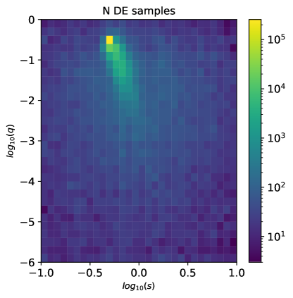
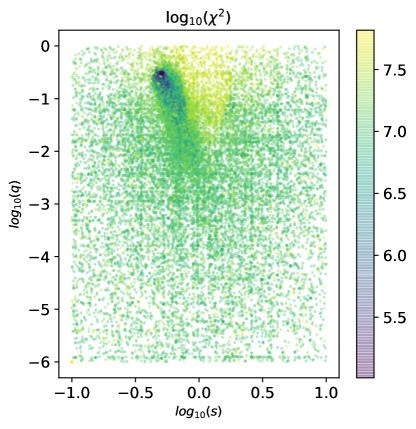
pyLIMA’s Differential Evolution (DE, Storn and Price 1997) solution-finding algorithm was used to explore parameter space and zero in on the region that best represents the data, after which we mapped the posterior distribution of each region using a Monte-Carlo Markov Chain (MCMC) algorithm (emcee; Foreman-Mackey et al. 2013). Once the parameter space minimum had been localized, the best-fitting model parameters were identified using the Levenberg-Marquardt algorithm (Levenberg, 1944; Marquardt, 1963) or the Trust Region Reflective algorithm (Coleman and Li, 1994; Branch et al., 1999).
The DE algorithm was initially given as few restrictions as possible ( to lie within 50 d of the event peak; -0.3 0.3) so that it would explore a wide parameter space and identify all possible minima for further study. The DE algorithm outputs the fit parameters for each candidate solution, which can be used to map the parameter space as shown in Figure 1. By design, the algorithm returns more solutions in regions where minima are located, so a 2D histogram of the number of solutions per element of vs. space indicates where solutions lie and further investigation is required. This exploration indicated a single but extended minimum, and consistently converged on solutions where the source-lens relative trajectory intersected the central caustic. The origin of the coordinate system was set to that of the central caustic during the modeling process, for increased stability of fit, so the impact parameter , is measured relative to this point.
Before refining the model, we reviewed the photometric uncertainties for all light curves. All photometry suffers from systematic noise at some level, and this must be quantified to avoid over-fitting the data. pyLIMA provides statistical tests of the goodness-of-fit, including a Kolmogorov-Smirnov test, an Anderson-Darling test and a Shapiro-Wilk test (Bachelet et al., 2015). If the -value returned by tests was 1%, the uncertainties on each dataset were revised, which was necessary in all cases.
Following common practise (e.g. Skowron et al. 2015), we renormalized the photometric errors, , of each dataset, , according to the expression (in magnitude units):
| (3) |
The coefficients were estimated by requiring that the reduced . If the fit could not be constrained then the coefficients were set to 0.0 and 1.0, respectively. This could occur for a variety of reasons, the most common being that the majority of measurements in a given dataset were taken primarily over the peak of the event, where the rescaling fit was heavily influenced by residuals from the model, particularly around caustic crossings. This was mitigated to some degree by iterating the model fitted with the rescaling process, to verify that the uncertainties of specific data points were not being excessively scaled. A second problem was that the photometric uncertainties for a given dataset spanned a relatively short numerical range, leading to instability in the linear regression fit of the above function, and resulting in statistically nonsensical coefficients. Lastly, for some datasets the residual scatter in the photometry was accurately represented by the uncertainties, implying that no rescaling was required. The adopted values are given in Table 3.
| Facility | ||||||||
|---|---|---|---|---|---|---|---|---|
| Chile, Dome A, fl15 | 0.0 | 1.0 | 0.0 | 1.0 | 0.0 | 1.0 | - | - |
| Chile, Dome C, fl03 | - | - | 0.0 | 1.0 | - | - | - | - |
| South Africa, Dome A, fl16 | 0.0470.03 | 1.0 | 0.0 | 1.0 | 0.0190.004 | 2.8741.597 | - | - |
| South Africa, Dome C, fl06 | - | - | 0.0 | 1.0 | 0.0 | 1.0 | - | - |
| Australia, Dome A, fl12 | 0.0 | 1.0 | 0.0 | 1.0 | 0.0 | 2.4450.831 | - | - |
| Australia, Dome B, fl11 | - | - | - | - | 0.0 | 1.0 | - | - |
| Danish, 1.54,m, DFOSC | - | - | - | - | - | - | 0.0 | 1.0 |
As there are both wide- and close-binary configurations that can produce very similar caustic structures (the well-documented close-wide degeneracy, Dominik 1999, 2009), we split the parameter space into two regions, and , which were explored separately. For this event, the close-binary solutions proved to be a significantly better fit than the wide-binary models; the parameters of the best fitting models in each case are presented in Tables 4–5. We found a significant improvement in was achieved by including microlensing parallax, which is expected for an event of this duration, and also lens binary orbital motion.
At each stage of modeling, as these effects were included, we explored finite-source, binary-lens (FSBL) models as well as USBL models. While the best-fitting of these models indicated similar parameters to the USBL models, their values were found to be somewhat higher. A close examination of the residuals showed that this is driven by a small number (5) of data points around the caustic crossing at 2458232.7, where the model is most sensitive to the limb-darkening of the source star. Two of the datapoints are in SDSS-g’ band and 3 are in SDSS-i’, which in principle might provide an independent constraint on . Regrettably, the caustic crossing occurred between the end of the night in Chile and the start of the night in Australia, and the data points were obtained from different instruments, under different conditions. This is a situation where residual systematic noise in the photometry can easily exceed the finite source signature, so proceeding with finite-source models was judged to be unsafe.
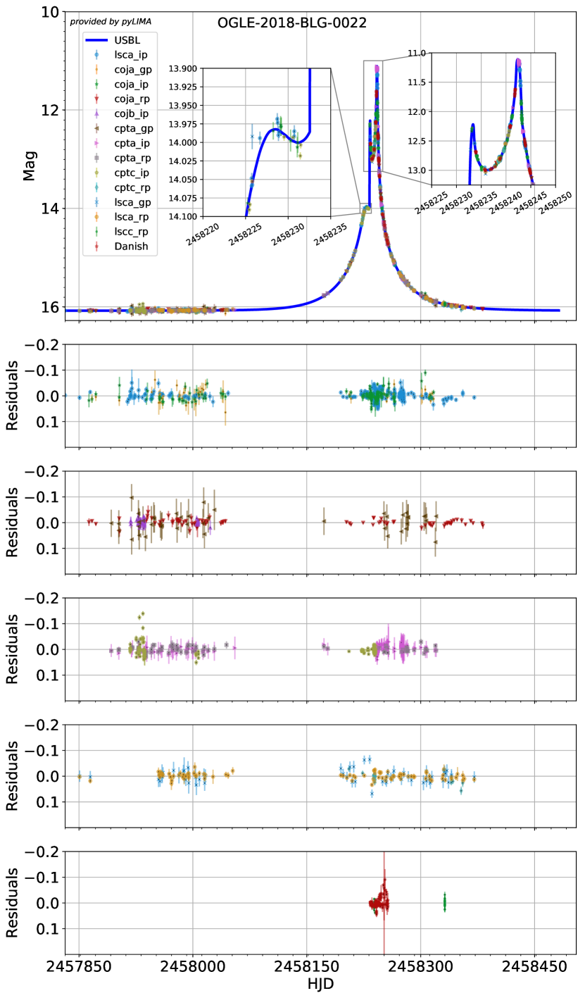
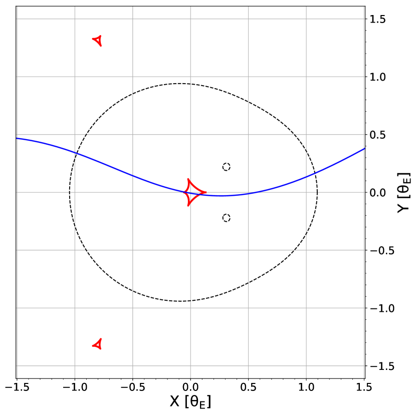
Figure 2 displays the light curve data overlaid with the best-fitting model, a uniform-source close-binary lens, and a plot of the source’s trajectory relative to the lens plane and caustic structures is shown in Figure 3. We note that there is a second degeneracy: lens-source relative trajectories with a negative value could in principle produce a very similar light curve. These solutions were allowed during our fitting process, but were always disfavored in the results. This would not strongly impact the physical characteristics of the lens inferred from the best-fit model.
 |
 |
| Parameter | Static binary | Binary+parallax | Binary+parallax | |
|---|---|---|---|---|
| +orbital motion | ||||
| USBL | USBL | USBL | FSBL | |
| [HJD] | 2458239.52808 | 2458239.98991 | 2458239.95128 | 2458240.02326 |
| 0.00317 | 0.00326 | 0.00357 | 0.00381 | |
| 0.004421 | 0.004496 | 0.004426 | 0.004526 | |
| 0.000017 | 0.000015 | 0.000019 | 0.000017 | |
| [days] | 72.767 | 70.417 | 74.905 | 75.917 |
| 0.065 | 0.069 | 0.051 | 0.071 | |
| 0.004207 | 0.004357 | 0.003967 | 0.004021 | |
| 0.000011 | 0.000013 | 0.0000089 | 0.000012 | |
| -0.29528 | -0.27221 | -0.27748 | -0.27484 | |
| 0.00017 | 0.00016 | 0.00023 | 0.00018 | |
| -0.48924 | -0.56329 | -0.58343 | -0.59851 | |
| 0.00030 | 0.00033 | 0.00024 | 0.00042 | |
| [radians] | 2.97536 | 2.95992 | 2.96006 | 2.95522 |
| 0.00032 | 0.00026 | 0.00034 | 0.00031 | |
| 0.5008 | 0.4718 | 0.4841 | ||
| 0.0021 | 0.0015 | 0.0030 | ||
| 0.0852 | 0.0664 | 0.069933 | ||
| 0.0022 | 0.0018 | 0.0031 | ||
| [/year] | 0.001158 | 0.001552 | ||
| 0.000039 | 0.000040 | |||
| [radians/year] | -0.000016 | -0.000442 | ||
| 0.000038 | 0.000043 | |||
| 16884.06 | 7239.03 | 6863.32 | 6979.39 | |
| -9645.03 | -375.71 | 116.07 | ||
| Static binary | Binary+parallax | Binary+parallax | |
|---|---|---|---|
| +orbital motion | |||
| Parameter | USBL | USBL | USBL |
| [HJD] | 2458238.66632 | 2458239.19101 | 2458240.07697 |
| 0.00373 | 0.00352 | 0.04935 | |
| -0.002834 | -0.003548 | -0.006768 | |
| 0.000015 | 0.0000099 | 0.000027 | |
| [days] | 129.3778 | 101.455 | 122.516 |
| 0.0072 | 0.091 | 0.107 | |
| 0.002042 | 0.002514 | 0.0025865 | |
| 0.000020 | 0.0000060 | 0.0000090 | |
| 0.578942 | 0.51043 | 0.44685 | |
| 0.000026 | 0.00013 | 0.00037 | |
| -0.00065 | -0.13962 | -0.33554 | |
| 0.00036 | 0.00063 | 0.00098 | |
| [radians] | -3.01041 | -2.99934 | -1.89562 |
| 0.00016 | 0.00023 | 0.00132 | |
| -0.28192 | -0.48863 | ||
| 0.00077 | 0.00315 | ||
| 0.1125 | -0.3915 | ||
| 0.0011 | 0.0018 | ||
| [/year] | -0.022095 | ||
| 0.000044 | |||
| [radians/year] | -0.007852 | ||
| 0.000013 | |||
| 36501.669 | 20519.11 | 8141.82 | |
| -15982.56 | -12377.29 |
6 Source Color Analysis
We adopted data from Chile, Dome A, camera fl15 to act as our photometric reference, since this site consistently has the best observing conditions of the whole network. After reviewing all available data, a trio of single , , images taken sequentially on 2017 July 26 between 04:05 – 04:17 UTC were selected as the reference images for these datasets because they were obtained in the best seeing, transparency and sky background conditions. These images were used as the reference images for the DIA pipeline. PSF fitting photometry was conducted on the same images, in order to determine the reference fluxes of all detected stars.
The positions of all detected stars (as determined from the World Coordinate System fit, WCS, for each image) were cross-matched against the VPHAS+ catalog (Drew et al., 2014), from which calibrated SDSS-g, -r and -i magnitudes were extracted. To mitigate the impact of differential extinction across the field of view, stars within 2 arcmin of the lensed star were selected for the purpose of measuring the photometric transformation from LCO instrumental magnitudes to the VPHAS+ system. Color-magnitude diagrams from the ROME data are presented in Figure 4.
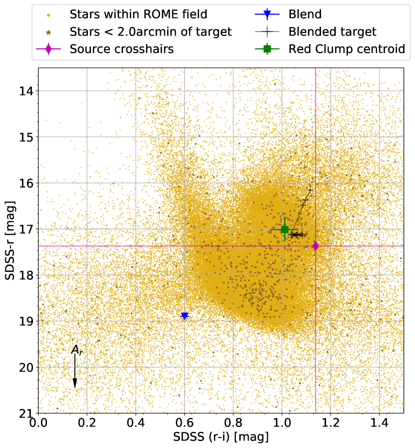
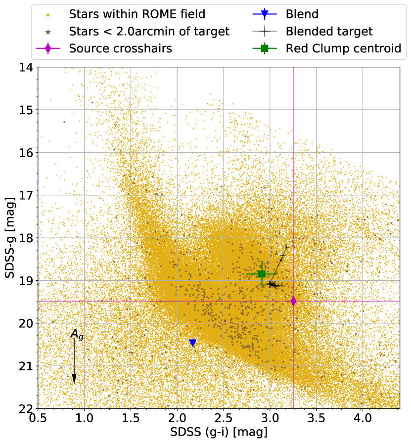
While this procedure provides an approximate photometric calibration, fields in the Galactic Bulge suffer from high extinction, which is often spatially variable across the field of view of a single ROME exposure. To account for this, it has become standard practice in microlensing to measure the offset of the Red Clump from its expected magnitude and color.
Red Clump giant stars are often used as standard candles, since their absolute luminosity is constant, being relatively insensitive to changes in metalicity and age, and they occur with high frequency across the Galactic Plane. Recently, Ruiz-Dern et al. (2018) summarized Red Clump photometric properties in a wide range of photometric systems, including their absolute magnitudes in the SDSS passbands: mag, = 0.5520.026 mag, mag.
To determine the apparent magnitude and colors of the Red Clump stars, we assume that they are located in the Galactic Bar. Nataf et al. (2013) indicated that the Galactic Bar is orientated at a viewing angle of = 40∘, meaning that the distance to the Red Clump, , is a function of Galactic longitude, :
| (4) |
where = 8.16 kpc (we note that the bar angle may be somewhat smaller, Cao et al. 2013; Wegg and Gerhard 2013, but this will cause only small changes to the results). Based on the location of OGLE-2018-BLG-0022 in Galactic coordinates = (1.82295, -2.44338)∘, the distance to the Red Clump in this field is estimated to be 7.87 kpc. We used this to estimate the apparent photometric properties (denoted by for different passbands, ) summarized in Table 6.
The Red Clump is clearly identifiable in the ROME color-magnitude diagrams (Fig. 4). Stars within 2 arcmin of the target were used to measure the centroid of the Clump in magnitude and color by applying the following selection cuts: mag, mag, mag, mag, mag. The measured centroids of the Red Clump are presented in Table 6.
taken from Ruiz-Dern et al. (2018), and the measured properties from ROME data. 1.331 0.056 mag 0.552 0.026 mag 0.262 0.032 mag 0.779 0.062 mag 1.069 0.064 mag 0.290 0.041 mag 15.810 0.056 mag 15.031 0.026 mag 14.741 0.032 mag 18.85 0.30 mag 17.01 0.25 mag 16.03 0.24 mag 1.87 0.13 mag 1.01 0.06 mag 3.037 0.056 mag 1.981 0.026 mag 1.290 0.032 mag 1.091 0.062 mag 0.722 0.041 mag
The offset of the Red Clump from its expected photometric properties was used to estimate the extinction, , and reddening, for the Red Clump along the line of sight to the target.
These quantities were then used to correct the photometric properties of the source and blend, as derived from the best-fitting light curve model, assuming that they have the same extinction and reddening as the Red Clump. The resulting data are summarized in Table 7.
| 19.484 0.007 mag | 20.462 0.027 mag | ||
| 17.369 0.002 mag | 18.895 0.013 mag | ||
| 16.231 0.001 mag | 18.294 0.013 mag | ||
| 2.115 0.007 mag | 1.567 0.030 mag | ||
| 3.253 0.007 mag | 2.168 0.030 mag | ||
| 1.138 0.002 mag | 0.601 0.018 mag | ||
| 16.447 0.056 mag | |||
| 15.388 0.026 mag | |||
| 14.941 0.032 mag | |||
| 1.059 0.007 mag | |||
| 1.506 0.007 mag | |||
| 0.447 0.002 mag |
We note that the ROME survey strategy provides a useful means to verify the source flux determined from the model. Since ROME observations are always conducted as a sequence of back-to-back (,,) exposures taken within 15 mins of each other, the magnification of the event can normally be taken to be approximately the same for all 3 images in a trio (excluding caustic crossings). These observations can be used to measure the source color and blend flux independently of the model, as follows. The total flux measured in a given passband , consists of the source flux, , multiplied by the lensing magnification, , combined with the flux from any other blended stars along the line of sight, : . Contemporaneous fluxes in multiple passbands can be combined as:
| (5) |
This allows the source color to be measured by linear regression from the slope of the fluxes in different passbands, plotted against one another. Applying this technique, we measured: = 2.1150.007 mag, = 3.2530.007 mag, = 1.1380.002 mag. These values are consistent with the colors determined from the model-predicted source fluxes in Table 7 The resulting timeseries of source color measurements are show in Fig. 4, and can be evaluated relative to the crosshairs indicating the source color measured from the light curve analysis.
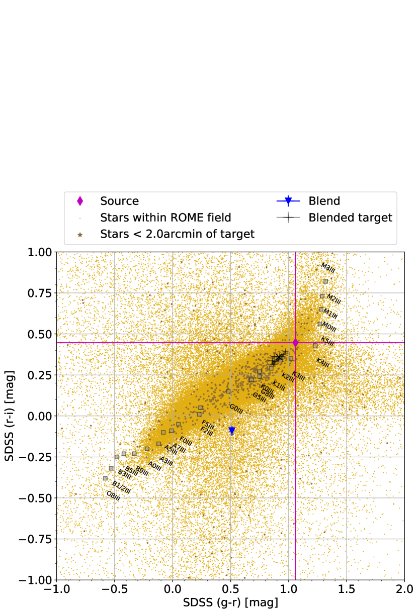
The source star’s location on the color-color diagram (Figure 5) was compared with theoretical stellar isochrones derived from the parsec model888http://stev.oapd.inaf.it/cgi-bin/cmd (Bressan et al., 2012) for solar metallicity and ages ranging from to yrs, to find the closest matching colors for each isochrone. This analysis indicated a source effective temperature of K, suggesting that the source star is a K-type star.
The angular radius, , for the source star was then calculated using the relationships between the limb-darkened and stellar colors in SDSS passbands derived from Boyajian et al. (2014). Both color indices for which coefficients were published yielded consistent estimates: as and as. We adopt an average of these two results, as.
The final required constraint is to determine the distance to the source, so that can be used to measure the Einstein radius. The best way to provide this constraint would be a measurement of the source’s parallax from the Gaia mission (Gaia Collaboration et al., 2016), although its source catalog is restricted to the brightest stars only in Bulge fields, owing to limitations of the on-board processing. The Gaia Data Release 2 catalog (Gaia Collaboration et al., 2018) reported a source (id=4062576103277425536) within 0.185 arcsec of this event, though its parallax measurement (0.132338474892901350.10027593536929187 mas) was flagged as uncertain. The catalog of distances provided by Bailer-Jones et al. (2018) gave an ill-constrained measurement of pc. It should also be borne in mind that this measurement reflects the flux of the source+blend, at baseline, and the methodology was not optimized for crowded fields.
However, the source angular radii derived from Boyajian et al. (2014) and the color indices imply that the source is a giant, and its position on the color-magnitude diagrams is consistent with a Red Clump giant in the Bulge at a distance of 7.87 kpc, as calculated earlier. Adopting this distance for the source, we infer a radius of 12.3300.666 .
Combining these quantities, with the parameters of our best-fitting model, we infer the physical properties of the lens from the following relations. The angular Einstein radius, , was extracted from the ratio of source radii in Einstein and in absolute units. This quantity relates directly to the total lens mass, , the lens distance, and the lens-source separation, .
| (6) | |||||
| (7) |
The distance to the lens was inferred from the relative parallax, , determined from our best-fit model, and the parallax to the source, :
| (8) | |||||
| (9) | |||||
| (10) |
The resulting lens properties are summarized in Table 8. The lens masses are consistent with a low-mass stellar binary composed of an M6-7 star orbiting an M3 star.
| Parameter | Units | Value |
| as | 7.2880.394 | |
| as | 1837.14599.384 | |
| 12.3270.666 | ||
| 0.4730.026 | ||
| 0.3760.020 | ||
| 0.0980.005 | ||
| Kpc | 0.9980.047 | |
| AU | 0.9670.070 | |
| mas yr-1 | 8.960.48 |
7 Assessment of the lens and blended flux
The lensing system in this case is relatively close, compared with other microlensing discoveries, and its location suggests that the binary may lie in the Galactic Disk. Given the measured masses, the simplest explanation is that the lens consists of two main sequence components. However, we noted that, with a distance modulus of 9.990.47 mag, a main sequence binary might be detectable, and we estimated its likely photometric properties as follows.
We extracted the absolute magnitudes of M-type stars from a PARSEC isochrone, assuming solar age and metallicity, and calculated the expected apparent magnitudes of the binary at the lens distance (see Table 9). These magnitudes are significantly brighter than the limiting magnitude of the ROME data (limited by the sky background, 21.969 mag [SDSS-g], 21.989 mag [SDSS-r], 22.010 mag [SDSS-i]), and suggest that the lens could be contributing to the blend flux we measured from the light curve.
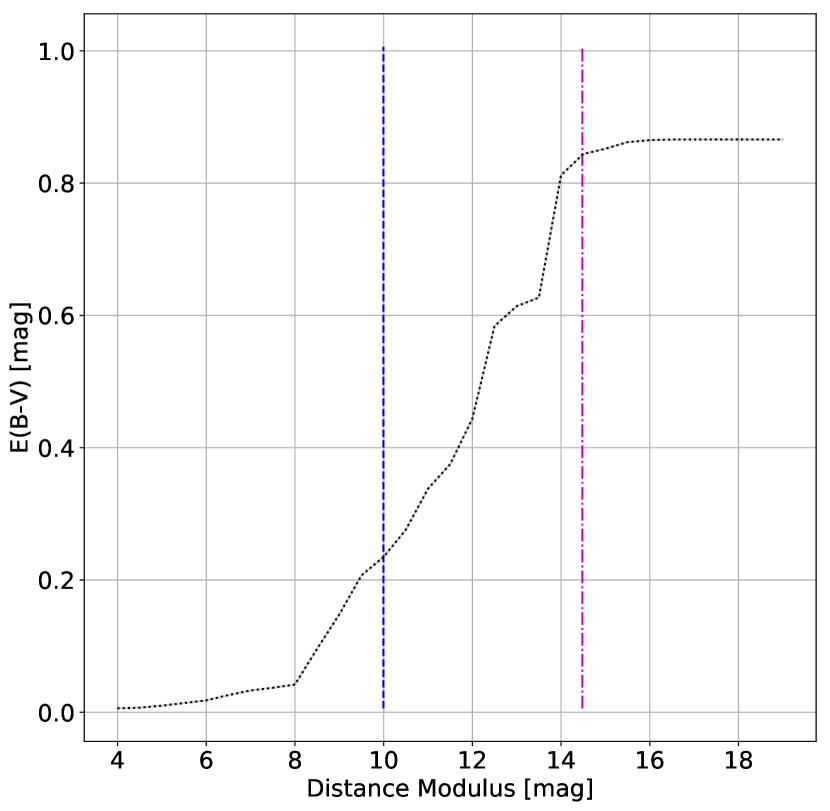
Before drawing any conclusions however, extinction and reddening must be considered. Data from the Pan-STARRS1 (Chambers et al., 2016) and 2MASS (Skrutskie et al., 2006) surveys have been combined to provided maps of the 3-dimensional reddening within the Milky Way (Green et al., 2015), which we can use to estimate this quantity along the line of sight to the source star in this event. By interpolating the data at the of this event, we estimated the colour excess to the lens star to be mag (Fig. 6). This was used to estimate the extinction in -band, , where the reddening, was estimated for the Galactic Bulge by Nataf et al. (2013) to be 2.50.2. We therefore found = 0.590.09 mag. This was used to estimate the extinction in Sloan filters by applying the transforms derived by Schlafly and Finkbeiner (2011), interpolating between the discrete values of they provided to arrive at extinction values for this field of = 0.8510.118 mag, = 0.532 0.074 mag, = 0.3820.053 mag. The extinction-corrected apparent magnitudes for the lens binary scenario are presented at the bottom of Table 9.
| Quantity | M3-dwarf | M7-dwarf | MS-binary |
|---|---|---|---|
| M3M7 | |||
| 13.175 | 21.124 | 13.174 | |
| 11.574 | 18.674 | 11.572 | |
| 11.933 | 19.149 | 11.932 | |
| 10.409 | 17.181 | 10.407 | |
| 9.475 | 14.700 | 9.466 | |
| 7.566 | 11.033 | 7.522 | |
| 7.014 | 10.458 | 6.969 | |
| 6.779 | 10.178 | 6.733 | |
| 1.601 | 2.450 | 1.602 | |
| 1.524 | 1.968 | 1.525 | |
| 0.934 | 2.481 | 0.941 | |
| 0.552 | 0.575 | 0.553 | |
| 0.235 | 0.280 | 0.237 | |
| 0.787 | 0.855 | 0.790 | |
| 23.169 | 31.118 | 23.168 | |
| 21.568 | 28.668 | 21.566 | |
| 21.927 | 29.143 | 21.926 | |
| 20.403 | 27.175 | 20.401 | |
| 19.469 | 24.694 | 19.460 | |
| 17.560 | 21.027 | 17.516 | |
| 17.008 | 20.452 | 16.963 | |
| 16.773 | 20.172 | 16.727 | |
| 22.155 | 29.255 | 22.153 | |
| 1.836 | 2.685 | 1.837 | |
| 22.778 | 29.994 | 22.777 | |
| 20.935 | 27.707 | 20.933 | |
| 19.851 | 25.076 | 19.842 | |
| 1.843 | 2.287 | 1.844 | |
| 1.084 | 2.631 | 1.091 |
The measured blend photometry in Table 7 indicates one or more objects that are significantly brighter than the photometry predicted for a main sequence M3+M7 binary, implying that the light originates from a separate object(s) – a common situation in the crowded star fields of the Galactic Bulge. Nevertheless, we note that the lens should be easily detectable in 2–4 m-class telescopes, particularly in the NIR.
8 Conclusions
The microlensing event OGLE-2018-BLG-0022 revealed the presence of an M3+M7 binary star, previously undetected owing to its intrinsically low luminosity. That said, the binary in this event is unusually close to the Earth for a microlens – 1 kpc away – and the object shows a correspondingly high relative proper motion of 8.96 mas yr-1. This makes it a good candidate for high spatial resolution AO imaging in the relatively near future which, as discussed by Henderson et al. (2014), could provide an independent verification of the lens mass determination. While the proximity of the lens, resulting in a large (1.84 mas) angular Einstein radius, would have been resolvable to interferometry, as demonstrated by Dong et al. (2018), the source star in this case was too faint for current instruments. The discovery highlight’s microlensing’s capability to map populations beyond the solar neighborhood that would otherwise be hidden by their intrinsically faint luminosities.
9 Acknowledgements
RAS and EB gratefully acknowledge support from NASA grant NNX15AC97G. YT and JW acknowledge the support of DFG priority program SPP 1992 “Exploring the Diversity of Extrasolar Planets” (WA 1047/11-1). KH acknowledges support from STFC grant ST/R000824/1. This research has made use of NASA’s Astrophysics Data System, and the NASA Exoplanet Archive. The work was partly based on data products from observations made with ESO Telescopes at the La Silla Paranal Observatory under programme ID 177.D-3023, as part of the VST Photometric Halpha Survey of the Southern Galactic Plane and Bulge (VPHAS+, www.vphas.eu). This work also made use of data from the European Space Agency (ESA) mission Gaia (https://www.cosmos.esa.int/gaia), processed by the Gaia Data Processing and Analysis Consortium (DPAC, https://www.cosmos.esa.int/web/gaia/dpac/consortium). Funding for the DPAC has been provided by national institutions, in particular the institutions participating in the Gaia Multilateral Agreement. CITEUC is funded by National Funds through FCT - Foundation for Science and Technology (project: UID/Multi/00611/2013) and FEDER - European Regional Development Fund through COMPETE 2020 – Operational Programme Competitiveness and Internationalization (project: POCI-01-0145-FEDER-006922). The work by SS and SR was supported by a grant (95843339) from the Iran National Science Foundation (INSF). DMB acknowledges the support of the NYU Abu Dhabi Research Enhancement Fund under grant RE124. This research uses data obtained through the Telescope Access Program (TAP), which has been funded by the National Astronomical Observatories of China, the Chinese Academy of Sciences, and the Special Fund for Astronomy from the Ministry of Finance. This work was partly supported by the National Science Foundation of China (Grant No. 11333003, 11390372 and 11761131004 to SM).
References
- Albrow et al. [1999] M. D. Albrow, J.-P. Beaulieu, J. A. R. Caldwell, D. L. DePoy, M. Dominik, B. S. Gaudi, A. Gould, J. Greenhill, K. Hill, S. Kane, R. Martin, J. Menzies, R. M. Naber, R. W. Pogge, K. R. Pollard, P. D. Sackett, K. C. Sahu, P. Vermaak, R. Watson, A. Williams, and PLANET Collaboration. A Complete Set of Solutions for Caustic Crossing Binary Microlensing Events. ApJ, 522:1022–1036, September 1999. 10.1086/307699.
- Bachelet et al. [2015] E. Bachelet, D. M. Bramich, C. Han, J. Greenhill, R. A. Street, A. Gould, G. D’Ago, K. AlSubai, M. Dominik, R. Figuera Jaimes, K. Horne, M. Hundertmark, N. Kains, C. Snodgrass, I. A. Steele, Y. Tsapras, RoboNet Collaboration, M. D. Albrow, V. Batista, J.-P. Beaulieu, D. P. Bennett, S. Brillant, J. A. R. Caldwell, A. Cassan, A. Cole, C. Coutures, S. Dieters, D. Dominis Prester, J. Donatowicz, P. Fouqué, K. Hill, J.-B. Marquette, J. Menzies, C. Pere, C. Ranc, J. Wambsganss, D. Warren, PLANET Collaboration, L. A. de Almeida, J.-Y. Choi, D. L. DePoy, S. Dong, L.-W. Hung, K.-H. Hwang, F. Jablonski, Y. K. Jung, S. Kaspi, N. Klein, C.-U. Lee, D. Maoz, J. A. Muñoz, D. Nataf, H. Park, R. W. Pogge, D. Polishook, I.-G. Shin, A. Shporer, J. C. Yee, FUN Collaboration, F. Abe, A. Bhattacharya, I. A. Bond, C. S. Botzler, M. Freeman, A. Fukui, Y. Itow, N. Koshimoto, C. H. Ling, K. Masuda, Y. Matsubara, Y. Muraki, K. Ohnishi, L. C. Philpott, N. Rattenbury, T. Saito, D. J. Sullivan, T. Sumi, D. Suzuki, P. J. Tristram, A. Yonehara, MOA Collaboration, V. Bozza, S. Calchi Novati, S. Ciceri, P. Galianni, S.-H. Gu, K. Harpsøe, T. C. Hinse, U. G. Jørgensen, D. Juncher, H. Korhonen, L. Mancini, C. Melchiorre, A. Popovas, A. Postiglione, M. Rabus, S. Rahvar, R. W. Schmidt, G. Scarpetta, J. Skottfelt, J. Southworth, A. Stabile, J. Surdej, X.-B. Wang, O. Wertz, and MiNDSTEp Collaboration. Red Noise Versus Planetary Interpretations in the Microlensing Event Ogle-2013-BLG-446. ApJ, 812:136, October 2015. 10.1088/0004-637X/812/2/136.
- Bachelet et al. [2017] E. Bachelet, M. Norbury, V. Bozza, and R. Street. pyLIMA: An Open-source Package for Microlensing Modeling. I. Presentation of the Software and Analysis of Single-lens Models. AJ, 154:203, November 2017. 10.3847/1538-3881/aa911c.
- Bailer-Jones et al. [2018] C. A. L. Bailer-Jones, J. Rybizki, M. Fouesneau, G. Mantelet, and R. Andrae. Estimating Distance from Parallaxes. IV. Distances to 1.33 Billion Stars in Gaia Data Release 2. AJ, 156:58, August 2018. 10.3847/1538-3881/aacb21.
- Bond et al. [2001] I. A. Bond, F. Abe, R. J. Dodd, J. B. Hearnshaw, M. Honda, J. Jugaku, P. M. Kilmartin, A. Marles, K. Masuda, Y. Matsubara, Y. Muraki, T. Nakamura, G. Nankivell, S. Noda, C. Noguchi, K. Ohnishi, N. J. Rattenbury, M. Reid, T. Saito, H. Sato, M. Sekiguchi, J. Skuljan, D. J. Sullivan, T. Sumi, M. Takeuti, Y. Watase, S. Wilkinson, R. Yamada, T. Yanagisawa, and P. C. M. Yock. Real-time difference imaging analysis of MOA Galactic bulge observations during 2000. MNRAS, 327:868–880, November 2001. 10.1046/j.1365-8711.2001.04776.x.
- Boyajian et al. [2014] T. S. Boyajian, G. van Belle, and K. von Braun. Stellar Diameters and Temperatures. IV. Predicting Stellar Angular Diameters. AJ, 147:47, March 2014. 10.1088/0004-6256/147/3/47.
- Bozza [2010] V. Bozza. Microlensing with an advanced contour integration algorithm: Green’s theorem to third order, error control, optimal sampling and limb darkening. MNRAS, 408:2188–2200, November 2010. 10.1111/j.1365-2966.2010.17265.x.
- Bozza et al. [2018] V. Bozza, E. Bachelet, F. Bartolić, T. M. Heintz, A. R. Hoag, and M. Hundertmark. VBBINARYLENSING: a public package for microlensing light-curve computation. MNRAS, 479:5157–5167, October 2018. 10.1093/mnras/sty1791.
- Bramich [2008] D. M. Bramich. A new algorithm for difference image analysis. MNRAS, 386:L77–L81, May 2008. 10.1111/j.1745-3933.2008.00464.x.
- Bramich [2018] D. M. Bramich. Predicted microlensing events from analysis of Gaia Data Release 2. A&A, 618:A44, October 2018. 10.1051/0004-6361/201833505.
- Bramich et al. [2013] D. M. Bramich, K. Horne, M. D. Albrow, Y. Tsapras, C. Snodgrass, R. A. Street, M. Hundertmark, N. Kains, A. Arellano Ferro, J. R. Figuera, and S. Giridhar. Difference image analysis: extension to a spatially varying photometric scale factor and other considerations. MNRAS, 428:2275–2289, January 2013. 10.1093/mnras/sts184.
- Branch et al. [1999] M.A. Branch, F.T. Coleman, and Y. Li. A subspace, interior, and conjugate gradient method for large-scale bound-constrained minimization problems. SIAM Journal on Scientific Computing, 21, 12 1999. 10.1137/S1064827595289108.
- Bressan et al. [2012] A. Bressan, P. Marigo, L. Girardi, B. Salasnich, C. Dal Cero, S. Rubele, and A. Nanni. PARSEC: stellar tracks and isochrones with the PAdova and TRieste Stellar Evolution Code. MNRAS, 427:127–145, November 2012. 10.1111/j.1365-2966.2012.21948.x.
- Brown et al. [2013] T. M. Brown, N. Baliber, F. B. Bianco, M. Bowman, B. Burleson, P. Conway, M. Crellin, É. Depagne, J. De Vera, B. Dilday, D. Dragomir, M. Dubberley, J. D. Eastman, M. Elphick, M. Falarski, S. Foale, M. Ford, B. J. Fulton, J. Garza, E. L. Gomez, M. Graham, R. Greene, B. Haldeman, E. Hawkins, B. Haworth, R. Haynes, M. Hidas, A. E. Hjelstrom, D. A. Howell, J. Hygelund, T. A. Lister, R. Lobdill, J. Martinez, D. S. Mullins, M. Norbury, J. Parrent, R. Paulson, D. L. Petry, A. Pickles, V. Posner, W. E. Rosing, R. Ross, D. J. Sand, E. S. Saunders, J. Shobbrook, A. Shporer, R. A. Street, D. Thomas, Y. Tsapras, J. R. Tufts, S. Valenti, K. Vander Horst, Z. Walker, G. White, and M. Willis. Las Cumbres Observatory Global Telescope Network. PASP, 125:1031, September 2013. 10.1086/673168.
- Cao et al. [2013] L. Cao, S. Mao, D. Nataf, N. J. Rattenbury, and A. Gould. A new photometric model of the Galactic bar using red clump giants. MNRAS, 434:595–605, September 2013. 10.1093/mnras/stt1045.
- Chambers et al. [2016] K. C. Chambers, E. A. Magnier, N. Metcalfe, H. A. Flewelling, M. E. Huber, C. Z. Waters, L. Denneau, P. W. Draper, D. Farrow, D. P. Finkbeiner, C. Holmberg, J. Koppenhoefer, P. A. Price, R. P. Saglia, E. F. Schlafly, S. J. Smartt, W. Sweeney, R. J. Wainscoat, W. S. Burgett, T. Grav, J. N. Heasley, K. W. Hodapp, R. Jedicke, N. Kaiser, R.-P. Kudritzki, G. A. Luppino, R. H. Lupton, D. G. Monet, J. S. Morgan, P. M. Onaka, C. W. Stubbs, J. L. Tonry, E. Banados, E. F. Bell, R. Bender, E. J. Bernard, M. T. Botticella, S. Casertano, S. Chastel, W.-P. Chen, X. Chen, S. Cole, N. Deacon, C. Frenk, A. Fitzsimmons, S. Gezari, C. Goessl, T. Goggia, B. Goldman, E. K. Grebel, N. C. Hambly, G. Hasinger, A. F. Heavens, T. M. Heckman, R. Henderson, T. Henning, M. Holman, U. Hopp, W.-H. Ip, S. Isani, C. D. Keyes, A. Koekemoer, R. Kotak, K. S. Long, J. R Lucey, M. Liu, N. F. Martin, B. McLean, E. Morganson, D. N. A. Murphy, M. A. Nieto-Santisteban, P. Norberg, J. A. Peacock, E. A. Pier, M. Postman, N. Primak, C. Rae, A. Rest, A. Riess, A. Riffeser, H. W. Rix, S. Roser, E. Schilbach, A. S. B. Schultz, D. Scolnic, A. Szalay, S. Seitz, B. Shiao, E. Small, K. W. Smith, D. Soderblom, A. N. Taylor, A. R. Thakar, J. Thiel, D. Thilker, Y. Urata, J. Valenti, F. Walter, S. P. Watters, S. Werner, R. White, W. M. Wood-Vasey, and R. Wyse. The Pan-STARRS1 Surveys. ArXiv e-prints, December 2016.
- Claret and Bloemen [2011] A. Claret and S. Bloemen. Gravity and limb-darkening coefficients for the Kepler, CoRoT, Spitzer, uvby, UBVRIJHK, and Sloan photometric systems. A&A, 529:A75, May 2011. 10.1051/0004-6361/201116451.
- Coleman and Li [1994] F.T. Coleman and Y. Li. On the convergence of reflective newton methods for large-scale nonlinear minimization subject to bounds. Math. Program., 67:189–224, 10 1994. 10.1007/BF01582221.
- Dominik [1999] M. Dominik. The binary gravitational lens and its extreme cases. A&A, 349:108–125, September 1999.
- Dominik [2009] M. Dominik. Parameter degeneracies and (un)predictability of gravitational microlensing events. MNRAS, 393:816–821, March 2009. 10.1111/j.1365-2966.2008.14276.x.
- Dominik et al. [2007] M. Dominik, N. J. Rattenbury, A. Allan, S. Mao, D. M. Bramich, M. J. Burgdorf, E. Kerins, Y. Tsapras, and Ł. Wyrzykowski. An anomaly detector with immediate feedback to hunt for planets of Earth mass and below by microlensing. MNRAS, 380:792–804, September 2007. 10.1111/j.1365-2966.2007.12124.x.
- Dominik et al. [2008b] M. Dominik, K. Horne, A. Allan, N. J. Rattenbury, Y. Tsapras, C. Snodgrass, M. F. Bode, M. J. Burgdorf, S. N. Fraser, E. Kerins, C. J. Mottram, I. A. Steele, R. A. Street, P. J. Wheatley, and Ł. Wyrzykowski. ARTEMiS (Automated Robotic Terrestrial Exoplanet Microlensing Search): A possible expert-system based cooperative effort to hunt for planets of Earth mass and below. Astronomische Nachrichten, 329:248, March 2008b. 10.1002/asna.200710928.
- Dominik et al. [2008a] M. Dominik, K. Horne, A. Allan, N. J. Rattenbury, Y. Tsapras, C. Snodgrass, M. F. Bode, M. J. Burgdorf, S. N. Fraser, E. Kerins, C. J. Mottram, I. A. Steele, R. A. Street, P. J. Wheatley, and Ł. Wyrzykowski. ARTEMiS (Automated Robotic Terrestrial Exoplanet Microlensing Search): A possible expert-system based cooperative effort to hunt for planets of Earth mass and below. Astronomische Nachrichten, 329:248, March 2008a. 10.1002/asna.200710928.
- Dominik et al. [2010] M. Dominik, U. G. Jørgensen, N. J. Rattenbury, M. Mathiasen, T. C. Hinse, S. Calchi Novati, K. Harpsøe, V. Bozza, T. Anguita, M. J. Burgdorf, K. Horne, M. Hundertmark, E. Kerins, P. Kjærgaard, C. Liebig, L. Mancini, G. Masi, S. Rahvar, D. Ricci, G. Scarpetta, C. Snodgrass, J. Southworth, R. A. Street, J. Surdej, C. C. Thöne, Y. Tsapras, J. Wambsganss, and M. Zub. Realisation of a fully-deterministic microlensing observing strategy for inferring planet populations. Astronomische Nachrichten, 331:671, July 2010. 10.1002/asna.201011400.
- Dong et al. [2007] S. Dong, A. Udalski, A. Gould, W. T. Reach, G. W. Christie, A. F. Boden, D. P. Bennett, G. Fazio, K. Griest, M. K. Szymański, M. Kubiak, I. Soszyński, G. Pietrzyński, O. Szewczyk, Ł. Wyrzykowski, K. Ulaczyk, T. Wieckowski, B. Paczyński, D. L. DePoy, R. W. Pogge, G. W. Preston, I. B. Thompson, and B. M. Patten. First Space-Based Microlens Parallax Measurement: Spitzer Observations of OGLE-2005-SMC-001. ApJ, 664:862–878, August 2007. 10.1086/518536.
- Dong et al. [2018] Subo Dong, A. Mérand, F. Delplancke-Ströbele, Andrew Gould, Ping Chen, R. Post, C. S. Kochanek, K. Z. Stanek, G. W. Christie, Robert Mutel, T. Natusch, T. W. S. Holoien, J. L. Prieto, B. J. Shappee, and Todd A. Thompson. First Resolution of Microlensed Images. arXiv e-prints, art. arXiv:1809.08243, September 2018.
- Drew et al. [2014] J. E. Drew, E. Gonzalez-Solares, R. Greimel, M. J. Irwin, A. Küpcü Yoldas, J. Lewis, G. Barentsen, J. Eislöffel, H. J. Farnhill, W. E. Martin, J. R. Walsh, N. A. Walton, M. Mohr-Smith, R. Raddi, S. E. Sale, N. J. Wright, P. Groot, M. J. Barlow, R. L. M. Corradi, J. J. Drake, J. Fabregat, D. J. Frew, B. T. Gänsicke, C. Knigge, A. Mampaso, R. A. H. Morris, T. Naylor, Q. A. Parker, S. Phillipps, C. Ruhland, D. Steeghs, Y. C. Unruh, J. S. Vink, R. Wesson, and A. A. Zijlstra. The VST Photometric H Survey of the Southern Galactic Plane and Bulge (VPHAS+). MNRAS, 440:2036–2058, May 2014. 10.1093/mnras/stu394.
- Evans et al. [2016] D. F. Evans, J. Southworth, P. F. L. Maxted, J. Skottfelt, M. Hundertmark, U. G. Jørgensen, M. Dominik, K. A. Alsubai, M. I. Andersen, V. Bozza, D. M. Bramich, M. J. Burgdorf, S. Ciceri, G. D’Ago, R. Figuera Jaimes, S.-H. Gu, T. Haugbølle, T. C. Hinse, D. Juncher, N. Kains, E. Kerins, H. Korhonen, M. Kuffmeier, L. Mancini, N. Peixinho, A. Popovas, M. Rabus, S. Rahvar, R. W. Schmidt, C. Snodgrass, D. Starkey, J. Surdej, R. Tronsgaard, C. von Essen, Y.-B. Wang, and O. Wertz. High-resolution Imaging of Transiting Extrasolar Planetary systems (HITEP). I. Lucky imaging observations of 101 systems in the southern hemisphere. A&A, 589:A58, May 2016. https://doi.org/10.1051/0004-6361/201527970.
- Foreman-Mackey et al. [2013] D. Foreman-Mackey, D. W. Hogg, D. Lang, and J. Goodman. emcee: The MCMC Hammer. PASP, 125:306, March 2013. 10.1086/670067.
- Gaia Collaboration et al. [2016] Gaia Collaboration, T. Prusti, J. H. J. de Bruijne, A. G. A. Brown, A. Vallenari, C. Babusiaux, C. A. L. Bailer-Jones, U. Bastian, M. Biermann, D. W. Evans, and et al. The Gaia mission. A&A, 595:A1, November 2016. 10.1051/0004-6361/201629272.
- Gaia Collaboration et al. [2018] Gaia Collaboration, A. G. A. Brown, A. Vallenari, T. Prusti, J. H. J. de Bruijne, C. Babusiaux, and C. A. L. Bailer-Jones. Gaia Data Release 2. Summary of the contents and survey properties. ArXiv e-prints, April 2018.
- Green et al. [2015] G. M. Green, E. F. Schlafly, D. P. Finkbeiner, H.-W. Rix, N. Martin, W. Burgett, P. W. Draper, H. Flewelling, K. Hodapp, N. Kaiser, R. P. Kudritzki, E. Magnier, N. Metcalfe, P. Price, J. Tonry, and R. Wainscoat. A Three-dimensional Map of Milky Way Dust. ApJ, 810:25, September 2015. 10.1088/0004-637X/810/1/25.
- Henderson et al. [2014] C. B. Henderson, H. Park, T. Sumi, A. Udalski, A. Gould, Y. Tsapras, C. Han, B. S. Gaudi, V. Bozza, F. Abe, D. P. Bennett, I. A. Bond, C. S. Botzler, M. Freeman, A. Fukui, D. Fukunaga, Y. Itow, N. Koshimoto, C. H. Ling, K. Masuda, Y. Matsubara, Y. Muraki, S. Namba, K. Ohnishi, N. J. Rattenbury, To Saito, D. J. Sullivan, D. Suzuki, W. L. Sweatman, P. J. Tristram, N. Tsurumi, K. Wada, N. Yamai, P. C. M. Yock, A. Yonehara, MOA Collaboration, M. K. Szymański, M. Kubiak, G. Pietrzyński, I. Soszyński, J. Skowron, S. Kozłowski, R. Poleski, K. Ulaczyk, Ł. Wyrzykowski, P. Pietrukowicz, OGLE Collaboration, L. A. Almeida, M. Bos, J. Y. Choi, G. W. Christie, D. L. Depoy, S. Dong, M. Friedmann, K. H. Hwang, F. Jablonski, Y. K. Jung, S. Kaspi, C. U. Lee, D. Maoz, J. McCormick, D. Moorhouse, T. Natusch, H. Ngan, R. W. Pogge, I. G. Shin, Y. Shvartzvald, T. G. Tan, G. Thornley, J. C. Yee, FUN Collaboration, A. Allan, D. M. Bramich, P. Browne, M. Dominik, K. Horne, M. Hundertmark, R. Figuera Jaimes, N. Kains, C. Snodgrass, I. A. Steele, R. A. Street, and RoboNet Collaboration. Candidate Gravitational Microlensing Events for Future Direct Lens Imaging. ApJ, 794:71, October 2014. 10.1088/0004-637X/794/1/71.
- Hundertmark et al. [2018] M. Hundertmark, R. A. Street, Y. Tsapras, E. Bachelet, M. Dominik, K. Horne, V. Bozza, D. M. Bramich, A. Cassan, G. D’Ago, R. Figuera Jaimes, N. Kains, C. Ranc, R. W. Schmidt, C. Snodgrass, J. Wambsganss, I. A. Steele, S. Mao, K. Ment, J. Menzies, Z. Li, S. Cross, D. Maoz, and Y. Shvartzvald. RoboTAP: Target priorities for robotic microlensing observations. A&A, 609:A55, January 2018. 10.1051/0004-6361/201730692.
- Levenberg [1944] K. Levenberg. A Method for the Solution of Certain Non-Linear Problems in Least Squares. Quarterly of Applied Mathematics, 2:164, 1944.
- Marquardt [1963] D. Marquardt. An Algorithm for Least-Squares Estimation of Nonlinear Parameters. SIAM Journal on Applied Mathematics, 11:431, 1963. 10.1137/0111030.
- Minniti et al. [2010] D. Minniti, P. W. Lucas, J. P. Emerson, R. K. Saito, M. Hempel, P. Pietrukowicz, A. V. Ahumada, M. V. Alonso, J. Alonso-Garcia, J. I. Arias, R. M. Bandyopadhyay, R. H. Barbá, B. Barbuy, L. R. Bedin, E. Bica, J. Borissova, L. Bronfman, G. Carraro, M. Catelan, J. J. Clariá, N. Cross, R. de Grijs, I. Dékány, J. E. Drew, C. Fariña, C. Feinstein, E. Fernández Lajús, R. C. Gamen, D. Geisler, W. Gieren, B. Goldman, O. A. Gonzalez, G. Gunthardt, S. Gurovich, N. C. Hambly, M. J. Irwin, V. D. Ivanov, A. Jordán, E. Kerins, K. Kinemuchi, R. Kurtev, M. López-Corredoira, T. Maccarone, N. Masetti, D. Merlo, M. Messineo, I. F. Mirabel, L. Monaco, L. Morelli, N. Padilla, T. Palma, M. C. Parisi, G. Pignata, M. Rejkuba, A. Roman-Lopes, S. E. Sale, M. R. Schreiber, A. C. Schröder, M. Smith, Jr. , L. Sodré, M. Soto, M. Tamura, C. Tappert, M. A. Thompson, I. Toledo, M. Zoccali, and G. Pietrzynski. VISTA Variables in the Via Lactea (VVV): The public ESO near-IR variability survey of the Milky Way. New A, 15:433–443, July 2010. 10.1016/j.newast.2009.12.002.
- Nataf et al. [2013] D. M. Nataf, A. Gould, P. Fouqué, O. A. Gonzalez, J. A. Johnson, J. Skowron, A. Udalski, M. K. Szymański, M. Kubiak, G. Pietrzyński, I. Soszyński, K. Ulaczyk, Ł. Wyrzykowski, and R. Poleski. Reddening and Extinction toward the Galactic Bulge from OGLE-III: The Inner Milky Way’s RV ~ 2.5 Extinction Curve. ApJ, 769:88, June 2013. 10.1088/0004-637X/769/2/88.
- Park et al. [2012] B.-G. Park, S.-L. Kim, J. W. Lee, B.-C. Lee, C.-U. Lee, C. Han, M. Kim, D.-S. Moon, H.-K. Moon, S.-C. Rey, E.-C. Sung, and H. Sung. Korea Microlensing Telescope Network: science cases. In Ground-based and Airborne Telescopes IV, volume 8444 of Proc. SPIE, page 844447, September 2012. 10.1117/12.925826.
- Pickles [1998] A. J. Pickles. A Stellar Spectral Flux Library: 1150-25000 Å. PASP, 110:863–878, July 1998. 10.1086/316197.
- Refsdal [1964] S. Refsdal. The gravitational lens effect. MNRAS, 128:295, 1964. 10.1093/mnras/128.4.295.
- Ruiz-Dern et al. [2018] L. Ruiz-Dern, C. Babusiaux, F. Arenou, C. Turon, and R. Lallement. Empirical photometric calibration of the Gaia red clump: Colours, effective temperature, and absolute magnitude. A&A, 609:A116, January 2018. 10.1051/0004-6361/201731572.
- Sako et al. [2008] T. Sako, T. Sekiguchi, M. Sasaki, K. Okajima, F. Abe, I. A. Bond, J. B. Hearnshaw, Y. Itow, K. Kamiya, P. M. Kilmartin, K. Masuda, Y. Matsubara, Y. Muraki, N. J. Rattenbury, D. J. Sullivan, T. Sumi, P. Tristram, T. Yanagisawa, and P. C. M. Yock. MOA-cam3: a wide-field mosaic CCD camera for a gravitational microlensing survey in New Zealand. Experimental Astronomy, 22:51–66, October 2008. 10.1007/s10686-007-9082-5.
- Saunders et al. [2014] E.S. Saunders, S. Lampoudi, T.A. Lister, M. Norbury, and Z. Walker. Novel scheduling approaches in the era of multi-telescope networks, 2014. URL https://doi.org/10.1117/12.2056642.
- Schlafly and Finkbeiner [2011] E. F. Schlafly and D. P. Finkbeiner. Measuring Reddening with Sloan Digital Sky Survey Stellar Spectra and Recalibrating SFD. ApJ, 737:103, August 2011. 10.1088/0004-637X/737/2/103.
- Shvartzvald et al. [2016] Y. Shvartzvald, Z. Li, A. Udalski, A. Gould, T. Sumi, R. A. Street, S. Calchi Novati, M. Hundertmark, V. Bozza, C. Beichman, G. Bryden, S. Carey, J. Drummond, M. Fausnaugh, B. S. Gaudi, C. B. Henderson, T. G. Tan, B. Wibking, R. W. Pogge, J. C. Yee, W. Zhu, (Spitzer Team, Y. Tsapras, E. Bachelet, M. Dominik, D. M. Bramich, A. Cassan, R. Figuera Jaimes, K. Horne, C. Ranc, R. Schmidt, C. Snodgrass, J. Wambsganss, I. A. Steele, J. Menzies, S. Mao, (RoboNet, R. Poleski, M. Pawlak, M. K. Szymański, J. Skowron, P. Mróz, S. Kozłowski, Ł. Wyrzykowski, P. Pietrukowicz, I. Soszyński, K. Ulaczyk, (OGLE Group, F. Abe, Y. Asakura, R. K. Barry, D. P. Bennett, A. Bhattacharya, I. A. Bond, M. Freeman, Y. Hirao, Y. Itow, N. Koshimoto, M. C. A. Li, C. H. Ling, K. Masuda, A. Fukui, Y. Matsubara, Y. Muraki, M. Nagakane, T. Nishioka, K. Ohnishi, H. Oyokawa, N. J. Rattenbury, T. Saito, A. Sharan, D. J. Sullivan, D. Suzuki, P. J. Tristram, A. Yonehara, (MOA Group, U. G. Jørgensen, M. J. Burgdorf, S. Ciceri, G. D’Ago, D. F. Evans, T. C. Hinse, N. Kains, E. Kerins, H. Korhonen, L. Mancini, A. Popovas, M. Rabus, S. Rahvar, G. Scarpetta, J. Skottfelt, J. Southworth, N. Peixinho, P. Verma, (MiNDSTEp, B. Sbarufatti, J. A. Kennea, N. Gehrels, and (Swift. The First Simultaneous Microlensing Observations by Two Space Telescopes: Spitzer and Swift Reveal a Brown Dwarf in Event OGLE-2015-BLG-1319. ApJ, 831:183, November 2016. 10.3847/0004-637X/831/2/183.
- Shvartzvald et al. [2017] Y. Shvartzvald, G. Bryden, A. Gould, C. B. Henderson, S. B. Howell, and C. Beichman. UKIRT Microlensing Surveys as a Pathfinder for WFIRST: The Detection of Five Highly Extinguished Low-b Events. AJ, 153:61, February 2017. 10.3847/1538-3881/153/2/61.
- Skottfelt et al. [2015] J. Skottfelt, D. M. Bramich, M. Hundertmark, U. G. Jørgensen, N. Michaelsen, P. Kjærgaard, J. Southworth, A. N. Sørensen, M. F. Andersen, M. I. Andersen, J. Christensen-Dalsgaard, S. Frandsen, F. Grundahl, K. B. W. Harpsøe, H. Kjeldsen, and P. L. Pallé. The two-colour EMCCD instrument for the Danish 1.54 m telescope and SONG. A&A, 574:A54, February 2015. https://doi.org/10.1051/0004-6361/201425260.
- Skowron et al. [2015] J. Skowron, I. G. Shin, A. Udalski, C. Han, T. Sumi, Y. Shvartzvald, A. Gould, D. Dominis Prester, R. A. Street, U. G. Jørgensen, D. P. Bennett, V. Bozza, M. K. Szymański, M. Kubiak, G. Pietrzyński, I. Soszyński, R. Poleski, S. Kozłowski, P. Pietrukowicz, K. Ulaczyk, Ł. Wyrzykowski, OGLE Collaboration, F. Abe, A. Bhattacharya, I. A. Bond, C. S. Botzler, M. Freeman, A. Fukui, D. Fukunaga, Y. Itow, C. H. Ling, N. Koshimoto, K. Masuda, Y. Matsubara, Y. Muraki, S. Namba, K. Ohnishi, L. C. Philpott, N. Rattenbury, T. Saito, D. J. Sullivan, D. Suzuki, P. J. Tristram, P. C. M. Yock, MOA Collaboration, D. Maoz, S. Kaspi, M. Friedmann, Wise Group, L. A. Almeida, V. Batista, G. Christie, J. Y. Choi, D. L. DePoy, B. S. Gaudi, C. Henderson, K. H. Hwang, F. Jablonski, Y. K. Jung, C. U. Lee, J. McCormick, T. Natusch, H. Ngan, H. Park, R. W. Pogge, J. C. Yee, FUN Collaboration, M. D. Albrow, E. Bachelet, J. P. Beaulieu, S. Brillant, J. A. R. Caldwell, A. Cassan, A. Cole, E. Corrales, Ch. Coutures, S. Dieters, J. Donatowicz, P. Fouqué, J. Greenhill, N. Kains, S. R. Kane, D. Kubas, J. B. Marquette, R. Martin, J. Menzies, K. R. Pollard, C. Ranc, K. C. Sahu, J. Wambsganss, A. Williams, D. Wouters, PLANET Collaboration, Y. Tsapras, D. M. Bramich, K. Horne, M. Hundertmark, C. Snodgrass, I. A. Steele, RoboNet Collaboration, K. A. Alsubai, P. Browne, M. J. Burgdorf, S. Calchi Novati, P. Dodds, M. Dominik, S. Dreizler, X. S. Fang, C. H. Gu, Hardis, K. Harpsøe, F. V. Hessman, T. C. Hinse, A. Hornstrup, J. Jessen-Hansen, E. Kerins, C. Liebig, M. Lund, M. Lundkvist, L. Mancini, M. Mathiasen, M. T. Penny, S. Rahvar, D. Ricci, G. Scarpetta, J. Skottfelt, J. Southworth, J. Surdej, J. Tregloan-Reed, O. Wertz, and MiNDSTEp Consortium. OGLE-2011-BLG-0265Lb: A Jovian Microlensing Planet Orbiting an M Dwarf. ApJ, 804:33, May 2015. 10.1088/0004-637X/804/1/33.
- Skrutskie et al. [2006] M. F. Skrutskie, R. M. Cutri, R. Stiening, M. D. Weinberg, S. Schneider, J. M. Carpenter, C. Beichman, R. Capps, T. Chester, J. Elias, J. Huchra, J. Liebert, C. Lonsdale, D. G. Monet, S. Price, P. Seitzer, T. Jarrett, J. D. Kirkpatrick, J. E. Gizis, E. Howard, T. Evans, J. Fowler, L. Fullmer, R. Hurt, R. Light, E. L. Kopan, K. A. Marsh, H. L. McCallon, R. Tam, S. Van Dyk, and S. Wheelock. The Two Micron All Sky Survey (2MASS). AJ, 131:1163–1183, February 2006. 10.1086/498708.
- Storn and Price [1997] R. Storn and K. Price. Differential evolution – a simple and efficient heuristic for global optimization over continuous spaces. Journal of Global Optimization, 11:341, 1997.
- Sumi and Penny [2016] T. Sumi and M. T. Penny. Possible Solution of the Long-standing Discrepancy in the Microlensing Optical Depth toward the Galactic Bulge by Correcting the Stellar Number Count. ApJ, 827:139, August 2016. 10.3847/0004-637X/827/2/139.
- Sumi et al. [2003] T. Sumi, F. Abe, I. A. Bond, R. J. Dodd, J. B. Hearnshaw, M. Honda, M. Honma, Y. Kan-ya, P. M. Kilmartin, K. Masuda, Y. Matsubara, Y. Muraki, T. Nakamura, R. Nishi, S. Noda, K. Ohnishi, O. K. L. Petterson, N. J. Rattenbury, M. Reid, T. Saito, Y. Saito, H. Sato, M. Sekiguchi, J. Skuljan, D. J. Sullivan, M. Takeuti, P. J. Tristram, S. Wilkinson, T. Yanagisawa, and P. C. M. Yock. Microlensing Optical Depth toward the Galactic Bulge from Microlensing Observations in Astrophysics Group Observations during 2000 with Difference Image Analysis. ApJ, 591:204–227, July 2003. 10.1086/375212.
- [54] Y. Tsapras, E. Bachelet, M.P.G. Hundertmark, R.A. Street, and et al. The ROME/REA Project.
- Udalski et al. [1992] A. Udalski, M. Szymanski, J. Kaluzny, M. Kubiak, and M. Mateo. The Optical Gravitational Lensing Experiment. Acta Astron., 42:253–284, 1992.
- Wegg and Gerhard [2013] C. Wegg and O. Gerhard. Mapping the three-dimensional density of the Galactic bulge with VVV red clump stars. MNRAS, 435:1874–1887, November 2013. 10.1093/mnras/stt1376.
- Wyrzykowski et al. [2016] Ł. Wyrzykowski, Z. Kostrzewa-Rutkowska, J. Skowron, K. A. Rybicki, P. Mróz, S. Kozłowski, A. Udalski, M. K. Szymański, G. Pietrzyński, I. Soszyński, K. Ulaczyk, P. Pietrukowicz, R. Poleski, M. Pawlak, K. Iłkiewicz, and N. J. Rattenbury. Black hole, neutron star and white dwarf candidates from microlensing with OGLE-III. MNRAS, 458:3012–3026, May 2016. 10.1093/mnras/stw426.