Abstract

The extended boundary condition method (EBCM) can be used to study planewave scattering by an ellipsoid composed of an orthorhombic dielectric-magnetic material whose relative permittivity dyadic is a scalar multiple of its relative permeability dyadic. The scattered and internal field phasors can be expanded in terms of appropriate vector spherical wavefunctions with unknown expansion coefficients, whereas the incident field phasors can be similarly expanded but with known expansion coefficients. The scattered-field coefficients are related to the incident-field coefficients through a matrix. The scattering, absorption, and extinction efficiencies were calculated thereby in relation to the propagation direction and the polarization state of the incident plane wave, the constitutive-anisotropy parameters, and the nonsphericity parameters of the ellipsoid, when the eigenvectors of the real permittivity dyadic are aligned along the three semi-axes of the ellipsoid. As the electrical size of the ellipsoid increases, multiple lobes appear in the scattering pattern. The total scattering efficiency can be smaller than the absorption efficiency for some configurations of the incident plane wave but not necessarily for others. The nonsphericity of the object has a stronger influence on the total scattering efficiency than on the absorption efficiency. The forward-scattering efficiency increases monotonically with the electrical size for all configurations of the incident plane wave, and so does the backscattering efficiency for some configurations. For other configurations, the backscattering efficiency has an undulating behavior with increase in electrical size, and is highly affected by the shape and the constitutive anisotropy of the ellipsoid. Even though the ellipsoid is not necessarily a body of revolution, it is anisotropic, and it is not impedance matched to free space, the backscattering efficiency can be minuscule but the forward-scattering efficiency is not. This feature can be useful for harvesting electromagnetic energy.

1 Introduction

The scattering of a time-harmonic electromagnetic field by a nonspherical object composed of a complex material is a topic of interest to contemporary researchers. Most natural objects are not spherical [1, 2] and many natural materials are not isotropic [3, 4].

Many real problems require analysis of electromagnetic fields in anisotropic and bianisotropic materials [5]. For example, many particles in planetary and interstellar dusts are crystalline [6, 7, 8]. Thus, understanding the scattering characteristics of nonspherical crystalline objects may be useful in inverse-scattering astrophysical and aerosol problems where information on the scattering object has to be determined from scattering data collected by a receiving antenna. Also, studies of the interplay of shape (i.e., nonsphericity) and material anisotropy/bianisotropy can be useful in designing objects with desired scattering or absorption characteristics. One possible application is in the design of stealth sensors: whereas some absorption must occur in any sensor, weak scattering is required for stealthy operation [9]. Furthermore, nonspherical sensors can be more convenient for mounting on nonplanar surfaces. Finally, the fabrication of new materials endowed with characteristics that are unknown in nature has received considerable attention in the last few years. Examples are metamaterials [10, 11] which are often fabricated by dispersing electrically small inclusions [12] in a host material. The scale of nonhomogeneity is controlled by properly adjusting the spacing between neighboring inclusions. In a particular spectral regime, the metamaterial can be considered to be an anisotropic or bianisotropic continuum [13, 14].

Scattering by homogeneous 3D objects of a finite surface area has long been of interest to the electromagnetics community [12, 15, 16, 17, 18, 19, 20]. The scattered fields may be analytically obtained by (i) expanding the incident, scattered, and internal fields in terms of suitable vector wavefunctions and (ii) imposing the appropriate boundary conditions at the surface of the scattering object, provided that one of the three coordinates of a coordinate system is constant on the surface and the method of separation of variables can be used in that coordinate system to solve the frequency-domain Maxwell equations [16, 15, 21]. Due to these requirements, only boundary-value problems of scattering by arbitrarily sized spheres and spheroids made of isotropic materials have been solved in closed form [15, 16, 21, 22, 23]. Numerical techniques are used for nonspherical objects [17, 18, 19, 20].

An exception is the extended boundary condition method (EBCM), also called the null-field method and the T-matrix method. This semi-analytical semi-numerical method was originally developed for scattering by an infinite-conductivity object by Waterman [24], and was subsequently extended to encompass objects made of biisotropic materials [25]. This method requires knowledge of (i) the bilinear expansions of the dyadic Green functions for the surrounding medium and (ii) closed-form vector wavefunctions to completely express the fields induced inside the object.

The first requirement was fulfilled decades ago for free space [26]. The second requirement was fulfilled recently for orthorhombic dielectric-magnetic materials obeying the frequency-domain constitutive relations [27]

$$\left.\begin{aligned} \begin{aligned} \mathbf{D}(\mathbf{r})&=\varepsilon_{\scriptscriptstyle 0}\varepsilon_{r}\underline{\underline{A}}\mbox{ \tiny{${}^{\bullet}$} }\underline{\underline{A}}\mbox{ \tiny{${}^{\bullet}$} }\mathbf{E}(\mathbf{r})\\ \mathbf{B}(\mathbf{r})&=\mu_{\scriptscriptstyle 0}\mu_{r}\underline{\underline{A}}\mbox{ \tiny{${}^{\bullet}$} }\underline{\underline{A}}\mbox{ \tiny{${}^{\bullet}$} }\mathbf{H}(\mathbf{r})\end{aligned}\end{aligned}\right\},$$ (1)

where $\varepsilon_{\scriptscriptstyle 0}$ and $\mu_{\scriptscriptstyle 0}$ are the permittivity and permeability of free space, respectively; the diagonal dyadic

$$\underline{\underline{A}}=\alpha_{x}^{-1}\,\hat{\mathbf{{\bf x}}}\hat{\mathbf{{\bf x}}}+\alpha_{y}^{-1}\,\hat{\mathbf{{\bf y}}}\hat{\mathbf{{\bf y}}}+\hat{\mathbf{{\bf z}}}\hat{\mathbf{{\bf z}}}\,;$$ (2)

$\varepsilon_{r}$ and $\mu_{r}$ are complex functions of the angular frequency $\omega$; and the constitutive-anisotropy parameters $\alpha_{x}$ and $\alpha_{y}$ are real positive functions of $\omega$. Thus, the relative permittivity dyadic

$$\underline{\underline{\varepsilon}}_{r}=\varepsilon_{r}\underline{\underline{A}}\mbox{ \tiny{${}^{\bullet}$} }\underline{\underline{A}}$$ (3)

of this material is a scalar multiple of its relative permeability dyadic

$$\underline{\underline{\mu}}_{r}=\mu_{r}\underline{\underline{A}}\mbox{ \tiny{${}^{\bullet}$} }\underline{\underline{A}}.$$ (4)

The EBCM was used to investigate the planewave scattering characteristics of a sphere composed of this material [28, 29]. However, scattering by a nonspherical object made of the same material has not been addressed yet.

Our aim for this paper was to examine the scattering of a plane wave by an ellipsoid composed of the material described by Eqs. (1) and (2). In a Cartesian coordinate system with its origin at the centroid of the ellipsoid, the surface $S$ of the ellipsoid is delineated by the position vector

$${\bf r}_{s}(\theta,\phi)=c\underline{\underline{U}}\mbox{ \tiny{${}^{\bullet}$} }\left[\left(\hat{\mathbf{{\bf x}}}\cos\phi+\hat{\mathbf{{\bf y}}}\sin\phi\right)\sin\theta+\hat{\mathbf{{\bf z}}}\cos\theta\right]\,,$$

$$\quad\quad\theta\in[0,\pi]\,,\quad\phi\in[0,2\pi)\,,$$ (5)

where

$$\underline{\underline{U}}=\left(a\hat{\mathbf{{\bf x}}}\hat{\mathbf{{\bf x}}}+b\hat{\mathbf{{\bf y}}}\hat{\mathbf{{\bf y}}}\right)/c+\hat{\mathbf{{\bf z}}}\hat{\mathbf{{\bf z}}}\,$$ (6)

may be called the shape dyadic. Thus, the ellipsoid has linear dimensions $2a,2b$, and $2c$ along the $x$, $y$, and $z$ axes, respectively, and reduces to a spheroid if any two of the dimensions are equal or a sphere if all three are equal. The shape of the ellipsoid is adequately described by the ratios $a/c$ and $b/c$ in $\underline{\underline{U}}$.

The eigenvectors of $\underline{\underline{A}}$ and $\underline{\underline{U}}$ are identical. However, each of the two has at least two distinct eigenvalues. In order to study the interplay of shape and constitutive anisotropy, we computed the differential scattering, total scattering, absorption, backscattering, and forward scattering cross sections [15, 28]. The plan of the paper is as follows. In Section 2, we present the EBCM equations for the chosen scattering problem, which is the scattering of a plane wave by an ellipsoid composed of an orthorhombic dielectric-magnetic material. In Section 3, we present computed values of the various cross sections (after normalization by a fixed area) in relation to the direction of propagation and the polarization state of the incident plane wave, the shape of the ellipsoid, and the anisotropy of the ellipsoid material. Our conclusions are summarized in Section 4. An $\exp(-i\omega t)$ dependence on time $t$ is implicit throughout the analysis with $i=\sqrt{-1}$. Vectors are in boldface, unit vectors are decorated by caret, dyadics are double underlined, and column vectors as well as matrices are enclosed in square brackets.

2 Theory

2.1 Incident plane wave

Let the region occupied by a homogeneous ellipsoid be denoted by $V$; accordingly, ${\bf r}(\theta,\phi)\in{V}\Rightarrow|{\bf r}(\theta,\phi)|\leq|{\bf r}_{S}(\theta,\phi)|$. The region outside $V$ is vacuous. A plane wave is incident on the ellipsoid. The electric and magnetic field phasors of the incident plane wave are given as

$$\mathbf{E}_{inc}(\mathbf{r})=\hat{\mathbf{e}}_{inc}\exp(i\mathbf{k}_{inc}\cdot\mathbf{r})$$ (7)

and

$$\mathbf{H}_{inc}(\mathbf{r})=\frac{\mathbf{k}_{inc}\times\hat{\mathbf{e}}_{inc}}{\omega\mu_{\scriptscriptstyle 0}}\,\exp\left(i\mathbf{k}_{inc}\mbox{ \tiny{${}^{\bullet}$} }{\bf r}\right)\,,$$ (8)

respectively. Here the wave vector

$$\mathbf{k}_{inc}=k_{\scriptscriptstyle 0}(\hat{\mathbf{x}}\sin\theta_{inc}\cos\phi_{inc}+\hat{\mathbf{y}}\sin\theta_{inc}\sin\phi_{inc}+\hat{\mathbf{z}}\cos\theta_{inc})$$ (9)

involves the angles $\theta_{inc}\in[0,\pi]$ and $\phi_{inc}\in[0,2\pi)$ defining the incidence direction, the unit vector $\hat{\mathbf{e}}_{inc}$ defines the polarization state, and $k_{\scriptscriptstyle 0}=\omega\sqrt{\varepsilon_{\scriptscriptstyle 0}\mu_{\scriptscriptstyle 0}}$ is the free-space wavenumber. We also define the unit vectors $\hat{\mathbf{k}}_{inc}=\mathbf{k}_{inc}/k_{\scriptscriptstyle 0}$ and $\hat{\mathbf{h}}_{inc}=\hat{\mathbf{k}}_{inc}\times\hat{\mathbf{e}}_{inc}$ for later convenience.

The incident electric and magnetic field phasors may be expressed as

$$\mathbf{E}_{inc}(\mathbf{r})= \lim_{N\to\infty}\sum_{s\in\{e,o\}}\sum_{n=1}^{N}\sum_{m=0}^{n}\big{\{}D_{mn}\big{[}A_{smn}^{(1)}\mathbf{M}_{smn}^{(1)}(k_{\scriptscriptstyle 0}\mathbf{r})$$ (10)

$$+B_{smn}^{(1)}\mathbf{N}_{smn}^{(1)}(k_{\scriptscriptstyle 0}\mathbf{r})\big{]}\big{\}}\,$$

and

$$\mathbf{H}_{inc}(\mathbf{r})= -\frac{i}{\eta_{\scriptscriptstyle 0}}\lim_{N\to\infty}\sum_{s\in\{e,o\}}\sum_{n=1}^{N}\sum_{m=0}^{n}\big{\{}D_{mn}\big{[}A_{smn}^{(1)}\mathbf{N}_{smn}^{(1)}(k_{\scriptscriptstyle 0}\mathbf{r})$$ (11)

$$+B_{smn}^{(1)}\mathbf{M}_{smn}^{(1)}(k_{\scriptscriptstyle 0}\mathbf{r})\big{]}\big{\}}\,,$$

respectively, where $\eta_{\scriptscriptstyle 0}=\sqrt{\mu_{\scriptscriptstyle 0}/\varepsilon_{\scriptscriptstyle 0}}$ is the intrinsic impedance of free space. The normalization factor

$$D_{mn}=(2-\delta_{m0})\frac{(2n+1)(n-m)!}{4n(n+1)(n+m)!}$$ (12)

involves the Kronecker delta $\delta_{mm^{\prime}}$.

The expansion coefficients are given by [28, 30]

$$\left.\begin{aligned} \begin{aligned} A_{smn}^{(1)}=4i^{n}\sqrt{n(n+1)}\,\hat{\mathbf{e}}_{inc}\mbox{ \tiny{${}^{\bullet}$} }\mathbf{C}_{smn}(\theta_{inc},\phi_{inc})\\ B_{smn}^{(1)}=4i^{n-1}\sqrt{n(n+1)}\,\hat{\mathbf{e}}_{inc}\mbox{ \tiny{${}^{\bullet}$} }\mathbf{B}_{smn}(\theta_{inc},\phi_{inc})\end{aligned}\end{aligned}\right\},$$ (13)

where the vector spherical harmonics

$$\mathbf{B}_{smn}(\theta,\phi)=\hat{\mathbf{r}}\times\mathbf{C}_{smn}(\theta,\phi)$$ (14)

and

$$\mathbf{C}_{smn}(\theta,\phi)=\frac{1}{\sqrt{n(n+1)}}\left[\mp m\frac{P_{n}^{m}(\cos\theta)}{\sin\theta}\Bigg{\{}\begin{matrix}\sin(m\phi)\\ \cos(m\phi)\end{matrix}\Bigg{\}}\hat{\mathbf{\boldsymbol{\theta}}}\right.$$

$$\quad\left.-\frac{dP_{n}^{m}(\cos\theta)}{d\theta}\Bigg{\{}\begin{matrix}\cos(m\phi)\\ \sin(m\phi)\end{matrix}\Bigg{\}}\hat{\mathbf{\boldsymbol{\phi}}}\right]\,,\quad s=\left\{\begin{array}[]{l}e\\ o\end{array}\right.$$ (17)

involve the associated Legendre function $P_{n}^{m}(\cos\theta)$ of order $n$ and degree $m$, and the index $s$ stands for either even (e) or odd (o) parity.

The vector spherical wavefunctions of the first kind, $\mathbf{M}_{smn}^{(1)}(k_{\scriptscriptstyle 0}\mathbf{r})$ and $\mathbf{N}_{smn}^{(1)}(k_{\scriptscriptstyle 0}\mathbf{r})$, are available in standard texts [30, 31], the index $n$ denoting the order of the spherical Bessel function $j_{n}(k_{\scriptscriptstyle 0}{r})$ appearing in those wavefunctions. The index $n$ is restricted to $[1,N]$ where $N$ is sufficiently large and the limit on the right sides of Eqs. (10) and (11) are not used.

2.2 Scattered field

The scattered electric and magnetic field phasors take the form

$$\mathbf{E}_{sca}(\mathbf{r})= \lim_{N\to\infty}\sum_{s\in\{e,o\}}\sum_{n=1}^{N}\sum_{m=0}^{n}\big{\{}D_{mn}\big{[}A_{smn}^{(3)}\mathbf{M}_{smn}^{({3})}(k_{\scriptscriptstyle 0}\mathbf{r})$$ (18)

$$+B_{smn}^{(3)}\mathbf{N}_{smn}^{({3})}(k_{\scriptscriptstyle 0}\mathbf{r})\big{]}\big{\}}\,$$

and

$$\mathbf{H}_{sca}(\mathbf{r})= -\frac{i}{\eta_{\scriptscriptstyle 0}}\lim_{N\to\infty}\sum_{s\in\{e,o\}}\sum_{n=1}^{N}\sum_{m=0}^{n}\big{\{}D_{mn}\big{[}A_{smn}^{(3)}\mathbf{N}_{smn}^{({3})}(k_{\scriptscriptstyle 0}\mathbf{r})$$ (19)

$$+B_{smn}^{(3)}\mathbf{M}_{smn}^{({3})}(k_{\scriptscriptstyle 0}\mathbf{r})\big{]}\big{\}}\,,$$

respectively. The vector spherical wavefunctions of the third kind [30, 31], $\mathbf{M}_{smn}^{(3)}(k_{\scriptscriptstyle 0}\mathbf{r})$ and $\mathbf{N}_{smn}^{(3)}(k_{\scriptscriptstyle 0}\mathbf{r})$, involve the spherical Hankel function $h_{n}^{(1)}(k_{\scriptscriptstyle 0}{r})$ instead of $j_{n}(k_{\scriptscriptstyle 0}{r})$. The unknown expansion coefficients $A_{smn}^{(3)}$ and $B_{smn}^{(3)}$ have to be determined. The scattered field phasors thus contain magnetic-multipole terms quantified by the coefficients $A_{smn}^{(3)}$ and electric-multipole terms quantified by the coefficients $B_{smn}^{(3)}$ [32].

By making use of the Ewald–Oseen extinction theorem and exploiting the orthogonality properties of the vector spherical wavefunctions [27], the incident-field coefficients and the scattered field coefficients can be related to the tangential components of the electric and magnetic field phasors on $S$; accordingly,

$$A_{smn}^{(j)}= \mp\frac{ik_{\scriptscriptstyle 0}^{2}}{\pi}\iint_{S}\big{\{}\left[\hat{\mathbf{n}}(\mathbf{r}_{s})\times\mathbf{E}_{int}(\mathbf{r}_{s})\right]\mbox{ \tiny{${}^{\bullet}$} }\mathbf{N}_{smn}^{(\ell)}(k_{\scriptscriptstyle 0}\mathbf{r}_{s})$$ (20)

$$+i\eta_{\scriptscriptstyle 0}\left[\hat{\mathbf{n}}(\mathbf{r}_{s})\times\mathbf{H}_{int}(\mathbf{r}_{s})\right]\mbox{ \tiny{${}^{\bullet}$} }\mathbf{M}_{smn}^{(\ell)}(k_{\scriptscriptstyle 0}\mathbf{r}_{s})\big{\}}d^{2}\mathbf{r}_{s}$$

and

$$B_{smn}^{(j)}= \mp\frac{ik_{\scriptscriptstyle 0}^{2}}{\pi}\iint_{S}\big{\{}\left[\hat{\mathbf{n}}(\mathbf{r}_{s})\times\mathbf{E}_{int}(\mathbf{r}_{s})\right]\mbox{ \tiny{${}^{\bullet}$} }\mathbf{M}_{smn}^{(\ell)}(k_{\scriptscriptstyle 0}\mathbf{r}_{s})$$ (21)

$$+i\eta_{\scriptscriptstyle 0}\left[\hat{\mathbf{n}}(\mathbf{r}_{s})\times\mathbf{H}_{int}(\mathbf{r}_{s})\right]\mbox{ \tiny{${}^{\bullet}$} }\mathbf{N}_{smn}^{(\ell)}(k_{\scriptscriptstyle 0}\mathbf{r}_{s})\big{\}}d^{2}\mathbf{r}_{s}\,.$$

Here, $\hat{\mathbf{n}}(\mathbf{r}_{s})=\nabla{r_{s}(\theta,\phi)}/|\nabla{r_{s}(\theta,\phi)}|$ is the unit outward normal to $S$ at $\mathbf{r}_{s}\in S$, $j\in[1,3]$, and $\ell=j+2(\text{mod}4)\in[3,1]$. The upper signs are used on the left sides of Eqs. (20) and (21) when $j=1$, the lower signs when $j=3$.

2.3 Internal field

The electric and magnetic field phasors excited inside the scattering object are represented by [27]

$$\mathbf{E}_{int}({\bf r})=\lim_{N\to\infty}\sum_{s\in\left\{e,o\right\}}\sum^{N}_{n=1}\sum^{n}_{m=0}\left[b_{smn}\,\mbox{\boldmath${\mathfrak{M}}$}_{smn}({\bf r})\right.$$

$$\qquad+\left.c_{smn}\,\mbox{\boldmath${\mathfrak{N}}$}_{smn}({\bf r})\right]\,$$ (22)

and

$$\mathbf{H}_{int}({\bf r})=-\frac{i}{\eta_{\scriptscriptstyle 0}}\sqrt{\frac{\varepsilon_{r}}{\mu_{r}}}\lim_{N\to\infty}\sum_{s\in\left\{e,o\right\}}\sum^{N}_{n=1}\sum^{n}_{m=0}\left[b_{smn}\,\mbox{\boldmath${\mathfrak{N}}$}_{smn}({\bf r})\right.$$

$$\qquad+\left.c_{smn}\,\mbox{\boldmath${\mathfrak{M}}$}_{smn}({\bf r})\right]\,,$$ (23)

where the expansion coefficients $b_{smn}$ and $c_{smn}$ are not known. The functions $\mbox{\boldmath${\mathfrak{M}}$}_{smn}(\mathbf{r})$ and $\mbox{\boldmath${\mathfrak{N}}$}_{smn}(\mathbf{r})$ are defined as

$$\mbox{\boldmath${\mathfrak{M}}$}_{smn}({\bf r})=\frac{{\mathfrak{J}}_{n}(k{\bf r})}{f_{1}(\phi)}\,\underline{\underline{A}}^{-1}\mbox{ \tiny{${}^{\bullet}$} }$$

$$\quad\left\{\hat{\mathbf{{\bf r}}}\left[\frac{f_{4}(\phi)-f_{1}^{2}(\phi)}{f_{2}(\theta,\phi)}\sin\theta\cos\theta\,{\cal Q}_{smn}(\theta,\phi)-(\alpha_{x}-\alpha_{y})\sin\theta\sin\phi\cos\phi\,{\cal R}_{smn}(\theta,\phi)\right]\right.$$

$$\qquad+\hat{\mathbf{\boldsymbol{\theta}}}\left[\frac{f_{4}(\phi)\cos^{2}\theta+f_{1}^{2}(\phi)\sin^{2}\theta}{f_{2}(\theta,\phi)}\,{\cal Q}_{smn}(\theta,\phi)-(\alpha_{x}-\alpha_{y})\cos\theta\sin\phi\cos\phi\,{\cal R}_{smn}(\theta,\phi)\right]$$

$$\qquad+\left.\hat{\mathbf{\boldsymbol{\phi}}}\left[-\,\frac{\alpha_{x}-\alpha_{y}}{f_{2}(\theta,\phi)}\cos\theta\sin\phi\cos\phi\,{\cal Q}_{smn}(\theta,\phi)-f_{4}(\phi)\,{\cal R}_{smn}(\theta,\phi)\right]\right\}\,$$ (24)

and

$$\mbox{\boldmath${\mathfrak{N}}$}_{smn}({\bf r})=\underline{\underline{A}}^{-1}\mbox{ \tiny{${}^{\bullet}$} }\Bigg{(}\hat{\mathbf{{\bf r}}}\left\{\frac{{\mathfrak{J}}_{n}(k{\bf r})}{kr}\,\left[\frac{\cos^{2}\theta+f_{4}(\phi)\sin^{2}\theta}{f_{2}^{2}(\theta,\phi)}\right]\,{\cal P}_{smn}(\theta,\phi)\,\right.$$

$$\qquad\quad\left.+\frac{{\mathfrak{K}}_{n}(k{\bf r})}{f_{1}(\phi)}\left[\frac{f_{4}(\phi)-f_{1}^{2}(\phi)}{f_{2}(\theta,\phi)}\sin\theta\cos\theta\,{\cal R}_{smn}(\theta,\phi)+(\alpha_{x}-\alpha_{y})\sin\theta\sin\phi\cos\phi\,{\cal Q}_{smn}(\theta,\phi)\right]\right\}$$

$$\qquad+\hat{\mathbf{\boldsymbol{\theta}}}\left\{\frac{{\mathfrak{J}}_{n}(k{\bf r})}{kr}\,\left[\frac{f_{4}(\phi)-1}{f_{2}^{2}(\theta,\phi)}\sin\theta\cos\theta\right]\,{\cal P}_{smn}(\theta,\phi)\,\right.$$

$$\qquad\quad\left.+\frac{{\mathfrak{K}}_{n}(k{\bf r})}{f_{1}(\phi)}\left[\frac{f_{4}(\phi)\cos^{2}\theta+f_{1}^{2}(\phi)\sin^{2}\theta}{f_{2}(\theta,\phi)}\,{\cal R}_{smn}(\theta,\phi)+(\alpha_{x}-\alpha_{y})\cos\theta\sin\phi\cos\phi\,{\cal Q}_{smn}(\theta,\phi)\right]\right\}$$

$$\qquad+\hat{\mathbf{\boldsymbol{\phi}}}\left\{-\,\frac{{\mathfrak{J}}_{n}(k{\bf r})}{kr}\,\left[\frac{\alpha_{x}-\alpha_{y}}{f_{2}^{2}(\theta,\phi)}\sin\theta\sin\phi\cos\phi\right]\,{\cal P}_{smn}(\theta,\phi)\,\right.$$

$$\qquad\quad\left.+\frac{{\mathfrak{K}}_{n}(k{\bf r})}{f_{1}(\phi)}\left[-\,\frac{\alpha_{x}-\alpha_{y}}{f_{2}(\theta,\phi)}\cos\theta\sin\phi\cos\phi\,{\cal R}_{smn}(\theta,\phi)+f_{4}(\phi)\,{\cal Q}_{smn}(\theta,\phi)\right]\right\}\Bigg{)}\,,$$ (25)

where

$$k=k_{\scriptscriptstyle 0}\frac{\sqrt{\varepsilon_{r}}\sqrt{\mu_{r}}}{\alpha_{x}\alpha_{y}}\,,$$ (26)

$${\mathfrak{J}}_{n}(k{\bf r})=j_{n}\left[krf_{2}(\theta,\phi)\right]\,,$$ (27)

$${\mathfrak{K}}_{n}(k{\bf r})=\frac{n+1}{krf_{2}(\theta,\phi)}\,{\mathfrak{J}}_{n}(k{\bf r})-{\mathfrak{J}}_{n+1}(k{\bf r})\,,$$ (28)

$${\cal P}_{smn}(\theta,\phi)=n(n+1)P_{n}^{m}\left[\frac{\cos\theta}{f_{2}(\theta,\phi)}\right]{\cal V}_{sm}(\phi)\,,$$ (29)

$${\cal Q}_{smn}(\theta,\phi)=mP_{n}^{m}\left[\frac{\cos\theta}{f_{2}(\theta,\phi)}\right]\frac{f_{2}(\theta,\phi)}{f_{1}(\phi)\sin\theta}\,{\cal U}_{sm}(\phi)\,,$$ (30)

$${\cal R}_{smn}(\theta,\phi)=\frac{1}{f_{1}(\phi)\sin\theta}$$

$$\quad{\color[rgb]{0,0,0}\times}\left\{(n-m+1){f_{2}(\theta,\phi)}P_{n+1}^{m}\left[\frac{\cos\theta}{f_{2}(\theta,\phi)}\right]\right.$$

$$\qquad\left.-(n+1){\cos\theta}{P_{n}^{m}}\left[\frac{\cos\theta}{f_{2}(\theta,\phi)}\right]\right\}{\cal V}_{sm}(\phi)\,,$$ (31)

$${\cal U}_{sm}(\phi)=\left\{\begin{array}[]{c}-\sin\left[mf_{3}(\phi)\right]\\ \cos\left[mf_{3}(\phi)\right]\end{array}\right\}\,,\quad s=\left\{\begin{array}[]{c}e\\ {o}\end{array}\right.\,,$$ (36)

$${\cal V}_{sm}(\phi)=\left\{\begin{array}[]{c}\cos\left[mf_{3}(\phi)\right]\\ \sin\left[mf_{3}(\phi)\right]\end{array}\right\}\,,\quad s=\left\{\begin{array}[]{c}e\\ {o}\end{array}\right.\,,$$ (41)

$$f_{1}(\phi)=+\left(\alpha_{x}^{2}\cos^{2}\phi+\alpha_{y}^{2}\sin^{2}\phi\right)^{1/2}\,,$$ (42)

$$f_{2}(\theta,\phi)=+\left[f_{1}^{2}(\phi)\sin^{2}\theta+\cos^{2}\theta\right]^{1/2}\,,$$

$$f_{3}(\phi)=\tan^{-1}\left(\frac{\alpha_{y}}{\alpha_{x}}\tan\phi\right)\,,$$ (43)

$$f_{4}(\phi)=\alpha_{x}\cos^{2}\phi+\alpha_{y}\sin^{2}\phi\,.$$ (44)

The angle $f_{3}(\phi)$ must lie in the same quadrant as its argument.

2.4 T matrix

After substituting Eqs. (22) and (23) in Eq. (20) and (21) with $n\leq{N}$, a set of algebraic equations emerges to relate the scattered-field coefficients to the incident-field coefficients. Symbolically, this relationship is expressed in matrix form as [24, 25]

$$\begin{pmatrix}A_{smn}^{(3)}\\ ----\\ B_{smn}^{(3)}\end{pmatrix}=[T]\begin{pmatrix}A_{smn}^{(1)}\\ ----\\ B_{smn}^{(1)}\end{pmatrix},$$ (45)

where

$$[T]=-[Y^{(3)}][Y^{(1)}]^{-1}$$ (46)

is the T matrix.

The matrix $[Y^{(j)}]$, $j\in[1,3]$, is symbolically written as

$$[Y^{(j)}]=\begin{pmatrix}I_{smn,s^{\prime}m^{\prime}n^{\prime}}^{(j)}&&\big{|}&&J_{smn,s^{\prime}m^{\prime}n^{\prime}}^{(j)}\\ ----&&\big{|}&&----\\ K_{smn,s^{\prime}m^{\prime}n^{\prime}}^{(j)}&&\big{|}&&L_{smn,s^{\prime}m^{\prime}n^{\prime}}^{(j)}\end{pmatrix}.$$ (47)

The matrix elements in Eq. (47) are double integrals given by

$$I_{smn,s^{\prime}m^{\prime}n^{\prime}}^{(j)}= -\frac{ik_{\scriptscriptstyle 0}^{2}}{\pi}\int\limits_{\phi=0}^{2\pi}\int\limits_{\theta=0}^{\pi}r_{s}^{2}(\theta,\phi)|\nabla r_{s}(\theta,\phi)|\sin\theta\Bigg{[}\left\{\mathbf{N}_{smn}^{(\ell)}(k_{\scriptscriptstyle 0}\mathbf{r}_{s})\mbox{ \tiny{${}^{\bullet}$} }\left[\hat{\mathbf{n}}(\mathbf{r}_{s})\times\mbox{\boldmath${\mathfrak{M}}$}_{s^{\prime}m^{\prime}n^{\prime}}(\mathbf{r}_{s})\right]\right\}$$ (48)

$$+ \sqrt{\frac{\varepsilon_{r}}{\mu_{r}}}\left\{\mathbf{M}_{smn}^{(\ell)}(k_{\scriptscriptstyle 0}\mathbf{r}_{s})\mbox{ \tiny{${}^{\bullet}$} }\left[\hat{\mathbf{n}}(\mathbf{r}_{s})\times\mbox{\boldmath${\mathfrak{N}}$}_{s^{\prime}m^{\prime}n^{\prime}}(\mathbf{r}_{s})\right]\right\}\Bigg{]}d\theta\,d\phi\,,$$

$$J_{smn,s^{\prime}m^{\prime}n^{\prime}}^{(j)}= -\frac{ik_{\scriptscriptstyle 0}^{2}}{\pi}\int\limits_{\phi=0}^{2\pi}\int\limits_{\theta=0}^{\pi}r_{s}^{2}(\theta,\phi)|\nabla r_{s}(\theta,\phi)|\sin\theta\Bigg{[}\left\{\mathbf{N}_{smn}^{(\ell)}(k_{\scriptscriptstyle 0}\mathbf{r}_{s})\mbox{ \tiny{${}^{\bullet}$} }\left[\hat{\mathbf{n}}(\mathbf{r}_{s})\times\mbox{\boldmath${\mathfrak{N}}$}_{s^{\prime}m^{\prime}n^{\prime}}(\mathbf{r}_{s})\right]\right\}$$ (49)

$$+ \sqrt{\frac{\varepsilon_{r}}{\mu_{r}}}\left\{\mathbf{M}_{smn}^{(\ell)}(k_{\scriptscriptstyle 0}\mathbf{r}_{s})\mbox{ \tiny{${}^{\bullet}$} }\left[\hat{\mathbf{n}}(\mathbf{r}_{s})\times\mbox{\boldmath${\mathfrak{M}}$}_{s^{\prime}m^{\prime}n^{\prime}}(\mathbf{r}_{s})\right]\right\}\Bigg{]}d\theta\,d\phi\,,$$

$$K_{smn,s^{\prime}m^{\prime}n^{\prime}}^{(j)}= -\frac{ik_{\scriptscriptstyle 0}^{2}}{\pi}\int\limits_{\phi=0}^{2\pi}\int\limits_{\theta=0}^{\pi}r_{s}^{2}(\theta,\phi)|\nabla r_{s}(\theta,\phi)|\sin\theta\Bigg{[}\left\{\mathbf{M}_{smn}^{(\ell)}(k_{\scriptscriptstyle 0}\mathbf{r}_{s})\mbox{ \tiny{${}^{\bullet}$} }\left[\hat{\mathbf{n}}(\mathbf{r}_{s})\times\mbox{\boldmath${\mathfrak{M}}$}_{s^{\prime}m^{\prime}n^{\prime}}(\mathbf{r}_{s})\right]\right\}$$ (50)

$$+ \sqrt{\frac{\varepsilon_{r}}{\mu_{r}}}\left\{\mathbf{N}_{smn}^{(\ell)}(k_{\scriptscriptstyle 0}\mathbf{r}_{s})\mbox{ \tiny{${}^{\bullet}$} }\left[\hat{\mathbf{n}}(\mathbf{r}_{s})\times\mbox{\boldmath${\mathfrak{N}}$}_{s^{\prime}m^{\prime}n^{\prime}}(\mathbf{r}_{s})\right]\right\}\Bigg{]}d\theta\,d\phi\,,$$

and

$$L_{smn,s^{\prime}m^{\prime}n^{\prime}}^{(j)}= -\frac{ik_{\scriptscriptstyle 0}^{2}}{\pi}\int\limits_{\phi=0}^{2\pi}\int\limits_{\theta=0}^{\pi}r_{s}^{2}(\theta,\phi)|\nabla r_{s}(\theta,\phi)|\sin\theta\Bigg{[}\left\{\mathbf{M}_{smn}^{(\ell)}(k_{\scriptscriptstyle 0}\mathbf{r}_{s})\mbox{ \tiny{${}^{\bullet}$} }\left[\hat{\mathbf{n}}(\mathbf{r}_{s})\times\mbox{\boldmath${\mathfrak{N}}$}_{s^{\prime}m^{\prime}n^{\prime}}(\mathbf{r}_{s})\right]\right\}$$ (51)

$$+ \sqrt{\frac{\varepsilon_{r}}{\mu_{r}}}\left\{\mathbf{N}_{smn}^{(\ell)}(k_{\scriptscriptstyle 0}\mathbf{r}_{s})\mbox{ \tiny{${}^{\bullet}$} }\left[\hat{\mathbf{n}}(\mathbf{r}_{s})\times\mbox{\boldmath${\mathfrak{M}}$}_{s^{\prime}m^{\prime}n^{\prime}}(\mathbf{r}_{s})\right]\right\}\Bigg{]}d\theta\,d\phi\,.$$

The integrals in Eqs. (48)–(51) can be obtained analytically only for an isotropic dielectric-magnetic sphere (i.e., $\alpha_{x}=\alpha_{y}=1$ and $a=b=c$) because then $\mbox{\boldmath${\mathfrak{M}}$}_{smn}(\mathbf{r})$ reduces to $\mathbf{M}^{(1)}_{smn}(k\mathbf{r})$ and $\mbox{\boldmath${\mathfrak{N}}$}_{smn}(\mathbf{r})$ to $\mathbf{N}^{(1)}_{smn}(k\mathbf{r})$. We used the Gauss–Legendre quadrature scheme [33] to evaluate these integrals. By testing against known integrals [34], the numbers of nodes for integration over $\theta$ and $\phi$ were chosen to deliver the integrals correct to $\pm 0.1\%$ relative error.

2.5 Scattering, absorption, and extinction efficiencies

Sufficiently far away from the object, the scattered electric field phasor can be approximated as [16, 15]

$$\mathbf{E}_{sca}(r,\theta,\phi)\approx\mathbf{F}_{sca}(\theta,\phi)\frac{\exp(ik_{\scriptscriptstyle 0}r)}{r},$$ (52)

where [28]

$$\mathbf{F}_{sca}(\theta,\phi)= \frac{1}{k_{\scriptscriptstyle 0}}\lim_{N\to\infty}\sum_{s\in\{e,o\}}\sum_{n=1}^{N}\sum_{m=0}^{n}\bigg{\{}(-i)^{n}D_{mn}\sqrt{n(n+1)}$$ (53)

$$\big{[}-iA_{smn}^{(3)}\mathbf{C}_{smn}(\theta,\phi)+B_{smn}^{(3)}\mathbf{B}_{smn}(\theta,\phi)\big{]}\bigg{\}}.$$

This quantity is useful in defining the differential scattering cross section

$$\sigma_{D}(\theta,\phi)=4\pi|\mathbf{F}_{sca}(\theta,\phi)|^{2}\,,$$ (54)

whence the forward scattering cross section

$$\sigma_{f}=\sigma_{D}(\theta_{inc},\phi_{inc})\,,$$ (55)

the backscattering cross section

$$\sigma_{b}=\sigma_{D}(\pi+\theta_{inc},\pi+\phi_{inc})\,,$$ (56)

and the extinction cross section

$$\sigma_{ext}=\frac{4\pi}{k_{\scriptscriptstyle 0}}{\rm Im}\left[{\mathbf{F}_{sca}(\theta_{inc},\phi_{inc})\mbox{ \tiny{${}^{\bullet}$} }\hat{\mathbf{e}}_{inc}^{\ast}}\right]$$ (57)

follow, the asterisk indicating the complex conjugate.

By integrating $\sigma_{D}(\theta,\phi)$ over the entire solid angle, the total scattering cross section is obtained as

$$\sigma_{sca}=\frac{\pi}{k_{\scriptscriptstyle 0}^{2}}\sum_{s\in\{e,o\}}\sum_{n=1}^{N}\sum_{m=0}^{n}D_{mn}\left[|{A_{smn}^{(3)}}|^{2}+|{B_{smn}^{(3)}}|^{2}\right]\,.$$ (58)

Finally, the absorption cross section can be calculated as [35]

$$\sigma_{abs}=\sigma_{ext}-\sigma_{sca}\,.$$ (59)

Every cross section defined in this section was divided by $\pi{c^{2}}$ to convert it into a dimensionless quantity called efficiency: $Q=\sigma/\pi{c^{2}}$.

3 Numerical Results and Discussion

A Mathematica™ program was written to compute the T matrix using the lower-upper decomposition method to invert $[Y^{(1)}]$ [36]. The value of $N$ was incremented by unity until the backscattering efficiency $Q_{b}$ converged within a tolerance of $\pm 0.1\%$. Of all the efficiencies defined in Sec. 2.2.5, $Q_{b}$ took the longest to converge. The larger the deviation of $k/k_{\scriptscriptstyle 0}$ from unity, the higher was the value of $N$ required to achieve convergence. The highest value of $N$ is $9$ for all results reported here.

Two conventions exist to define associated Legendre functions. These can be denoted as $P_{n}^{m}(\cos\theta)$ and $(-1)^{m}P_{n}^{m}(\cos\theta)$. The associated Legendre functions native to Mathematica™  have to be multiplied by $(-1)^{m}$ in order to obtain the ones provided by Morse and Feshbach [[]pp. 1920–1921]Morse and used by us.

Validation of the program was accomplished by checking against results available for simpler problems. The first validation was performed against the Lorenz–Mie theory for isotropic dielectric-magnetic spheres [31]. Regardless of the incidence direction, all efficiencies were the same as available in the literature [15]. For an anisotropic sphere made of a material described by Eqs. (1) and (2), our program was completely in accord with published data [28, 29].

The fields scattered by an electrically small ellipsoid made of the material described by Eqs. (1) and (2) were correctly delivered by our program [37]. Also, our program agreed with the analytical conclusion that scattering by a sphere made of an orthorhombic dielectric/magnetic material is equivalent to scattering by an ellipsoid made of an isotropic dielectric (resp. magnetic) material, both objects being electrically small, provided that certain conditions are met; see the Appendix.

Convergence issues required attention for isotropic dielectric-magnetic spheroids. For prolate spheroids of aspect ratio $2$ (i.e., $c/a=c/b=2$) and oblate spheroids of aspect ratio $0.5$ (i.e., $c/a=c/b=0.5$), both nonmagnetic (i.e., $\mu_{r}=1$) the results generated by our program agreed with those of Asano and Yamamoto [22], regardless of the size parameter $k_{\scriptscriptstyle 0}{c}$. However, for prolate spheroids of aspect ratio $5$ and oblate spheroids of aspect ratio $0.2$, the scattering patterns were not in acceptable agreement with those of Asano and Yamamoto [22] for $k_{\scriptscriptstyle 0}{c}>4$. The disagreement is rooted in the implicit reliance of the EBCM on analytic continuation [38, 39, 40, 41], which becomes unstable in practice [42, 43]. Whereas analytic continuation of the electric and magnetic field phasors everywhere inside $V$ is guaranteed by virtue of the frequency-domain Maxwell equations, the analytic continuation of the right sides of Eqs. (22) and (23) for finite $N$ is not guaranteed. For highly aspherical objects, analytic continuation for finite $N$ amounts to the supergain problem and leads to the ill conditioning of $[Y^{(1)}]$ as $k_{\scriptscriptstyle 0}$ increases [44]. Thus, EBCM by itself is appropriate only for nonspherical objects that do not deviate too much from a sphere.

Nevertheless, several modifications can be applied to overcome the convergence problem [39, 41, 44]. With one of these modifications—viz, reinforced orthogonalization of $[Y^{(1)}]$ [45] for a nondissipative object—our program yielded results in total agreement with published ones for highly aspherical ellipsoids [45].

Parenthetically, both the iterative EBCM [39] and the invariant imbedding T-matrix method [46, 47] are improvements over the EBCM by itself for handling more aspherical and electrically larger scatterers. But, as their implementation is computationally intricate even for isotropic scatterers, we chose the EBCM in order to focus on the effects of material anisotropy while keeping the solution procedure as simple as possible.

In the remainder of this section, we present illustrative numerical results on the scattering, absorption, and extinction efficiencies of biaxially dielectric-magnetic ellipsoids ($a\neq{b}\neq{c}$ and $\alpha_{x}\neq\alpha_{y}\neq 1$) and uniaxially dielectric-magnetic spheroids ($a={b}\neq{c}$ and $\alpha_{x}=\alpha_{y}\neq 1$) in relation to

• the propagation direction of the incident plane wave ($\hat{\mathbf{k}}_{inc}$),

• the polarization state of the incident plane wave ($\hat{\mathbf{e}}_{inc}$),

• the constitutive-anisotropy parameters $\alpha_{x}$ and $\alpha_{y}$,

• the nonsphericity parameters $a/c$ and $b/c$, and

• the electrical size ${k_{\scriptscriptstyle 0}}c$ of the semi-major axis.

3.1 Differential scattering efficiency

Although our program can accommodate any incident plane wave, we limit our results to $\hat{\mathbf{k}}_{inc}=\hat{\mathbf{z}}$ and $\hat{\mathbf{e}}_{inc}\in\left\{\hat{\mathbf{x}},\hat{\mathbf{y}}\right\}$. With $\varepsilon_{r}=4$ and $\mu_{r}=1.1$ fixed, we also set

• $a/c=1/2$, $b/c=2/3$, $\alpha_{x}=1.1$, and $\alpha_{y}=1.2$ for the biaxially dielectric-magnetic ellipsoid, and

• $a/c=b/c=1/2$ and $\alpha_{x}=\alpha_{y}=1.1$ for the uniaxially dielectric-magnetic spheroid.

The differential scattering efficiency $Q_{D}(\theta,\phi)$ was examined as a function of $\theta$ for $\phi\in\left\{0^{\circ},90^{\circ}\right\}$, there being a twofold symmetry in the $xy$ plane, i.e., $Q_{D}(\theta,\phi+\pi)=Q_{D}(\theta,\phi)$. Plots of $Q_{D}(\theta,\phi)$ vs. $\theta$ for fixed $\phi$ are often called scattering patterns.

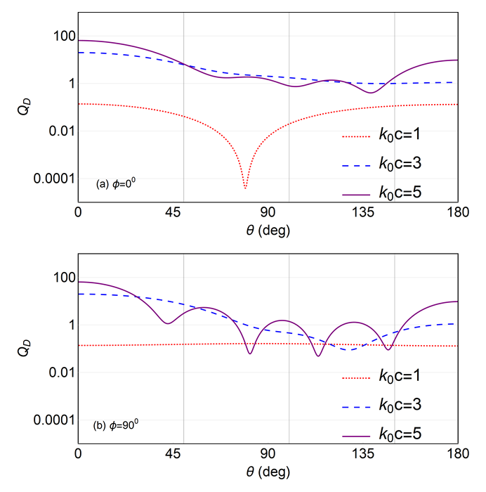
Figure 1: $Q_{D}(\theta,\phi)$ vs. $\theta$ for a biaxially dielectric-magnetic ellipsoid when $\hat{\mathbf{k}}_{inc}=\hat{\mathbf{z}}$ and $\hat{\mathbf{e}}_{inc}=\hat{\mathbf{x}}$; $\varepsilon_{r}=4$, $\mu_{r}=1.1$, $a/c=1/2$, $b/c=2/3$, $\alpha_{x}=1.1$, and $\alpha_{y}=1.2$. The red dotted lines represent ${k_{\scriptscriptstyle 0}}c=1$, the blue dashed lines ${k_{\scriptscriptstyle 0}}c=3$, and the purple solid lines ${k_{\scriptscriptstyle 0}}c=5$. (a) $\phi=0^{\circ}$, (b) $\phi=90^{\circ}$.

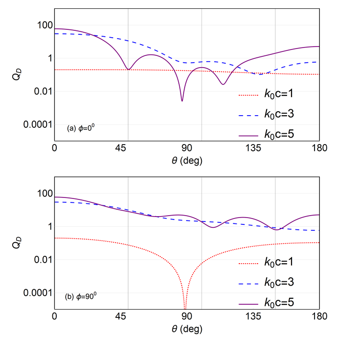
Figure 2: Same as Fig. 1, but when $\hat{\mathbf{e}}_{inc}=\hat{\mathbf{y}}$.

Scattering patterns for $\phi\in\left\{0^{\circ},90^{\circ}\right\}$ and ${k_{\scriptscriptstyle 0}}c\in\left\{1,3,5\right\}$ of the chosen biaxially dielectric-magnetic ellipsoid are depicted in Figs. 1 and 2. When ${k_{\scriptscriptstyle 0}}c$ is small, the sole null of $Q_{D}(\theta,\phi)$ occurs close to $\theta=90^{\circ}$ in Figs. 1(a) and 2(b). This null can be attributed to the electric-dipole terms in Eqs. (18) and (19). The contributions of the magnetic-dipole terms are much smaller because $\mu_{r}$ is much closer to unity than $\varepsilon_{r}$ is; indeed, on interchanging the values of $\varepsilon_{r}$ and $\mu_{r}$, we found the null to occur in Figs. 1(b) and 2(a). The contributions of the higher-order multipole terms are vanishingly small because ${k_{\scriptscriptstyle 0}}c$ is sufficiently small. We have verified that the null identified in Figs. 1(a) and 2(b) occurs exactly at $\theta=90^{\circ}$ when ${k_{\scriptscriptstyle 0}}c<0.1$, just as for a biaxially dielectric-magnetic sphere [28]. As the electrical size of the scattering object increases, the formation of lobes in the scattering pattern is evident from the presence of multiple nulls in these figures, just like for isotropic-dielectric objects [15, 16, 22, 38]. The foregoing remarks also apply to the scattering patterns of the chosen uniaxially dielectric-magnetic spheroid shown in Fig. 3.

A feature expected for the biaxially dielectric-magnetic ellipsoid is that the scattering patterns for

• $\phi=0^{\circ}$ when $\hat{\mathbf{e}}_{inc}=\hat{\mathbf{x}}$ and

• $\phi=90^{\circ}$ when $\hat{\mathbf{e}}_{inc}=\hat{\mathbf{y}}$

do not coincide. This expectation, which emerges both from the ellipsoidal shape of the object and its constitutive anisotropy, is borne out in Figs. 1(a) and 2(b). For the same reasons, the scattering patterns for $\phi=0^{\circ}$ in Fig. 2(a) do not coincide with the scattering patterns for $\phi=90^{\circ}$ in Fig. 1(b). As both $a=b$ and $\alpha_{x}=\alpha_{y}$ for the uniaxially dielectric-magnetic spheroid, neither of the two features is exhibited by the scattering patterns in Fig. 3.

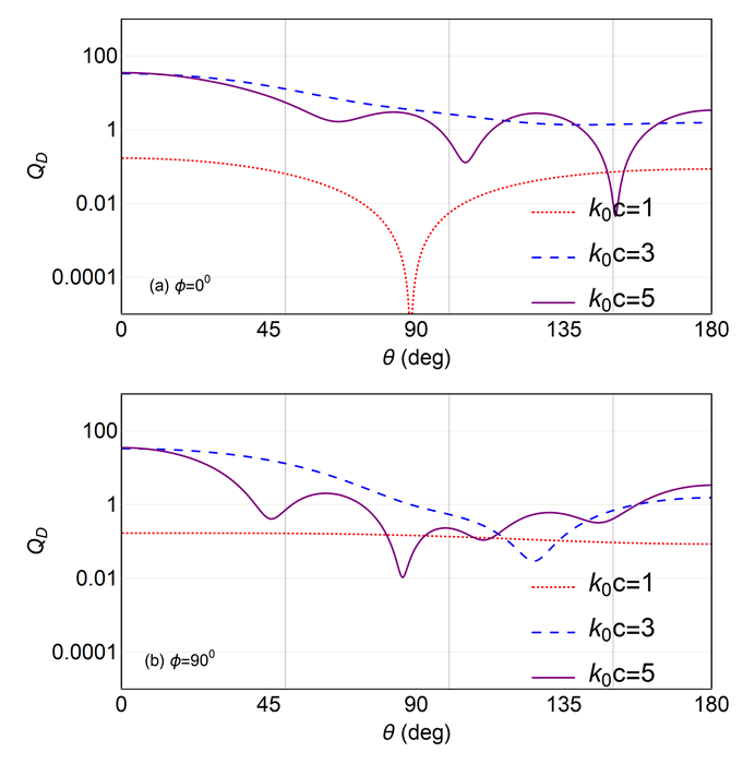
Figure 3: $Q_{D}(\theta,\phi)$ vs. $\theta$ for a uniaxially dielectric-magnetic spheroid when $\hat{\mathbf{k}}_{inc}=\hat{\mathbf{z}}$; $\varepsilon_{r}=4$, $\mu_{r}=1.1$, $a/c=b/c=1/2$, and $\alpha_{x}=\alpha_{y}=1.1$. The red lines represent ${k_{\scriptscriptstyle 0}}c=1$, the blue lines ${k_{\scriptscriptstyle 0}}c=3$, and the purple lines ${k_{\scriptscriptstyle 0}}c=5$. (a) Either $\left\{\phi=0^{\circ},\hat{\mathbf{e}}_{inc}=\hat{\mathbf{x}}\right\}$ or $\left\{\phi=90^{\circ},\hat{\mathbf{e}}_{inc}=\hat{\mathbf{y}}\right\}$. (b) Either $\left\{\phi=90^{\circ},\hat{\mathbf{e}}_{inc}=\hat{\mathbf{x}}\right\}$ or $\left\{\phi=0^{\circ},\hat{\mathbf{e}}_{inc}=\hat{\mathbf{y}}\right\}$.

3.2 Total scattering and absorption efficiencies

The total scattering efficiency $Q_{sca}$ and the absorption efficiency $Q_{abs}$ are plotted in Fig. 4 as functions of ${k_{\scriptscriptstyle 0}}c$ for a biaxial dielectric-magnetic ellipsoid described by $\varepsilon_{r}=2(1+0.1i)$, $\mu_{r}=1.05$, $\alpha_{x}=1.1$, $\alpha_{y}=1.2$, $a/c=1/2$, and $b/c=2/3$. These results are shown for all six canonical configurations of the incident plane wave with respect to the semi-axes of the ellipsoid; i.e., $\hat{\mathbf{k}}_{inc}\in\left\{\hat{\mathbf{x}},\hat{\mathbf{y}},\hat{\mathbf{z}}\right\}$ and $\hat{\mathbf{e}}_{inc}\in\left\{\hat{\mathbf{x}},\hat{\mathbf{y}},\hat{\mathbf{z}}\right\}$ such that $\hat{\mathbf{k}}_{inc}\perp\hat{\mathbf{e}}_{inc}$.

Clearly, $Q_{sca}<Q_{abs}$ when $\hat{\mathbf{k}}_{inc}=\hat{\mathbf{z}}$, regardless of the electrical size ${k_{\scriptscriptstyle 0}}c$ and the polarization state of the incident plane wave. Both $\hat{\mathbf{e}}_{inc}$ and $\hat{\mathbf{h}}_{inc}$ are then parallel to either $\hat{\mathbf{x}}$ or $\hat{\mathbf{y}}$, i.e.,

• neither to the eigenvector of $\underline{\underline{\varepsilon}}_{r}$ (also, $\underline{\underline{\mu}}_{r}$) corresponding to its eigenvalue with the largest magnitude

• nor to the eigenvector of $\underline{\underline{U}}$ corresponding to its largest eigenvalue.

Thus, $Q_{sca}<Q_{abs}$ for two canonical configurations of the incident plane wave in Fig. 4. Calculations for $c/a=2$ and $b/a=2/3$ (results not shown here) indicate that $Q_{sca}<Q_{abs}$ holds regardless of ${k_{\scriptscriptstyle 0}}c$ when $\hat{\mathbf{k}}_{inc}=\hat{\mathbf{x}}$. Thus, it would appear that $Q_{sca}<Q_{abs}$ when $\hat{\mathbf{k}}_{inc}$ is parallel to the eigenvector of $\underline{\underline{U}}$ corresponding to its largest eigenvalue. However, calculations for $\varepsilon_{r}=4(1+0.1i)$, $\mu_{r}=1.1$, $a/c=1/2$, and $b/c=2/3$ (results not shown here) indicate that the inequality $Q_{sca}<Q_{abs}$ depends on ${k_{\scriptscriptstyle 0}}c$, even when $\hat{\mathbf{k}}_{inc}=\hat{\mathbf{z}}$; indeed, that inequality holds for ${k_{\scriptscriptstyle 0}}c\leq 1.1$ when $\hat{\mathbf{e}}_{inc}=\hat{\mathbf{x}}$, and for ${k_{\scriptscriptstyle 0}}c\leq 1.4$ when $\hat{\mathbf{e}}_{inc}=\hat{\mathbf{y}}$.

The inequality $Q_{sca}<Q_{abs}$ does not hold in Fig. 4 when either $\hat{\mathbf{e}}_{inc}$ or $\hat{\mathbf{h}}_{inc}$ is aligned parallel to $\hat{\mathbf{z}}$, i.e., the eigenvector corresponding to the eigenvalues of $\underline{\underline{\varepsilon}}_{r}$, $\underline{\underline{\mu}}_{r}$, and $\underline{\underline{U}}$ with the largest magnitude. Indeed, $Q_{sca}>Q_{abs}$ for smaller ${k_{\scriptscriptstyle 0}}c$ when $\hat{\mathbf{e}}_{inc}=\hat{\mathbf{z}}$ but for larger ${k_{\scriptscriptstyle 0}}c$ when $\hat{\mathbf{h}}_{inc}=\hat{\mathbf{z}}$. Calculations for $\varepsilon_{r}=1.05$ and $\mu_{r}=2(1+0.1i)$ (results not shown here) indicate that $Q_{sca}>Q_{abs}$ for larger ${k_{\scriptscriptstyle 0}}c$ when $\hat{\mathbf{e}}_{inc}=\hat{\mathbf{z}}$ but for smaller ${k_{\scriptscriptstyle 0}}c$ when $\hat{\mathbf{h}}_{inc}=\hat{\mathbf{z}}$.

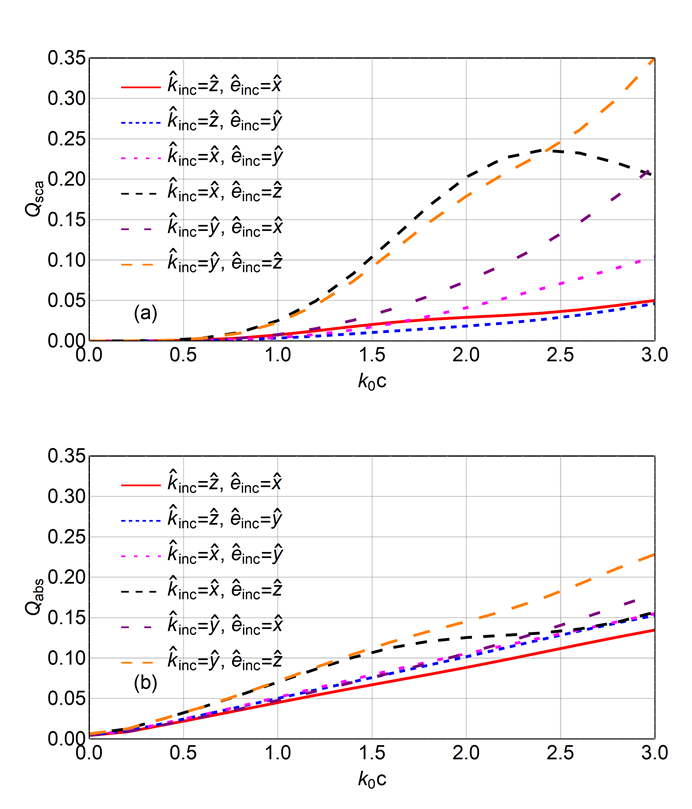
Figure 4: (a) $Q_{sca}$ and (b) $Q_{abs}$ vs. ${k_{\scriptscriptstyle 0}}c$ for a biaxially dielectric-magnetic ellipsoid; $\varepsilon_{r}=2(1+0.1i)$, $\mu_{r}=1.05$, $\alpha_{x}=1.1$, $\alpha_{y}=1.2$, $a/c=1/2$, and $b/c=2/3$.

In order to understand the effect of shape alone, we repeated the calculations for Fig. 4 but with $\varepsilon_{r}=1.68(1+0.1i)$, $\mu_{r}=0.882$, and $\alpha_{x}=\alpha_{y}=1$. Both $Q_{sca}$ and $Q_{abs}$ are plotted in Fig. 5 as functions of ${k_{\scriptscriptstyle 0}}c$ for this isotropic dielectric-magnetic ellipsoid whose relative permittivity is the average of the three eigenvalues of the relative permittivity dyadic and whose relative permeability is the average of the three eigenvalues of the relative permeability dyadic used for Fig. 4. When $\hat{\mathbf{k}}_{inc}=\hat{\mathbf{z}}$, $Q_{sca}$ for the isotropic dielectric-magnetic ellipsoid is greater than $Q_{sca}$ for the biaxially dielectric-magnetic ellipsoid, regardless of the electrical size ${k_{\scriptscriptstyle 0}}c$. This inequality does not hold for all ${k_{\scriptscriptstyle 0}}c$ when either $\hat{\mathbf{e}}_{inc}=\hat{\mathbf{z}}$ or $\hat{\mathbf{h}}_{inc}=\hat{\mathbf{z}}$; i.e., the eigenvector corresponding to the eigenvalue of $\underline{\underline{U}}$ with the largest magnitude. This inequality breaks down for smaller ${k_{\scriptscriptstyle 0}}c$ when $\hat{\mathbf{e}}_{inc}=\hat{\mathbf{z}}$ but for larger ${k_{\scriptscriptstyle 0}}c$ when $\hat{\mathbf{h}}_{inc}=\hat{\mathbf{z}}$. This breakdown can only be attributed to $\underline{\underline{U}}\neq\underline{\underline{I}}$ because the material is isotropic. Finally, $Q_{abs}$ for the isotropic dielectric-magnetic ellipsoid does not differ significantly from $Q_{abs}$ for the biaxially dielectric-magnetic ellipsoid. That is, the shape has a much more appreciable impact on $Q_{sca}$ than on $Q_{abs}$.

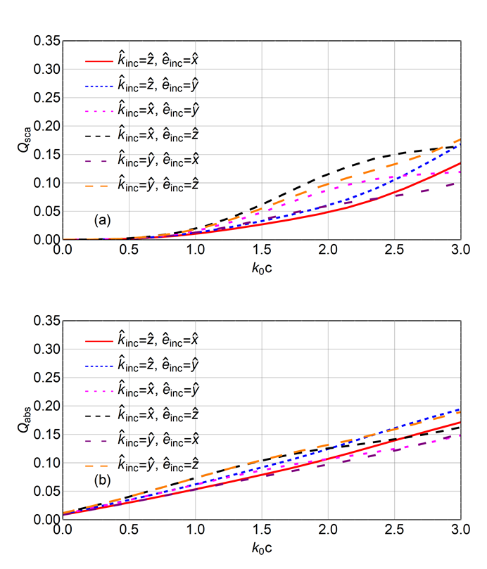
Figure 5: Same as Fig. 4, except that $\varepsilon_{r}=1.68(1+0.1i)$, $\mu_{r}=0.882$, and $\alpha_{x}=\alpha_{y}=1$.

3.3 Forward-scattering efficiency

For all six canonical configurations of the incident plane wave identified in Fig. 4 for a biaxially dielectric-magnetic ellipsoid, the forward-scattering efficiency $Q_{f}$ is almost a monotonically increasing function of ${k_{\scriptscriptstyle 0}}c\leq 3$. This is clear from Fig. 6 for $\varepsilon_{r}=2(1+0.1i)$, $\mu_{r}=1.05$, $\alpha_{x}=1.1$, $\alpha_{y}=1.2$, $a/c=1/2$, and $b/c=2/3$. The same conclusion was drawn for a uniaxially dielectric–magnetic spheroid with $\alpha_{x}=\alpha_{y}=1.1$ and $a/c=b/c=1/2$ (results not shown here).

Figure 6: $Q_{f}$ vs. ${k_{\scriptscriptstyle 0}}c$ for a biaxially dielectric-magnetic ellipsoid; $\varepsilon_{r}=2(1+0.1i)$, $\mu_{r}=1.05$, $\alpha_{x}=1.1$, $\alpha_{y}=1.2$, $a/c=1/2$, and $b/c=2/3$.

3.4 Backscattering efficiency

When $\hat{\mathbf{k}}_{inc}\in\left\{\hat{\mathbf{x}},\hat{\mathbf{y}}\right\}$, the backscattering efficiency $Q_{b}$ is almost a monotonically increasing function of ${k_{\scriptscriptstyle 0}}c\leq 3$, as shown in Fig. 7 for $\varepsilon_{r}=2(1+0.1i)$, $\mu_{r}=1.05$, $\alpha_{x}=1.1$, $\alpha_{y}=1.2$, $a/c=1/2$, and $b/c=2/3$. The same conclusion was drawn for a uniaxially dielectric–magnetic spheroid with $\alpha_{x}=\alpha_{y}=1.1$ and $a/c=b/c=1/2$ (results not shown here).

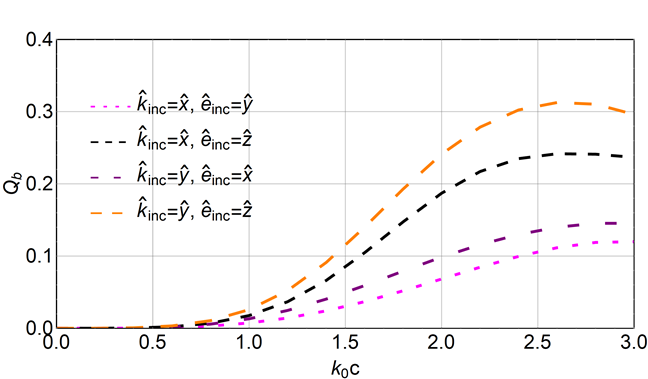
Figure 7: $Q_{b}$ vs. ${k_{\scriptscriptstyle 0}}c$ for a biaxially dielectric-magnetic ellipsoid when $\hat{\mathbf{k}}_{inc}\in\left\{\hat{\mathbf{x}},\hat{\mathbf{y}}\right\}$; $\varepsilon_{r}=2(1+0.1i)$, $\mu_{r}=1.05$, $\alpha_{x}=1.1$, $\alpha_{y}=1.2$, $a/c=1/2$, and $b/c=2/3$.

In Fig. 8, the variation of $Q_{b}$ with ${k_{\scriptscriptstyle 0}}c$ has an undulating character when $\hat{\mathbf{k}}_{inc}=\hat{\mathbf{z}}$. This is in contrast to the monotonic increase for $\hat{\mathbf{k}}_{inc}\in\{\hat{\mathbf{x}},\hat{\mathbf{y}}\}$ in Fig. 7.

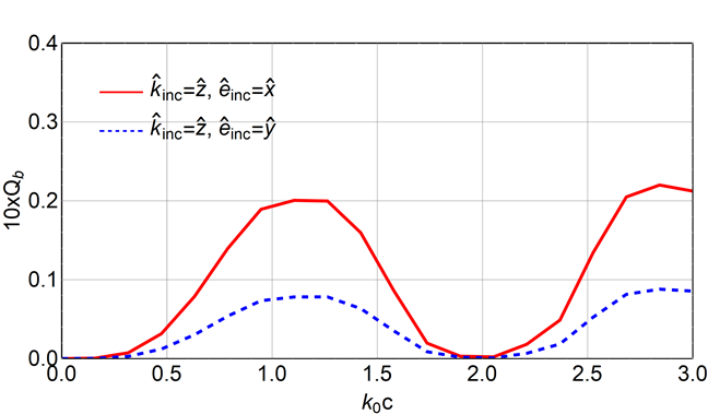
Figure 8: $Q_{b}$ vs. ${k_{\scriptscriptstyle 0}}c$ for a biaxially dielectric-magnetic ellipsoid when $\hat{\mathbf{k}}_{inc}=\hat{\mathbf{z}}$; $\varepsilon_{r}=2(1+0.1i)$, $\mu_{r}=1.05$, $\alpha_{x}=1.1$, $\alpha_{y}=1.2$, $a/c=1/2$, and $b/c=2/3$.

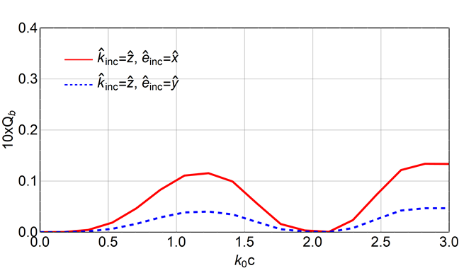
Figure 9: Same as Fig. 8 except that $a/c=b/c=1/2$.

The dependence of $Q_{b}$ in Fig. 8 on the polarization state of the incident plane wave is strong. Indeed, $Q_{b}$ for $\hat{\mathbf{e}}_{inc}=\hat{\mathbf{x}}$ exceeds $Q_{b}$ for $\hat{\mathbf{e}}_{inc}=\hat{\mathbf{y}}$. This must be due to both the shape ($a<b$) and the constitutive anisotropy ($\alpha_{x}<\alpha_{y}$) of the scattering object. When $\alpha_{y}<\alpha_{x}$ (results not shown here), $Q_{b}$ for $\hat{\mathbf{e}}_{inc}=\hat{\mathbf{y}}$ exceeds $Q_{b}$ for $\hat{\mathbf{e}}_{inc}=\hat{\mathbf{x}}$. Furthermore, when $b<a$ (results not shown here), $Q_{b}$ for $\hat{\mathbf{e}}_{inc}=\hat{\mathbf{x}}$ exceeds $Q_{b}$ for $\hat{\mathbf{e}}_{inc}=\hat{\mathbf{y}}$. Together, these data indicate that the constitutive anisotropy has a more significant impact than shape on $Q_{b}$.

The backscattering efficiency reduces in Fig. 9 when both $a/c$ and $b/c$ are equal to $1/2$ but $\alpha_{x}<\alpha_{y}$, but $Q_{b}$ for $\hat{\mathbf{e}}_{inc}=\hat{\mathbf{x}}$ still exceeds $Q_{b}$ for $\hat{\mathbf{e}}_{inc}=\hat{\mathbf{y}}$. The backscattering efficiency also reduces in Fig. 10 when both $\alpha_{x}$ and $\alpha_{y}$ are equal to $1.1$ but $a<b$, but now $Q_{b}$ for $\hat{\mathbf{e}}_{inc}=\hat{\mathbf{x}}$ is somewhat lower than $Q_{b}$ for $\hat{\mathbf{e}}_{inc}=\hat{\mathbf{y}}$. When $b<a$ (results not shown here), however, $Q_{b}$ for $\hat{\mathbf{e}}_{inc}=\hat{\mathbf{y}}$ becomes somewhat lower than $Q_{b}$ for $\hat{\mathbf{e}}_{inc}=\hat{\mathbf{x}}$. Finally, when both $\alpha_{x}=\alpha_{y}=1.1$ and $a/c=b/c=1/2$, the scattering object becomes a uniaxially dielectric-magnetic spheroid and $Q_{b}$ does not depend on the polarization state of the incident plane wave.

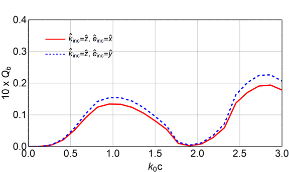
Figure 10: Same as Fig. 8 except that $\alpha_{x}=\alpha_{y}=1.1$.

Figure 11: Same as Fig. 8 except that $\alpha_{x}=\alpha_{y}=1.1$ and $a/c=b/c=1/2$.

One common observation in all the foregoing results for $\hat{\mathbf{k}}_{inc}=\hat{\mathbf{z}}$ is that the backscattering efficiency reduces to a very small value when ${k_{\scriptscriptstyle 0}}c=2$. Zero backscattering efficiency has been previously reported for isotropic dielectric-magnetic bodies of revolution when the incident plane wave propagates parallel to the axis of revolution and the scattering object is impedance matched to the free space surrounding it [48, 49]. However, for Figs. 8–11, the scattering object is not necessarily a body of revolution, it is not isotropic, and it is not impedance matched to free space. Scattering objects exhibiting $Q_{b}\to 0$ but large $Q_{f}$ hold promise to enhance the detection and harvesting of incident electromagnetic energy [50].

4 Concluding Remarks

We used the extended boundary condition method to study planewave scattering by a nonspherical object composed of an orthorhombic dielectric-magnetic material whose relative permittivity dyadic is a scalar multiple of its relative permeability dyadic. Numerical results were obtained for scattering by ellipsoids with semi-axes aligned parallel to the eigenvectors of the relative permittivity dyadic, hence allowing us to understand the relative impacts of constitutive anisotropy and nonsphericity.

Regardless of the direction of propagation and the polarization state of the incident plane wave, the adequate number of terms in the expansions of the scattered field phasors increase as the electrical size of the ellipsoid increases; as a result, more lobes appear in the scattering patterns. In this respect, constitutive anisotropy cannot be distinguished from isotropy. However, constitutive anisotropy is inimical to symmetry in scattering patterns.

The absorption efficiency can be either smaller or larger than the total scattering efficiency, depending on the electrical size of the scattering object, the ratio $\varepsilon_{r}/\mu_{r}$, and the direction of propagation and the polarization state of the incident plane wave. The shape of the scatterer has a more pronounced impact on the total scattering efficiency than on the absorption efficiency.

Regardless of the configuration of the incident plane wave, the forward scattering efficiency increases monotonically with the electrical size. The same characteristic is displayed by the backscattering efficiency for some, but not all, planewave configurations. For other configurations, the backscattering efficiency has an undulating behavior with increase in electrical size, and is highly affected by the shape and the constitutive anisotropy of the ellipsoid. The backscattering efficiency can be minuscule even when the forward-scattering efficiency is not, a desirable feature for harvesting incident electromagnetic energy. Minuscule backscattering can also provide immunity from detection by monostatic detection systems.

Acknowledgment. AL thanks the Charles Godfrey Binder Endowment at Penn State for ongoing support of his research activities.

Appendix

The polarizability dyadic of an electrically small biaxial-dielectric ellipsoid in vacuum is analytically known [37]. Accordingly,

• the polarizability dyadic of an electrically small sphere of radius $R$ composed of a material with relative permittivity dyadic $\varepsilon_{r}^{x}\,\hat{\mathbf{{\bf x}}}\hat{\mathbf{{\bf x}}}+\varepsilon_{r}^{y}\,\hat{\mathbf{{\bf y}}}\hat{\mathbf{{\bf y}}}+\varepsilon_{r}^{z}\,\hat{\mathbf{{\bf z}}}\hat{\mathbf{{\bf z}}}$ and

• the polarizability dyadic of an electrically small ellipsoid of semi-axes $a$, $b$, and $c$ and composed of a material with relative permittivity scalar $\varepsilon_{r}$

are identical, provided that

$$R^{3}=abc$$ (60)

and

$$\left.\begin{array}[]{l}\varepsilon_{r}^{x}=\displaystyle{\frac{\varepsilon_{r}\left(3L_{x}+2\right)+1-3L_{x}}{\varepsilon_{r}\left(3L_{x}-1\right)+4-3L_{x}}}\\[8.0pt] \varepsilon_{r}^{y}=\displaystyle{\frac{\varepsilon_{r}\left(3L_{y}+2\right)+1-3L_{y}}{\varepsilon_{r}\left(3L_{y}-1\right)+4-3L_{y}}}\\[8.0pt] \varepsilon_{r}^{z}=\displaystyle{\frac{\varepsilon_{r}\left(3L_{z}+2\right)+1-3L_{z}}{\varepsilon_{r}\left(3L_{z}-1\right)+4-3L_{z}}}\end{array}\right\}\,,$$ (61)

where [51, 52]

$$\left.\begin{array}[]{l}L_{x}=\displaystyle{\frac{abc}{2}\int_{0}^{\infty}\frac{dq}{(q+a^{2})^{3/2}(q+b^{2})^{1/2}(q+c^{2})^{1/2}}}\\[10.0pt] L_{y}=\displaystyle{\frac{abc}{2}\int_{0}^{\infty}\frac{dq}{(q+a^{2})^{1/2}(q+b^{2})^{3/2}(q+c^{2})^{1/2}}}\\[10.0pt] L_{z}=\displaystyle{\frac{abc}{2}\int_{0}^{\infty}\frac{dq}{(q+a^{2})^{1/2}(q+b^{2})^{1/2}(q+c^{2})^{3/2}}}\end{array}\right\}\,.$$ (62)

Analogously [37],

• the magnetizability dyadic [53, 54, 55] of an electrically small sphere of radius $R$ composed of a material with relative permeability dyadic $\mu_{r}^{x}\,\hat{\mathbf{{\bf x}}}\hat{\mathbf{{\bf x}}}+\mu_{r}^{y}\,\hat{\mathbf{{\bf y}}}\hat{\mathbf{{\bf y}}}+\mu_{r}^{z}\,\hat{\mathbf{{\bf z}}}\hat{\mathbf{{\bf z}}}$ and

• the magnetizability dyadic of an electrically small ellipsoid of semi-axes $a$, $b$, and $c$ and composed of a material with relative permeability scalar $\mu_{r}$

are identical, provided that Eq. (60) and conditions analogous to Eqs. (61) and (62) hold.

References

- [1] D. W. Thompson, On Growth and Form (Cambridge Univ. Press, 1942).
- [2] H. E. Stanley and N. Ostrowsky, eds., On Growth and Form: Fractal and Non-Fractal Patterns in Physics (Martinus Nijhoff, 1986)
- [3] C. Klein and C. S. Hurlbut Jr., Manual of Mineralogy 20th edn. (Wiley, 1985).
- [4] J. I. Gersten and F. W. Smith, The Physics and Chemistry of Materials (Wiley, 2001).
- [5] T. G. Mackay and A. Lakhtakia, Electromagnetic Anisotropy and Bianisotropy (World Scientific, 2010).
- [6] F. J. Molster and L. B. F. M. Waters, “The mineralogy of interstellar and circumstellar dust,” in Astromineralogy, T. K. Henning, ed. (Springer, 2003), pp. 121–170.
- [7] B. T. Draine, “Interstellar dust,” in Origin and Evolution of the Elements, A. McWilliams and M. Rauch, eds. (Cambridge U. Press, 2004), pp. 317–335.
- [8] I. N. Sokolik and O. B. Toon, “Incorporation of mineralogical composition into models of the radiative properties of mineral aerosol from UV to IR wavelengths,” J. Geophys. Res.: Atmos. 104, 9423–9444 (1999).
- [9] N. M. Estakhri and A. Alù, “Minimum-scattering superabsorbers,” Phys. Rev. B 89, 121416 (2014).
- [10] R. A. Dudley and M. A. Fiddy, Engineered Materials and Metamaterials: Design and Fabrication (SPIE, 2017).
- [11] X. C. Tong, Functional Metamaterials and Metadevices (Springer, 2018).
- [12] H. C. van de Hulst, Light Scattering by Small Particles (Dover Publications, 1957).
- [13] C. É. Kriegler, M. S. Rill, S. Linden, and M. Wegener, “Bianisotropic photonic metamaterials,” IEEE J. Sel. Top. Quantum Electron. 16, 367–375 (2010).
- [14] T. G. Mackay and A. Lakhtakia, Modern Analytical Electromagnetic Homogenization (Morgan & Claypool, 2015).
- [15] C. F. Bohren and D. R. Huffman, Absorption and Scattering of Light by Small Particles (Wiley, 1983).
- [16] J. J. Bowman, T. B. A. Senior, and P. L. E. Uslenghi, eds., Electromagnetic and Acoustic Scattering by Simple Shapes (North-Holland, 1969).
- [17] G. C. Hsiao, R. E. Kleinman, and D.-Q. Wang, “Applications of boundary integral equation methods in 3D electromagnetic scattering,” J. Comput. Appl. Math. 104, 89–110 (1999)
- [18] P. Ylä-Oijala, M. Taskinen, S. Järvenpää, “Surface integral equation formulations for solving electromagnetic scattering problems with iterative methods,” Radio Sci. 40, RS6002 (2005).
- [19] K. S. Kunz and R. S. Luebbers, The Finite Difference Time Domain Method for Electromagnetics (CRC Press, 1993).
- [20] P. B. Monk, Finite Element Methods for Maxwell’s Equations (Oxford University, 2003).
- [21] A. Lakhtakia, Beltrami Fields in Chiral Media (World Scientific, 1994).
- [22] S. Asano and G. Yamamoto, “Light scattering by a spheroidal particle,” Appl. Opt. 14, 29–49 (1975).
- [23] L.-W. Li, X.-K. Kang, and M.-S. Leong, Spheroidal Wave Functions in Electromagnetic Theory (Wiley, 2004).
- [24] P. C. Waterman, “Matrix formulation of electromagnetic scattering,” Proc. IEEE 53, 805–812 (1965).
- [25] A. Lakhtakia, “The Ewald–Oseen extinction theorem and the extended boundary condition method,” in The World of Applied Electromagnetics, A. Lakhtakia and C. M. Furse, eds. (Springer, 2018), pp. 481–513.
- [26] C.-T. Tai, Dyadic Green Functions in Electromagnetic Theory (IEEE Press, 1994).
- [27] A. Lakhtakia and T. G. Mackay, “Vector spherical wavefunctions for orthorhombic dielectric-magnetic material with gyrotropic-like magnetoelectric properties,” J. Opt. (India) 41, 201–213 (2012).
- [28] A. D. U. Jafri and A. Lakhtakia, “Scattering of an electromagnetic plane wave by a homogeneous sphere made of an orthorhombic dielectric-magnetic material,” J. Opt. Soc. Am. A 31, 89–100 (2014).
- [29] A. D. U. Jafri and A. Lakhtakia, “Scattering of an electromagnetic plane wave by a homogeneous sphere made of an orthorhombic dielectric-magnetic material: erratum,” J. Opt. Soc. Am. A 31, 2630 (2014).
- [30] P. M. Morse and H. Feshbach, Methods of Theoretical Physics, Vol. II (McGraw–Hill, 1953), pp. 1865–1866.
- [31] J. A. Stratton, Electromagnetic Theory (McGraw–Hill, 1941), pp. 564–565.
- [32] J. D. Jackson, Classical Electrodynamics 3rd edn. (Wiley, 1999), Sec. 9.7.
- [33] Y. Jaluria, Computer Methods for Engineering (Taylor & Francis, 1996), Sec. 7.5.3.
- [34] I. S. Gradshteyn and I. M. Ryzhik, Table of Integrals, Series, and Products 7th edn. (Academic Press, 2007).
- [35] T. J. Garner, A. Lakhtakia, J. K. Breakall, and C. F. Bohren, “Lorentz invariance of absorption and extinction cross sections of a uniformly moving object,” Phys. Rev. A 96, 053839 (2017).
- [36] E. Kreyszig, Advanced Engineering Mathematics 10th edn. (Wiley, 2011), Sec. 20.2.
- [37] A. Lakhtakia, “Electromagnetic response of an electrically small bianisotropic ellipsoid immersed in a chiral fluid,” Ber. Bunsenges. Physik. Chem. 95, 574–576 (1991).
- [38] P. Barber and C. Yeh, “Scattering of electromagnetic waves by arbitrarily shaped dielectric bodies,” Appl. Opt. 14, 2864–2872 (1975).
- [39] M. F. Iskander, A. Lakhtakia, and C. H. Durney, “A new procedure for improving the solution stability and extending the frequency range of the EBCM,” IEEE Trans. Antennas Propagat. 31, 317–324 (1983).
- [40] M. F. Werby and L. H. Green, “An extended unitary approach for acoustical scattering from elastic shells immersed in a fluid,” J. Acoust. Soc. Am. 74, 625–630 (1983).
- [41] A. Lakhtakia, V. K. Varadan, and V. V. Varadan, “Scattering by lossy dielectric slender objects with nonvanishing magnetic susceptibility,” J. Appl. Phys. 56, 3057–3060 (1984).
- [42] L. Lewin, “On the restricted validity of point-matching techniques,” IEEE Trans. Microw. Theory Tech. 18, 1041–1047 (1970).
- [43] S. Lefschetz, Differential Equations: Geometric Theory (Wiley, 1963).
- [44] V. V. Varadan, A. Lakhtakia, and V. K. Varadan, “Comments on recent criticism of the T-matrix method,” J. Acoust. Soc. Am. 84, 2280–2284 (1988).
- [45] A. Lakhtakia, V. K. Varadan, and V. V. Varadan, “Scattering by highly aspherical targets: EBCM coupled with reinforced orthogonalizations,” Appl. Opt. 23, 3502–3504 (1984).
- [46] L. Bi, P. Yang, G. W. Kattawar, and M. I. Mishchenko, “Efficient implementation of the invariant imbedding T-matrix method and the separation of variables method applied to large nonspherical inhomogeneous particles,” J. Quant. Spectrosc. Radiat. Transfer 116, 169–183 (2013).
- [47] L. Bi and P. Yang, “Accurate simulation of the optical properties of atmospheric ice crystals with the invariant imbedding T-matrix method,” J. Quant. Spectrosc. Radiat. Transfer 138, 17–35 (2014).
- [48] R. J. Wagner and P. J. Lynch, “Theorem on electromagnetic backscatter,” Phys. Rev. 131, 21–23 (1963).
- [49] P. L. E. Uslenghi, “Three theorems on zero backscattering,” IEEE Trans. Antennas Propagat. 44, 269–270 (1996).
- [50] Y. Zhang, M. Nieto-Vesperinas, and J. J. Sáenz, “Dielectric spheres with maximum forward scattering and zero backscattering: a search for their material composition,” J. Opt. (Bristol) 17, 105612 (2015).
- [51] E. C. Stoner, “The demagnetizing factors for ellipsoids,” Phil. Mag. 36, 803–821 (1945).
- [52] J. A. Osborn, “Demagnetizing factors of the general ellipsoid,” Phys. Rev. 67, 351–357 (1945).
- [53] A. Lakhtakia and T. G. Mackay, “Size-dependent Bruggeman approach for dielectric-magnetic composite materials,” Arch. Elektr. Über. 59, 348–351(2005).
- [54] C. M. Krowne and J. Q. Shen, “Dressed-state mixed-parity transitions for realizing negative refractive index,” Phys. Rev. A 79, 023818 (2009).
- [55] A. Welter, R. E. Raab, and O. L. de Lange, “Translationally invariant semi-classical electrodynamics of magnetic media to electric octopole-magnetic quadrupole order,” J. Math. Phys. 54, 023512 (2013).