Exploring the Kondo effect of an extended impurity with chains of Co adatoms in a magnetic field

Abstract

Motivated by recent STM experiments, we explore the magnetic field induced Kondo effect that takes place at symmetry protected level crossings in finite Co adatom chains. We argue that the effective two-level system realized at a level crossing acts as an extended impurity coupled to the conduction electrons of the substrate by a distribution of Kondo couplings at the sites of the chain. Using auxiliary-field quantum Monte Carlo simulations, which quantitatively reproduce the field dependence of the zero-bias signal, we show that a proper Kondo resonance is present at the sites where the effective Kondo coupling dominates. Our modeling and numerical simulations provide a theoretical basis for the interpretation of the STM spectrum in terms of level crossings of the Co adatom chains.

The Kondo effect is one of the most extensively studied and adequately addressed many-body process occurring due to the screening of a local moment by a conduction electron cloud Hewson (1993); Kondo (1964); Wilson (1975). On the experimental side, recent advances in scanning tunneling microscopy (STM) open greater opportunities to realise and investigate the Kondo effect in various Kondo nanostructures Madhavan et al. (1998); Cronenwett et al. (1998); Park et al. (2002); Jarillo-Herrero et al. (2005); Wahl et al. (2005); Néel et al. (2011); Spinelli et al. (2015); Toskovic et al. (2016). For instance, the recent STM experiments on finite atomic spin-chain realizations of Co adatoms in the presence of an external magnetic field have revealed an interesting interplay between the Kondo problem and the physics of quantum spin chains in a field Toskovic et al. (2016). Co adatoms on a Cu₂N/Cu(100) surface carry a spin-3/2 with a strong uniaxial hard-axis anisotropy($D$) Otte et al. (2008); Spinelli et al. (2015), and applying an external magnetic field perpendicular to the surface, the Co adatom chain effectively behaves like a spin-1/2 XXZ chain in transverse field. The magnetic field induced level crossings of finite XXZ and SU(2) chains are similar so that the experiments of Ref. [Toskovic et al., 2016] can be discussed in the context of the SU(2) invariant version of the model:

$$\hat{H} = -t\sum_{\langle{\boldsymbol{i}},{\boldsymbol{j}}\rangle,\sigma}(\hat{c}^{\dagger}_{{\boldsymbol{i}},\sigma}\hat{c}_{{\boldsymbol{j}},\sigma}+h.c)+J_{k}\sum^{L}_{\boldsymbol{l}=1}\hat{\boldsymbol{S}}^{c}_{\boldsymbol{l}}\cdot\hat{\boldsymbol{S}}_{\boldsymbol{l}}$$ (1)

$$+J_{h}\sum^{L-1}_{\boldsymbol{l}=1}\hat{\boldsymbol{S}}_{\boldsymbol{l}}\cdot\hat{\boldsymbol{S}}_{\boldsymbol{l}+\Delta\boldsymbol{l}}-g\mu_{B}h^{\bf z}\sum^{L}_{\boldsymbol{l}=1}\hat{S}^{z}_{\boldsymbol{l}}.$$

Here, $t$ is the hopping parameter of the conduction electrons, $J_{k}$ the antiferromagnetic Kondo coupling between a Co adatom and the conduction electrons, $J_{h}$ the Heisenberg antiferromagnetic coupling, $h^{\bf z}$ an external magnetic field in the $z$ direction, $L$ the length of the Heisenberg chain, $\hat{\boldsymbol{S}}_{\boldsymbol{l}}$ spin-1/2 operators and $\hat{\boldsymbol{S}}^{c}_{\boldsymbol{l}}=\frac{1}{2}\sum_{\sigma,\sigma^{\prime}}\hat{c}^{\dagger}_{\boldsymbol{l},\sigma}\boldsymbol{\sigma}_{\sigma,\sigma^{\prime}}\hat{c}_{\boldsymbol{l},\sigma^{\prime}}$ denotes the spin of conduction electrons. Throughout the calculation we set $t,\mu_{B}=1$ and $g=2$.

When the Kondo coupling is switched off ($J_{k}=0$), the chain undergoes a series of level crossings that lead to steps in the magnetization curve. In the geometry used in the experiment of Ref. [Toskovic et al., 2016], $J_{h}$ and the Kondo energy $\epsilon_{k}=k_{B}T_{k}$ are both of the order of 0.2 meV, with two important consequences: There is a competition between the Heisenberg coupling and the Kondo effect, and one can reach the saturation field of the isolated chain.

The main result of the STM experiments of Ref. [Toskovic et al., 2016] is to demonstrate that the differential conductance exhibits a series of anomalies as a function of the field, and that these anomalies coincide with the fields at which the isolated chain is expected to undergo level crossings. These anomalies are strongly site dependent however. Occasionally they take the typical V-shape of the Kondo resonance of a single impurity split by a magnetic field, but in most cases they are less pronounced if at all.

In this Letter, our goal is to provide a theory of STM that is valid at low temperature and that puts the measurements in the appropriate Kondo context. As we shall see, a Kondo effect is indeed present at each level crossing, but it corresponds to that of an extended impurity of size the length of the chain. The Hilbert space of this extended impurity corresponds to the twofold degenerate ground state of the spin chain at the level crossing. The presence or absence of a Kondo resonance at a given Co site where the STM signal is recorded depends i) on a matrix element encoding the fact that the ground state of the spin chain is addressed at a given Co site, and ii) on the magnitude of the effective Kondo coupling between the extended impurity and the substrate at the considered Co location.

Method. At high temperatures, the differential conductance in the presence of the Kondo coupling can be calculated using perturbation theory. While the results reproduce the gross features of the experimental data, they are limited to a regime above the Kondo temperature, and cannot account for the details of the low temperature data of Ref. [Toskovic et al., 2016]. For a particle-hole symmetric conduction band, our model can be simulated with the auxiliary field quantum Monte Carlo (QMC) algorithm without encountering the negative sign problem. We have used the finite temperature algorithm Blankenbecler et al. (1981); White et al. (1989); Assaad and Evertz (2008) of the ALF-project Bercx et al. (2017) and followed Refs. [Assaad, 1999; Sato et al., 2018] for the implementation of our Kondo model. In the QMC calculation we consider a $20\times 20$ square lattice with unit lattice constant and hopping matrix element $t$ and consider a linear arrangement of magnetic adatoms at distance $\Delta\boldsymbol{l}=(0,3)$ or $\Delta\boldsymbol{l}=(3,2)$ from each other (up to $L=7$). To overcome the finite size effects we included an orbital magnetic field corresponding to a single flux quantum traversing the whole lattice Assaad (2002), and a rather large value of the Kondo interaction $J_{k}/t=2$ so as to ensure that the Kondo scale of the single impurity problem remains larger than the finite size level spacing of the conduction electrons. Finally we consider $J_{h}/t=1.8$.

In the case of a single adatom ($L=1$), the problem reduces to that of a single impurity. The low temperature STM signal observed in Ref. [Toskovic et al., 2016] consists of a single peak, the Kondo resonance, consistent with a tunneling process from sample to tip that goes through the localized d-orbital of the Co adatoms. To account for this in the realm of the Kondo model we compute co-tunneling processes Figgins and Morr (2010); Ternes (2015); Morr (2017) given by: $A_{\boldsymbol{l}}(\omega)=-\text{Im}G_{\boldsymbol{l}}^{\text{ret}}(\omega)$ with $G_{\boldsymbol{l}}^{\text{ret}}(\omega)=-i\int_{0}^{\infty}d\tau e^{i\omega\tau}\sum_{\sigma}\big{<}\big{\{}\tilde{d}_{\boldsymbol{l},\sigma}(\tau),\tilde{d}_{\boldsymbol{l},\sigma}^{\dagger}(0)\big{\}}\big{>}$ and $\tilde{d}_{\boldsymbol{l},\sigma}^{\dagger}=\hat{c}^{\dagger}_{\boldsymbol{l},-\sigma}\hat{S}^{\sigma}_{\boldsymbol{l}}+\sigma\hat{c}_{\boldsymbol{l},\sigma}^{\dagger}\hat{S}^{z}_{\boldsymbol{l}}$. Here $\sigma=\pm$ runs over the two spin polarization and $\hat{S}^{\pm}_{\boldsymbol{l}}=\hat{S}^{x}_{\boldsymbol{l}}\pm i\hat{S}^{y}_{\boldsymbol{l}}$. This form can be obtained by starting from the single impurity Anderson model and applying the canonical Schrieffer-Wolf transformation (see supplemental material of Ref. [Raczkowski and Assaad, 2019]) and agrees with the expression given in Ref. [Costi, 2000].

Let us start by showing examples of spectral functions at level crossings obtained from QMC by stochastic analytic continuation Beach (2004). As apparent from Fig. 1a), for a single impurity we observe the characteristic temperature dependence of a Kondo resonance at zero field.

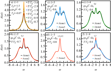
Figure 1: The spectral function computed using stochastic analytical continuation algorithm Beach (2004) at a given level crossings up to $L=4$. For $L>1$ we choose $J_{h}/t=1.8$ and $J_{k}/t=2$. The corresponding Kondo scale is extracted in Fig. 3.

Fig. 1 also shows the magnetic field induced Kondo resonances. For the two site chain there is a single level crossing between the singlet and the triplet at $g\mu_{B}h^{z}=\Delta_{1}^{0,1}$. In the generic Kondo problem, time reversal symmetry protects the two-fold degeneracy of the impurity state. Here parity protects the level crossings and a Kondo resonance is apparent on both adatom sites, see Fig. 1b). For the three site chain two level crossings occur before saturation. The ground state is a spin-1/2 doublet in zero field and resonances are seen on the first and third adatoms, see Fig. 1c). At the second level crossing, the resonance is seen only on the central adatom, see Fig. 1d). For $L=4$, Kondo resonances emerge on outer adatoms at the first level crossing, see Fig.1e), and on the central adatoms for the second level crossing, see Fig. 1.f).

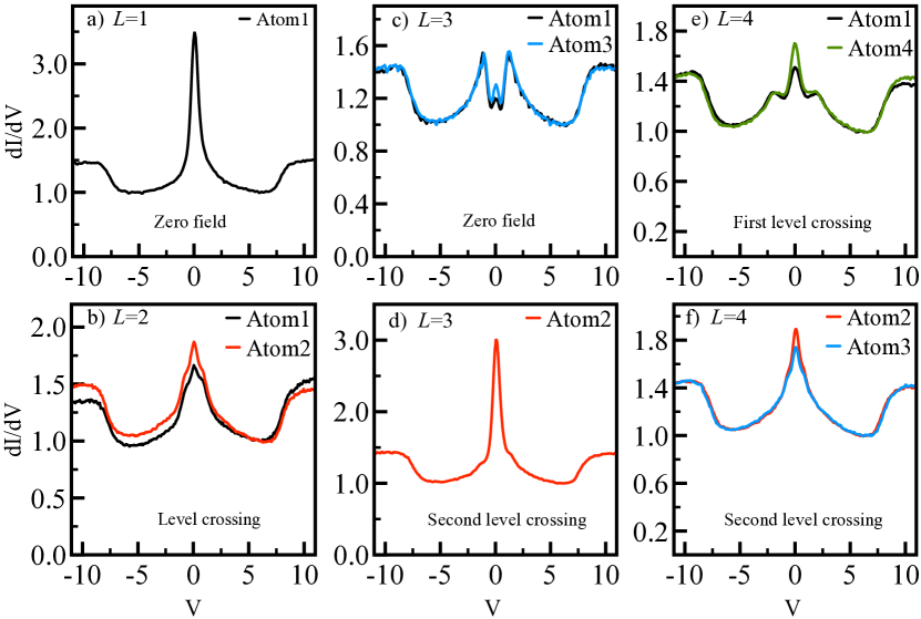
Figure 12: Differential conductance (in atomic units) as a function of voltage measured in STM experiment of Ref. [Toskovic et al., 2016].

These results have been obtained at temperatures already representative of the low temperature regime, and they reproduce the main features of the experimental results (see Supplemental Material, Ref. [sup, ], Fig. 12). However, to make a quantitative comparison with the experiments, which correspond to much lower temperature, we will concentrate on the zero bias differential conductance measured in the STM experiment Spinelli et al. (2015); Toskovic et al. (2016); Otte et al. (2008) as

$$dI_{\boldsymbol{l}}/dV(V=0)=2\frac{e^{2}}{\hbar}\int^{\infty}_{-\infty}d\omega\Big{(}-\frac{df(\omega)}{d\omega}\Big{)}A_{\boldsymbol{l}}(\omega)$$ (2)

where $f(\omega)$ is a Fermi function. In the low temperature limit the above maps onto:

$$dI_{\boldsymbol{l}}/dV(V=0)\simeq 2\frac{e^{2}}{\hbar}A_{\boldsymbol{l}}(\omega=0)\simeq 2\frac{e^{2}}{\pi\hbar}\beta G_{\boldsymbol{l}}(\tau=\beta/2)$$ (3)

where $G_{\boldsymbol{l}}(\tau)=\sum_{\sigma}\langle\tilde{d}_{\boldsymbol{l},\sigma}(\tau)\tilde{d}_{\boldsymbol{l},\sigma}^{\dagger}(0)\rangle$ is the imaginary time Green function which can be directly computed in the auxiliary field QMC. This approach avoids analytical continuation and our discussion will be based on the field dependence of this quantity. In the zero temperature limit the above equation is exact, and a more precise account of the zero bias differential conductance at finite temperature without using the analytical continuation can be obtained following Refs. [Luitz et al., 2012; Karrasch et al., 2010; Monien, 2010].

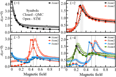
Figure 2: The $\tilde{d}$-spectral function at $\omega=0$ computed by QMC for a Heisenberg chain in a field together with the zero bias conductance measured in the STM experiment (in atomic units) for an XXZ chain in transverse field Toskovic et al. (2016). The magnetic field axis is normalised by the maximum values in both cases. The continuous grey vertical lines and the dashed grey lines denote the expected exact positions of the level crossings for a Heisenberg chain and for an XXZ one Toskovic et al. (2016), respectively.

The QMC results of the local spectral function at zero frequency for $k_{B}T/t=1/30$ are compared to the zero bias conductance reported in Ref. [Toskovic et al., 2016] as a function of external magnetic field in Fig. 2. Noticeably, up to four atoms the zero frequency spectral function shows excellent agreement with the corresponding zero bias conductance measured in the experiment. The temperature scales in the QMC and STM are comparable: the data presented in Fig. 2 are computed below $k_{B}T^{l}_{k}/8t$, where $T^{l}_{k}$ is an estimate of Kondo temperature from scaling of local spin susceptibility Hirsch and Fye (1986); Assaad (2002) at each level crossings (see below), while the STM data are taken at $330$ mK $\sim T^{Co}_{k}/8$ ($k_{B}T/t\sim 1/35$ in QMC).

To associate an adatom dependent Kondo temperature to each level crossing, we compute the local transverse susceptibility, $\chi_{\boldsymbol{l}}=\int^{\beta}_{0}d\tau\langle\hat{S}^{+}_{\boldsymbol{l}}(\tau)\hat{S}^{-}_{\boldsymbol{l}}(0)+h.c\rangle$, where $\hat{S}^{\pm}_{\boldsymbol{l}}(\tau)=e^{\tau\hat{H}}\hat{S}^{\pm}_{\boldsymbol{l}}e^{-\tau\hat{H}}$. Interestingly we observe in Fig. 3 that when the STM data at an adatom site shows a resonance, the local susceptiblity follows the expected universal behaviour, $T\chi_{l}=f(T/T^{l}_{k})$, where $T^{l}_{k}$ corresponds to the adatom and level crossing resolved Kondo temperature.

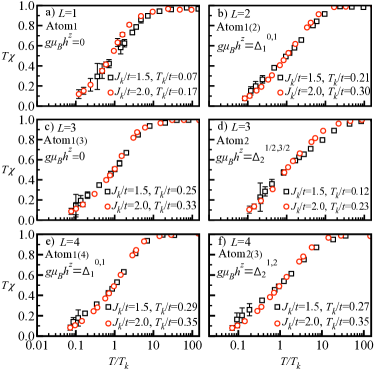
Figure 3: Local probe transverse susceptibility as a function of temperature computed for $J_{h}/t=1.8$ up to $L=4$ at sites where the level crossing leads to a Kondo resonance. The sites not shown do not follow the typical temperature dependence on Kondo couplings up to $k_{B}T/t\approx 1/40$.

Fig. 4 plots the temperature dependence of the zero frequency spectral function as estimated by $A_{\boldsymbol{l}}(\omega=0)\simeq\frac{1}{\pi}\beta G_{\boldsymbol{l}}(\tau=\beta/2)$. For $L=3$ and $L=4$ strong site dependence of the signal emerges below the Kondo temperature. We first concentrate on cases where we observe a dominant resonance. For these cases, the temperature dependence of the zero-bias conductance at the various sites (see Fig. 4) shows logarithmic increase at the Kondo scale upon reducing the temperature. At the other sites no such increase is observed. Quite remarkably, depending on the site, level crossings can show up as a peak, a dip, or a change of slope as a function of field. Accordingly, in the experimental results of Ref. [Toskovic et al., 2016], the frequency dependence at a critical field may or may not show a Kondo resonance.

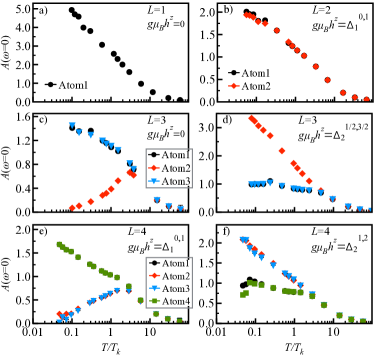
Figure 4: Exact zero-bias conductance as a function of temperature normalised by the corresponding Kondo scale at each level crossings up to $L=4$.

Effective model. To provide an effective model for a given level crossing, $p$, we project the Hamiltonian on the two fold degenerate Hilbert space of the level crossing. Clearly such a strategy is valid only if the gap separating the next excited states of the spin chain is large compared to the effective Kondo scale. For our SU(2) model, this approximation will necessarily fail in the large $L$ limit, but as we will see below it provides an accurate account of the QMC data for small $L$. Let $\{|{\mathbf{{\it m}_{1}}}\rangle=|\textbf{S}_{\mathbf{{\it m}_{1}}}\textbf{S}^{z}_{\mathbf{{\it m}_{1}}}\rangle_{p},|{\mathbf{{\it m}_{2}}}\rangle=|\textbf{S}_{\mathbf{{\it m}_{2}}}\textbf{S}^{z}_{\mathbf{{\it m}_{2}}}\rangle_{p}\}$ be the eigenstate of the Heisenberg chain with energies $e_{m_{1},p}$ , $e_{m_{2},p}$ that span the Hilbert space of the level crossing and $\hat{P}$ the projector onto this space. Defining a vector of Pauli spin matrices $\boldsymbol{\tau}$ that act on this Hilbert space, the projected Hamiltonian, up to a constant, reads:

$$\hat{H}^{eff}_{p}=-t\sum_{\langle{\boldsymbol{i}},{\boldsymbol{j}}\rangle,\sigma}(\hat{c}^{\dagger}_{{\boldsymbol{i}},\sigma}\hat{c}_{{\boldsymbol{j}},\sigma}+h.c)+J_{k}\sum_{\boldsymbol{l}}\Big{\{}j^{\perp}_{\boldsymbol{l},p}(\hat{S}^{x,c}_{\boldsymbol{l}}\hat{\tau}^{x}+$$

$$\hat{S}^{y,c}_{\boldsymbol{l}}\hat{\tau}^{y})+j^{z}_{\boldsymbol{l},p}\hat{S}^{z,c}_{\boldsymbol{l}}\hat{\tau}^{z}+\mu_{\boldsymbol{l},p}S^{z,c}_{\boldsymbol{l}}+(\Delta^{{\mathbf{{\it m}_{1}}},{\mathbf{{\it m}_{2}}}}_{p}-g\mu_{B}h^{\bf z})\hat{n}\Big{\}}$$ (4)

The energy difference between the two local states is given by $\Delta^{{\mathbf{{\it m}_{1}}},{\mathbf{{\it m}_{2}}}}_{p}=e_{{\mathbf{{\it m}_{2}}},p}-e_{{\mathbf{{\it m}_{1}}},p}$, $\hat{n}=\frac{1}{2}(\hat{\mathbf{1}}+\hat{\tau}^{z})$, and the site dependent effective couplings and the effective magnetic field are defined as; $j^{\perp}_{\boldsymbol{l},p}=\langle{\mathbf{{\it m}_{2}}}|\hat{S}^{x,y}_{\boldsymbol{l}}|{\mathbf{{\it m}_{1}}}\rangle$, $2j^{z}_{\boldsymbol{l},p}=-\langle{\mathbf{{\it m}_{1}}}|\hat{S}^{z}_{\boldsymbol{l}}|{\mathbf{{\it m}_{1}}}\rangle+\langle{\mathbf{{\it m}_{2}}}|\hat{S}^{z}_{\boldsymbol{l}}|{\mathbf{{\it m}_{2}}}\rangle$ and $2\mu_{\boldsymbol{l},p}=\langle{\mathbf{{\it m}_{1}}}|\hat{S}^{z}_{\boldsymbol{l}}|{\mathbf{{\it m}_{1}}}\rangle+\langle{\mathbf{{\it m}_{2}}}|\hat{S}^{z}_{\boldsymbol{l}}|{\mathbf{{\it m}_{2}}}\rangle$.

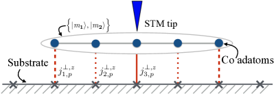
Figure 5: A chain of Co adatoms on a substrate implement, at a level crossing, the Kondo model of an extended impurity.

Table 1: Effective couplings $j^{\perp,z}_{\boldsymbol{l}(\boldsymbol{l}^{\prime}),p}$ at the level crossings($p=1,\cdots,\frac{L}{2}(\frac{L+1}{2})$ for a fixed even(odd) $L$.)

$L=2$	$j^{\perp}_{1(2),1}=\frac{1}{2\sqrt{2}}$,  $j^{z}_{1(2),1}=\frac{1}{4}$
$L=3$	$j^{\perp}_{1(3),1}=\frac{1}{3}$, $j^{\perp}_{2,1}=\frac{1}{6}$,  $j^{z}_{1(3),1}=\frac{1}{3}$,  $j^{z}_{2,1}=\frac{1}{6}$
$L=3$	$j^{\perp}_{1(3),2}=\frac{1}{2\sqrt{6}}$,  $j^{\perp}_{2,2}=\frac{1}{\sqrt{6}}$,  $j^{z}_{1(3),2}=\frac{1}{12}$, $j^{z}_{2,2}=\frac{1}{3}$
$L=4$	$j^{\perp}_{1(4),1}=\frac{1}{4\sqrt{6}{\sqrt{2+\sqrt{2}}}}\Big{[}\frac{1+\sqrt{2}}{1+\sqrt{3}}+1+\sqrt{1+\frac{\sqrt{3}}{2}}\big{(}1+\sqrt{2}\big{)}\Big{]}$
	$j^{\perp}_{2(3),1}=\frac{1}{4\sqrt{6}{\sqrt{2+\sqrt{2}}}}\Big{[}\frac{1}{1+\sqrt{3}}+(1+\sqrt{2})+\sqrt{1+\frac{\sqrt{3}}{2}}\Big{]}$
	$j^{z}_{1(4),1}=\frac{1}{16}(2+\sqrt{2})$,  $j^{z}_{2(3),1}=\frac{1}{16}(2-\sqrt{2})$
$L=4$	$j^{\perp}_{1(4),2}=\frac{1}{4{\sqrt{2+\sqrt{2}}}}$,  $j^{\perp}_{2(3),2}=\frac{1+\sqrt{2}}{4{\sqrt{2+\sqrt{2}}}}$
	$j^{z}_{1(4),2}=\frac{1}{16}(2-\sqrt{2})$,  $j^{z}_{2(3),2}=\frac{1}{16}(2+\sqrt{2})$

This model can be interpreted as the Kondo model of an extended impurity that is coupled to the conduction electrons at $L$ points (see Fig. 5). The projection does not affect the U(1) spin symmetry of the model, but as shown in Table 1 it yields a strong site dependence of the effective couplings $j^{\perp,z}_{\boldsymbol{l},p}$. To compute the co-tunneling within the effective model, we still have to project the spin operator onto the level-crossing Hilbert space $\hat{P}\tilde{d}_{\boldsymbol{l},\sigma}^{\dagger}\hat{P}=\hat{c}^{\dagger}_{\boldsymbol{l},-\sigma}\hat{P}\hat{S}^{\sigma}_{\boldsymbol{l}}\hat{P}+\sigma\hat{c}_{\boldsymbol{l},\sigma}^{\dagger}\hat{P}S^{z}_{\boldsymbol{l}}\hat{P}$ so that it acquires a site dependence when written in terms of $\boldsymbol{\tau}$ operators. This reflects the fact that in the experiment the extended states $| {\mathbf{{\it m}_{1}}}\rangle$ and $|{\mathbf{{\it m}_{2}}}\rangle$ are addressed via manipulation of one of the constituent Co d-spins. A detailed numerical analysis of the effective model along these lines is left for future studies. However, it is already clear that it provides a qualitative interpretation of the data in terms of a projection induced hierarchy of Kondo scales (see Ref. [sup, ], Table 4). Consider for instance the four-site chain at the first, $p=1$, level crossing for which $j^{z}_{1(4),1}/j^{z}_{2(3),1}=5.83$ and $j^{\perp}_{1(4),1}/j^{\perp}_{2(3),1}=1.25$. Thereby, the Kondo singlet will be predominantly formed by an entangled state of the degenerate two level system, $\left\{| {\mathbf{{\it m}_{1}}}\rangle,|{\mathbf{{\it m}_{2}}}\rangle\right\}$ and a symmetric combination of the conduction electron spins on sites one and four (see Ref. [sup, ], Section .2.). This provides an understanding of the observed Kondo like temperature dependence of the zero-bias conductance at sites one and four.

In Fig. 6 we consider chains up to seven spins. Here, an accurate comparison of the zero bias conductance is hard due to the asymmetric line shape of the Kondo resonances that arise in the experiment due to the potential scattering between tip and sample Figgins and Morr (2010); von Bergmann et al. (2015); Ternes (2015); Morr (2017), but a reasonable agreement can be achieved slightly away from the zero bias around $V\sim 0.4-0.8$ mV as shown in Fig. 6.

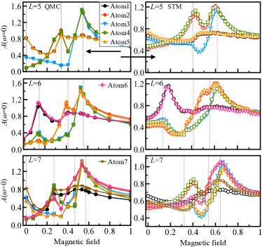
Figure 6: QMC results for five, six and seven atom spin-chains together with the STM data around $V\sim 0.6$ mV Toskovic et al. (2016) as a function of magnetic field (normalised by the maximum values).

As the chain size grows, the spectrum will collapse, and our understanding in terms of the projection onto the two-fold level crossing Hilbert space fails. In fact in this limit we expect a crossover to Kondo lattice behavior characterized at the mean field level by hybridized heavy and light bands in a magnetic field (see Ref. [sup, ], Section .3). For an infinite Heisenberg chain and within this approximation, we expect the conductance to reflect the local spinon density of states.

To summarize, we have shown that the STM measurements on Co adatom chains agree remarkably well with QMC simulations of a model of spin-1/2 chains in a field coupled to a conducting substrate via local Kondo couplings. To interpret the strong site dependence of the signal, we have performed a projection onto the symmetry protected level crossing Hilbert space of the spin chain that leads to the notion of an extended impurity with site dependent Kondo couplings. Consequently, screening happens via the dominant channel such that site and level crossing dependent Kondo resonances are observed in the STM co-tunneling conductance as well as in the Monte Carlo simulations. As a function of chain length, the above construction will progressively fail and we expect a crossover to Kondo lattice physics, in which the STM signal will pick up the two spinon continuum of the spin chain. Further work at understanding the details of the extended impurity Kondo model, as well as the crossover to the lattice limit is presently under progress.

Supplemental Material for: Exploring the Kondo effect of an extended impurity with chains of Co adatoms in a magnetic field

.1 Effective models at level crossings

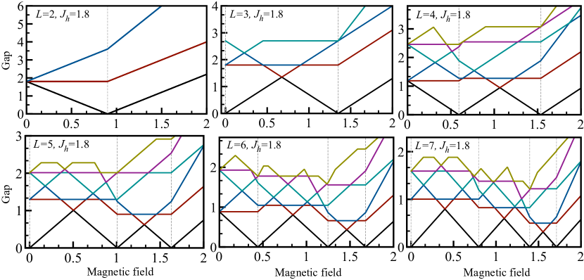
Figure 9: Lowest eigen energies as a function of magnetic field (in $z$-direction in units of $g\mu_{B}$) for a spin-1/2 Heisenberg chain.

Figure 10: Lowest energy excitations as a function of magnetic field (in $z$-direction in units of $g\mu_{B}$) for a spin-1/2 Heisenberg chain.

To derive the effective model at level crossing $p$ (see Fig. 10 and Fig. 10) we project the Hamiltonian of Eq. (1) onto the Hilbert space spanned by the states $\big{\{}|{\mathbf{{\it m}_{1}}}\rangle,|{\mathbf{{\it m}_{2}}}\rangle\big{\}}$ of the level crossing of a finite Heisenberg chain at a given critical magnetic field.

$$\hat{H}^{eff}_{p}=-t\sum_{\langle{\boldsymbol{i}},{\boldsymbol{j}}\rangle,\sigma}(\hat{c}^{\dagger}_{{\boldsymbol{i}},\sigma}\hat{c}_{{\boldsymbol{j}},\sigma}+h.c)+J_{k}\sum^{L}_{\boldsymbol{l}=1}\sum_{{\mathbf{{\it m}}}{\mathbf{{\it m^{\prime}}}}={\mathbf{{\it m}_{1}}},{\mathbf{{\it m}_{2}}}}\textbf{S}^{c}_{\boldsymbol{l}}\cdot|{\mathbf{{\it m^{\prime}}}}\rangle\langle{\mathbf{{\it m^{\prime}}}}|\textbf{S}_{\boldsymbol{l}}|{\mathbf{{\it m}}}\rangle\langle{\mathbf{{\it m}}}|$$

$$+(e_{{\mathbf{{\it m}_{1}}},p}-\textbf{S}^{z}_{{\mathbf{{\it m}_{1}}},p}h^{z})|{\mathbf{{\it m}_{1}}}\rangle\langle{\mathbf{{\it m}_{1}}}|+(e_{{\mathbf{{\it m}_{2}}},p}-\textbf{S}^{z}_{{\mathbf{{\it m}_{2}}},p}h^{z})|{\mathbf{{\it m}_{2}}}\rangle\langle{\mathbf{{\it m}_{2}}}|.$$ (5)

The states are explicitly given in Table 2.

Table 2: The subspace $\{|{\mathbf{{\it m}_{1}}}\rangle=|\textbf{S}_{\mathbf{{\it m}_{1}}}\textbf{S}^{z}_{\mathbf{{\it m}_{1}}}\rangle_{p},|{\mathbf{{\it m}_{2}}}\rangle=|\textbf{S}_{\mathbf{{\it m}_{2}}}\textbf{S}^{z}_{\mathbf{{\it m}_{2}}}\rangle_{p}\}$ at a level crossing $p$ of a finite Heisenberg chain ($J_{h}\sum^{L-1}_{\boldsymbol{l}=1}\hat{\boldsymbol{S}}_{l}\cdot\hat{\boldsymbol{S}}_{\boldsymbol{l}+1}$) and corresponding eigenenergies, lowest excitation gap, and effective magnetic field.

$L=2$	$|0\rangle=\frac{1}{\sqrt{2}}\left(\big{|}\uparrow\downarrow\rangle-|\downarrow\uparrow\big{\rangle}\right)$,  $\big{|}1\big{\rangle}=\big{|}\uparrow\uparrow\big{\rangle}$
	$e_{0,1}=-\frac{3}{4}J_{h}$,  $e_{1,1}=\frac{J_{h}}{4}$,  $\Delta^{0,1}_{1}=J_{h}$,  $\mu_{1(2),1}=\frac{1}{4}$
$L=3$	$\big{|}\frac{1}{2}\big{\rangle}=\frac{1}{\sqrt{6}}\big{(}|\downarrow\uparrow\uparrow\rangle-2|\uparrow\downarrow\uparrow\rangle+\uparrow\uparrow\downarrow\rangle\big{)}$,  $\big{|}-\frac{1}{2}\big{\rangle}=\frac{1}{\sqrt{6}}\left(|\downarrow\downarrow\uparrow\rangle-2|\downarrow\uparrow\downarrow\rangle+\uparrow\downarrow\downarrow\rangle\right)$
	$e_{\frac{1}{2},1}=-J_{h}$,  $e_{-\frac{1}{2},1}=-J_{h}$,  $\Delta^{-\frac{1}{2},\frac{1}{2}}_{1}=0$,  $\mu_{1(3),1}=0$,  $\mu_{2,1}=0$
$L=3$	$\big{|}\frac{1}{2}\big{\rangle}=\frac{1}{\sqrt{6}}\big{(}\big{|}\downarrow\uparrow\uparrow\big{\rangle}-2\big{|}\uparrow\downarrow\uparrow\big{\rangle}+\big{|}\uparrow\uparrow\downarrow\big{\rangle}\big{)}$,  $\big{|}\frac{3}{2}\big{\rangle}=\big{|}\uparrow\uparrow\uparrow\big{\rangle}$
	$e_{\frac{1}{2},2}=-J_{h}$,  $e_{\frac{3}{2},2}=\frac{J_{h}}{2}$,  $\Delta^{\frac{1}{2},\frac{3}{2}}_{2}=\frac{3}{2}J_{h}$,  $\mu_{1(3),2}=\frac{5}{12}$,  $\mu_{2,2}=\frac{1}{6}$
$L=4$	$\big{|}0\big{\rangle}=\frac{1}{\sqrt{6}}\Big{[}\frac{1}{(1+\sqrt{3})}\big{(}\big{|}\downarrow\downarrow\uparrow\uparrow\big{\rangle}+\big{|}\uparrow\uparrow\downarrow\downarrow\big{\rangle}\big{)}+\big{|}\downarrow\uparrow\uparrow\downarrow\big{\rangle}+\big{|}\uparrow\downarrow\downarrow\uparrow\big{\rangle}-\sqrt{1+\frac{\sqrt{3}}{2}}\big{(}\big{|}\downarrow\uparrow\downarrow\uparrow\big{\rangle}+\big{|}\uparrow\downarrow\uparrow\downarrow\big{\rangle}\big{)}\Big{]}$
	$\big{|}1\big{\rangle}=\frac{1}{2\sqrt{2+\sqrt{2}}}\Big{[}-\big{|}\downarrow\uparrow\uparrow\uparrow\big{\rangle}+\big{|}\uparrow\uparrow\uparrow\downarrow\big{\rangle}+(1+\sqrt{2})\big{(}\big{|}\uparrow\downarrow\uparrow\uparrow\big{\rangle}-|\uparrow\uparrow\downarrow\uparrow\big{\rangle}\big{)}\Big{]}$
	$e_{0,1}=\frac{J_{h}}{4}\big{(}-3-2\sqrt{3}\big{)}$, $e_{1,1}=\frac{J_{h}}{4}\big{(}-1-2\sqrt{2}\big{)}$,  $\Delta^{0,1}_{1}=\frac{J_{h}}{2}(1-\sqrt{2}+\sqrt{3})$, $\mu_{1(4),1}=\frac{(2+\sqrt{2})}{16}$, $\mu_{2(3),1}=\frac{(2-\sqrt{2})}{16}$
$L=4$	$\big{|}1\big{\rangle}=\frac{1}{2\sqrt{2+\sqrt{2}}}\Big{[}-\big{|}\downarrow\uparrow\uparrow\uparrow\big{\rangle}+\big{|}\uparrow\uparrow\uparrow\downarrow\big{\rangle}+(1+\sqrt{2})\big{(}\big{|}\uparrow\downarrow\uparrow\uparrow\big{\rangle}-\big{|}\uparrow\uparrow\downarrow\uparrow\big{\rangle}\big{)}\Big{]}$,   $\big{|}2\big{\rangle}=\big{|}\uparrow\uparrow\uparrow\uparrow\big{\rangle}$
	$e_{1,2}=\frac{J_{h}}{4}\big{(}-1-2\sqrt{2}\big{)}$, $e_{2,2}=\frac{3J_{h}}{4}$,  $\Delta^{1,2}_{2}=J_{h}\big{(}1+\frac{1}{\sqrt{2}}\big{)}$,  $\mu_{1(4),2}=\frac{(6+\sqrt{2})}{16}$, $\mu_{2(3),2}=\frac{(6-\sqrt{2})}{16}$

We further introduce pseudo spin-1/2 operators; $\hat{\tau}^{x}=|{\mathbf{{\it m}_{2}}}\rangle\langle{\mathbf{{\it m}_{1}}}|+|{\mathbf{{\it m}_{1}}}\rangle\langle{\mathbf{{\it m}_{2}}}|$, $\hat{\tau}^{y}=-i(|{\mathbf{{\it m}_{2}}}\rangle\langle{\mathbf{{\it m}_{1}}}|-|{\mathbf{{\it m}_{1}}}\rangle\langle{\mathbf{{\it m}_{2}}}|)$ and $\hat{\tau}^{z}=|{\mathbf{{\it m}_{2}}}\rangle\langle{\mathbf{{\it m}_{2}}}|-|{\mathbf{{\it m}_{1}}}\rangle\langle{\mathbf{{\it m}_{1}}}|$ and impose the constraint $\hat{\mathbf{1}}=|{\mathbf{{\it m}_{1}}}\rangle\langle{\mathbf{{\it m}_{1}}}|+|{\mathbf{{\it m}_{2}}}\rangle\langle{\mathbf{{\it m}_{2}}}|$. In terms of the $\boldsymbol{\tau}$ operators Eq. (5) takes the form given in Eq. (4) with a set of site dependent effective couplings given in Table 1. The other effective parameters of Eq. (4) are given in Table 2 up to L=4. When calculating the local matrix elements, we obtain an alternative $\pm$ sign of $j^{\perp}_{\boldsymbol{l},p}$ which does not affect Kondo physics Anderson et al. (1970); Anderson (1970). For simplicity we omitted this sign $(-1)^{\boldsymbol{l}}$ in Table 1 of the main text.

Noticeably, for a Heisenberg chain ($J_{h}\sum^{L-1}_{\boldsymbol{l}=1}\hat{\boldsymbol{S}}_{\boldsymbol{l}}\cdot\hat{\boldsymbol{S}}_{\boldsymbol{l}+1}$) the effective couplings $(j^{\perp,z}_{\boldsymbol{l}(\boldsymbol{l}^{\prime}),p})$ are independent of $J_{h}$ (see Table 1). However, for an XXZ chain ($J_{xy}\sum^{L-1}_{\boldsymbol{l}=1}(\hat{S^{x}}_{\boldsymbol{l}}\hat{S^{x}}_{\boldsymbol{l}+1}+\hat{S^{y}}_{\boldsymbol{l}}\hat{S^{y}}_{\boldsymbol{l}+1})+J_{zz}\sum^{L-1}_{\boldsymbol{l}=1}\hat{S^{z}}_{\boldsymbol{l}}\hat{S^{z}}_{\boldsymbol{l}+1}$) the ratio of the exchange parameters $J_{zz}/J_{xy}$ appears in the expression of the effective couplings. Since they do not have a simple form, we choose to plot them as a function of $J_{zz}/J_{xy}$ in Fig.8 and Fig.8 for chains of three and four atoms respectively. As for the Heisenberg chain ($J_{zz}/J_{xy}=1$), there is always a strong site dependence of the effective couplings when varying $J_{zz}/J_{xy}=0,\cdots,1$. Hence, the magnetic field induced level crossings in finite XXZ and Heisenberg chains is expected to show a similar site dependent Kondo physics.

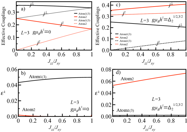
Figure 7: Top: Site dependent effective couplings as a function of $J_{zz}/J_{xy}$ at level crossings for $L=3$. Bottom: Corresponding effective Kondo scale as a function of $J_{zz}/J_{xy}$. Here, the effective Kondo scale is estimated as; $\epsilon^{k}_{l(l^{\prime}),p}\sim e^{-\frac{1}{j_{l,p}}}$ with $\frac{1}{\ j_{l,p}}=\frac{1}{\sqrt{(}{j^{\perp}_{l,p})^{2}-(j^{z}_{l,p})^{2}}}\times\tan^{-1}\Big{(}\frac{\sqrt{(j^{\perp}_{l,p})^{2}-(j^{z}_{l,p})^{2}}}{j^{z}_{l,p}}\Big{)}$ (see Section .2.).

Figure 8: Top: Site dependent effective couplings as a function of $J_{zz}/J_{xy}$ at level crossings for $L=4$. Bottom: Corresponding effective Kondo scale ($\epsilon^{k}_{l(l^{\prime}),p}\sim e^{-\frac{1}{j_{l,p}}}$) as a function of $J_{zz}/J_{xy}$.

.2 Effective Kondo Scale at level crossings (Anderson Poor man scaling approach)

Starting from the effective Kondo Hamiltonian for a chain of two atoms at singlet-triplet level crossing, which reads

$$\hat{H}^{eff}_{1} = e_{0,1}-t\sum_{\langle{\boldsymbol{i}},{\boldsymbol{j}}\rangle,\sigma}(\hat{c}^{\dagger}_{{\boldsymbol{i}},\sigma}\hat{c}_{{\boldsymbol{j}},\sigma}+h.c)+J_{k}\Big{\{}j^{\perp}\big{[}(\hat{S}^{x,c}_{{\boldsymbol{l}}_{1}}+\hat{S}^{x,c}_{{\boldsymbol{l}}_{2}})\hat{\tau}^{x}+(\hat{S}^{y,c}_{{\boldsymbol{l}}_{1}}+\hat{S}^{y,c}_{{\boldsymbol{l}}_{2}})\hat{\tau}^{y}\big{]}$$ (6)

$$+j^{z}(\hat{S}^{z,c}_{{\boldsymbol{l}}_{1}}+\hat{S}^{z,c}_{{\boldsymbol{l}}_{2}})\hat{\tau}^{z}+\mu(\hat{S}^{z,c}_{{\boldsymbol{l}}_{1}}+\hat{S}^{z,c}_{{\boldsymbol{l}}_{2}})\Big{\}}+\frac{1}{2}\big{(}\Delta^{0,1}_{1}-g\mu_{B}h^{z}\big{)}\big{(}\hat{\mathbf{1}}+\hat{\tau}^{z}\big{)}$$

where, $j^{\perp}=\frac{1}{2\sqrt{2}}$, $j^{z}=\frac{1}{4}$ and $\mu=\frac{1}{4}$, we use the following unitary transformation for conduction electrons in Eq. (6),

$$\hat{\boldsymbol{S}}^{c}_{B}=\frac{1}{\sqrt{2}}\Big{(}\hat{{\boldsymbol{S}}}^{c}_{{\boldsymbol{l}}_{1}}+\hat{{\boldsymbol{S}}}^{c}_{{\boldsymbol{l}}_{2}}\Big{)},\quad\hat{\boldsymbol{S}}^{c}_{A}=\frac{1}{\sqrt{2}}\Big{(}\hat{{\boldsymbol{S}}}^{c}_{{\boldsymbol{l}}_{1}}-\hat{{\boldsymbol{S}}}^{c}_{{\boldsymbol{l}}_{2}}\Big{)}$$ (7)

to rewrite it as

$$\hat{H}^{eff}_{1}=e_{0,1}-t\sum_{\langle{\boldsymbol{i}},{\boldsymbol{j}}\rangle,\sigma}(\hat{c}^{\dagger}_{{\boldsymbol{i}},\sigma}\hat{c}_{{\boldsymbol{j}},\sigma}+h.c)+\tilde{j}^{\perp}(\hat{S}^{x,c}_{B}\hat{\tau}^{x}+\hat{S}^{y,c}_{B}\hat{\tau}^{y})+\tilde{j}^{z}\hat{S}^{z,c}_{B}\hat{\tau}^{z}+\tilde{\mu}\hat{S}^{z,c}_{B}+\frac{1}{2}\big{(}\Delta^{0,1}_{1}-g\mu_{B}h^{z}\big{)}\big{(}\hat{\mathbf{1}}+\hat{\tau}^{z}\big{)}$$ (8)

where, $\tilde{j}^{\perp}=\sqrt{2}J_{k}j^{\perp}$ and $\tilde{j}^{z}=\sqrt{2}J_{k}j^{z}$. The effective Hamiltonian given in Eq.(8) corresponds to an anisotropic single impurity Kondo Hamiltonian. Following Anderson’s poor man scaling approach Anderson et al. (1970); Anderson (1970) the effective Kondo scale can be estimated by integrating and solving two differential equations (see below) obtained from $T$-matrix scattering process of the conduction electron scattering off the pseudo spin-1/2 degree of freedom, $\boldsymbol{\tau}$:

$$\frac{d\tilde{j}^{z}}{d\ln D}=2\rho(\tilde{j}^{\perp})^{2}$$ (9)

and

$$\frac{d\tilde{j}^{\perp}}{d\ln D}=2\rho\tilde{j}^{\perp}\tilde{j}^{z}$$ (10)

where $D$ is the half bandwidth cutoff and $\rho$ the density of states at the Fermi level. In the isotropic case $\tilde{j}^{\perp}=\tilde{j}^{z}={j}$, the two differential Eqs. are identical and yield the Kondo scale; $\epsilon^{k}\sim e^{-\frac{1}{\rho j}}$. In the anisotropic case $\tilde{j}^{\perp}\neq\tilde{j}^{z}$ the two Eqs. (9) and. (10) give a scaling trajectory $(\tilde{j}^{z})^{2}-(\tilde{j}^{\perp})^{2}=const$, and the effective Kondo scale can be obtained by the flow of the renormalised couplings along the trajectory.

For a chain of length $L$ one can write the effective Hamiltonian in terms of $\hat{{\boldsymbol{S}}}^{c}_{B(A)}$ as:

$$\hat{H}^{eff}_{p} =-t\sum_{\langle{\boldsymbol{i}},{\boldsymbol{j}}\rangle,\sigma}(\hat{c}^{\dagger}_{{\boldsymbol{i}},\sigma}\hat{c}_{{\boldsymbol{j}},\sigma}+h.c)+cJ_{k}\sum_{\boldsymbol{l}}\Big{\{}j^{\perp}_{\boldsymbol{l},p}(\hat{S}^{x,c}_{\boldsymbol{l},B(A)}\hat{\tau}^{x}+\hat{S}^{y,c}_{\boldsymbol{l},B(A)}\hat{\tau}^{y})+j^{z}_{\boldsymbol{l},p}\hat{S}^{z,c}_{\boldsymbol{l},B(A)}\hat{\tau}^{z}+\mu_{\boldsymbol{l},p}\hat{S}^{z,c}_{\boldsymbol{l},B(A)}\Big{\}}$$ (11)

$$+\frac{1}{2}\big{(}\Delta^{{\mathbf{{\it m}_{1}}},{\mathbf{{\it m}_{2}}}}_{p}-g\mu_{B}h^{z}\big{)}\big{(}\hat{\mathbf{1}}+\hat{\tau}^{z}\big{)}.$$

Here, the summation $\sum_{\boldsymbol{l}}$ goes over $\boldsymbol{l}=1,\cdots,\frac{L}{2}(\frac{L+1}{2})$ for even(odd) $L$, and, $c$ is a normalisation factor arising from the bonding or antibonding ($B(A)$) selections of conduction electrons involved in the Kondo effect. This selection rule stems from the inversion symmetry present in the Heisenberg chain and involves pairs of sites $\boldsymbol{l}(=1,\cdots,\frac{L}{2})$ and $\boldsymbol{l}^{\prime}(=L-(\boldsymbol{l}-1),\cdots,\frac{L}{2}+1$). One can define a site dependent effective Kondo scale of Eq. (11) by considering the flow of renormalised couplings along the scaling trajectories,

$$(\tilde{j}^{z}_{\boldsymbol{l},p})^{2}-(\tilde{j}^{\perp}_{\boldsymbol{l},p})^{2}=const$$ (12)

where $\tilde{j}^{\perp}_{\boldsymbol{l},p}=cJ_{k}j^{\perp}_{\boldsymbol{l},p}$ and $\tilde{j}^{z}_{\boldsymbol{l},p}=cJ_{k}j^{z}_{\boldsymbol{l},p}$. To estimate the Kondo scale we use $c=\sqrt{2}$ if two atoms at the position $\boldsymbol{l}$ and $\boldsymbol{l}^{\prime}$ are symmetrically involved in the Kondo resonance and $c=1$ if only one atom shows a Kondo resonance. The latter case corresponds for example to the central atom of an odd sized chain. Furthermore, we use a constant density of states $\rho=1$ in all cases. At a level crossing $p$ and depending on the sign of $\tilde{j}^{z}_{\boldsymbol{l},p}$ Anderson et al. (1970); Anderson (1970); Yosida (1991); Romeike et al. (2006); Žitko et al. (2008) (see Table 3) a relative estimate of Kondo scale ($\epsilon^{k}_{\boldsymbol{l},p}\sim e^{-\frac{1}{\rho\tilde{j}_{\boldsymbol{l},p}}}$) is given in Table 4.

Table 3: Kondo scale ($\epsilon^{k}_{\boldsymbol{l},p}\sim e^{-\frac{1}{\rho\tilde{j}_{\boldsymbol{l},p}}}$) according to sign of $\tilde{j}^{z}_{\boldsymbol{l},p}$ for an anisotropic Kondo Hamiltonian.

	$\tilde{j}^{z}_{\boldsymbol{l},p}$ $>$ 0	$\tilde{j}^{z}_{\boldsymbol{l},p}$ $<$ 0
$|\tilde{j}^{\perp}_{\boldsymbol{l},p}|>|\tilde{j}^{z}_{\boldsymbol{l},p}|$	$\frac{1}{\tilde{j}_{\boldsymbol{l},p}}=\frac{1}{\sqrt{({\tilde{j}^{\perp}_{\boldsymbol{l},p})^{2}-(\tilde{j}^{z}_{\boldsymbol{l},p})^{2}}}}\times\tan^{-1}\Big{(}\frac{\sqrt{(\tilde{j}^{\perp}_{\boldsymbol{l},p})^{2}-(\tilde{j}^{z}_{\boldsymbol{l},p})^{2}}}{\tilde{j}^{z}_{\boldsymbol{l},p}}\Big{)}$	$\frac{1}{\tilde{j}_{\boldsymbol{l},p}}=\frac{1}{\sqrt{({\tilde{j}^{\perp}_{\boldsymbol{l},p})^{2}-(\tilde{j}^{z}_{\boldsymbol{l},p})^{2}}}}\times\Big{[}\pi+\tan^{-1}\Big{(}\frac{\sqrt{(\tilde{j}^{\perp}_{\boldsymbol{l},p})^{2}-(\tilde{j}^{z}_{\boldsymbol{l},p})^{2}}}{\tilde{j}^{z}_{\boldsymbol{l},p}}\Big{)}\Big{]}$
$|\tilde{j}^{\perp}_{\boldsymbol{l},p}|<|\tilde{j}^{z}_{\boldsymbol{l},p}|$	$\frac{1}{\tilde{j}_{\boldsymbol{l},p}}=\frac{1}{\sqrt{({\tilde{j}^{z}_{\boldsymbol{l},p})^{2}-(\tilde{j}^{\perp}_{\boldsymbol{l},p})^{2}}}}\times\tanh^{-1}\Big{(}\frac{\sqrt{(\tilde{j}^{z}_{\boldsymbol{l},p})^{2}-(\tilde{j}^{\perp}_{\boldsymbol{l},p})^{2}}}{\tilde{j}^{z}_{\boldsymbol{l},p}}\Big{)}$	0

Table 4: Effective Kondo scale $(\epsilon^{k}_{\boldsymbol{l}(\boldsymbol{l}^{\prime}),p}\sim e^{-\frac{1}{\tilde{j}_{\boldsymbol{l},p}}})$ at the level crossings for two $J_{k}=2(1.5)$ values up to L=7 using Anderson poor man scaling approach. Correspondingly, the Fig.11 shows that proper Kondo resonances appears in the QMC simulation at sites where $\epsilon^{k}_{\boldsymbol{l}(\boldsymbol{l}^{\prime}),p}$ dominates.

$L=2$	$\epsilon^{k}_{1(2),1}\sim 0.329(0.227)$
$L=3$	$\epsilon^{k}_{1(3),1}\sim 0.346(0.243)$	$\epsilon^{k}_{2,1}\sim 0.049(0.018)$
$L=3$	$\epsilon^{k}_{1(3),2}\sim 0.113(0.055)$	$\epsilon^{k}_{2,2}\sim 0.271(0.176)$
$L=4$	$\epsilon^{k}_{1(4),1}\sim 0.259(0.165)$	$\epsilon^{k}_{2(3),1}\sim 0.113(0.055)$
$L=4$	$\epsilon^{k}_{1(4),2}\sim 0.029(0.009)$	$\epsilon^{k}_{2(3),2}\sim 0.293(0.194)$
$L=5$	$\epsilon^{k}_{1(5),1}\sim 0.251(0.159)$	$\epsilon^{k}_{2(4),1}\sim 0.091(0.041)$	$\epsilon^{k}_{3,1}\sim 0.171(0.095)$
$L=5$	$\epsilon^{k}_{1(5),2}\sim 0.124(0.061)$	$\epsilon^{k}_{2(4),2}\sim 0.249(0.157)$	$\epsilon^{k}_{3,2}\sim 0.0004(0.00003)$
$L=5$	$\epsilon^{k}_{1(5),3}\sim 0.007(0.001)$	$\epsilon^{k}_{2(4),3}\sim 0.189(0.109)$	$\epsilon^{k}_{3,3}\sim 0.164(0.089)$
$L=6$	$\epsilon^{k}_{1(6),1}\sim 0.196(0.114)$	$\epsilon^{k}_{2(5),1}\sim 0.026(0.008)$	$\epsilon^{k}_{3(4),1}\sim 0.151(0.079)$
$L=6$	$\epsilon^{k}_{1(6),2}\sim 0.054(0.021)$	$\epsilon^{k}_{2(5),2}\sim 0.251(0.159)$	$\epsilon^{k}_{3(4),2}\sim 0.051(0.019)$
$L=6$	$\epsilon^{k}_{1(6),3}\sim 0.002(0.0002)$	$\epsilon^{k}_{2(5),3}\sim 0.113(0.055)$	$\epsilon^{k}_{3(4),3}\sim 0.224(0.136)$
$L=7$	$\epsilon^{k}_{1(7),1}\sim 0.186(0.106)$	$\epsilon^{k}_{2(6),1}\sim 0.062(0.025)$	$\epsilon^{k}_{3(5),1}\sim 0.231(0.142)$	$\epsilon^{k}_{4,1}\sim 0.035(0.012)$
$L=7$	$\epsilon^{k}_{1(7),2}\sim 0.103(0.048)$	$\epsilon^{k}_{2(6),2}\sim 0.119(0.059)$	$\epsilon^{k}_{3(5),2}\sim 0.012(0.003)$	$\epsilon^{k}_{4,2}\sim 0.151(0.081)$
$L=7$	$\epsilon^{k}_{1(7),3}\sim 0.022(0.006)$	$\epsilon^{k}_{2(6),3}\sim 0.214(0.128)$	$\epsilon^{k}_{3(5),3}\sim 0.123(0.062)$	$\epsilon^{k}_{4,3}\sim 0.003(0.0004)$
$L=7$	$\epsilon^{k}_{1(7),4}\sim 0.00017(10^{-6})$	$\epsilon^{k}_{2(6),4}\sim 0.063(0.025)$	$\epsilon^{k}_{3(5),4}\sim 0.168(0.093)$	$\epsilon^{k}_{4,4}\sim 0.108(0.052)$

A detailed temperature dependence of $A_{\boldsymbol{l}}(\omega=0)\simeq\frac{1}{\pi}\beta G_{\boldsymbol{l}}(\tau=\beta/2)$ as a function of magnetic field and chain length is given in Fig. 11. Upon inspection, one will see that at a given critical magnetic field corresponding to a level crossing, a peak occurs at the site where the local Kondo scale dominates.

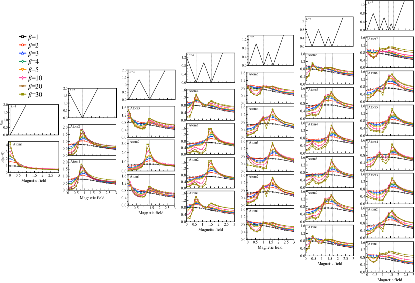
Figure 11: QMC results for spectral function at $\omega=0$ as a function of an external magnetic field for $J_{k}/t=2$, $J_{h}/t=1.8$ and for different values of inverse temperature $\beta=t/k_{B}T$ up to $L=7$. This figure is directly comparable with Fig.3 reported in Ref. [Toskovic et al., 2016] along a cut on zero bias conductance data around 330 mK.

.3 Large-N mean field for the infinite Heisenberg chain of adatoms

We consider an infinite Heisenberg chain of adatoms with periodic boundary conditions. The unit cell, $\boldsymbol{l}$, contains $n\in\left[1\cdots N_{c}\right]$ conduction electrons $\hat{c}_{\boldsymbol{l},n,\sigma}$ and a single spin degree of freedom. In this case, we can use the identity $J_{h}\boldsymbol{S}_{\boldsymbol{l}}\cdot\boldsymbol{S}_{\boldsymbol{l}+1}=-\frac{J_{h}}{4}\left(D_{\boldsymbol{l},\boldsymbol{l}+1}D^{\dagger}_{\boldsymbol{l},\boldsymbol{l}+1}+D^{\dagger}_{\boldsymbol{l},\boldsymbol{l}+1}D_{\boldsymbol{l},\boldsymbol{l}+1}\right)$ with $\boldsymbol{S}_{l}=\frac{1}{2}\boldsymbol{d}^{\dagger}_{l}\boldsymbol{\sigma}\boldsymbol{d}_{\boldsymbol{l}}$, $D_{\boldsymbol{l},\boldsymbol{l}+1}=\boldsymbol{d}^{\dagger}_{\boldsymbol{l}}\boldsymbol{d}_{\boldsymbol{l}+1}$ and constraint $\boldsymbol{d}^{\dagger}_{\boldsymbol{l}}\boldsymbol{d}_{\boldsymbol{l}}=1$ to define the large-N mean-field saddle point of Eq. (1)

$$\hat{H}_{MF}= \sum_{n,n^{\prime},k,\sigma}\hat{c}^{\dagger}_{k,n,\sigma}T(k)_{n,n^{\prime}}\hat{c}_{k,n,\sigma}-\frac{J_{h}\chi}{4}\sum_{\boldsymbol{l},\sigma}(\hat{d}^{\dagger}_{\boldsymbol{l},\sigma}\hat{d}_{{\boldsymbol{l}}+1,\sigma}+h.c.)-\frac{1}{2}g\mu_{B}h^{z}\sum_{l,\sigma}\sigma\hat{d}^{\dagger}_{\boldsymbol{l},\sigma}\hat{d}_{\boldsymbol{l},\sigma}$$

$$-\frac{J_{k}V}{4}\sum_{{\boldsymbol{l}},\sigma}\left(\hat{c}^{\dagger}_{{\boldsymbol{l}},0,\sigma}\hat{d}_{\boldsymbol{l},0,\sigma}+h.c.\right)-\lambda\sum_{{\boldsymbol{l}},\sigma}\hat{d}^{\dagger}_{{\boldsymbol{l}},\sigma}\hat{d}_{{\boldsymbol{l}},\sigma}$$

describing the hybridization of a band of spinons with the conduction electron. Here the mean field order parameters $V=\langle\hat{c}^{\dagger}_{\boldsymbol{l},0,\sigma}\hat{d}_{\boldsymbol{l},0,\sigma}\rangle$ and $\chi=\langle\hat{d}^{\dagger}_{\boldsymbol{l},\sigma}\hat{d}_{\boldsymbol{l}+1,\sigma}\rangle$ have to be determined self-consistently and the Lagrange multiplier $\lambda$ enforces the constraint on average.