A Polynomial-time Solution for Robust
Registration with Extreme Outlier Rates

Abstract

We propose a robust approach for the registration of two sets of 3D points in the presence of a large amount of outliers. Our first contribution is to reformulate the registration problem using a Truncated Least Squares (TLS) cost that makes the estimation insensitive to a large fraction of spurious point-to-point correspondences. The second contribution is a general framework to decouple rotation, translation, and scale estimation, which allows solving in cascade for the three transformations. Since each subproblem (scale, rotation, and translation estimation) is still non-convex and combinatorial in nature, out third contribution is to show that (i) TLS scale and (component-wise) translation estimation can be solved exactly and in polynomial time via an adaptive voting scheme, (ii) TLS rotation estimation can be relaxed to a semidefinite program and the relaxation is tight in practice, even in the presence of an extreme amount of outliers. We validate the proposed algorithm, named TEASER (Truncated least squares Estimation And SEmidefinite Relaxation), in standard registration benchmarks showing that the algorithm outperforms RANSAC and robust local optimization techniques, and favorably compares with Branch-and-Bound methods, while being a polynomial-time algorithm. TEASER can tolerate up to ${99\%}$ outliers and returns highly-accurate solutions.

I Introduction

Point cloud registration is a fundamental problem in robotics and computer vision and consists in finding the best transformation (rotation, translation, and potentially scale) that aligns two point clouds. It finds applications in motion estimation and 3D reconstruction [30, 7, 18, 61], object recognition and localization [21, 56, 59, 43], panorama stitching [4], and medical imaging [3, 53], to name a few.

When the ground-truth correspondences between the point clouds are known and the noise follows a zero-mean Gaussian distribution, the registration problem can be readily solved, since elegant closed-form solutions [31, 2] exist for the case of isotropic noise, and recently proposed convex relaxations [10] are empirically tight even in the presence of large anisotropic noise. In practice, however, the correspondences are either unknown, or contain a high ratio of outliers. Large outlier rates are typical of 3D keypoint detection and matching techniques [55, 49]. Therefore, it is common to use the aforementioned methods within a RANSAC scheme [23].

While RANSAC is a popular approach for several robust vision and robotics problems, its runtime grows exponentially with the outlier ratio [12] and it can perform poorly with extreme outlier rates. The capability of tolerating a large amount of outliers is of paramount importance in applications where the correspondences are unknown and when operating in the clutter (e.g., object pose estimation in the wild). Moreover, even when the correspondences are known but uncertain, it is desirable to develop registration techniques that can afford stronger performance guarantees compared to RANSAC.

This paper is motivated by the goal of designing an approach that (i) can solve registration globally (without relying on an initial guess), (ii) can tolerate extreme amounts of outliers (e.g., when ${99\%}$ of the measurements are outliers), (iii) runs in polynomial time, and (iv) provides formal performance guarantees. The related literature, reviewed in Section II, fails to simultaneously address all these aspects, and only includes techniques that are robust to moderate amounts (e.g., ${60\%}$) of outliers and lack optimality guarantees (e.g., FGR [62]), or are globally optimal but run in exponential time in the worst case, such as branch-and-bound (BnB) methods (e.g., Go-ICP [58]).

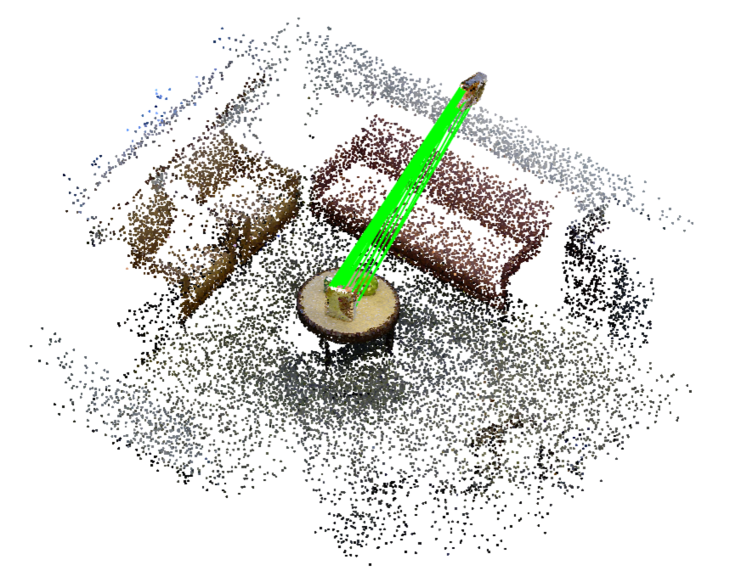
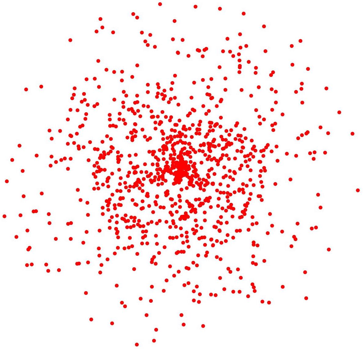(a) Cluttered scene

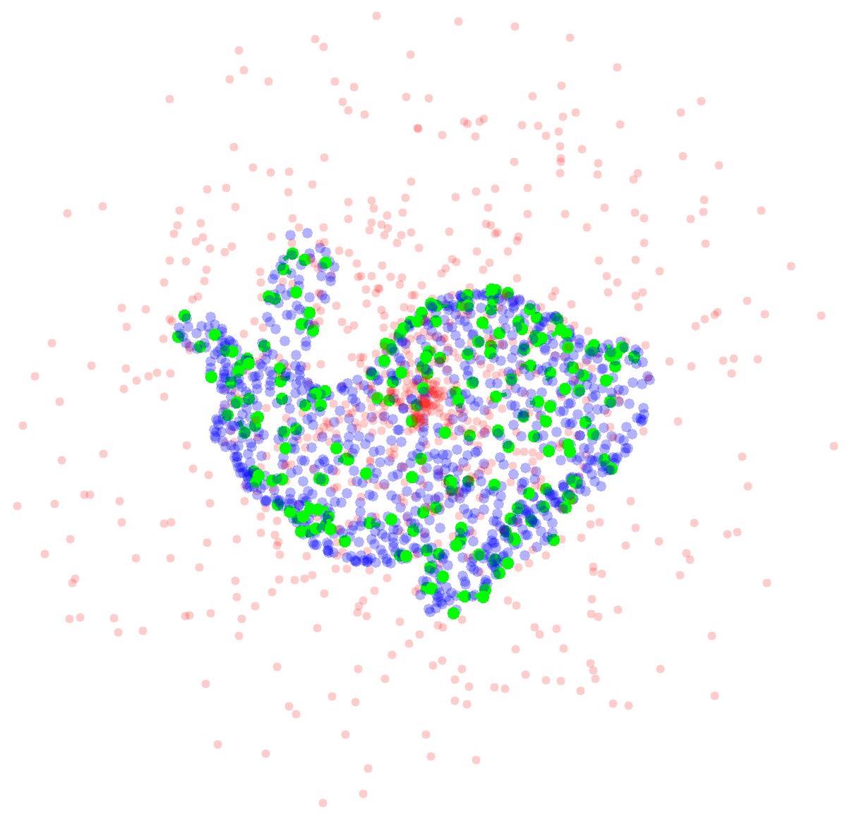(b) Registration result

Figure 1: We address 3D point cloud registration with extreme outlier rates. (a) Bunny dataset spoiled with 80% outlier correspondences: finding/localizing the bunny is challenging even for a human; (b) The proposed Truncated least squares Estimation And SEmidefinite Relaxation (TEASER) is able to find the correct inlier correspondences (green) and compute the correct registration result in polynomial time. TEASER is robust to 99% outlier correspondences.

Contribution. Our first contribution (presented in Section III) is to reformulate the registration problem using a Truncated Least Squares (TLS) cost that is insensitive to a large fraction of spurious data. We name the resulting problem the Truncated Least Squared Registration (TR) problem.

The second contribution (Section IV) is a general framework to decouple scale, rotation, and translation estimation. The idea of decoupling rotation and translation has appeared in related work, e.g., [42, 40, 12]. The novelty of our proposal is threefold: (i) we develop invariant measurements to estimate the scale ([40, 12] assume the scale is given), (ii) we make the decoupling formal within the framework of unknown-but-bounded noise [45], and (iii) we provide a general graph-theoretic framework to derive these invariant measurements.

The decoupling allows solving in cascade for scale, rotation, and translation. However, each subproblem is still combinatorial in nature. Our third contribution is to show that (i) in the scalar case TLS estimation can be solved exactly in polynomial time using an adaptive voting scheme, and this enables efficient estimation of the scale and the (component-wise) translation; (ii) we can prune a large amount of outliers by finding a maximal clique of the graph defined by the invariant measurements; (iii) we can formulate a tight semidefinite programming (SDP) relaxation to estimate the rotation, (iv) we can provide per-instance bounds on the performance of the SDP relaxation. To the best of our knowledge, this is the first polynomial-time algorithm for outlier-robust registration with computable performance guarantees.

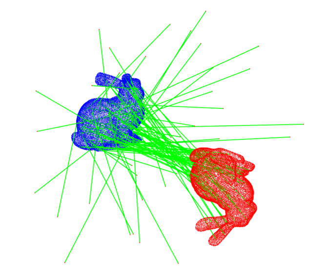
We validate the proposed algorithm, named Truncated least squares Estimation And SEmidefinite Relaxation (TEASER), in standard registration benchmarks as well as robotics datasets, showing that the algorithm outperforms RANSAC and robust local optimization techniques, and favorably compares with Branch-and-Bound methods, while being a polynomial-time algorithm. TEASER can tolerate up to ${99\%}$ outliers (Fig. 1) and returns highly-accurate solutions.

II Related Work

There are two established paradigms for the registration of 3D point clouds: Correspondence-based and Simultaneous Pose and Correspondence methods.

II-A Correspondence-based Methods

Correspondence-based methods first detect and match 3D keypoints between point clouds using local [55, 26, 49, 50] or global [21, 36] descriptors to establish putative correspondences, and then either use closed-form solutions [31, 2] in a RANSAC [23] scheme, or apply robust optimization methods [62, 12] to gain robustness against outliers. 3D keypoint matching is known to be less accurate compared to 2D counterparts like SIFT and ORB, thus causing much higher outlier rates, e.g., having 95% spurious correspondences is considered common [12]. Therefore, a robust backend that can deal with extreme outlier rates is highly desirable.

Registration without outliers. Horn [31] and Arun [2] show that optimal solutions (in the maximum likelihood sense) for scale, rotation, and translation can be computed in closed form when the points are affected by isotropic zero-mean Gaussian noise. Olsson et al. [47] propose a method based on BnB that is globally optimal and allows point-to-point, point-to-line, and point-to-plane correspondences. Recently, Briales and Gonzalez-Jimenez [10] propose a semidefinite relaxation that can deal with anisotropic Gaussian noise, and has per-instance optimality guarantees.

Robust registration. Probably the most widely used robust registration approach is based on RANSAC [23, 16], which has enabled several early applications in vision and robotics [27, 44]. Despite its efficiency in the low-noise and low-outlier regime, RANSAC exhibits slow convergence and low accuracy with large outlier rates [12], where it becomes harder to sample a “good” consensus set. Other approaches resort to M-estimation, which replaces the least squares objective function with robust costs that are less sensitive to outliers [54, 6, 38]. Zhou et al. [62] propose Fast Global Registration (FGR) that uses the Geman-McClure cost function and leverages graduated non-convexity to solve the resulting non-convex optimization. Since graduated non-convexity has to be solved in discrete steps, FGR does not guarantee global optimality [12]. Indeed, FGR tends to fail when the outlier ratio is high (>80%), as we show in Section VI. Bustos and Chin [12] propose a Guaranteed Outlier REmoval (GORE) technique, that uses geometric operations to significantly reduce the amount of outlier correspondences before passing them to the optimization backend. GORE has been shown to be robust to 95% spurious correspondences [12]. However, GORE does not estimate the scale of the registration and has exponential worst-case time complexity due to the possible usage of BnB (see Algorithm 2 in [12]).

II-B Simultaneous Pose and Correspondence Methods

Simultaneous Pose and Correspondence (SPC) methods alternate between finding the correspondences and computing the best transformation given the correspondences.

Local methods. The Iterative Closest Point (ICP) algorithm [5] is considered a milestone in point cloud registration. However, ICP is prone to converge to local minima and it only performs well given a good initial guess. Multiple variants of ICP [24, 51, 60, 41, 17, 35, 8] have proposed to use robust cost functions to improve convergence. Probabilistic interpretations have also been proposed to improve ICP convergence, for instance interpreting the registration problem as a minimization of the Kullback-Leibler divergence between two Gaussian Mixture Models [33, 46, 34, 14]. All these methods rely on iterative local search, do not provide global optimality guarantees, and typically fail without a good initial guess.

Global methods. Global SPC approaches compute a globally optimal solution without initial guesses, and are usually based on BnB, which at each iteration divides the parameter space into multiple sub-domains (branch) and computes the bounds of the objective function for each sub-domain (bound). A series of geometric techniques have been proposed to improve the bounding tightness [29, 9, 58, 15, 13] and increase the search speed [58, 39]. However, the runtime of BnB increases exponentially with the size of the point cloud and it can be made worse by the explosion of the number of local minima resulting from high outlier ratios [12]. Global SPC registration can be also formulated as a mixed-integer program [32], though the runtime remains exponential.

III Robust Registration with
Truncated Least Squares Cost

In the robust registration problem, we are given two 3D point sets ${\cal A}=\{{\bm{a}}_{i}\}_{i=1}^{N}$ and ${\cal B}=\{{\bm{b}}_{i}\}_{i=1}^{N}$, with ${\bm{a}}_{i},{\bm{b}}_{i}\in{{\mathbb{R}}^{3}}$, such that:

$${\bm{b}}_{i}=s{\bm{R}}{\bm{a}}_{i}+{\bm{t}}+{\bm{o}}_{i}+{\bm{\epsilon}}_{i}$$ (1)

where $s>0$, ${\bm{R}}\!\in\!\mathrm{SO}(3)$, and ${\bm{t}}\!\in\!{{\mathbb{R}}^{3}}$ are an unknown scale, rotation, and translation, ${\bm{\epsilon}}_{i}$ models measurement noise, and ${\bm{o}}_{i}$ is a vector of zeros for inliers, or a vector of arbitrary numbers for outliers. In words, if the $i$-th correspondence $({\bm{a}}_{i},{\bm{b}}_{i})$ is an inlier, ${\bm{b}}_{i}$ corresponds to a 3D transformation of ${\bm{a}}_{i}$ (plus noise), while if $({\bm{a}}_{i},{\bm{b}}_{i})$ is an outlier correspondence, ${\bm{b}}_{i}$ is just an arbitrary vector. $\mathrm{SO}(3)\doteq\{{\bm{R}}\in{{\mathbb{R}}^{3\times 3}}\;{:}\;{\bm{R}}^{\mathsf{T}}{\bm{R}}={\mathbf{I}}_{3},\det({\bm{R}})=+1\}$ is the set of proper rotation matrices (where ${\mathbf{I}}_{d}$ is the identity matrix of size $d$). We consider a correspondence-based setup, where we need to compute $(s,{\bm{R}},{\bm{t}})$ given putative correspondences $({\bm{a}}_{i},{\bm{b}}_{i}),i=1,\ldots,N$.

Registration without outliers. When ${\bm{\epsilon}}_{i}$ is a zero-mean Gaussian noise with isotropic covariance $\sigma_{i}^{2}{\mathbf{I}}_{3}$, and all the correspondences are correct (i.e., ${\bm{o}}_{i}=\bm{0},\forall i$), the Maximum Likelihood estimator of $(s,{\bm{R}},{\bm{t}})$ can be computed in closed form by decoupling the estimation of the scale, translation, and rotation, using Horn’s [31] or Arun’s method [2].

Robust registration. In practice, a large fraction of the correspondences are outliers, due to incorrect keypoint matching. Despite the elegance of the closed-form solutions [31, 2], they are not robust to outliers, and a single “bad” outlier can compromise the correctness of the resulting estimate. Hence, we propose a truncated least squares registration formulation that can tolerate extreme amounts of spurious data.

Truncated Least Squares Registration. We depart from the Gaussian noise model and assume the noise is unknown but bounded [45]. Formally, we assume the noise ${\bm{\epsilon}}_{i}$ in (1) is such that $\|{\bm{\epsilon}}_{i}\|\leq\beta_{i}$, where $\beta_{i}$ is a given bound.

Then we adopt the following Truncated Least Squares Registration (TR) formulation :

$$\min_{\begin{subarray}{c}s>0,{\bm{t}}\in{{\mathbb{R}}^{3}},{\bm{R}}\in\mathrm{SO}(3)\end{subarray}}\sum_{i=1}^{N}\min\left(\frac{1}{\beta_{i}^{2}}\left\|{\bm{b}}_{i}-s{\bm{R}}{\bm{a}}_{i}-{\bm{t}}\right\|^{2}\;,\;\bar{c}^{2}\right)$$ (2)

which computes a least squares solution of measurements with small residual ($\frac{1}{\beta_{i}^{2}}\left\|{\bm{b}}_{i}-s{\bm{R}}{\bm{a}}_{i}-{\bm{t}}\right\|^{2}\leq\bar{c}^{2}$), while discarding measurements with large residuals (when $\frac{1}{\beta_{i}^{2}}\left\|{\bm{b}}_{i}-s{\bm{R}}{\bm{a}}_{i}-{\bm{t}}\right\|^{2}>\bar{c}^{2}$ the $i$-th summand becomes constant and does not influence the optimization). The constant $\bar{c}^{2}$ is typically chosen to be $1$, while one may use a different $\bar{c}^{2}$ to be stricter or more lenient towards potential outliers.

IV Decoupling Scale, Rotation,
and Translation Estimation

We propose a polynomial-time algorithm that decouples the estimation of scale, translation, and rotation in problem (2). The key insight is that we can reformulate the measurements (1) to obtain quantities that are invariant to a subset of the transformations (scaling, rotation, translation).

IV-A Translation Invariant Measurements (TIM)

While the absolute positions of the points in ${\cal B}$ depend on the translation ${\bm{t}}$, the relative positions are invariant to ${\bm{t}}$. Mathematically, given two points ${\bm{b}}_{i}$ and ${\bm{b}}_{j}$ from (1), the relative position of these two points is:

$${\bm{b}}_{j}-{\bm{b}}_{i}=s{\bm{R}}({\bm{a}}_{j}-{\bm{a}}_{i})+({\bm{o}}_{j}-{\bm{o}}_{i})+({\bm{\epsilon}}_{j}-{\bm{\epsilon}}_{i})$$ (3)

where the translation ${\bm{t}}$ cancels out in the subtraction. Therefore, we can obtain a Translation Invariant Measurement (TIM) by computing $\bar{{\bm{a}}}_{ij}\doteq{\bm{a}}_{j}-{\bm{a}}_{i}$ and $\bar{{\bm{b}}}_{ij}\doteq{\bm{b}}_{j}-{\bm{b}}_{i}$, and the TIM satisfies the following generative model:

$$\bar{{\bm{b}}}_{ij}=s{\bm{R}}\bar{{\bm{a}}}_{ij}+{\bm{o}}_{ij}+{\bm{\epsilon}}_{ij}$$ (TIM)

where ${\bm{o}}_{ij}\doteq{\bm{o}}_{j}-{\bm{o}}_{i}$ is zero if both the $i$-th and the $j$-th measurements are inliers (or it is an arbitrary vector otherwise), while ${\bm{\epsilon}}_{ij}\doteq{\bm{\epsilon}}_{j}-{\bm{\epsilon}}_{i}$ is the measurement noise. It is easy to see that if $\|{\bm{\epsilon}}_{i}\|\leq\beta_{i}$ and $\|{\bm{\epsilon}}_{j}\|\leq\beta_{j}$ then $\|{\bm{\epsilon}}_{ij}\|\leq\beta_{i}+\beta_{j}\doteq\beta_{ij}$.

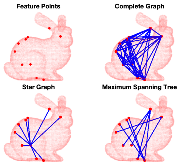
The advantage of the TIMs in eq. (TIM) is that their generative model only depends on two unknowns, $s$ and ${\bm{R}}$. The number of TIMs is upper-bounded by $\left(\begin{subarray}{c}N\\ 2\end{subarray}\right)=N(N-1)/2$, where pairwise relative measurements between all pairs of points are computed. For computational reasons, one might want to downsample the TIMs. Theorem 1 below provides a graph-theoretic way to create the TIMs.

Theorem 1 (Translation Invariant Measurements).

Define the vectors ${\bm{a}}\in{{\mathbb{R}}^{3N}}$ (resp. ${\bm{b}}\in{{\mathbb{R}}^{3N}}$), obtained by concatenating all vectors ${\bm{a}}_{i}$ (resp. ${\bm{b}}_{i}$) in a single column vector. Moreover, define an arbitrary graph ${\cal G}$ with nodes $\{1,\ldots,N\}$ and an arbitrary set of edges ${\cal E}$. Then, the vectors $\bar{{\bm{a}}}=({\bm{A}}\otimes{\mathbf{I}}_{3}){\bm{a}}$ and $\bar{{\bm{b}}}=({\bm{A}}\otimes{\mathbf{I}}_{3}){\bm{b}}$ are TIMs, where ${\bm{A}}\in{{\mathbb{R}}^{|{\cal E}|\times N}}$ is the incidence matrix of ${\cal G}$, and $\otimes$ is the Kronecker product.

A proof of the theorem is given in the Supplementary Material. Three potential graph topologies for generating TIMs are illustrated in Fig. 2.

Figure 2: Graph topologies for generating TIMs in the Bunny dataset.

IV-B Translation and Rotation Invariant Measurements (TRIM)

While the relative locations of pairs of points (TIMs) still depends on the rotation ${\bm{R}}$, their distances are invariant to both ${\bm{R}}$ and ${\bm{t}}$. Therefore, to build rotation invariant measurements, we compute the norm of each TIM vector:

$$\|\bar{{\bm{b}}}_{ij}\|=\|s{\bm{R}}\bar{{\bm{a}}}_{ij}+{\bm{o}}_{ij}+{\bm{\epsilon}}_{ij}\|$$ (4)

We now note that for the inliers (${\bm{o}}_{ij}=\bm{0}$) it holds (using $\|{\bm{\epsilon}}_{ij}\|\leq\beta_{ij}$ and the triangle inequality):

$$\|s{\bm{R}}\bar{{\bm{a}}}_{ij}\|-\beta_{ij}\leq\|s{\bm{R}}\bar{{\bm{a}}}_{ij}+{\bm{\epsilon}}_{ij}\|\leq\|s{\bm{R}}\bar{{\bm{a}}}_{ij}\|+\beta_{ij}$$ (5)

hence we can write (4) equivalently as:

$$\|\bar{{\bm{b}}}_{ij}\|=\|s{\bm{R}}\bar{{\bm{a}}}_{ij}\|+\tilde{o}_{ij}+\tilde{{\epsilon}}_{ij}$$ (6)

with $|\tilde{{\epsilon}}_{ij}|\leq\beta_{ij}$, and $\tilde{o}_{ij}=0$ if both $i$ and $j$ are inliers or is an arbitrary scalar otherwise. Recalling that the norm is rotation invariant and that $s>0$, and dividing both members of (6) by $\|\bar{{\bm{a}}}_{ij}\|$, we obtain new measurements $s_{ij}\doteq\frac{\|\bar{{\bm{b}}}_{ij}\|}{\|\bar{{\bm{a}}}_{ij}\|}$:

$$s_{ij}=s+o^{s}_{ij}+{\epsilon}^{s}_{ij}$$ (TRIM)

where ${\epsilon}^{s}_{ij}\doteq\frac{\tilde{{\epsilon}}_{ij}}{\|\bar{{\bm{a}}}_{ij}\|}$, and $o^{s}_{ij}\doteq\frac{\tilde{o}_{ij}}{\|\bar{{\bm{a}}}_{ij}\|}$. It is easy to see that $|{\epsilon}^{s}_{ij}|\leq\beta_{ij}/\|\bar{{\bm{a}}}_{ij}\|$ since $|\tilde{{\epsilon}}_{ij}|\leq\beta_{ij}$. We define $\alpha_{ij}\doteq\beta_{ij}/\|\bar{{\bm{a}}}_{ij}\|$.

Eq. (TRIM) describes a translation and rotation invariant measurement (TRIM) whose generative model is only function of the unknown scale $s$. A summary table of the invariant measurements and a remark on the novelty of creating TIMs and TRIMs is presented in the Supplementary Material .

IV-C Our Registration Algorithm: Truncated least squares Estimation And SEmidefinite Relaxation (TEASER)

We propose a decoupled approach to solve in cascade for the scale, the rotation, and the translation in (2). The approach, named Truncated least squares Estimation And SEmidefinite Relaxation (TEASER), works as follows:

1. we use the TRIMs to estimate the scale $\hat{s}$

2. we use $\hat{s}$ and the TIMs to estimate the rotation $\hat{\bm{R}}$

3. we use $\hat{s}$ and $\hat{\bm{R}}$ to estimate the translation $\hat{\bm{t}}$ from the original TLS problem (2).

The pseudocode is also summarized in Algorithm 1.

1 Input:  points $({\bm{a}}_{i},{\bm{b}}_{i})$ and bounds $\beta_{i}$ ($i=1,\ldots,N$), threshold $\bar{c}^{2}$ (default: $\bar{c}^{2}=1$), graph edges ${\cal E}$ (default: ${\cal E}$ describes the complete graph);

2 Output:   $s,{\bm{R}},{\bm{t}}$;

3 % Compute TIM and TRIM

4 $\bar{{\bm{b}}}_{ij}={\bm{b}}_{j}-{\bm{b}}_{i}\;,\;\bar{{\bm{a}}}_{ij}={\bm{a}}_{j}-{\bm{a}}_{i}\;,\;\beta_{ij}=\beta_{i}+\beta_{j}\;\;\forall(i,j)\in{\cal E}$

5 $s_{ij}=\frac{\|\bar{{\bm{b}}}_{ij}\|}{\|\bar{{\bm{a}}}_{ij}\|}\;,\;\alpha_{ij}=\frac{\beta_{ij}}{\|\bar{{\bm{a}}}_{ij}\|}\;\;\forall(i,j)\in{\cal E}$

6 % Decoupled estimation of $s,{\bm{R}},{\bm{t}}$

7 $\hat{s}={\tt estimate\_s}(\{s_{ij},\alpha_{ij}:\forall(i,j)\in{\cal E}\},\bar{c}^{2})$

8 $\hat{{\bm{R}}}={\tt estimate\_R}(\{\bar{{\bm{a}}}_{ij},\bar{{\bm{b}}}_{ij},\beta_{ij}:\forall(i,j)\in{\cal E}\},\bar{c}^{2},\hat{s})$

9 $\hat{{\bm{t}}}={\tt estimate\_t}(\{{\bm{a}}_{i},{\bm{b}}_{i},\beta_{i}:i=1\ldots,N\},\bar{c}^{2},\hat{s},\hat{{\bm{R}}})$

return: $\hat{s},\hat{{\bm{R}}},\hat{{\bm{t}}}$

Algorithm 1 Truncated least squares Estimation And SEmidefinite Relaxation (TEASER).

The following section describes how to implement the functions in lines 1-1 of Algorithm 1. In particular, we show how to obtain global and robust estimates of scale (${\tt estimate\_s}$) in Section V-A, rotation (${\tt estimate\_R}$) in Section V-B, and translation (${\tt estimate\_t}$) in Section V-C.

V Solving the Registration Subproblems

V-A Robust Scale Estimation

The generative model (TRIM) describes linear measurements $s_{ij}$ of the unknown scale $s$, affected by bounded noise $|{\epsilon}^{s}_{ij}|\leq\alpha_{ij}$ including potential outliers (when $o^{s}_{ij}\neq 0$). Again, we estimate the scale given the measurements $s_{ij}$ and the bounds $\alpha_{ij}$ using a TLS estimator:

$$\hat{s}=\operatorname*{arg\,min}_{s}\sum_{k=1}^{K}\min\left(\frac{(s-s_{k})^{2}}{\alpha^{2}_{k}}\;,\;\bar{c}^{2}\right)$$ (7)

where for simplicity we numbered the measurements from $1$ to $K=|{\cal E}|$ and adopted the notation $s_{k}$ instead of $s_{ij}$.

The following theorem shows that one can solve (7) in polynomial time by a simple enumeration.

Theorem 2 (Optimal TLS Scale Estimation).

For a given $s\in{{\mathbb{R}}}$, define the consensus set of $s$ as ${\cal C}(s)=\{k\;{:}\;\frac{(s-s_{k})^{2}}{\alpha^{2}_{k}}\leq\bar{c}^{2}\}$. Then, for any $s\in{{\mathbb{R}}}$, there are at most $2K-1$ different non-empty consensus sets. If we name these sets ${\cal C}_{1},\ldots,{\cal C}_{2K-1}$, then the solution of (7) can be computed by enumeration as:

$$\hat{s}=\operatorname*{arg\,min}\left\{f_{s}(\hat{s}_{i}):\hat{s}_{i}=\left(\sum_{k\in{\cal C}_{i}}\frac{1}{\alpha_{k}^{2}}\right)^{-1}\sum_{k\in{\cal C}_{i}}\frac{s_{k}}{\alpha_{k}^{2}},\forall i\right\}$$ (8)

where $f_{s}(\cdot)$ is the objective function of (7).

Theorem 2, whose proof is given in the Supplementary Material, is based on the insight that the consensus set can only change at the boundaries of the intervals $[s_{k}-\alpha_{k}\bar{c},s_{k}+\alpha_{k}\bar{c}]$ (Fig. 3(a)) and there are at most $2K$ such boundaries. The theorem also suggests a straightforward adaptive voting algorithm to solve (7), with pseudocode given in Algorithm 2. The algorithm first builds the boundaries of the intervals shown in Fig. 3(a) (line 2). Then, for each interval, it evaluates the consensus set (line 2, see also Fig. 3(b)). Since the consensus set does not change within an interval, we compute it at the interval centers (line 2, see also Fig. 3(b)). Finally, the cost of each consensus set is computed and the smallest cost is returned as optimal solution (line 2).

Figure 3: (a) confidence interval for each measurement $s_{k}$ (every $s$ in the $k$-th interval satisfies $\frac{\|s-s_{k}\|^{2}}{\alpha_{k}^{2}}\leq\bar{c}^{2}$; (b) cardinality of the consensus set for every $s$ and middle-points $m_{j}$ for each interval with constant consensus set.

1 Input:  $s_{k},\alpha_{k},\bar{c}$;

2 Output:   $\hat{s}$, scale estimate solving (7);

3 % Define boundaries and sort

4 ${\bm{v}}=\text{sort}([s_{1}-\alpha_{1}\bar{c},s_{1}+\alpha_{1}\bar{c},\ldots,s_{K}-\alpha_{K}\bar{c},s_{K}+\alpha_{K}\bar{c}])$

5 % Compute middle points

6$m_{i}=\frac{{\bm{v}}_{2i-1}+{\bm{v}}_{2i}}{2}$ for $i=1,\ldots,2K-1$

7% Voting

8for $i=1,\ldots,2K-1$ do

9       ${\cal S}_{i}=\emptyset$

10       for $k=1,\ldots,K$ do

11             if $m_{i}\in[s_{k}-\alpha_{k}\bar{c},s_{k}+\alpha_{k}\bar{c}]$ then

12                   ${\cal S}_{i}={\cal S}_{i}\cup\{k\}$ % add to consensus set

13                  

14             end if

15            

16       end for

17      

18 end for

19% Enumerate consensus sets and return best

return: $\!\operatorname*{arg\,min}\left\{f_{s}(\hat{s}_{i}):\hat{s}_{i}=\left(\displaystyle\sum_{k\in{\cal C}_{i}}\frac{1}{\alpha_{k}^{2}}\right)^{-1}\displaystyle\sum_{k\in{\cal C}_{i}}\frac{s_{k}}{\alpha_{k}^{2}},\forall i\right\}\!\!$

Algorithm 2 Adaptive Voting.

The interested reader can find a discussion on the relation between TLS and consensus maximization (a popular approach for outlier detection [52, 40]) in the Supplementary Material.

Maximal clique inlier selection (MCIS). The graph theoretic interpretation of Theorem 1 offers further opportunities to prune outliers. Considering the TRIMs as edges in the graph ${\cal G}({\cal V},{\cal E})$ (where the vertices ${\cal V}$ are the 3D points and the edge set ${\cal E}$ induces the TIMs and TRIMs per Theorem 1), we can use the scale estimate $\hat{s}$ from Algorithm 2 to prune edges $(i,j)$ in the graph whose associated TRIM $s_{ij}$ is such that $\frac{(s_{ij}-\hat{s})^{2}}{\alpha_{ij}^{2}}\!\!>\!\!\bar{c}^{2}$. This allows us to obtain a pruned graph ${\cal G}^{\prime}({\cal V},{\cal E}^{\prime})$, with ${\cal E}^{\prime}\subseteq{\cal E}$, where gross outliers are discarded. The following result ensures that inliers form a clique in the graph ${\cal G}^{\prime}({\cal V},{\cal E}^{\prime})$ enabling an even more substantial rejection of outliers.

Theorem 3 (Maximal Clique Inlier Selection).

Edges corresponding to inlier TIMs form a clique in ${\cal E}^{\prime}$, and there is at least one maximal clique in ${\cal E}^{\prime}$ that contains all the inliers.

A proof of Theorem 3 is presented in the Supplementary Material. Theorem 3 allows us to prune outliers by finding the maximal cliques of ${\cal G}^{\prime}({\cal V},{\cal E}^{\prime})$. Although finding the maximal cliques of a graph takes exponential time in general, there exist efficient approximation algorithms based on heuristics [11, 48, 57] . In addition, under high outlier rates, the graph ${\cal G}^{\prime}({\cal V},{\cal E}^{\prime})$ is sparse and the maximal clique problem can be solved quickly in practice [22]. In this paper, we choose the maximal clique with largest cardinality, i.e., the maximum clique , as the inlier set to pass to rotation estimation. Section VI-A shows that this method drastically reduces the number of outliers.

In summary, the function ${\tt estimate\_s}$ in Algorithm 1 first calls Algorithm 2, then computes the maximum clique in the resulting graph to reject all measurements outside the clique.

What if the scale is known? In some registration problems, the scale is known, e.g., the scale of the two point clouds is the same. In such a case, we can skip Algorithm 2 and set $\hat{s}$ to be the known scale. Moreover, we can still use the MCIS method to largely reduce the number of outliers.

V-B Robust Rotation Estimation

The generative model (TIM) describes measurements $\bar{{\bm{b}}}_{ij}$ affected by bounded noise $\|{\bm{\epsilon}}_{ij}\|\leq\beta_{ij}$ including potential outliers (when ${\bm{o}}_{ij}\neq\bm{0}$). Again, we estimate ${\bm{R}}$ from the estimated scale $\hat{s}$, the measurements $\bar{{\bm{b}}}_{ij}$ and the bounds $\beta_{ij}$ using a TLS estimator:

$$\hat{{\bm{R}}}=\operatorname*{arg\,min}_{{\bm{R}}\in\mathrm{O}(3)}\sum_{k=1}^{K}\min\left(\frac{\|\bar{{\bm{b}}}_{k}-\hat{s}{\bm{R}}\bar{{\bm{a}}}_{k}\|^{2}}{\beta^{2}_{k}}\;,\;\bar{c}^{2}\right)$$ (9)

where for simplicity we numbered the measurements from $1$ to $K=|{\cal E}|$ and adopted the notation $\bar{{\bm{a}}}_{k},\bar{{\bm{b}}}_{k}$ instead of $\bar{{\bm{a}}}_{ij},\bar{{\bm{b}}}_{ij}$. We have also relaxed ${\bm{R}}\in\mathrm{SO}(3)$ to ${\bm{R}}\in\mathrm{O}(3)$, where $\mathrm{O}(3)\doteq\{{\bm{R}}\in{{\mathbb{R}}^{3\times 3}}\;{:}\;{\bm{R}}^{\mathsf{T}}{\bm{R}}={\mathbf{I}}_{3}\}$ is the Orthogonal Group, which includes proper rotations and reflections. For simplicity of notation, in the following we drop $\hat{s}$ and assume that $\bar{{\bm{a}}}_{1},\ldots,\bar{{\bm{a}}}_{K}$ have been corrected by the scale ($\bar{{\bm{a}}}_{k}\leftarrow\hat{s}\bar{{\bm{a}}}_{k}$).

A fundamental contribution of this paper is to develop a tight convex relaxation for (9). The relaxation is tight even in presence of a large number (90%) of outliers and provides per-instance suboptimality guarantees. Before presenting the relaxation, we introduce a binary formulation that is instrumental to develop the proposed relaxation.

Binary formulation and Binary cloning. The first insight behind our convex relaxation is the fact that we can write the TLS cost (9) in additive form using auxiliary binary variables (a property recently leveraged in a different context by [38]):

$$\min_{\begin{subarray}{c}{\bm{R}}\in\mathrm{O}(3),\\ \theta_{k}\in\{-1,+1\},\forall k\end{subarray}}\sum_{k=1}^{K}\frac{(1+\theta_{k})}{2}\frac{\|\bar{{\bm{b}}}_{k}-{\bm{R}}\bar{{\bm{a}}}_{k}\|^{2}}{\beta^{2}_{k}}+\frac{(1-\theta_{k})}{2}\bar{c}^{2}$$ (10)

The equivalence can be easily understood from the fact that $\min(x,y)=\min_{\theta\in\{-1,+1\}}\frac{(1+\theta)}{2}x+\frac{(1-\theta)}{2}y$.

We conveniently rewrite (10) by replacing the binary variables with suitable (orthogonal) matrices.

Proposition 4 (Binary cloning).

Problem (10) is equivalent to the following optimization problem

$$\min_{\begin{subarray}{c}{\bm{R}},{\bm{R}}_{k},\forall k\end{subarray}}\!\! \!\!\sum_{k=1}^{K}\frac{\|\bar{{\bm{b}}}_{k}-{\bm{R}}\bar{{\bm{a}}}_{k}+{\bm{R}}^{\mathsf{T}}{\bm{R}}_{k}\bar{{\bm{b}}}_{k}-{\bm{R}}_{k}\bar{{\bm{a}}}_{k}\|^{2}}{4\beta^{2}_{k}}+\frac{(1-{\bm{e}}_{1}^{\mathsf{T}}{\bm{R}}^{\mathsf{T}}{\bm{R}}_{k}{\bm{e}}_{1})}{2}\bar{c}^{2}$$

subject to $${\bm{R}}^{\mathsf{T}}{\bm{R}}={\mathbf{I}}_{3},\;\;{\bm{R}}_{k}^{\mathsf{T}}{\bm{R}}_{k}={\mathbf{I}}_{3},$$ (11)

$${\bm{R}}^{\mathsf{T}}{\bm{R}}_{k}\in\{-{\mathbf{I}},+{\mathbf{I}}\},\;k=1,\ldots,K$$

where we introduced a matrix ${\bm{R}}_{k}\in{{\mathbb{R}}^{3\times 3}}$ for each $k=1,\ldots,K$, and defined the vector ${\bm{e}}_{1}\doteq[1\;0\;0]^{\mathsf{T}}$.

A formal proof of Proposition 4 is given in the Supplementary Material. We name the re-parametrization in Proposition 4 binary cloning, since we now have $K$ clones of ${\bm{R}}$ (namely ${\bm{R}}_{k}=\theta_{k}{\bm{R}}\in\{{\bm{R}},-{\bm{R}}\}$, $k=1,\ldots,K$) that are in charge of rejecting outliers: when ${\bm{R}}_{k}={\bm{R}}$ the $k$-th term in the objective becomes $\frac{\|\bar{{\bm{b}}}_{k}-{\bm{R}}\bar{{\bm{a}}}_{k}\|^{2}}{\beta^{2}_{k}}$ (i.e., $k$ is treated as an inlier, similarly to choosing $\theta_{k}=+1$), while when ${\bm{R}}_{k}=-{\bm{R}}$ the $k$-th term is equal to $\bar{c}^{2}$ (i.e., $k$ is treated as an outlier, similarly to choosing $\theta_{k}=-1$). This reparametrization enables our relaxation.

Convex relaxation. The proposed relaxation is presented in Proposition 5. The main goal of this paragraph is to provide the intuition behind our relaxation, while the interested reader can find a formal derivation in the Supplementary Material.

Let us define a $3\times 3(K+2)$ matrix ${\bm{X}}=[{\mathbf{I}}_{3}\;{\bm{R}}\;{\bm{R}}_{1}\;\ldots\;{\bm{R}}_{K}]$, stacking all unknown variables in (11). We observe that the matrix ${\bm{Z}}\doteq{\bm{X}}^{\mathsf{T}}{\bm{X}}$ contains all linear and quadratic terms in ${\bm{R}}$ and ${\bm{R}}_{k}$:

$${\bm{Z}}\doteq{\bm{X}}^{\mathsf{T}}{\bm{X}}=\begin{array}[]{ccccccc}\overbrace{}^{I}\hskip 2.84526pt\overbrace{}^{R}\hskip 2.84526pt\overbrace{}^{R_{1}}\hskip 14.22636pt\ldots\hskip 14.22636pt\overbrace{}^{R_{K}}\\ \left[\begin{array}[]{ccccccc}{\mathbf{I}}_{3}&{\bm{R}}&{\bm{R}}_{1}&\ldots&{\bm{R}}_{K}\\ \star&{\mathbf{I}}_{3}&{\bm{R}}^{\mathsf{T}}{\bm{R}}_{1}&\ldots&{\bm{R}}^{\mathsf{T}}{\bm{R}}_{K}\\ \star&\star&{\mathbf{I}}_{3}&\ldots&{\bm{R}}_{1}^{\mathsf{T}}{\bm{R}}_{K}\\ \star&\vdots&\vdots&\ddots&\vdots\\ \star&\star&\star&\ldots&{\mathbf{I}}_{3}\end{array}\right]\end{array}$$ (19)

Now it is easy to see that the cost function in (11) can be rewritten as a function of ${\bm{Z}}$, by noting that ${\bm{R}},{\bm{R}}^{\mathsf{T}}{\bm{R}}_{k},{\bm{R}}_{k}$ (appearing in the cost) are entries of ${\bm{Z}}$, see (19). The constraints in (11) can be similarly written as a function of ${\bm{Z}}$. For instance, the constraints ${\bm{R}}^{\mathsf{T}}{\bm{R}}={\mathbf{I}}_{3}$ and ${\bm{R}}_{k}^{\mathsf{T}}{\bm{R}}_{k}={\mathbf{I}}_{3}$ simply enforce that the block diagonal entries of ${\bm{Z}}$ are identity matrices. Similarly, ${\bm{R}}^{\mathsf{T}}{\bm{R}}_{k}\in\{-{\mathbf{I}},+{\mathbf{I}}\}$ can be rewritten as a (non-convex) constraint involving off-diagonal entries of ${\bm{Z}}$. Finally, the fact that ${\bm{Z}}\doteq{\bm{X}}^{\mathsf{T}}{\bm{X}}$ implies ${\bm{Z}}$ is positive semidefinite and has rank $3$ (number of rows in ${\bm{X}}$, see (19)).

According to the discussion so far, we can reparametrize problem (11) using ${\bm{Z}}$, and we can then develop a convex relaxation by relaxing all the resulting non-convex constraints. This is formalized in the following proposition.

Proposition 5 (TLS Rotation Estimation: Convex Relaxation).

The following convex program is a relaxation of (11):

$$\min_{\begin{subarray}{c}{\bm{Z}}\succeq 0\end{subarray}} \mathrm{tr}\left(\bar{{\bm{Q}}}{\bm{Z}}\right)$$ (20)

subject to $$[{\bm{Z}}]_{RR}={\mathbf{I}}_{3},\;\;\;[{\bm{Z}}]_{R_{k}R_{k}}={\mathbf{I}}_{3},\;\;\;[{\bm{Z}}]_{II}={\mathbf{I}}_{3},$$

$$[{\bm{Z}}]_{RR_{k}}=({\bm{e}}_{1}^{\mathsf{T}}[{\bm{Z}}]_{RR_{k}}{\bm{e}}_{1}){\mathbf{I}}_{3},\;\;\forall k$$

$$\|[{\bm{Z}}]_{IR}\pm[{\bm{Z}}]_{IR_{k}}\|\leq 1\pm({\bm{e}}_{1}^{\mathsf{T}}[{\bm{Z}}]_{RR_{k}}{\bm{e}}_{1}),\;\;\forall k$$

$$\|[{\bm{Z}}]_{IR_{k}}\pm[{\bm{Z}}]_{IR_{k^{\prime}}}\|\leq 1\pm({\bm{e}}_{1}^{\mathsf{T}}[{\bm{Z}}]_{R_{k}R_{k^{\prime}}}{\bm{e}}_{1}),\;\;\forall k,k^{\prime}$$

where $\bar{\bm{Q}}$ is a known $3(K+2)\times 3(K+2)$ symmetric matrix (expression given in the supplementary), and $[{\bm{Z}}]_{RR_{k}}$ denotes a $3\times 3$ block of ${\bm{Z}}$ whose row indices correspond to the location of ${\bm{R}}$ in ${\bm{X}}$ (cf. with indices at the top of the matrix in eq. (19)) and column indices correspond to the location of ${\bm{R}}_{k}$ in ${\bm{X}}$ (similarly, for $[{\bm{Z}}]_{RR}$, $[{\bm{Z}}]_{R_{k}R_{k}}$, $[{\bm{Z}}]_{II}$, etc.).

The convex program (20) can be solved in polynomial time using off-the-shelf convex solvers, such as cvx [25]. It is a relaxation, in the sense that the set of feasible solutions of (20) includes the set of feasible solutions of (11). Moreover, it enjoys the typical per-instance guarantees of convex relaxations.

Proposition 6 (Guarantees for TLS Rotation Estimation).

Let ${\bm{Z}}^{\star}$ be the optimal solution of the relaxation (20). If ${\bm{Z}}^{\star}$ has rank 3, then it can be factored as ${\bm{Z}}^{\star}=({\bm{X}}^{\star})^{\mathsf{T}}({\bm{X}}^{\star})$, where ${\bm{X}}^{\star}\!\doteq\![{\mathbf{I}}_{3},{{\bm{R}}}^{\star},{{\bm{R}}}^{\star}_{1},\makebox[6.99997pt][c]{\!.\,.},{{\bm{R}}}^{\star}_{K}]$ is the first block row of ${\bm{Z}}^{\star}$. Moreover, ${{\bm{R}}}^{\star},{{\bm{R}}}^{\star}_{1},\makebox[6.99997pt][c]{\!.\,.},{{\bm{R}}}^{\star}_{K}$ is an optimal solution for (11).

Empirically, we found that our relaxation is tight (i.e., numerically produces a rank-3 solution) even when 90% of the TIMs are outliers. Even when the relaxation is not tight, one can still project ${\bm{Z}}^{\star}$ to a feasible solution of (11) and obtain an upper-bound on how suboptimal the resulting solution is.

In summary, the function ${\tt estimate\_R}$ in Algorithm 1 solves the convex program (20) (e.g., using cvx) to obtain a matrix ${\bm{Z}}^{\star}$ and extracts the rotation estimate $\hat{{\bm{R}}}$ from ${\bm{Z}}^{\star}$. In particular, $\hat{{\bm{R}}}=[{\bm{Z}}^{\star}]_{IR}$ if ${\bm{Z}}^{\star}$ has rank 3 (Proposition 6), or $\hat{{\bm{R}}}$ is computed as the projection of $[{\bm{Z}}^{\star}]_{IR}$ to $\mathrm{O}(3)$ otherwise.

V-C Robust Translation Estimation

Since we already presented a polynomial-time solution for scalar TLS in Section V-A, we propose to solve for the translation component-wise, i.e., we compute the entries $t_{1},t_{2},t_{3}$ of ${\bm{t}}$ independently (see the Supplementary Material for details):

$$\min_{\begin{subarray}{c}t_{j}\end{subarray}}\sum_{i=1}^{N}\min\left(\frac{1}{\beta_{i}^{2}}\left|[{\bm{b}}_{i}-\hat{s}\hat{{\bm{R}}}{\bm{a}}_{i}]_{j}-t_{j}\right|^{2}\!\!,\bar{c}^{2}\right),\;\;j=1,2,3$$ (21)

where $[\cdot]_{j}$ denotes the $j$-th entry of a vector.

In summary, the function ${\tt estimate\_t}$ in Algorithm 1 calls Algorithm 2 three times (one for each entry of ${\bm{t}}$) and returns the translation estimate $\hat{{\bm{t}}}=[t_{1}\;t_{2}\;t_{3}]$.

VI Experiments and Applications

The goal of this section is to (i) test the performance of our scale, rotation, translation solvers and the MCIS pruning (Section VI-A), (ii) evaluate TEASER against related techniques in benchmarking datasets (Section VI-B), (iii) evaluate TEASER with extreme outliers rates (Section VI-C), and (iv) show an application of TEASER for object localization in an RGB-D robotics dataset (Section VI-D). In all tests we set $\bar{c}^{2}=1$.

Implementation details. We implemented TEASER in matlab and used cvx to solve the convex relaxation (20). Moreover, we used the algorithm in [22] to find all the maximal cliques in the pruned TIM graph (see Theorem 3).

VI-A Testing TEASER’s Subproblems

Testing setup. We use the Bunny  point cloud from the Stanford 3D Scanning Repository [20] and resize it to be within the $[0,1]^{3}$ cube. The Bunny is first downsampled to $N=50$ points, and then a random transformation $(s,{\bm{R}},{\bm{t}})$ (with $1\leq s\leq 5$ and $\|{\bm{t}}\|\leq 1$) is applied according to eq. (1). To generate the bounded noise ${\bm{\epsilon}}_{i}$, we sample ${\bm{\epsilon}}_{i}\sim{\cal N}(\bm{0},\sigma^{2}{\bm{I}})$, until the resulting vector satisfies $\|{\bm{\epsilon}}_{i}\|\leq\beta_{i}=\beta$. We set $\sigma=0.01$ and $\beta=0.0554$ such that $\mathbb{P}\left(\|{\bm{\epsilon}}_{i}\|^{2}/\sigma^{2}>\beta^{2}\right)\leq 10^{-6}$ (this bound stems from the fact that for Gaussian ${\bm{\epsilon}}_{i}$, $\|{\bm{\epsilon}}_{i}\|^{2}$ follows a Chi-square distribution with 3 degrees of freedom). To generate outliers, we replace a fraction of ${\bm{b}}_{i}$ with vectors uniformly sampled inside the sphere of radius 5. We test increasing outlier ratios $\{0,0.2,0.4,0.6,0.7,0.8,0.9\}$. All statistics are computed over 40 Monte Carlo runs.

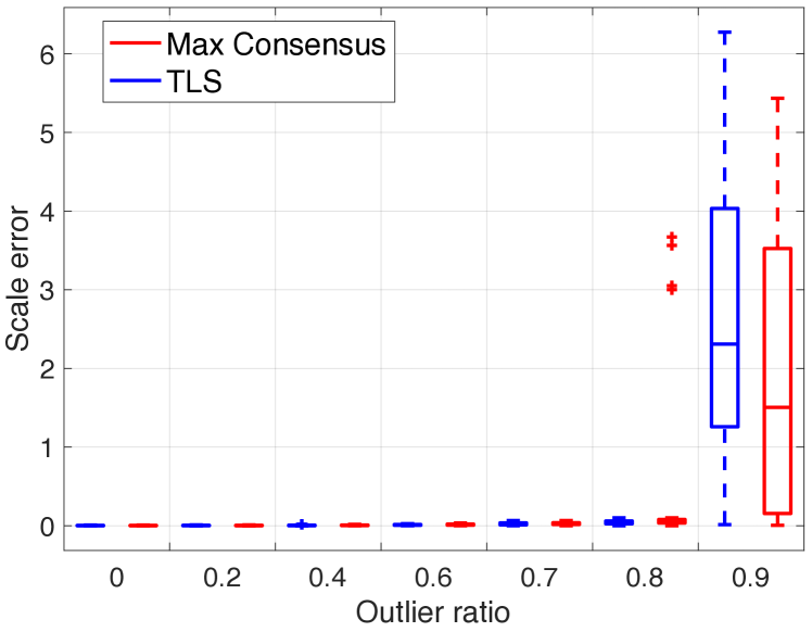
Scale solver. Given two point clouds ${\cal A}$ and ${\cal B}$, we first create $N(N-1)/2$ TIMs corresponding to a complete graph and then use Algorithm 2 to solve for the scale. We compute both maximum consensus [52] and TLS estimates of the scale. Fig. 4(a) shows box plots of the scale error with increasing outlier ratios. The scale error is computed as $|s^{\star}-s_{gt}|$, where $s^{\star}$ is the scale estimate and $s_{gt}$ is the ground-truth . We observe the TLS solver is robust against 80% outliers, while maximum consensus failed three times in that regime.

(a) Scale	(b) Rotation
(c) Translation	(d) MCIS

Figure 4: Results for scale, rotation, translation estimation, and impact of maximal clique pruning for increasing outlier ratios.

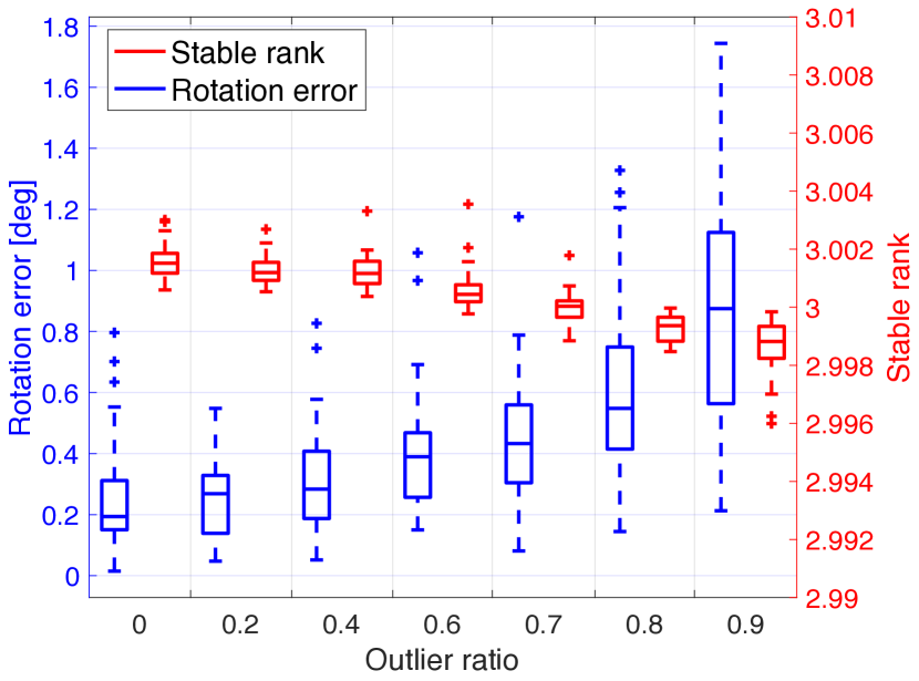
Rotation Solver. We apply a random rotation ${\bm{R}}$ to the Bunny, and fix $s=1$ and ${\bm{t}}={\mathbf{0}}$. Two metrics are boxplotted in Fig. 4(b) to show the performance of the rotation solver: (i) the stable rank of ${\bm{Z}}^{\star}$, the optimal solution of SDP relaxation (20), where the stable rank is defined by the squared ratio between the Frobenius norm and the spectral norm; (ii) the rotation estimation error, defined as $\left|\arccos\left(\left(\mathrm{tr}\left({\bm{R}}_{gt}^{\mathsf{T}}{\bm{R}}^{\star}\right)-1\right)/2\right)\right|$, i.e. the geodesic distance between the rotation estimate ${\bm{R}}^{\star}$ and the ground-truth ${\bm{R}}_{gt}$. We observe the stable rank is numerically close to 3 (Proposition 5) even with 90% of outliers, and the rotation error remains below 2 degrees.

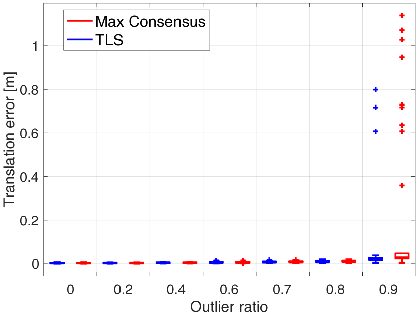
Translation Solver. We apply a random translation ${\bm{t}}$ to the Bunny, and fix $s=1$ and ${\bm{R}}={\mathbf{I}}_{3}$. Fig. 4(c) shows component-wise translation estimation using both maximum consensus and TLS are robust against 80% outliers. The translation error is defined as $\|{\bm{t}}^{\star}-{\bm{t}}_{gt}\|$, the 2-norm of the difference between the estimate ${\bm{t}}^{\star}$ and the ground-truth ${\bm{t}}_{gt}$.

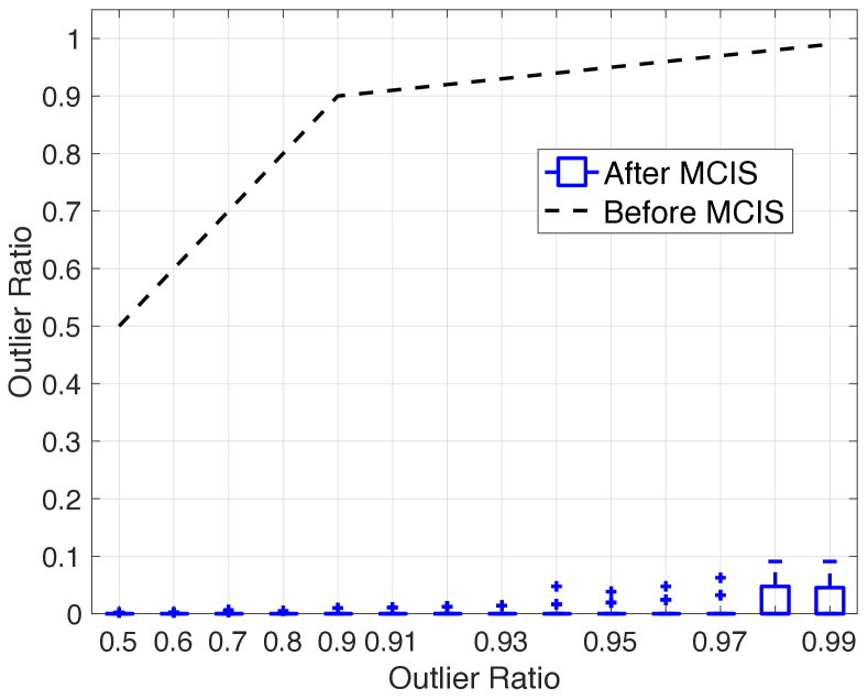
Maximal Clique Inlier Selection. We downsample Bunny to $N=1000$ and fix the scale to $s=1$ when applying the random transformation. We first prune the outlier TIMs/TRIMs (edges) that are not consistent with the scale $s=1$, while keeping all the points (nodes), to obtain the graph ${\cal G}^{\prime}$. Then we compute the maximum clique in ${\cal G}^{\prime}$ using the algorithm in [22], and remove all edges and nodes outside the clique, obtaining a pruned graph ${\cal G}"$. Fig. 4(d) shows the outlier ratio in ${\cal G}^{\prime}$ (label: “Before MCIS”) and ${\cal G}"$ (label: “After MCIS”). The MCIS procedure effectively reduces the amount of outliers to below 10%, facilitating rotation and translation estimation, which, in isolation, can already tolerate more than 90% outliers.

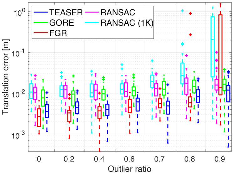(a) Registration with known scale	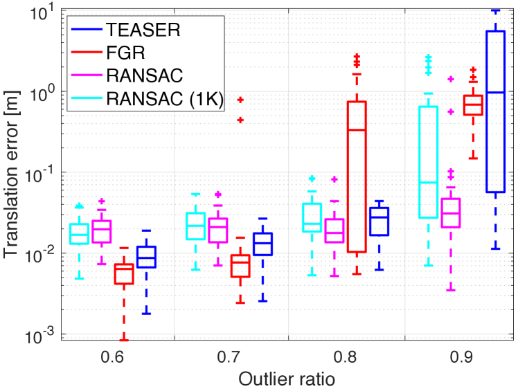(b) Registration with unknown scale	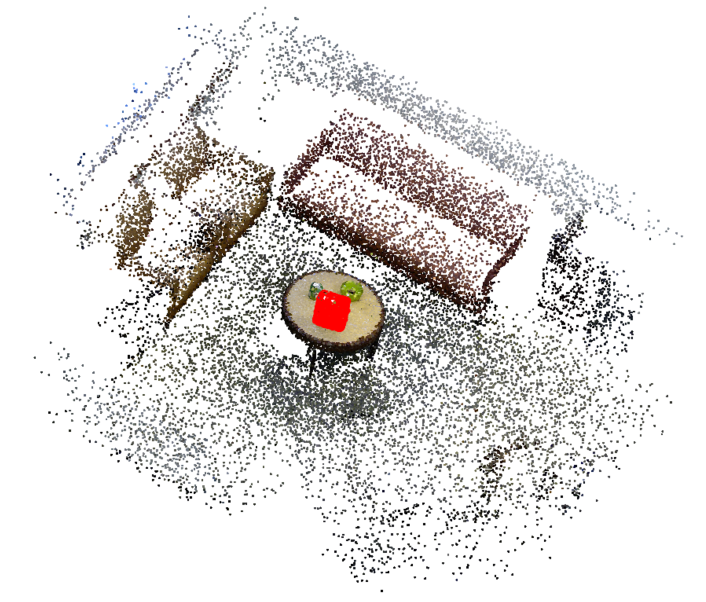(c) Registration on robotics datasets

Figure 5: Benchmark result. (a) Boxplots of rotation and translation errors for the five compared methods on the Bunny dataset with known scale (the top figure shows an example with 50% outliers). (b) Boxplots of scale, rotation and translation errors for four registration methods on the Bunny dataset with unknown scale. (c) Successful object pose estimation by TEASER on a real RGB-D dataset. Blue lines are the original FPFH [50] correspondences with outliers, green lines are the inlier correspondences computed by TEASER, and the final registered object is highlighted in red.

VI-B Benchmarking on Standard Datasets

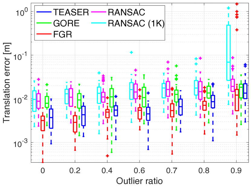
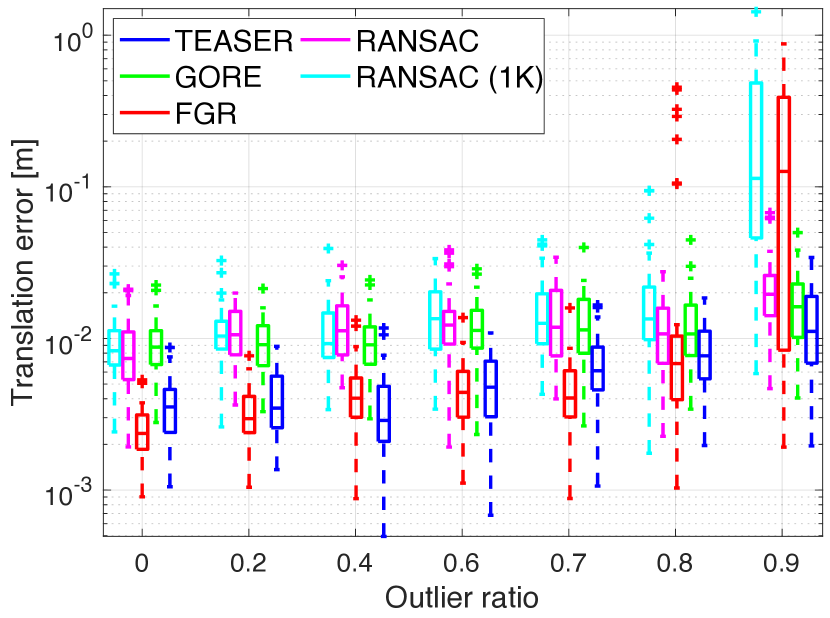
Testing setup. We benchmark TEASER against two state-of-the-art robust registration techniques: Fast Global Registration (FGR) [62] and Guaranteed Outlier REmoval (GORE) [12]. In addition, we test two RANSAC variants: a fast version where we terminate RANSAC after a maximum of 1,000 iterations (RANSAC (1K)) and a slow version where we terminate RANSAC after 60s (RANSAC). Four datasets, Bunny, Armadillo, Dragon and Buddha, from the Stanford 3D Scanning Repository are selected and downsampled to $N=100$ points. The tests below follow the same protocol of Section VI-A. In the Supplementary Material, we provide an example of the performance of TEASER on registration problems with high noise ($\sigma=0.1$).

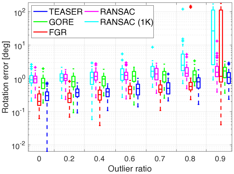
Known Scale. We first evaluate the compared techniques with known scale $s=1$. Fig. 5(a) shows the rotation and translation error at increasing outlier ratios for the Bunny dataset. TEASER, GORE and RANSAC are robust against up to 90% outliers, although TEASER tends to produce more accurate estimates than GORE, and RANSAC typically requires over $10^{5}$ iterations for convergence at 90% outlier rate. FGR can only resist 70% outliers and RANSAC (1K) starts breaking at 60% outlier rate. These conclusions are confirmed by the results on the other three datasets (Armadillo, Dragon, Buddha), which are given in the Supplementary Material due to space constraints.

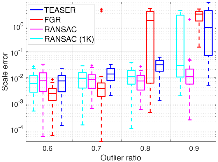
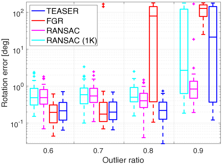
Unknown Scale. GORE is unable to solve for the scale, hence we only benchmark TEASER against FGR (although the original algorithm in [62] did not solve for the scale, we extend it by using Horn’s method to compute the scale at each iteration), RANSAC (1K) and RANSAC. Fig. 5(b) plots the scale, rotation and translation error for increasing outlier ratios on the Bunny dataset. All the compared techniques perform well when the outlier ratio is below 60%. FGR has the lowest breakdown point and fails at 80%. RANSAC (1K) and TEASER only fail at 90% outlier ratio when the scale is unknown. Although RANSAC with 60s timeout outperforms other methods at 90% outlier rate, it typically requires more than $10^{5}$ iterations to converge, which is not practical for real-time applications.

VI-C Testing under Extreme Outlier Rates

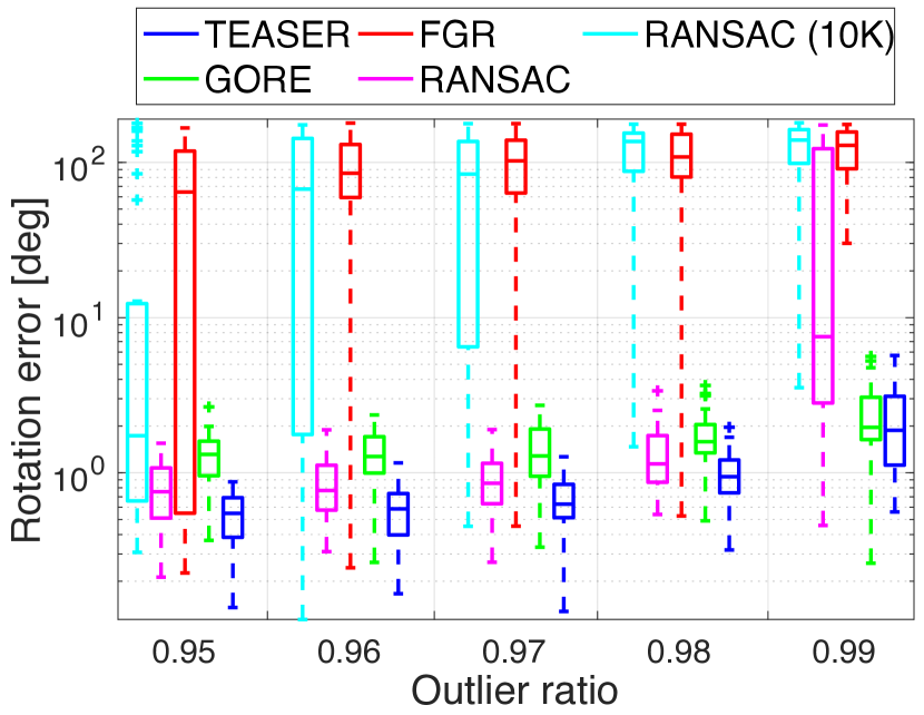
We further benchmark the performance of TEASER under extreme outlier rates from 95% to 99% with known scale and $N=1000$ correspondences on the Bunny. We replace RANSAC (1K) with RANSAC (10K), since RANSAC (1K) already performs poorly at 90% outlier ratio. Fig. 6 shows the boxplots of the rotation and translation errors. Both TEASER and GORE are robust against up to 99% outliers, while RANSAC with 60s timeout can resist 98% outliers with about $10^{6}$ iterations. RANSAC (10K) and FGR perform poorly under extreme outlier ratios. While GORE and TEASER are both robust against 99% outliers, TEASER produces slightly lower estimation errors.

(a) Rotation Error

(b) Translation Error

Figure 6: Estimation errors under extreme outlier rates (known scale).

VI-D Application: Object Pose Estimation and Localization

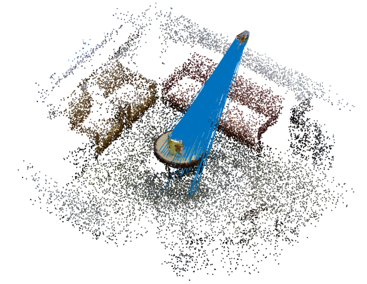
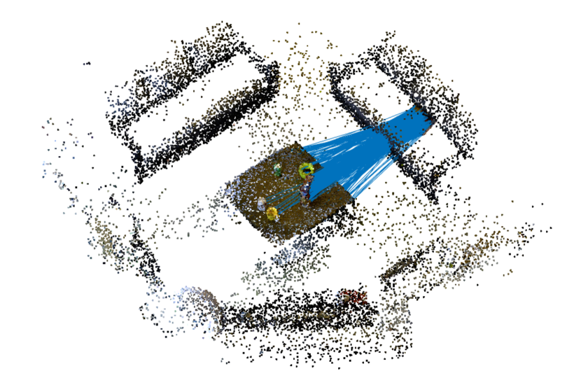
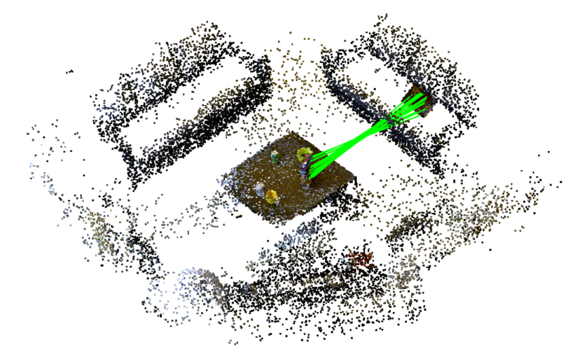
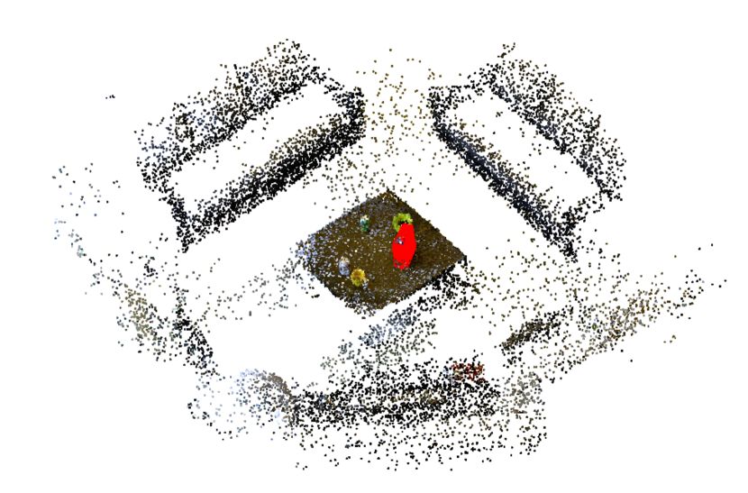
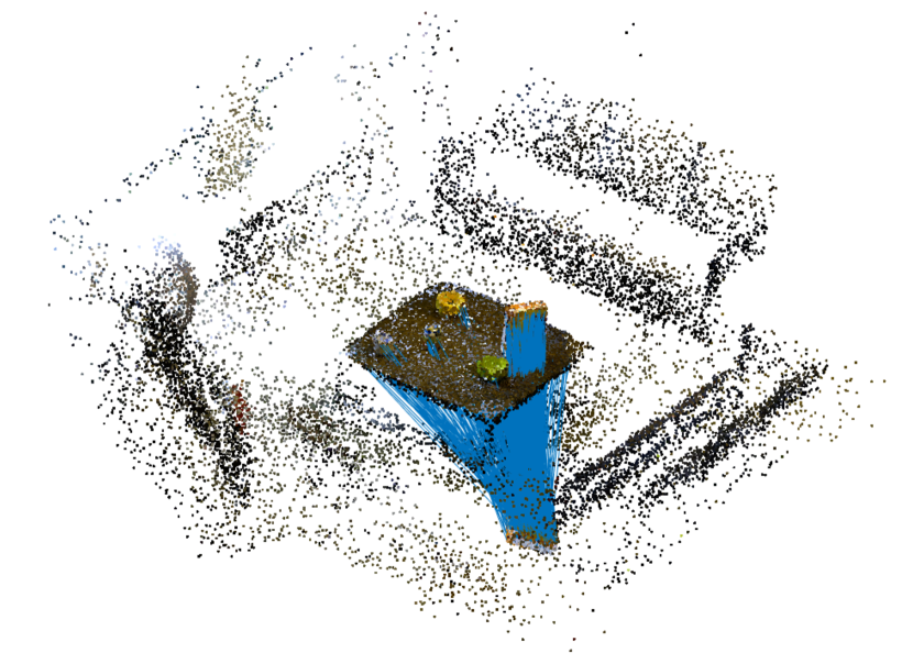
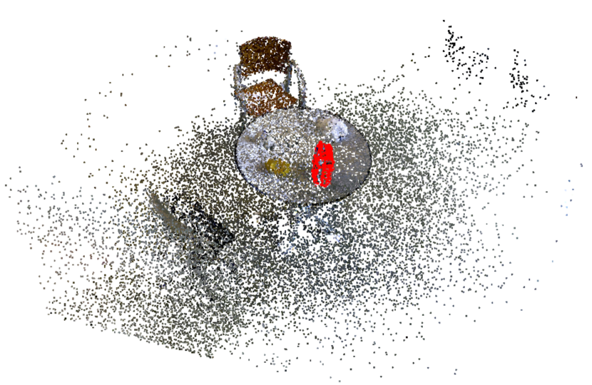
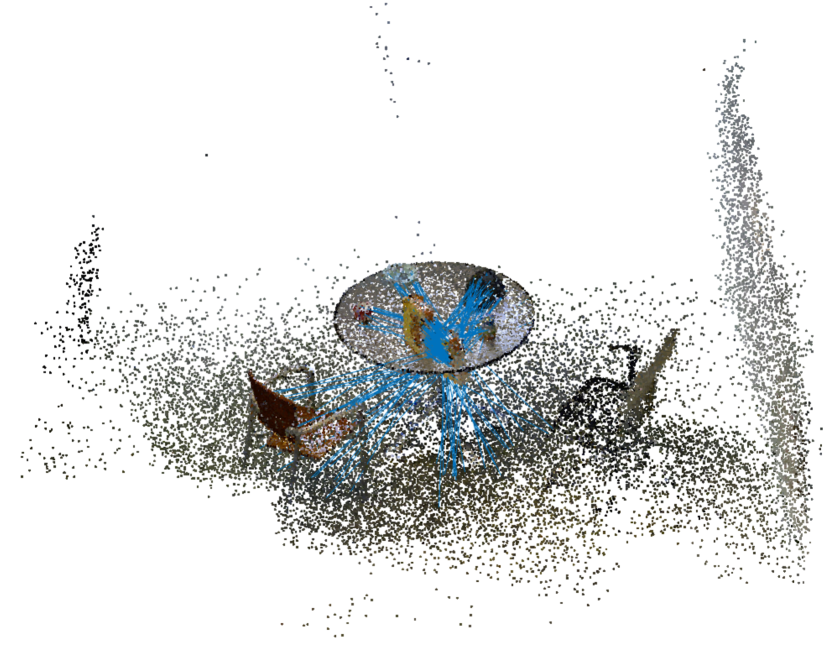
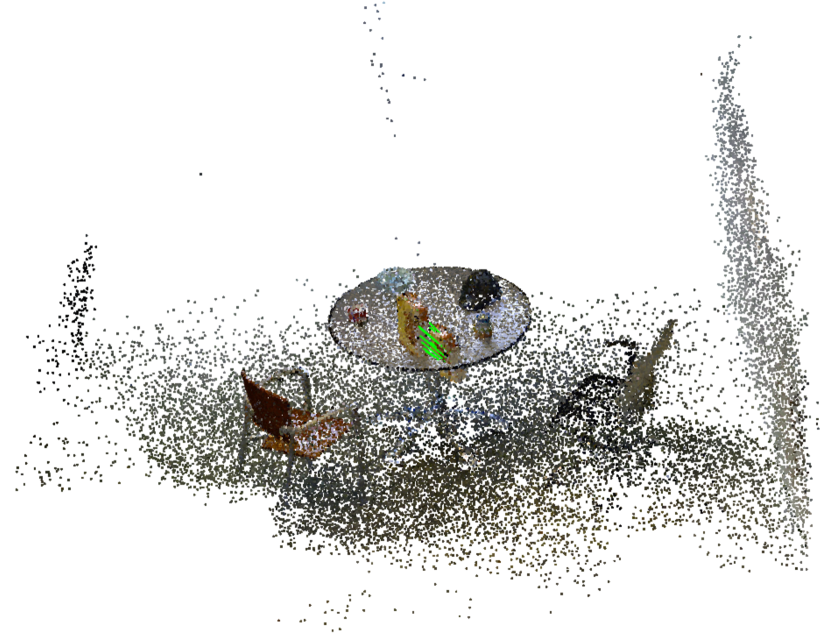
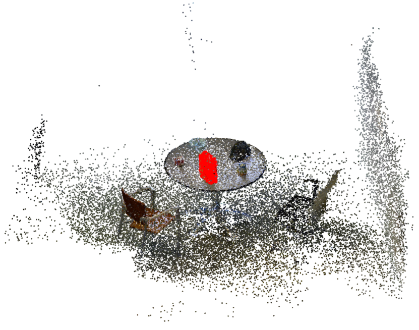
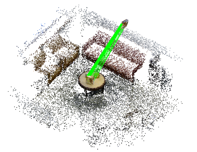
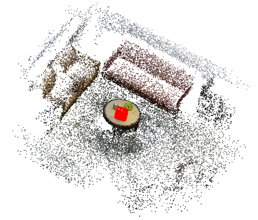
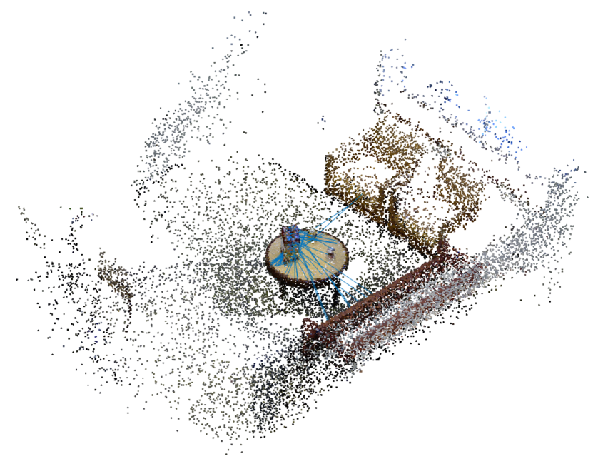
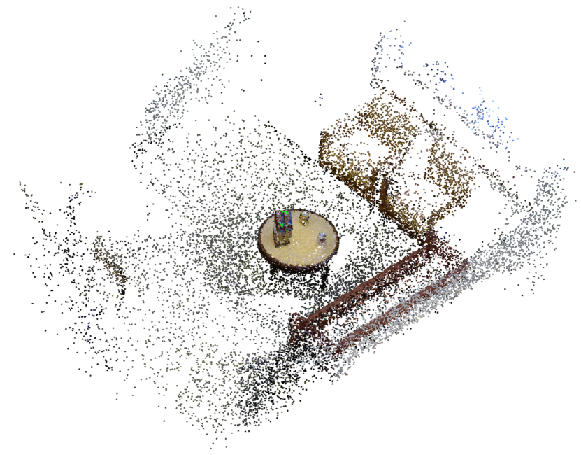
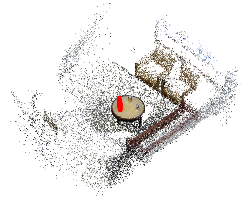
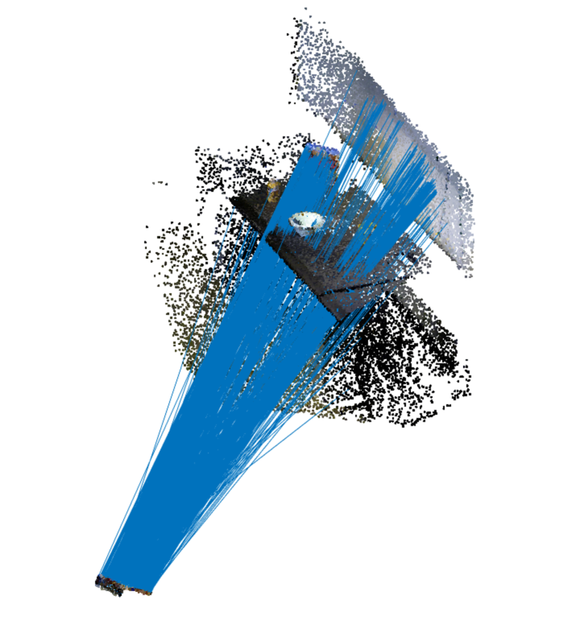
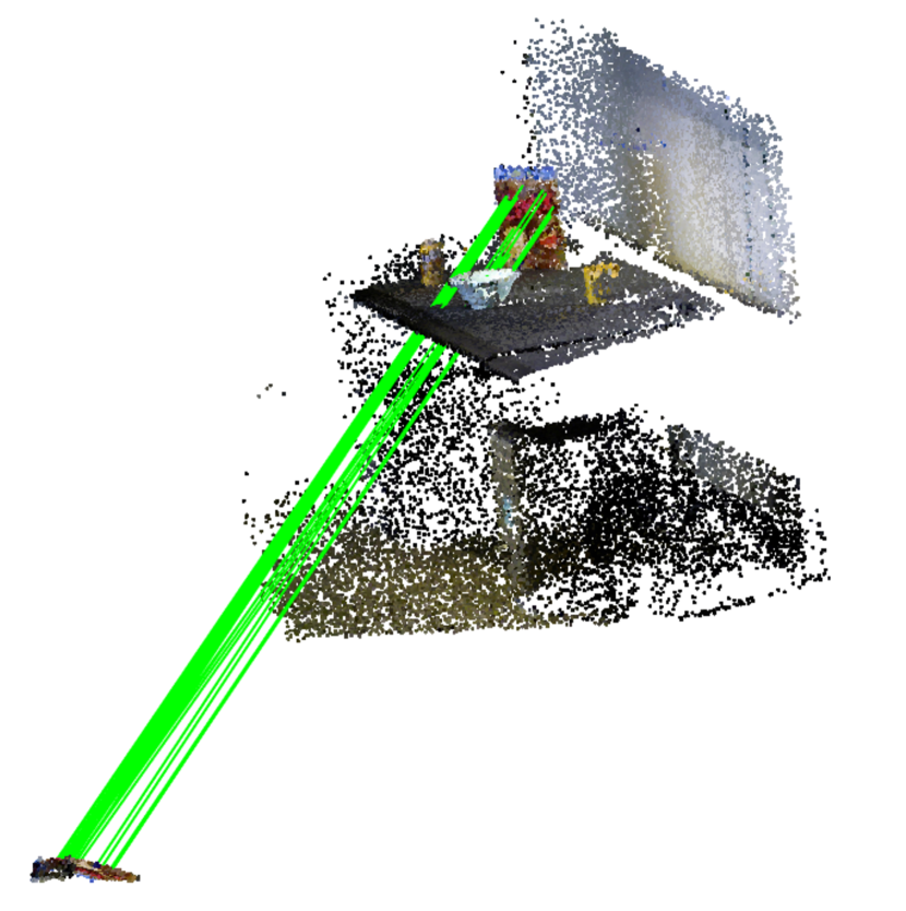
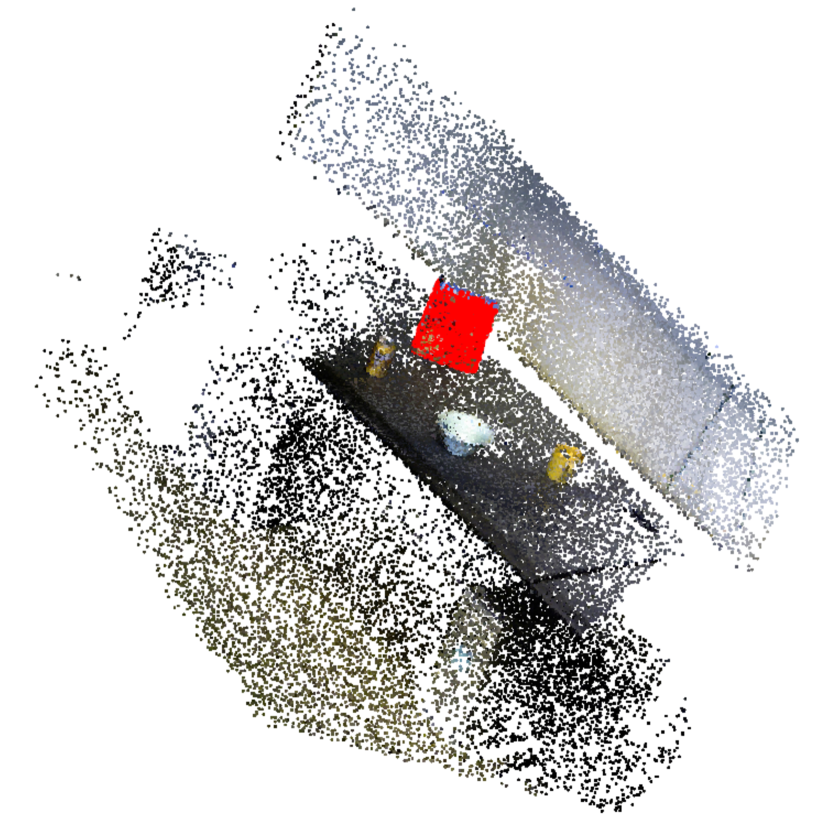
We use the large-scale point cloud datasets from [37] to test TEASER in object pose estimation and localization applications. We first use the ground-truth object labels to extract the cereal box/cap out of the scene and treat it as the object, then apply a random transformation to the scene, to get an object-scene pair. To register the object-scene pair, we first use FPFH feature descriptors [50] to establish putative correspondences. Then, TEASER is used to find the relative pose. Fig. 5(c) shows the noisy FPFH correspondences, the inlier correspondences obtained by TEASER, and successful localization and pose estimation of the cereal box. The Supplementary Material provides results on more object-scene pairs.

VII Conclusion

We propose a Truncated Least Squares approach to compute the relative transformation (scale, rotation, translation) that aligns two point clouds in the presence of extreme outlier rates. We present a general graph-theoretic framework to decouple rotation, translation, and scale estimation. We provide a polynomial-time solution for each subproblem: scale and (component-wise) translation estimation can be solved exactly via an adaptive voting scheme, while rotation estimation can be relaxed to a semidefinite program. The resulting polynomial-time approach , named TEASER (Truncated least squares Estimation And SEmidefinite Relaxation), outperforms RANSAC and robust local optimization techniques, and favorably compares with BnB methods. TEASER can tolerate up to ${99\%}$ outliers and returns highly-accurate solutions.

While running in polynomial time, the general-purpose SDP solver used in our current implementation scales poorly in the problem size. Current research effort is devoted to developing specialized SDP solvers to allow using TEASER to solve large-scale registration problems in real-time.

VIII Proof of Theorem 1

Using the vector notation ${\bm{a}}\in{{\mathbb{R}}^{3N}}$ and ${\bm{b}}\in{{\mathbb{R}}^{3N}}$ already introduced in the statement of the theorem, we can write the generative model (1) compactly as:

$${\bm{b}}=s({\mathbf{I}}_{N}\otimes{\bm{R}}){\bm{a}}+({\mathbf{1}}_{N}\otimes{\bm{t}})+{\bm{o}}+{\bm{\epsilon}}$$ (A22)

where ${\bm{o}}\doteq[{\bm{o}}_{1}^{\mathsf{T}}\;\ldots\;{\bm{o}}_{N}^{\mathsf{T}}]^{\mathsf{T}}$, ${\bm{\epsilon}}\doteq[{\bm{\epsilon}}_{1}^{\mathsf{T}}\;\ldots\;{\bm{\epsilon}}_{N}^{\mathsf{T}}]^{\mathsf{T}}$, and ${\mathbf{1}}_{N}$ is a column vector of ones of size $N$. Denote $K=|{\cal E}|$ as the cadinality of ${\cal E}$, such that ${\bm{A}}\in{{\mathbb{R}}^{K\times N}}$. Let us now multiply both members by $({\bm{A}}\otimes{\mathbf{I}}_{3})$:

$$\bar{{\bm{b}}}=({\bm{A}}\otimes{\mathbf{I}}_{3})[s({\mathbf{I}}_{N}\otimes{\bm{R}}){\bm{a}}+({\mathbf{1}}_{N}\otimes{\bm{t}})+({\bm{o}}+{\bm{\epsilon}})]$$ (A23)

Using the property of the Kronecker product we simplify:

$$\begin{array}[]{ll}(i)&({\bm{A}}\otimes{\mathbf{I}}_{3})({\mathbf{I}}_{N}\otimes{\bm{R}}){\bm{a}}=({\bm{A}}\otimes{\bm{R}}){\bm{a}}\\ &=({\mathbf{I}}_{K}\otimes{\bm{R}})({\bm{A}}\otimes{\mathbf{I}}_{3}){\bm{a}}\\ &=({\mathbf{I}}_{K}\otimes{\bm{R}})\bar{{\bm{a}}}\\ (ii)&({\bm{A}}\otimes{\mathbf{I}}_{3})({\mathbf{1}}_{N}\otimes{\bm{t}})=({\bm{A}}{\mathbf{1}}_{N}\otimes{\bm{t}})={\mathbf{0}}\end{array}$$ (A24)

where we used the fact that ${\mathbf{1}}_{N}$ is in the Null space of the incidence matrix ${\bm{A}}$ [19]. Using (i) and (ii), eq. (A23) becomes:

$$\bar{{\bm{b}}}=s({\mathbf{I}}_{K}\otimes{\bm{R}})\bar{{\bm{a}}}+({\bm{A}}\otimes{\mathbf{I}}_{3})({\bm{o}}+{\bm{\epsilon}})$$ (A25)

which is invariant to the translation ${\bm{t}}$, concluding the proof.

IX Summary of Invariant Measurements

Table A1 below provides a summary of the invariant measurements from the main document.

Measurements	Points	TIMs	TRIMs
Symbol	${\bm{a}}_{i}$, ${\bm{b}}_{i}$	$\bar{{\bm{a}}}_{ij}$, $\bar{{\bm{b}}}_{ij}$	$s_{ij}$
Definition	-	$\begin{cases}\bar{{\bm{a}}}_{ij}=\bar{{\bm{a}}}_{j}-\bar{{\bm{a}}}_{i}\\ \bar{{\bm{b}}}_{ij}=\bar{{\bm{b}}}_{j}-\bar{{\bm{b}}}_{i}\end{cases}$	$s_{ij}=\frac{\|\bar{{\bm{b}}}_{ij}\|}{\|\bar{{\bm{a}}}_{ij}\|}$
Generative model	${\bm{b}}_{i}=s{\bm{R}}{\bm{a}}_{i}+{\bm{t}}+{\bm{o}}_{i}+{\bm{\epsilon}}_{i}$	$\bar{{\bm{b}}}_{ij}=s{\bm{R}}\bar{{\bm{a}}}_{ij}+{\bm{o}}_{ij}+{\bm{\epsilon}}_{ij}$	$s_{ij}=s+o_{ij}^{s}+\epsilon_{ij}^{s}$
Noise bounds	$\|{\bm{\epsilon}}_{i}\|\leq\beta_{i}$	$\|{\bm{\epsilon}}_{ij}\|\leq\beta_{ij}\doteq\beta_{i}+\beta_{j}$	$|\epsilon_{ij}^{s}|\leq\alpha_{ij}\doteq\beta_{ij}/\|\bar{{\bm{a}}}_{ij}\|$
Dependent transformations	$(s,{\bm{R}},{\bm{t}})$	$(s,{\bm{R}})$	s
Number	$N$	$K\leq\frac{N(N-1)}{2}$	$K$

TABLE A1: Summary of invariant measurements.

X Novelty of TIMs and TRIMs

Remark A7 (Novelty).

We remark that the idea of using translation invariant measurements and rotation invariant measurements has been proposed in recent work [39, 12, 40, 1] while (i) the graph theoretic interpretation of Theorem 1 is novel and generalizes previously proposed methods, and (ii) the notion of translation and rotation invariant measurements (TRIMs) is completely new. We also remark that while related work uses invariant measurements to filter-out outliers [12] or to speed up BnB [39, 40], we show that they also allow computing a polynomial-time robust registration solution.

XI Proof of Theorem 2

Let us first prove that there are at most $2K-1$ different non-empty consensus sets. We attach a confidence interval $[s_{k}-\alpha_{k}\bar{c},s_{k}+\alpha_{k}\bar{c}]$ to each measurement $s_{k}$, $\forall k\in\{1,\ldots,K\}$. For a given scalar $s\in{{\mathbb{R}}}$, a measurement $k$ is in the consensus set of $s$ if $s\in[s_{k}-\alpha_{k}\bar{c},s_{k}+\alpha_{k}\bar{c}]$ (satisfies $\frac{\|s-s_{k}\|^{2}}{\alpha_{k}^{2}}\leq\bar{c}^{2}$), see Fig. 3(a). Therefore, the only points on the real line where the consensus set may change are the boundaries (shown in red in Fig. 3(a)) of the intervals $[s_{k}-\alpha_{k}\bar{c},s_{k}+\alpha_{k}\bar{c}]$, $k\in\{1,\ldots,K\}$. Since there are at most $2K-1$ such intervals, there are at most $2K-1$ non-empty consensus sets (Fig. 3(b)), concluding the first part of the proof. The second part follows from the fact that the consensus set of $\hat{s}$ is necessarily one of the $2K-1$ possible consensus sets, and problem (7) simply computes the least squares estimate of the measurements in the consensus set of the solution and choose the estimate that induces the lowest cost as the optimal estimate. Therefore, we can just enumerate every possible consensus set and compute a least squares estimate for each of them, to find the solution that induces the smallest cost.

XII Comments on TLS vs. Consensus Maximization

TLS (and Algorithm 2) are related to consensus maximization, a popular approach for outlier detection in vision [52, 40]. Consensus maximization looks for an estimate that maximizes the number of inliers, i.e. $\max_{s}|{\cal C}(s)|$, where $|\cdot|$ denotes the cardinality of a set. While consensus maximization is intractable in general, by following the same lines of Theorem 2, it is easy to show that consensus maximization can be solved in polynomial time in the scalar case as $\operatorname*{arg\,max}_{i,\ldots,2K-1}|{\cal C}_{i}|$. While we expect the TLS solution to maximize the set of inliers, consensus maximization and TLS will not return the same solution in general, since TLS may prefer to discard measurements that induce a large bias in the estimate, as shown by the simple example below.

Example A8 (TLS vs. Consensus Maximization).

Consider a simple scalar estimation problem, where we are given three measurements $s_{1}\!=\!s_{2}\!=\!0$ and $s_{3}=3$. Assume $\alpha_{k}=2$, $k=1,2,3$ and $\bar{c}=1$. Then, it is possible to see that $s_{m}=1.5$ attains a maximum consensus set including all measurements $\{1,2,3\}$, while the TLS estimate is $\hat{s}=0$ which attains a cost $f_{s}(\hat{s})=1$, and has consensus set ${\cal C}(\hat{s})=\{1,2\}$.

XIII Proof of Theorem 3

Consider a graph ${\cal G}^{\prime}({\cal V},{\cal E}^{\prime})$ whose edges where selected as inliers during scale estimation. An edge $(i,j)$ (and the corresponding TIM) is an inlier if both $i$ and $j$ are correct correspondences (see discussion before Theorem 1). Therefore, ${\cal G}^{\prime}$ contains edges connecting all points for which we have inlier correspondences. Therefore, these points are vertices of a clique in the graph ${\cal G}^{\prime}$ and the edges (or equivalently the TIMs) connecting those points form a clique in ${\cal G}^{\prime}$. We conclude the proof by observing that the clique formed by the inliers has to belong to at least one maximal clique of ${\cal G}^{\prime}$.

XIV Proof of Proposition 4

Here we prove the equivalence between Problem (10) and problem (11). Towards this goal, we show that the latter is simply a reparametrization of the former.

Let us rewrite (10) by making the orthogonality constraint ${\bm{R}}\in\mathrm{O}(3)$ explicit (recall $\mathrm{O}(3)\doteq\{{\bm{R}}\in{{\mathbb{R}}^{3\times 3}}\;{:}\;{\bm{R}}^{\mathsf{T}}{\bm{R}}={\mathbf{I}}_{3}\}$):

$$\min_{\begin{subarray}{c}{\bm{R}},\theta_{k},\forall k\end{subarray}} \sum_{k=1}^{K}\frac{(1+\theta_{k})}{2}\frac{\|\bar{{\bm{b}}}_{k}-{\bm{R}}\bar{{\bm{a}}}_{k}\|^{2}}{\beta^{2}_{k}}+\frac{(1-\theta_{k})}{2}\bar{c}^{2}$$ (A26)

subject to $${\bm{R}}^{\mathsf{T}}{\bm{R}}={\mathbf{I}}_{3},\;\;\theta_{k}\in\{-1,+1\},k=1,\ldots,K$$

Noting that the term $\frac{(1+\theta_{k})}{2}\in\{0,1\}$, we can safely move it inside the squared norm and rewrite eq. (A26) as:

$$\min_{\begin{subarray}{c}{\bm{R}},\theta_{k},\forall k\end{subarray}} \sum_{k=1}^{K}\frac{\|\bar{{\bm{b}}}-{\bm{R}}\bar{{\bm{a}}}+\theta_{k}\bar{{\bm{b}}}-\theta_{k}{\bm{R}}\bar{{\bm{a}}}\|^{2}}{4\beta^{2}_{k}}+\frac{(1-\theta_{k})}{2}\bar{c}^{2}$$ (A27)

subject to $${\bm{R}}^{\mathsf{T}}{\bm{R}}={\mathbf{I}}_{3},\;\;\theta_{k}\in\{-1,+1\},k=1,\ldots,K$$

Now, we reparametrize the problem by introducing matrices ${\bm{R}}_{k}\doteq\theta_{k}{\bm{R}}$. In particular, we note that these matrices satisfy:

• ${\bm{R}}_{k}^{\mathsf{T}}{\bm{R}}_{k}=(\theta_{k}{\bm{R}})^{\mathsf{T}}(\theta_{k}{\bm{R}})=\theta_{k}^{2}{\mathbf{I}}_{3}={\mathbf{I}}_{3}$ (i.e., ${\bm{R}}_{k}\in\mathrm{O}(3)$)

• ${\bm{R}}^{\mathsf{T}}{\bm{R}}_{k}=\theta_{k}\cdot{\mathbf{I}}_{3}\in\{-{\mathbf{I}}_{3},+{\mathbf{I}}_{3}\}$, which also implies

• $\theta_{k}={\bm{e}}_{1}^{\mathsf{T}}{\bm{R}}^{\mathsf{T}}{\bm{R}}_{k}{\bm{e}}_{1}$, where ${\bm{e}}_{1}\doteq[1\;0\;0]^{\mathsf{T}}$.

These three properties allow writing (A27) as:

$$\min_{\begin{subarray}{c}{\bm{R}},{\bm{R}}_{k},\forall k\end{subarray}} \sum_{k=1}^{K}\frac{\|\bar{{\bm{b}}}-{\bm{R}}\bar{{\bm{a}}}+{\bm{R}}^{\mathsf{T}}{\bm{R}}_{k}\bar{{\bm{b}}}-{\bm{R}}_{k}\bar{{\bm{a}}}\|^{2}}{4\beta^{2}_{k}}+\frac{(1-{\bm{e}}_{1}^{\mathsf{T}}{\bm{R}}^{\mathsf{T}}{\bm{R}}_{k}{\bm{e}}_{1})}{2}\bar{c}^{2}$$

subject to $${\bm{R}}^{\mathsf{T}}{\bm{R}}={\mathbf{I}}_{3},\;\;{\bm{R}}_{k}^{\mathsf{T}}{\bm{R}}_{k}={\mathbf{I}}_{3},$$ (A28)

$${\bm{R}}^{\mathsf{T}}{\bm{R}}_{k}\in\{-{\mathbf{I}},+{\mathbf{I}}\},\;k=1,\ldots,K$$

which matches (11), concluding the proof.

XV Proof of Proposition 5

Here we prove that problem (20) is a convex relaxation of (11), in the sense that the two problems have the same objective and the feasible set of (20) contains the feasible set of (11). We start by providing a matrix reparametrization of the problem, given in the following lemma.

Lemma A9 (Matrix ${\bm{X}}$ Formulation).

Problem (11) is equivalent to the following optimization problem:

$$\min_{\begin{subarray}{c}{\bm{X}}\end{subarray}} \mathrm{tr}\left(\bar{{\bm{Q}}}{\bm{X}}^{\mathsf{T}}{\bm{X}}\right)$$ (A29)

subject to $$[{\bm{X}}^{\mathsf{T}}{\bm{X}}]_{RR}={\mathbf{I}}_{3},\;\;\;[{\bm{X}}^{\mathsf{T}}{\bm{X}}]_{R_{k}R_{k}}={\mathbf{I}}_{3},\;\;\;[{\bm{X}}^{\mathsf{T}}{\bm{X}}]_{II}={\mathbf{I}}_{3},$$

$$[{\bm{X}}^{\mathsf{T}}{\bm{X}}]_{RR_{k}}=({\bm{e}}_{1}^{\mathsf{T}}[{\bm{X}}^{\mathsf{T}}{\bm{X}}]_{RR_{k}}{\bm{e}}_{1}){\mathbf{I}}_{3},\;\;\forall k$$

$$\|[{\bm{X}}^{\mathsf{T}}{\bm{X}}]_{IR}\pm[{\bm{X}}^{\mathsf{T}}{\bm{X}}]_{IR_{k}}\|\leq 1\pm({\bm{e}}_{1}^{\mathsf{T}}[{\bm{X}}^{\mathsf{T}}{\bm{X}}]_{RR_{k}}{\bm{e}}_{1}),\;\;\forall k$$

$$\|[{\bm{X}}^{\mathsf{T}}{\bm{X}}]_{IR_{k}}\pm[{\bm{X}}^{\mathsf{T}}{\bm{X}}]_{IR_{k^{\prime}}}\|\leq 1\pm({\bm{e}}_{1}^{\mathsf{T}}[{\bm{X}}^{\mathsf{T}}{\bm{X}}]_{R_{k}R_{k^{\prime}}}{\bm{e}}_{1}),\;\;\forall k,k^{\prime}$$

Proof of Lemma A9. To prove the lemma, we reparametrize problem (11) using the matrix ${\bm{X}}=[{\mathbf{I}}_{3}\;{\bm{R}}\;{\bm{R}}_{1}\;\ldots\;{\bm{R}}_{K}]$.

We first rewrite each summand in the objective of (11) as a quadratic function of ${\bm{X}}$:

$$\begin{array}[]{ll}\frac{\|\bar{{\bm{b}}}_{k}-{\bm{R}}\bar{{\bm{a}}}_{k}+{\bm{R}}^{\mathsf{T}}{\bm{R}}_{k}\bar{{\bm{b}}}_{k}-{\bm{R}}_{k}\bar{{\bm{a}}}_{k}\|^{2}}{4\beta^{2}_{k}}+\frac{(1-{\bm{e}}_{1}^{\mathsf{T}}{\bm{R}}^{\mathsf{T}}{\bm{R}}_{k}{\bm{e}}_{1})}{2}\bar{c}^{2}=\\ \text{\small\color[rgb]{.5,.5,.5}\definecolor[named]{pgfstrokecolor}{rgb}{.5,.5,.5}\pgfsys@color@gray@stroke{.5}\pgfsys@color@gray@fill{.5}(developing the squared norm)}\\ \frac{\|\bar{{\bm{b}}}_{k}-{\bm{R}}\bar{{\bm{a}}}_{k}\|^{2}+\|{\bm{R}}^{\mathsf{T}}{\bm{R}}_{k}\bar{{\bm{b}}}_{k}-{\bm{R}}_{k}\bar{{\bm{a}}}_{k}\|^{2}}{4\beta^{2}_{k}}+\\ \frac{2\mathrm{tr}\left((\bar{{\bm{b}}}_{k}-{\bm{R}}\bar{{\bm{a}}}_{k})^{\mathsf{T}}({\bm{R}}^{\mathsf{T}}{\bm{R}}_{k}\bar{{\bm{b}}}_{k}-{\bm{R}}_{k}\bar{{\bm{a}}}_{k})\right)}{4\beta^{2}_{k}}+\frac{(1-{\bm{e}}_{1}^{\mathsf{T}}{\bm{R}}^{\mathsf{T}}{\bm{R}}_{k}{\bm{e}}_{1})}{2}\bar{c}^{2}=\\ \text{\small\color[rgb]{.5,.5,.5}\definecolor[named]{pgfstrokecolor}{rgb}{.5,.5,.5}\pgfsys@color@gray@stroke{.5}\pgfsys@color@gray@fill{.5}(leveraging that ${\bm{R}}_{k}\in\{-{\bm{R}},+{\bm{R}}\}$ and $\|\pm{\bm{x}}\|=\|{\bm{x}}\|$)}\\ \frac{2\|\bar{{\bm{b}}}_{k}-{\bm{R}}\bar{{\bm{a}}}_{k}\|^{2}}{4\beta^{2}_{k}}+\\ \frac{2\mathrm{tr}\left((\bar{{\bm{b}}}_{k}-{\bm{R}}\bar{{\bm{a}}}_{k})^{\mathsf{T}}({\bm{R}}^{\mathsf{T}}{\bm{R}}_{k}\bar{{\bm{b}}}_{k}-{\bm{R}}_{k}\bar{{\bm{a}}}_{k})\right)}{4\beta^{2}_{k}}+\frac{(1-{\bm{e}}_{1}^{\mathsf{T}}{\bm{R}}^{\mathsf{T}}{\bm{R}}_{k}{\bm{e}}_{1})}{2}\bar{c}^{2}=\\ \text{\small\color[rgb]{.5,.5,.5}\definecolor[named]{pgfstrokecolor}{rgb}{.5,.5,.5}\pgfsys@color@gray@stroke{.5}\pgfsys@color@gray@fill{.5}(developing the first and the second summand)}\\ \frac{\bar{{\bm{b}}}_{k}^{\mathsf{T}}\bar{{\bm{b}}}_{k}+\bar{{\bm{a}}}_{k}^{\mathsf{T}}\bar{{\bm{a}}}_{k}}{2\beta^{2}_{k}}-\frac{2\bar{{\bm{b}}}_{k}^{\mathsf{T}}{\bm{R}}\bar{{\bm{a}}}_{k}}{2\beta^{2}_{k}}+\\ \frac{2\mathrm{tr}\left((\bar{{\bm{b}}}_{k}-{\bm{R}}\bar{{\bm{a}}}_{k})^{\mathsf{T}}({\bm{R}}^{\mathsf{T}}{\bm{R}}_{k}\bar{{\bm{b}}}_{k}-{\bm{R}}_{k}\bar{{\bm{a}}}_{k}\right)}{4\beta^{2}_{k}}+\frac{(1-{\bm{e}}_{1}^{\mathsf{T}}{\bm{R}}^{\mathsf{T}}{\bm{R}}_{k}{\bm{e}}_{1})}{2}\bar{c}^{2}=\\ \text{\small\color[rgb]{.5,.5,.5}\definecolor[named]{pgfstrokecolor}{rgb}{.5,.5,.5}\pgfsys@color@gray@stroke{.5}\pgfsys@color@gray@fill{.5}(developing the product in the trace)}\\ \frac{\bar{{\bm{b}}}_{k}^{\mathsf{T}}\bar{{\bm{b}}}_{k}+\bar{{\bm{a}}}_{k}^{\mathsf{T}}\bar{{\bm{a}}}_{k}}{2\beta^{2}_{k}}-\frac{2\bar{{\bm{b}}}_{k}^{\mathsf{T}}{\bm{R}}\bar{{\bm{a}}}_{k}}{2\beta^{2}_{k}}+\frac{(1-{\bm{e}}_{1}^{\mathsf{T}}{\bm{R}}^{\mathsf{T}}{\bm{R}}_{k}{\bm{e}}_{1})}{2}\bar{c}^{2}+\\ \frac{\mathrm{tr}\left(\bar{{\bm{b}}}_{k}^{\mathsf{T}}{\bm{R}}^{\mathsf{T}}{\bm{R}}_{k}\bar{{\bm{b}}}_{k}-\bar{{\bm{b}}}_{k}^{\mathsf{T}}{\bm{R}}_{k}\bar{{\bm{a}}}_{k}-\bar{{\bm{a}}}_{k}^{\mathsf{T}}{\bm{R}}^{\mathsf{T}}{\bm{R}}^{\mathsf{T}}{\bm{R}}_{k}\bar{{\bm{b}}}_{k}+\bar{{\bm{a}}}_{k}^{\mathsf{T}}{\bm{R}}^{\mathsf{T}}{\bm{R}}_{k}\bar{{\bm{a}}}_{k}\right)}{2\beta^{2}_{k}}=\\ \text{\small\color[rgb]{.5,.5,.5}\definecolor[named]{pgfstrokecolor}{rgb}{.5,.5,.5}\pgfsys@color@gray@stroke{.5}\pgfsys@color@gray@fill{.5}(noting that ${\bm{R}}^{\mathsf{T}}{\bm{R}}^{\mathsf{T}}{\bm{R}}_{k}={\bm{R}}_{k}^{\mathsf{T}}$ and simplifying)}\\ \frac{\bar{{\bm{b}}}_{k}^{\mathsf{T}}\bar{{\bm{b}}}_{k}+\bar{{\bm{a}}}_{k}^{\mathsf{T}}\bar{{\bm{a}}}_{k}}{2\beta^{2}_{k}}-\frac{2\bar{{\bm{b}}}_{k}^{\mathsf{T}}{\bm{R}}\bar{{\bm{a}}}_{k}}{2\beta^{2}_{k}}+\frac{(1-{\bm{e}}_{1}^{\mathsf{T}}{\bm{R}}^{\mathsf{T}}{\bm{R}}_{k}{\bm{e}}_{1})}{2}\bar{c}^{2}+\\ \frac{\mathrm{tr}\left(\bar{{\bm{b}}}_{k}^{\mathsf{T}}{\bm{R}}^{\mathsf{T}}{\bm{R}}_{k}\bar{{\bm{b}}}_{k}-2\bar{{\bm{b}}}_{k}^{\mathsf{T}}{\bm{R}}_{k}\bar{{\bm{a}}}_{k}+\bar{{\bm{a}}}_{k}^{\mathsf{T}}{\bm{R}}^{\mathsf{T}}{\bm{R}}_{k}\bar{{\bm{a}}}_{k}\right)}{2\beta^{2}_{k}}=\\ \end{array}$$

$$\begin{array}[]{ll}\text{\small\color[rgb]{.5,.5,.5}\definecolor[named]{pgfstrokecolor}{rgb}{.5,.5,.5}\pgfsys@color@gray@stroke{.5}\pgfsys@color@gray@fill{.5}(rearranging terms and noting that for $x\in{{\mathbb{R}}},\mathrm{tr}\left(x\right)=x$)}\\ \frac{\bar{{\bm{b}}}_{k}^{\mathsf{T}}\bar{{\bm{b}}}_{k}+\bar{{\bm{a}}}_{k}^{\mathsf{T}}\bar{{\bm{a}}}_{k}+\beta_{k}^{2}\bar{c}^{2}}{2\beta^{2}_{k}}+\frac{(-{\bm{e}}_{1}^{\mathsf{T}}{\bm{R}}^{\mathsf{T}}{\bm{R}}_{k}{\bm{e}}_{1})}{2}\bar{c}^{2}+\\ \frac{\mathrm{tr}\left(\bar{{\bm{b}}}_{k}^{\mathsf{T}}{\bm{R}}^{\mathsf{T}}{\bm{R}}_{k}\bar{{\bm{b}}}_{k}-2\bar{{\bm{b}}}_{k}^{\mathsf{T}}{\bm{R}}_{k}\bar{{\bm{a}}}_{k}-2\bar{{\bm{b}}}_{k}^{\mathsf{T}}{\bm{R}}\bar{{\bm{a}}}_{k}+\bar{{\bm{a}}}_{k}^{\mathsf{T}}{\bm{R}}^{\mathsf{T}}{\bm{R}}_{k}\bar{{\bm{a}}}_{k}\right)}{2\beta^{2}_{k}}=\\ \text{\small\color[rgb]{.5,.5,.5}\definecolor[named]{pgfstrokecolor}{rgb}{.5,.5,.5}\pgfsys@color@gray@stroke{.5}\pgfsys@color@gray@fill{.5}(noting that $x\in{{\mathbb{R}}},\mathrm{tr}\left(x{\mathbf{I}}_{3}\right)=3x$)}\\ \mathrm{tr}\left(\frac{\bar{{\bm{b}}}_{k}^{\mathsf{T}}\bar{{\bm{b}}}_{k}+\bar{{\bm{a}}}_{k}^{\mathsf{T}}\bar{{\bm{a}}}_{k}+\beta_{k}^{2}\bar{c}^{2}}{6\beta^{2}_{k}}{\mathbf{I}}_{3}\right)+\mathrm{tr}\left(-\frac{\bar{c}^{2}}{6}{\bm{R}}^{\mathsf{T}}{\bm{R}}_{k}\right)+\\ \frac{\mathrm{tr}\left(\bar{{\bm{b}}}_{k}^{\mathsf{T}}{\bm{R}}^{\mathsf{T}}{\bm{R}}_{k}\bar{{\bm{b}}}_{k}-2\bar{{\bm{b}}}_{k}^{\mathsf{T}}{\bm{R}}_{k}\bar{{\bm{a}}}_{k}-2\bar{{\bm{b}}}_{k}^{\mathsf{T}}{\bm{R}}\bar{{\bm{a}}}_{k}+\bar{{\bm{a}}}_{k}^{\mathsf{T}}{\bm{R}}^{\mathsf{T}}{\bm{R}}_{k}\bar{{\bm{a}}}_{k}\right)}{2\beta^{2}_{k}}=\\ \text{\small\color[rgb]{.5,.5,.5}\definecolor[named]{pgfstrokecolor}{rgb}{.5,.5,.5}\pgfsys@color@gray@stroke{.5}\pgfsys@color@gray@fill{.5}(using linearity and the cyclic property of the trace)}\\ \mathrm{tr}\left(\frac{\bar{{\bm{b}}}_{k}^{\mathsf{T}}\bar{{\bm{b}}}_{k}+\bar{{\bm{a}}}_{k}^{\mathsf{T}}\bar{{\bm{a}}}_{k}+\beta_{k}^{2}\bar{c}^{2}}{6\beta^{2}_{k}}{\mathbf{I}}_{3}\right)+\mathrm{tr}\left(-\frac{\bar{c}^{2}}{6}{\bm{R}}^{\mathsf{T}}{\bm{R}}_{k}\right)+\\ \mathrm{tr}\left(\frac{1}{2\beta_{k}^{2}}\bar{{\bm{b}}}_{k}\bar{{\bm{b}}}_{k}^{\mathsf{T}}{\bm{R}}^{\mathsf{T}}{\bm{R}}_{k}\right)-\mathrm{tr}\left(\frac{1}{\beta_{k}^{2}}\bar{{\bm{a}}}_{k}\bar{{\bm{b}}}_{k}^{\mathsf{T}}{\bm{R}}_{k}\right)\\ -\mathrm{tr}\left(\frac{1}{\beta_{k}^{2}}\bar{{\bm{a}}}_{k}\bar{{\bm{b}}}_{k}^{\mathsf{T}}{\bm{R}}\right)+\mathrm{tr}\left(\frac{1}{2\beta_{k}^{2}}\bar{{\bm{a}}}_{k}\bar{{\bm{a}}}_{k}^{\mathsf{T}}{\bm{R}}^{\mathsf{T}}{\bm{R}}_{k}\right)\\ \text{\small\color[rgb]{.5,.5,.5}\definecolor[named]{pgfstrokecolor}{rgb}{.5,.5,.5}\pgfsys@color@gray@stroke{.5}\pgfsys@color@gray@fill{.5}(grouping terms including ${\bm{R}}^{\mathsf{T}}{\bm{R}}_{k}$ and using $\mathrm{tr}\left(x{\mathbf{I}}_{3}\right)=3x$)}\\ \mathrm{tr}\left(\frac{\bar{{\bm{b}}}_{k}^{\mathsf{T}}\bar{{\bm{b}}}_{k}+\bar{{\bm{a}}}_{k}^{\mathsf{T}}\bar{{\bm{a}}}_{k}+\beta_{k}^{2}\bar{c}^{2}}{6\beta^{2}_{k}}{\mathbf{I}}_{3}\right)\\ +\mathrm{tr}\left(\frac{\bar{{\bm{b}}}_{k}^{\mathsf{T}}\bar{{\bm{b}}}_{k}+\bar{{\bm{a}}}_{k}^{\mathsf{T}}\bar{{\bm{a}}}_{k}-\beta_{k}^{2}\bar{c}^{2}}{6\beta^{2}_{k}}{\bm{R}}^{\mathsf{T}}{\bm{R}}_{k}\right)\\ -\mathrm{tr}\left(\frac{1}{\beta_{k}^{2}}\bar{{\bm{a}}}_{k}\bar{{\bm{b}}}_{k}^{\mathsf{T}}{\bm{R}}_{k}\right)-\mathrm{tr}\left(\frac{1}{\beta_{k}^{2}}\bar{{\bm{a}}}_{k}\bar{{\bm{b}}}_{k}^{\mathsf{T}}{\bm{R}}\right)\\ \text{\small\color[rgb]{.5,.5,.5}\definecolor[named]{pgfstrokecolor}{rgb}{.5,.5,.5}\pgfsys@color@gray@stroke{.5}\pgfsys@color@gray@fill{.5}(noting that the expression is linear in ${\bm{X}}^{\mathsf{T}}{\bm{X}}$, \emph{cf.} eq.~{}\eqref{eq:Z})}\\ \doteq\bar{{\bm{Q}}}_{k}{\bm{X}}^{\mathsf{T}}{\bm{X}}\end{array}$$

where $\bar{{\bm{Q}}}_{k}$ is a symmetric matrix with $3\times 3$ blocks $[\bar{{\bm{Q}}}_{k}]_{UV}$ (below we use the block indices from eq. (19)) defined as:

$$\;[\bar{{\bm{Q}}}_{k}]_{UV}=\left\{\begin{array}[]{ll}\frac{\bar{{\bm{b}}}_{k}^{\mathsf{T}}\bar{{\bm{b}}}_{k}+\bar{{\bm{a}}}_{k}^{\mathsf{T}}\bar{{\bm{a}}}_{k}+\beta_{k}^{2}\bar{c}^{2}}{6\beta^{2}_{k}}{\mathbf{I}}_{3}&\begin{subarray}{c}\text{if }U=I\text{ and }V=I\end{subarray}\vspace{2mm}\\ \frac{\bar{{\bm{b}}}_{k}^{\mathsf{T}}\bar{{\bm{b}}}_{k}+\bar{{\bm{a}}}_{k}^{\mathsf{T}}\bar{{\bm{a}}}_{k}-\beta_{k}^{2}\bar{c}^{2}}{12\beta^{2}_{k}}{\mathbf{I}}_{3}&\begin{subarray}{c}\text{if }U=R\text{ and }V=R_{k}\\ \text{or }U=R_{k}\text{ and }V=R\end{subarray}\vspace{2mm}\\ -(\frac{1}{2\beta_{k}^{2}}\bar{{\bm{a}}}_{k}\bar{{\bm{b}}}_{k}^{\mathsf{T}})^{\mathsf{T}}&\begin{subarray}{c}\text{if }U=I\text{ and }V=R\\ \text{or }U=I\text{ and }V=R_{k}\end{subarray}\vspace{2mm}\\ -(\frac{1}{2\beta_{k}^{2}}\bar{{\bm{a}}}_{k}\bar{{\bm{b}}}_{k}^{\mathsf{T}})&\begin{subarray}{c}\text{if }U=R\text{ and }V=I\\ \text{or }U=R_{k}\text{ and }V=I\end{subarray}\end{array}\right.$$ (A30)

Since each summand in the objective of (11) can be written as $\bar{{\bm{Q}}}_{k}{\bm{X}}^{\mathsf{T}}{\bm{X}}$, the linearity of the trace allows writing the overall objective as $\bar{{\bm{Q}}}{\bm{X}}^{\mathsf{T}}{\bm{X}}$, where:

$$\bar{{\bm{Q}}}=\sum_{k=1}^{K}\bar{{\bm{Q}}}_{k}$$ (A31)

concluding the first part of the proof.

To finish the proof of the equivalence between (A29) and (11), we show that the constraints in (11) can be written as in (A29), while the latter also includes extra redundant constraints. From the structure of ${\bm{X}}^{\mathsf{T}}{\bm{X}}$ in eq. (19), it is trivial to see that the orthogonality constraints on ${\bm{R}}$ and ${\bm{R}}_{k}$ are equivalent to the first three constraints (first line) in (A29), where we also added a constraint $[{\bm{X}}^{\mathsf{T}}{\bm{X}}]_{II}={\mathbf{I}}_{3}$ on the top-left identity block of ${\bm{X}}^{\mathsf{T}}{\bm{X}}$, cf. eq. (19). Now we note that the constraint ${\bm{R}}^{\mathsf{T}}{\bm{R}}_{k}\in\{-{\mathbf{I}}_{3},+{\mathbf{I}}_{3}\}$ is equivalent to: imposing that (i) ${\bm{R}}^{\mathsf{T}}{\bm{R}}_{k}\in\mathrm{O}(3)$ and (ii) ${\bm{R}}^{\mathsf{T}}{\bm{R}}_{k}=x{\mathbf{I}}_{3}$, for some scalar $x$ (in words, ${\bm{R}}^{\mathsf{T}}{\bm{R}}_{k}$ is a multiple of the identity matrix). This can be easily seen by noting that the two conditions imply:

$$({\bm{R}}^{\mathsf{T}}{\bm{R}}_{k})^{\mathsf{T}}{\bm{R}}^{\mathsf{T}}{\bm{R}}_{k}\overset{(i)}{=}{\mathbf{I}}_{3}\quad\overset{(ii)}{\Rightarrow}\quad x^{2}{\mathbf{I}}_{3}={\mathbf{I}}_{3}$$ (A32)

which is only true for $x\in\{-1,+1\}$. Since we already imposed that ${\bm{R}}$ and ${\bm{R}}_{k}$ are orthogonal, then also ${\bm{R}}^{\mathsf{T}}{\bm{R}}_{k}$ must be orthogonal, and we are only left to add the constraint ${\bm{R}}^{\mathsf{T}}{\bm{R}}_{k}=x{\mathbf{I}}_{3}$. To avoid adding extra variables, we rewrite the constraint ${\bm{R}}^{\mathsf{T}}{\bm{R}}_{k}=x{\mathbf{I}}_{3}$ as:

$$[{\bm{X}}^{\mathsf{T}}{\bm{X}}]_{RR_{k}}=({\bm{e}}_{1}^{\mathsf{T}}[{\bm{X}}^{\mathsf{T}}{\bm{X}}]_{RR_{k}}{\bm{e}}_{1}){\mathbf{I}}_{3}$$ (A33)

where ${\bm{e}}_{1}^{\mathsf{T}}[{\bm{X}}^{\mathsf{T}}{\bm{X}}]_{RR_{k}}{\bm{e}}_{1}$ simply selects the top-left entry of $[{\bm{X}}^{\mathsf{T}}{\bm{X}}]_{RR_{k}}$. Eq. (A33) corresponds to the second line in (A29).

Finally, we note that the last two constraints in (A29) are redundant, i.e., they are trivially satisfied given the other constraints. To prove this fact we observe:

$$\|[{\bm{X}}^{\mathsf{T}}{\bm{X}}]_{IR}\pm[{\bm{X}}^{\mathsf{T}}{\bm{X}}]_{IR_{k}}\|\leq 1\pm({\bm{e}}_{1}^{\mathsf{T}}[{\bm{X}}^{\mathsf{T}}{\bm{X}}]_{RR_{k}}{\bm{e}}_{1}) \iff$$

(using (19))

$$\|{\bm{R}}\pm{\bm{R}}_{k}\|\leq 1\pm({\bm{e}}_{1}^{\mathsf{T}}{\bm{R}}{\bm{R}}_{k}{\bm{e}}_{1}) \iff$$

(recalling $${\bm{R}}_{k}=\theta{\bm{R}} \theta\in\{-1,+1\}$$, for some )

$$\|(1\pm\theta){\bm{R}}\|\leq 1\pm\theta \iff$$

(since $$\|{\bm{R}}\|=1 (1\pm\theta)\geq 0 \theta\in\{-1,+1\}$$ and for )

$$1\pm\theta\leq 1\pm\theta$$ (A34)

which is trivially satisfied (a proof of the redundancy of the last constraint proceeds in a similar manner). $\square$

Remark A10 (Redundant constraints).

The proof of Lemma A9 shows that the last two constraints in (A29) are redundant, i.e., they can be omitted from (A29) without altering the result. While these redundant constraints do not play any role in (A29), empirical evidence shows that they largely improve the quality of our convex relaxation (presented below), and this is the reason why we added them to (A29) in the first place.

We are now ready to prove Proposition 5.

Proof of Proposition 5. Using Lemma A9, it is now trivial to show that (20) is a convex relaxation of (11). Towards this goal, we first observe that from Lemma A9, problem (11) is equivalent to (A29). Second, we observe that (A29) can be rewritten using a matrix ${\bm{Z}}={\bm{X}}^{\mathsf{T}}{\bm{X}}$, which is a positive-semidefinite rank-3 matrix:

$$\min_{\begin{subarray}{c}{\bm{Z}}\end{subarray}} \mathrm{tr}\left(\bar{{\bm{Q}}}{\bm{Z}}\right)$$ (A35)

subject to $$[{\bm{Z}}]_{RR}={\mathbf{I}}_{3},\;\;\;[{\bm{Z}}]_{R_{k}R_{k}}={\mathbf{I}}_{3},\;\;\;[{\bm{Z}}]_{II}={\mathbf{I}}_{3},$$ (A36)

$$[{\bm{Z}}]_{RR_{k}}=({\bm{e}}_{1}^{\mathsf{T}}[{\bm{Z}}]_{RR_{k}}{\bm{e}}_{1}){\mathbf{I}}_{3},\;\;\forall k$$

$$\|[{\bm{Z}}]_{IR}-[{\bm{Z}}]_{IR_{k}}\|\leq 1-({\bm{e}}_{1}^{\mathsf{T}}[{\bm{Z}}]_{RR_{k}}{\bm{e}}_{1}),\;\;\forall k$$

$$\|[{\bm{Z}}]_{IR_{k}}-[{\bm{Z}}]_{IR_{k^{\prime}}}\|\leq 1-({\bm{e}}_{1}^{\mathsf{T}}[{\bm{Z}}]_{R_{k}R_{k^{\prime}}}{\bm{e}}_{1}),\;\;\forall k,k^{\prime}$$

$${\bm{Z}}\succeq 0,\quad\mathrm{rank}\left({\bm{Z}}\right)=3$$

All the constraints in (A35) are convex except the rank constraint. Therefore, we can obtain a convex relaxation by dropping the rank constraint from (A35) and obtain (20). $\square$

XVI Proof of Proposition 6

Here we state and prove an extended version of Proposition 6, which we omitted from the paper for space reasons.

Proposition A11 (Guarantees for TLS Rotation Estimation).

Let ${\bm{Z}}^{\star}$ be the optimal solution of the relaxation (20). The following two facts hold true:

1. If ${\bm{Z}}^{\star}$ has rank 3, then it can be factored as ${\bm{Z}}^{\star}=({\bm{X}}^{\star})^{\mathsf{T}}({\bm{X}}^{\star})$ and the first block row of ${\bm{X}}^{\star}\doteq[{\mathbf{I}}_{3},{{\bm{R}}}^{\star},{{\bm{R}}}^{\star}_{1},\ldots,{{\bm{R}}}^{\star}_{K}]$ is an optimal solution for problem (11).

2. If we call $\hat{{\bm{R}}},\hat{{\bm{R}}}_{1},\ldots,\hat{{\bm{R}}}_{K}$ the rounded estimate, where $\hat{{\bm{R}}}=\text{proj}_{\mathrm{O}(3)}([{\bm{Z}}^{\star}]_{IR})$ ($\text{proj}_{S}$ is the projection onto a set $S$), and $\hat{{\bm{R}}}_{k}=\text{proj}_{\{-\hat{{\bm{R}}},+\hat{{\bm{R}}}\}}([{\bm{Z}}^{\star}]_{IR_{k}})$, then the rounded estimate is feasible for the original problem (11), and the suboptimality of the rounded estimate is bounded by:

   $$\hat{f}_{R}-f_{R}^{\star}\leq\hat{f}_{R}-f_{R}^{\circ}$$ (A37)

   where $f_{R}^{\star}$ is the optimal objective of (11), $\hat{f}_{R}$ is the objective attained in (11) by the rounded estimate, and $f_{R}^{\circ}$ is the optimal objective of the convex relaxation (20).

Proof. We first observe that $f_{R}^{\circ}\leq f_{R}^{\star}$: by definition, a relaxation can only attain a better objective with respect to the original problem, since it operates on a larger feasible set.

Now we prove the first claim in Proposition A11. The proof easily follows from Lemma A9 and the proof of Proposition 5. In particular, in the proof of Proposition 5, we showed that (i) problem (11) is equivalent to problem (A35), and (ii) (A35) is the same as the convex relaxation (20), except from the fact that in the relaxation we dropped the rank constraint. Therefore, if the relaxation (20) produces a rank-3 solution, such solution is also optimal for (A35) (such solution attains a cost $f_{R}^{\circ}\leq f_{R}^{\star}$, hence when it is feasible, it must be optimal). Moreover, since such solution is rank 3, it can be factored as ${\bm{Z}}^{\star}=({\bm{X}}^{\star})^{\mathsf{T}}({\bm{X}}^{\star})$ and ${\bm{X}}^{\star}$ solves (A29). Since (A29) is a reparametrization of the original problem (11), we can always build an optimal solution to (11) using the blocks of ${\bm{X}}^{\star}$, concluding the proof of the first claim.

The second claim follows from the fact that (i) the rounded estimate satisfies the constraints in (11), hence must be feasible, and (ii) $f_{R}^{\circ}\leq f_{R}^{\star}$ (already observed earlier in the proof). Using (ii) we obtain:

$$f_{R}^{\circ}\leq f_{R}^{\star}\Rightarrow-f_{R}^{\star}\leq-f_{R}^{\circ}$$

(adding $$\hat{f}_{R}$$ to both members)

$$\Rightarrow\hat{f}_{R}-f_{R}^{\star}\leq\hat{f}_{R}-f_{R}^{\circ}$$ (A38)

which concludes the proof.

Remark A12 (Rounding).

The projections required to compute the rounded solution can be computed efficiently. In particular, for any matrix ${\bm{M}}\in{{\mathbb{R}}^{3\times 3}}$, $\text{proj}_{\mathrm{O}(3)}({\bm{M}})$ can be computed via SVD [28], while $\text{proj}_{\{-\hat{{\bm{R}}},+\hat{{\bm{R}}}\}}({\bm{M}})$ can be computed by inspection since the set $\{-\hat{{\bm{R}}},+\hat{{\bm{R}}}\}$ only contains two elements.

XVII Robust Translation Estimation

After obtaining an estimate of the scale $\hat{s}$ and the rotation $\hat{{\bm{R}}}$, we can substitute them into the original formulation (2) and solve the resulting optimization problem to compute an estimate of the translation ${\bm{t}}$. Since we already presented a poly-time solution for scalar TLS in Section V-A, we propose to solve for the translation component-wise, i.e., we compute the entries $t_{1},t_{2},t_{3}$ of ${\bm{t}}$ independently as the minimizers of:

$$\min_{\begin{subarray}{c}t_{j}\end{subarray}}\sum_{i=1}^{N}\min\left(\frac{1}{\beta_{i}^{2}}\left|[{\bm{b}}_{i}-\hat{s}\hat{{\bm{R}}}{\bm{a}}_{i}]_{j}-t_{j}\right|^{2}\!\!,\bar{c}^{2}\right)$$ (A39)

where $[\cdot]_{j}$, $j=1,2,3$, denotes the $j$-th entry of a vector. While the solution to (A39) will not match in general the solution to (2), problem (A39) also has the effect to bound the maximum admissible error for each inlier measurement to $\beta_{i}$, but while (2) operates on the $\ell_{2}$ norm of the vector, operates component-wise (A39) (in other words, while the error in our original noise model was confined within the $\ell_{2}$-norm ball, it has been now relaxed to the $\ell_{\infty}$-norm ball).

(a) Armadillo	(b) Dragon	(c) Buddha

Figure A7: Results for the Armadillo, Dragon and Buddha datasets at increasing levels of outliers. First row: example of putative correspondences with 50% outliers. Blue points are the model point cloud, red points are the transformed scene model. Second row: rotation error produced by five methods including TEASER. Third row: translation error produced by the five methods.

XVIII Experiments and Applications

In all the following experiments, $\bar{c}^{2}=1$ for scale, rotation and translation estimation.

XVIII-A Benchmark on Synthetic Datasets

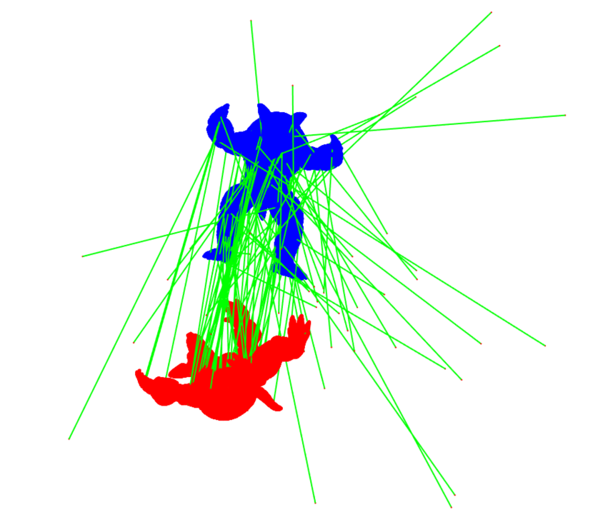
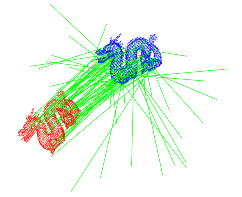
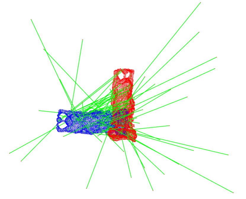
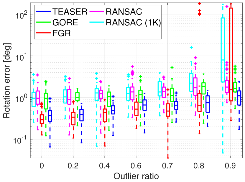
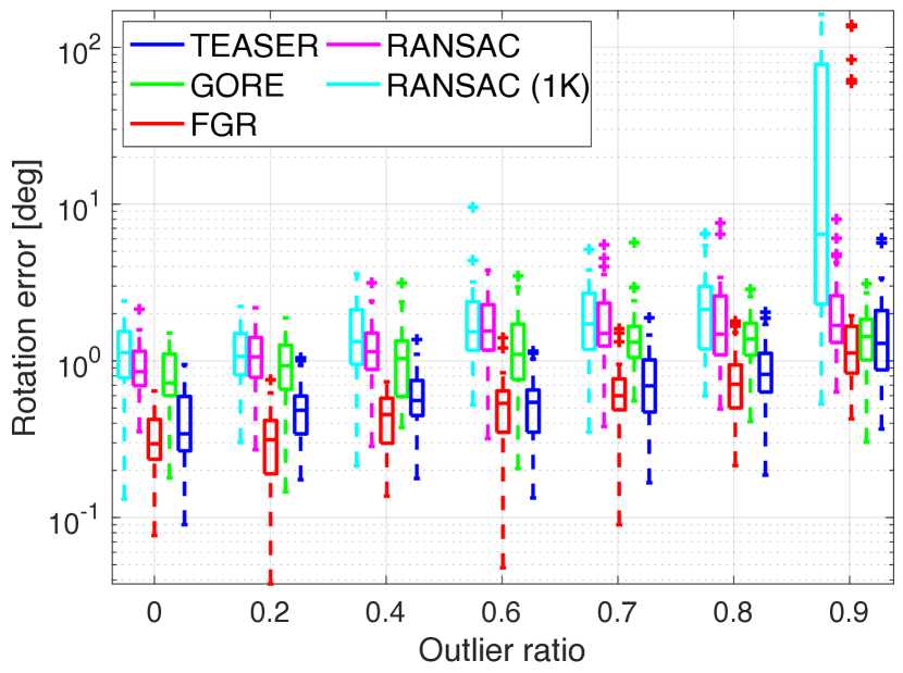
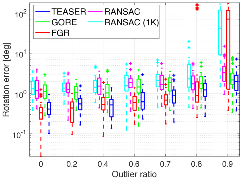
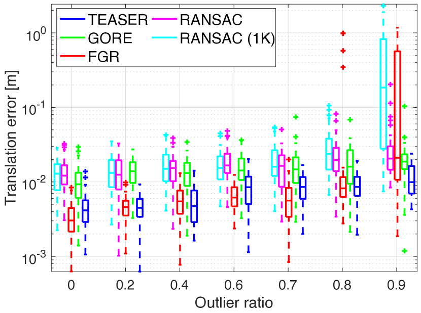
As stated in Section VI-B in the main document, we have benchmarked TEASER against four state-of-the-art methods in point cloud registration (FGR [62], GORE [12], RANSAC (1K), RANSAC) at increasing level of outliers, using four datasets from the Stanford 3D Scanning Repository [20]: Bunny, Armadillo, Dragon and Buddha. Results for the Bunny are showed in the main document and here we show the results for the other three datasets in Fig. A7.

XVIII-B TEASER on High Noise

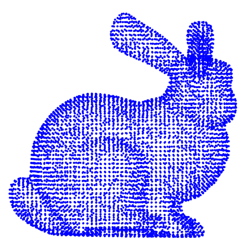
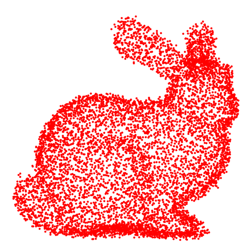
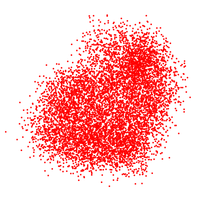
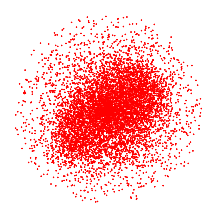
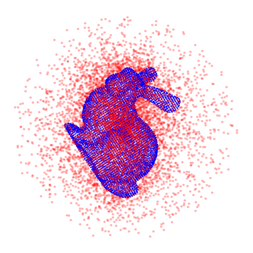
In the main document, the standard deviation $\sigma$ of the isotropic Gaussian noise is set to be $0.01$, with the point cloud scaled inside a unit cube $[0,1]^{3}$. In this section, we give a visual illustration of how corrupted the point cloud is after adding noise of such magnitude. In addition, we increase the noise standard deviation $\sigma$ to be $0.1$, visualize the corresponding corrupted point cloud and show that TEASER can still recover the ground-truth transformation with reasonable accuracy. Fig. A8 illustrates a clean (noise-free) Bunny model scaled inside the unit cube and its variants by adding different levels of isotropic Gaussian noise and outliers. From Fig. A8(b)(c), we can see $\sigma=0.01$ (noise used in the main document) is a reasonable noise standard deviation for real-world applications, while $\sigma=0.1$ destroys the geometric structure of the Bunny and it is beyond the noise typically encountered in robotics and computer vision applications.

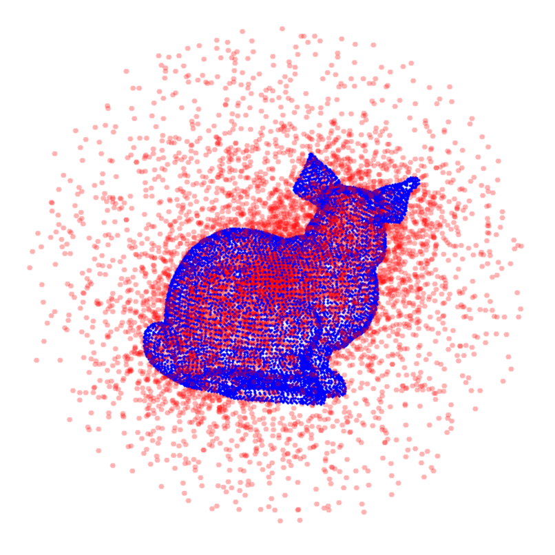
Fig. A8(d) shows the Bunny with high noise ($\sigma=0.1$) and 50% outliers. Under this setup, we run TEASER to register the two point clouds and recover the relative transformation. TEASER can still return rotation and translation estimates that are close to the ground-truth transformation. However, due to the severe noise corruption, even a successful registration fails to yield a visually convincing registration result to human perception. For example, Fig. A9 shows a representative TEASER registration result with $\sigma=0.1$ noise corruption and $50\%$ outlier rate, where accurate transformation estimates are obtained (rotation error is $3.42^{\circ}$ and translation error is $0.098$m), but the Bunny in the cluttered scene is hardly visible, even when super-imposed to the clean model.

(a) Bunny model	(b) Bunny scene, $\sigma=0.01$
(c) Bunny scene, $\sigma=0.1$	(d) Bunny scene, $\sigma=0.1$, 50% outliers

Figure A8: Bunny point cloud scaled inside unit cube $[0,1]^{3}$ and corrupted by different levels of noise and outliers, all viewed from the same perspective angle. (a) Clean Bunny model point cloud, scaled inside unit cube $[0,1]^{3}$. (b) Bunny scene, generated from (a) by adding isotropic Gaussian noise with standard deviation $\sigma=0.01$. (c) Bunny scene, generated from (a) by adding isotropic Gaussian noise with $\sigma=0.1$. (d) Bunny scene, generated from (a) by adding isotropic Gaussian noise with $\sigma=0.1$ and $50\%$ random outliers.

Figure A9: A single representative TEASER registration result with $\sigma=0.1$ noise corruption and $50\%$ outliers, viewed from two distinctive perspectives. Clean Bunny model showed in blue and cluttered scene showed in red. Although the rotation error compared to ground-truth is $3.42^{\circ}$ and the translation error compared to ground-truth is $0.098$m, it is challenging for a human to confirm the correctness of the registration result.

XVIII-C Object Localization and Pose Estimation

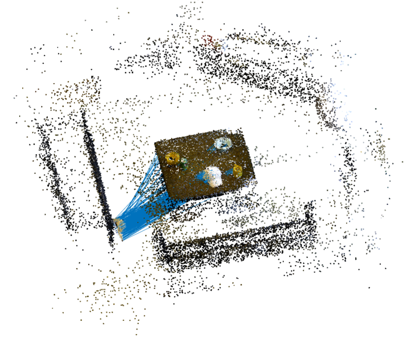
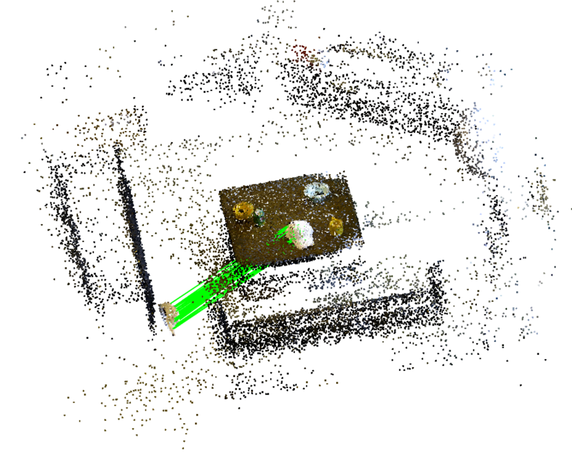
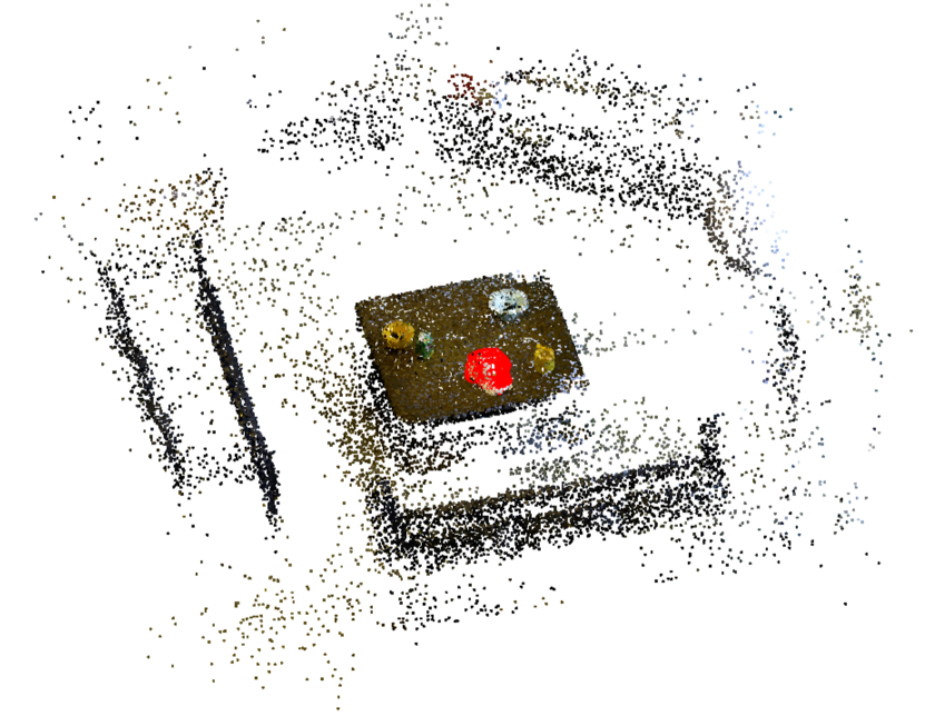
We use the large-scale point cloud datasets from the University of Washington [37] to test TEASER in object pose estimation applications. Seven scenes containing a cereal box and one scene containing a cap are selected from the dataset. We first use the ground-truth object labels to extract the cereal box/cap out of the scene and treat it as the object, then apply a random rotation and translation to the scene, to get an object-scene pair. To register the object-scene pair of point clouds, we first use FPFH feature descriptors [50] as implemented in the Point Cloud Library (PCL) to establish putative feature correspondences. Given correspondences from FPFH, TEASER is used to find the relative pose between the object and scene. We downsample the object and scene using the same ratio (about 0.1) to make the object have 2,000 points, so that FPFH and TEASER can run in reasonable time. Fig. A10 shows the registration results for all 8 selected scenes. The inlier correspondence ratios for cereal box are all below 10% and typically below 5%. TEASER is able to compute a highly-accurate estimate of the relative pose using a handful of inliers. Due to the distinctive shape of cap, FPFH produces a higher number of inliers and TEASER is able to register the object-scene pair without problems. Table A2 shows the mean and standard deviation (STD) of the rotation and translation errors, the number of FPFH correspondences, and the FPFH inlier ratio estimated by TEASER on the eight scenes.

	Rotation error [rad]	Translation error [m]	# of FPFH correspondences	FPFH inlier ratio [%]
Mean	0.0665	0.0695	525	6.53
STD	0.0435	0.0526	161	4.59

TABLE A2: Registration results on eight scenes of the RGB-D dataset [37].

scene-2, # of FPFH correspondences: 550, Inlier ratio: 4.55%, Rotation error: 0.120, Translation error: 0.052.
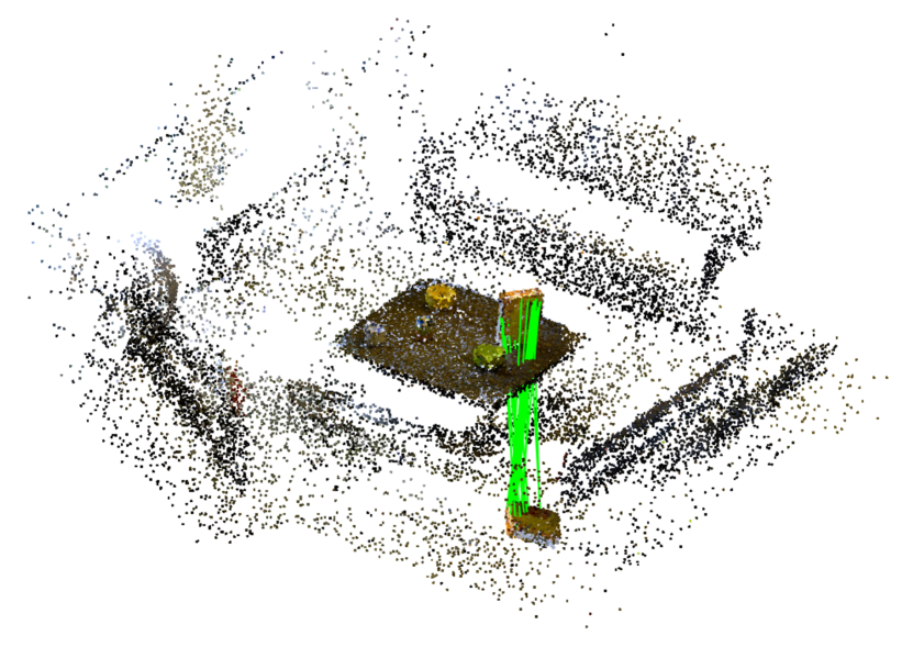
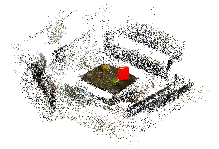
scene-4, # of FPFH correspondences: 636, Inlier ratio: 4.56%, Rotation error: 0.042, Translation error: 0.051.
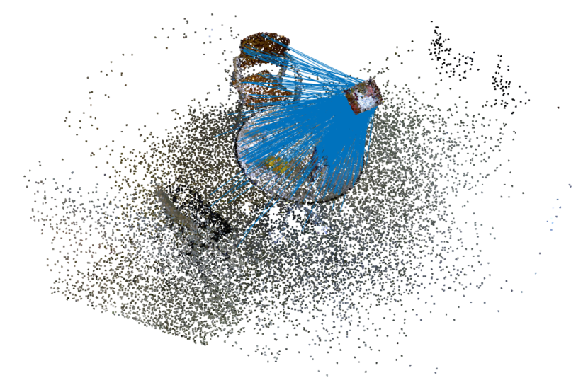
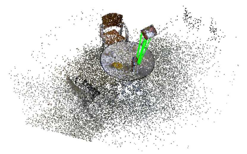
scene-5, # of FPFH correspondences: 685, Inlier ratio: 2.63%, Rotation error: 0.146, Translation error: 0.176.
scene-7, # of FPFH correspondences: 416, Inlier ratio: 3.13%, Rotation error: 0.058, Translation error: 0.097.

Figure A10: Object pose estimation on the large-scale RGB-D dataset [37]. First column: FPFH correspondences, second column: inlier correspondences after TEASER, third column: registration result with the registered object highlighted in red. Scene number and related registration information are listed below each scene.

scene-9, # of FPFH correspondences: 651, Inlier ratio: 8.29%, Rotation error: 0.036, Translation error: 0.011.
scene-11, # of FPFH correspondences: 445, Inlier ratio: 6.97%, Rotation error: 0.028, Translation error: 0.016.
scene-13, # of FPFH correspondences: 612, Inlier ratio: 5.23%, Rotation error: 0.036, Translation error: 0.064.
scene-1, # of FPFH correspondences: 207, Inlier ratio: 16.91%, Rotation error: 0.066, Translation error: 0.090.

Figure A10: Object pose estimation on the large-scale RGB-D dataset [37] (cont.).

References

- Agarwal et al. [2017] S. Agarwal, V. Shree, and S. Chakravorty. RFM-SLAM: Exploiting relative feature measurements to separate orientation and position estimation in slam. In IEEE Intl. Conf. on Robotics and Automation (ICRA), pages 6307–6314. IEEE, 2017.
- Arun et al. [1987] K. S. Arun, T. S. Huang, and S. D. Blostein. Least-squares fitting of two 3-D point sets. IEEE Trans. Pattern Anal. Machine Intell., 9(5):698 –700, sept. 1987.
- Audette et al. [2000] M. A. Audette, F. P. Ferrie, and T. M. Peters. An algorithmic overview of surface registration techniques for medical imaging. Med. Image Anal., 4(3):201–217, 2000.
- Bazin et al. [2014] J. C. Bazin, Y. Seo, R. I. Hartley, and M. Pollefeys. Globally optimal inlier set maximization with unknown rotation and focal length. In European Conf. on Computer Vision (ECCV), pages 803–817, 2014.
- Besl and McKay [1992] P. J. Besl and N. D. McKay. A method for registration of 3-D shapes. IEEE Trans. Pattern Anal. Machine Intell., 14(2), 1992.
- Black and Rangarajan [1996] M. J. Black and A. Rangarajan. On the unification of line processes, outlier rejection, and robust statistics with applications in early vision. Intl. J. of Computer Vision, 19(1):57–91, 1996.
- Blais and Levine [1995] G. Blais and M. D. Levine. Registering multiview range data to create 3d computer objects. IEEE Trans. Pattern Anal. Machine Intell., 17(8):820–824, 1995.
- Bouaziz et al. [2013] S. Bouaziz, A. Tagliasacchi, and M. Pauly. Sparse iterative closest point. In ACM Symp. Geom. Process., pages 113–123. Eurographics Association, 2013.
- Breuel [2003] T. M. Breuel. Implementation techniques for geometric branch-and-bound matching methods. Comput. Vis. Image Underst., 90(3):258–294, 2003.
- Briales and Gonzalez-Jimenez [2017] J. Briales and J. Gonzalez-Jimenez. Convex Global 3D Registration with Lagrangian Duality. In IEEE Conf. on Computer Vision and Pattern Recognition (CVPR), 2017.
- Bron and Kerbosch [1973] C. Bron and J. Kerbosch. Algorithm 457: finding all cliques of an undirected graph. Communications of the ACM, 16(9):575–577, 1973.
- Bustos and Chin [2018] Á. P. Bustos and T. J. Chin. Guaranteed outlier removal for point cloud registration with correspondences. IEEE Trans. Pattern Anal. Machine Intell., 40(12):2868–2882, 2018.
- Bustos et al. [2014] A. Parra Bustos, T. J. Chin, and D. Suter. Fast rotation search with stereographic projections for 3d registration. In IEEE Conf. on Computer Vision and Pattern Recognition (CVPR), pages 3930–3937, 2014.
- Campbell and Petersson [2015] D. Campbell and L. Petersson. An adaptive data representation for robust point-set registration and merging. In Intl. Conf. on Computer Vision (ICCV), pages 4292–4300, 2015.
- Campbell and Petersson [2016] D. Campbell and L. Petersson. Gogma: Globally-optimal gaussian mixture alignment. In IEEE Conf. on Computer Vision and Pattern Recognition (CVPR), pages 5685–5694, 2016.
- Chen et al. [1999] C. S. Chen, Y. P. Hung, and J. B. Cheng. RANSAC-based DARCES: A new approach to fast automatic registration of partially overlapping range images. IEEE Trans. Pattern Anal. Machine Intell., 21(11):1229–1234, 1999.
- Chetverikov et al. [2005] D. Chetverikov, D. Stepanov, and P. Krsek. Robust euclidean alignment of 3d point sets: the trimmed iterative closest point algorithm. Image and Vision Computing, 23(3):299–309, 2005.
- Choi et al. [2015] S. Choi, Q. Y. Zhou, and V. Koltun. Robust reconstruction of indoor scenes. In IEEE Conf. on Computer Vision and Pattern Recognition (CVPR), pages 5556–5565, 2015.
- Chung [1996] F.R.K. Chung. Spectral Graph Theory. American Mathematical Soc., CBMS Regional Conference Series in Mathematics, No. 92, 1996.
- Curless and Levoy [1996] B. Curless and M. Levoy. A volumetric method for building complex models from range images. In SIGGRAPH, pages 303–312, 1996.
- Drost et al. [2010] B. Drost, M. Ulrich, N. Navab, and S. Ilic. Model globally, match locally: Efficient and robust 3D object recognition. In IEEE Conf. on Computer Vision and Pattern Recognition (CVPR), pages 998–1005, 2010.
- Eppstein et al. [2010] D. Eppstein, M. Löffler, and D. Strash. Listing all maximal cliques in sparse graphs in near-optimal time. In International Symposium on Algorithms and Computation, pages 403–414. Springer, 2010.
- Fischler and Bolles [1981] M. Fischler and R. Bolles. Random sample consensus: a paradigm for model fitting with application to image analysis and automated cartography. Commun. ACM, 24:381–395, 1981.
- Granger and Pennec [2002] S. Granger and X. Pennec. Multi-scale EM-ICP: A fast and robust approach for surface registration. In European Conf. on Computer Vision (ECCV), 2002.
- [25] M. Grant and S. Boyd. CVX: Matlab software for disciplined convex programming. URL http://cvxr.com/cvx.
- Guo et al. [2014] Y. Guo, M. Bennamoun, F. Sohel, M. Lu, and J. Wan. 3D object recognition in cluttered scenes with local surface features: a survey. IEEE Trans. Pattern Anal. Machine Intell., 36(11):2270–2287, 2014.
- Hartley and Zisserman [2000] R. Hartley and A. Zisserman. Multiple View Geometry in Computer Vision. Cambridge University Press, 2000.
- Hartley et al. [2013] R. Hartley, J. Trumpf, Y. Dai, and H. Li. Rotation averaging. IJCV, 103(3):267–305, 2013.
- Hartley and Kahl [2009] R. I. Hartley and F. Kahl. Global optimization through rotation space search. Intl. J. of Computer Vision, 82(1):64–79, 2009.
- Henry et al. [2012] P. Henry, M. Krainin, E. Herbst, X. Ren, and D. Fox. Rgb-d mapping: Using kinect-style depth cameras for dense 3d modeling of indoor environments. Intl. J. of Robotics Research, 31(5):647–663, 2012.
- Horn [1987] B. K. P. Horn. Closed-form solution of absolute orientation using unit quaternions. J. Opt. Soc. Amer., 4(4):629–642, Apr 1987.
- Izatt et al. [2017] G. Izatt, H. Dai, and R. Tedrake. Globally optimal object pose estimation in point clouds with mixed-integer programming. In Proc. of the Intl. Symp. of Robotics Research (ISRR), 2017.
- Jian and Vemuri [2005] B. Jian and B. C. Vemuri. A robust algorithm for point set registration using mixture of gaussians. In Intl. Conf. on Computer Vision (ICCV), volume 2, pages 1246–1251. IEEE, 2005.
- Jian and Vemuri [2011] B. Jian and B. C. Vemuri. Robust point set registration using gaussian mixture models. IEEE Trans. Pattern Anal. Machine Intell., 33(8):1633–1645, 2011.
- Kaneko et al. [2003] S. Kaneko, T. Kondo, and A. Miyamoto. Robust matching of 3d contours using iterative closest point algorithm improved by m-estimation. Pattern Recognition, 36(9):2041–2047, 2003.
- Koppula et al. [2011] H.S. Koppula, A. Anand, T. Joachims, and A. Saxena. Semantic labeling of 3d point clouds for indoor scenes. In Advances in Neural Information Processing Systems (NIPS), 2011.
- Lai et al. [2011] K. Lai, L. Bo, X. Ren, and D. Fox. A large-scale hierarchical multi-view RGB-D object dataset. In IEEE Intl. Conf. on Robotics and Automation (ICRA), pages 1817–1824. IEEE, 2011.
- Lajoie et al. [2019] P. Lajoie, S. Hu, G. Beltrame, and L. Carlone. Modeling perceptual aliasing in SLAM via discrete-continuous graphical models. IEEE Robotics and Automation Letters, 2019.
- Li et al. [2019] X. Li, Y. Liu, Y. Wang, C. Wang, M. Wang, and Z. Song. Fast and globally optimal rigid registration of 3d point sets by transformation decomposition. arXiv preprint arXiv:1812.11307, 2019.
- Liu et al. [2018] Y. Liu, C. Wang, Z. Song, and M. Wang. Efficient global point cloud registration by matching rotation invariant features through translation search. In European Conf. on Computer Vision (ECCV), September 2018.
- Maier-Hein et al. [2012] L. Maier-Hein, A. M. Franz, T. R. dos Santos, M. Schmidt, M. Fangerau, H. P. Meinzer, and J. M. Fitzpatrick. Convergent iterative closest-point algorithm to accomodate anisotropic and inhomogenous localization error. IEEE Trans. Pattern Anal. Machine Intell., 34(8):1520–1532, 2012.
- Makadia et al. [2006] A. Makadia, A. Patterson, and K. Daniilidis. Fully automatic registration of 3d point clouds. In IEEE Conf. on Computer Vision and Pattern Recognition (CVPR), volume 1, pages 1297–1304, 2006.
- Marion et al. [2018] P. Marion, P. R. Florence, L. Manuelli, and R. Tedrake. Label fusion: A pipeline for generating ground truth labels for real rgbd data of cluttered scenes. In IEEE Intl. Conf. on Robotics and Automation (ICRA), pages 1–8. IEEE, 2018.
- Meer et al. [1991] P. Meer, D. Mintz, A. Rosenfeld, and D. Y. Kim. Robust regression methods for computer vision: A review. Intl. J. of Computer Vision, 6(1):59–70, Apr 1991.
- Milanese [1989] M. Milanese. Estimation and Prediction in the Presence of Unknown but Bounded Uncertainty: A Survey, pages 3–24. Springer US, Boston, MA, 1989.
- Myronenko and Song [2010] A. Myronenko and X. Song. Point set registration: Coherent point drift. IEEE Trans. Pattern Anal. Machine Intell., 32(12):2262–2275, 2010.
- Olsson et al. [2009] C. Olsson, F. Kahl, and M. Oskarsson. Branch-and-bound methods for euclidean registration problems. IEEE Trans. Pattern Anal. Machine Intell., 31(5):783–794, 2009.
- Pattabiraman et al. [2015] B. Pattabiraman, M. M. A. Patwary, A. H. Gebremedhin, W. K. Liao, and A. Choudhary. Fast algorithms for the maximum clique problem on massive graphs with applications to overlapping community detection. Internet Mathematics, 11(4-5):421–448, 2015.
- Rusu et al. [2008] R. B. Rusu, N. Blodow, Z. C. Marton, and M. Beetz. Aligning point cloud views using persistent feature histograms. In IEEE/RSJ Intl. Conf. on Intelligent Robots and Systems (IROS), pages 3384–3391. IEEE, 2008.
- Rusu et al. [2009] R.B. Rusu, N. Blodow, and M. Beetz. Fast point feature histograms (fpfh) for 3d registration. In IEEE Intl. Conf. on Robotics and Automation (ICRA), pages 3212–3217. Citeseer, 2009.
- Sandhu et al. [2010] R. Sandhu, S. Dambreville, and A. Tannenbaum. Point set registration via particle filtering and stochastic dynamics. IEEE Trans. Pattern Anal. Machine Intell., 32(8):1459–1473, 2010.
- Speciale et al. [2017] P. Speciale, D. P. Paudel, M. R. Oswald, T. Kroeger, L. V. Gool, and M. Pollefeys. Consensus maximization with linear matrix inequality constraints. In IEEE Conf. on Computer Vision and Pattern Recognition (CVPR), pages 5048–5056, July 2017. doi: 10.1109/CVPR.2017.536.
- Tam et al. [2013] G. K. L. Tam, Z. Q. Cheng, Y. K. Lai, F. C. Langbein, Y. Liu, D. Marshall, R. R. Martin, X. F. Sun, and P. L. Rosin. Registration of 3d point clouds and meshes: a survey from rigid to nonrigid. IEEE Trans. Vis. Comput. Graph., 19(7):1199–1217, 2013.
- Tavish and Barfoot [2015] K. Mac Tavish and T. D. Barfoot. At all costs: A comparison of robust cost functions for camera correspondence outliers. In Computer and Robot Vision (CRV), 2015 12th Conference on, pages 62–69. IEEE, 2015.
- Tombari et al. [2013] F. Tombari, S. Salti, and L. Di Stefano. Performance evaluation of 3d keypoint detectors. Intl. J. of Computer Vision, 102(1-3):198–220, 2013.
- Wong et al. [2017] J. M. Wong, V. Kee, T. Le, S. Wagner, G. L. Mariottini, A. Schneider, L. Hamilton, R. Chipalkatty, M. Hebert, D. M. S. Johnson, et al. Segicp: Integrated deep semantic segmentation and pose estimation. In IEEE/RSJ Intl. Conf. on Intelligent Robots and Systems (IROS), pages 5784–5789. IEEE, 2017.
- Wu and Hao [2015] Q. Wu and J.K. Hao. A review on algorithms for maximum clique problems. European Journal of Operational Research, 242(3):693–709, 2015.
- Yang et al. [2016] J. Yang, H. Li, D. Campbell, and Y. Jia. Go-ICP: A globally optimal solution to 3D ICP point-set registration. IEEE Trans. Pattern Anal. Machine Intell., 38(11):2241–2254, November 2016. ISSN 0162-8828.
- Zeng et al. [2017] A. Zeng, K. T. Yu, S. Song, D. Suo, E. Walker, A. Rodriguez, and J. Xiao. Multi-view self-supervised deep learning for 6d pose estimation in the amazon picking challenge. In IEEE Intl. Conf. on Robotics and Automation (ICRA), pages 1386–1383. IEEE, 2017.
- Zhang et al. [2016] C. Zhang, S. Du, J. Liu, and J. Xue. Robust 3d point set registration using iterative closest point algorithm with bounded rotation angle. Signal Processing, 120:777–788, 2016.
- Zhang and Singh [2015] J. Zhang and S. Singh. Visual-lidar odometry and mapping: Low-drift, robust, and fast. In IEEE Intl. Conf. on Robotics and Automation (ICRA), pages 2174–2181. IEEE, 2015.
- Zhou et al. [2016] Q. Y. Zhou, J. Park, and V. Koltun. Fast global registration. In European Conf. on Computer Vision (ECCV), pages 766–782. Springer, 2016.