On the asymptotics of the rescaled Appell polynomials

Abstract

We introduce a new representation for the rescaled Appell polynomials and use it to obtain asymptotic expansions to arbitrary order. This representation consists of a finite sum and an integral over a universal contour (i.e. independent of the particular polynomials considered within the Appell family). We illustrate our method by studying the zero attractors for rescaled Appell polynomials. We also discuss the asymptotics to arbitrary order of the rescaled Bernoulli polynomials.

Keywords: Appell polynomials; Bernoulli polynomials; Asymptotic expansions; Zero attractor.

1 Introduction

The Appell polynomials [4] $p_{n}$, $n=0,1,2,\dots$, associated with an entire function $g$, satisfying the condition $g(0)\neq 0$, are defined as

$$\sum_{n=0}^{\infty}p_{n}(x)\frac{z^{n}}{n!}\;:=\;\frac{e^{zx}}{g(z)}\,,$$ (1.1)

or, equivalently,

$$p_{n}(x)\;=\;n![z^{n}]\frac{e^{xz}}{g(z)}\;=\;\frac{n!}{2\pi i}\oint_{\gamma}\,\frac{e^{xz}}{g(z)}\,\frac{\mathrm{d}z}{z^{n+1}}\,,$$ (1.2)

where the integration contour $\gamma$ is an oriented, index $+1$ curve enclosing the origin and no other singularities of the integrand. The symbol $[z^{k}]f$ denotes the coefficient of $z^{k}$ in the Taylor expansion of a function $f$ about $z=0$. These polynomials satisfy the well-known recurrence

$$p^{\prime}_{n}(x)\;=\;n\,p_{n-1}(x)\,.$$ (1.3)

Many important sequences of polynomials arising in analysis and combinatorics—including the familiar Bernoulli and Euler polynomials— are Appell polynomials [19].

For any sequence $p_{n}$ of polynomials, the following two questions are interesting:

1. Locate the zeros of $p_{n}$ (after a suitable rescaling of their argument) and, in particular, determine the limiting curves where they condense as $n\to+\infty$.

2. Find the asymptotic behavior of the rescaled $p_{n}$ as $n\to+\infty$. Often there are different behaviors in different regions of the complex $x$-plane, separated by “phase boundaries”.

These two questions are closely related, as there are general theorems [6, 7, 8, 20] showing that the limiting curves coincide with the phase boundaries. This connection arose in the pioneering work of Yang and Lee [22] on phase transitions in statistical mechanics, and was further developed in the work of Beraha, Kahane and Weiss [6, 7, 8] and Sokal [20] on chromatic polynomials. More recently, Boyer and Goh [9, 10] have applied the above-mentioned theorems to study the limiting curves for the Euler, Bernoulli, and Appell polynomials in general. Other recent results regarding the Appell polynomials appear in [11, 12], where the authors study the asymptotics of quotients of gamma functions, and also in [1, 2, 3].

The main result of the paper is to show that, the preceding integral can be rewritten in a form that leads to interesting ways to express the Appell polynomials and study some of their properties, in particular the zero sets and the asymptotic expansions of the rescaled polynomials

$$\pi_{n}(x)\;=\;p_{n}(nx)\,.$$ (1.4)

We have found two representations of the Appell polynomials; each of them has two terms: the first one is a contour integral on the complex plane, and the second one is a sum of certain residues. Interestingly, none of these terms is a polynomial. The main interest of these expressions is that they show in a straightforward way the asymptotic expansion of all of their components when $n\to+\infty$. Another interesting feature of the the first integral term, is that its contour is universal for the whole family of Appell polynomials (i.e., the same one for every acceptable choice of $g$).

This paper is organized as follows. In section 2, we introduce a first integral representation for the rescaled Appell polynomials $\pi_{n}(x)$ (1.4). In section 3, we give another integral representation for these polynomials using the steepest-descent path as the contour for the integral. In section 4, we briefly describe how to obtain the zero attractors (in the $n\to+\infty$ limit) for these rescaled Appell polynomials by using the asymptotic expansion of the results of section 2. In section 5, we will apply the results of the previous sections to a particular (but very important) case of the Appell polynomials: the Bernoulli polynomials $B_{n}(x)$. Finally, in appendix A, we will collect some interesting details about the use of the steepest-descent path as the integration contour in section 3.

2 An integral representation using a simple contour

Let us start by considering the integral representation (1.2) of the Appell polynomials by choosing a circular integration contour $\gamma$ of radius $r$ centered at the origin of the $z$-complex plane. For $x\neq 0$, the scaling of the integration variable $z\mapsto z/x$ gives

$$\pi_{n}(x)\;=\;\frac{x^{n}n!}{2\pi i}\,\oint_{\gamma_{x}}\,\frac{e^{nz}}{g(z/x)}\,\frac{\mathrm{d}z}{z^{n+1}}\,,$$ (2.1)

where $\gamma_{x}$ is now a circumference of radius $r|x|$. We can adjust the value of $r$ in such a way that no zero of $g(z/x)$ is contained within the new integration contour. To this end we introduce $\eta_{x}>0$ satisfying

$$e^{-\eta_{x}}\;:=\;r|x|\;<\;r_{0}|x|\,,$$ (2.2)

where $r_{0}$ is the smallest modulus of the zeroes of $g(z)$. Parametrizing the integration contour as $z=\exp(-\eta_{x}+i\theta)$, we can write (2.1) as

$$\pi_{n}(x)\;=\;\frac{x^{n}n!}{2\pi}\,\int_{-\pi+i\eta_{x}}^{\pi+i\eta_{x}}\frac{\exp\big{(}n(e^{i\theta}-i\theta)\big{)}}{g(e^{i\theta}/x)}\,\mathrm{d}\theta\,,$$ (2.3)

where the integration contour is parallel to the real axis in the complex $\theta$-plane, and goes from $-\pi+i\eta_{x}$ to $\pi+i\eta_{x}$. (See figure 1.) Notice that we are treating $\theta$ as a complex variable (see [5, Chapter 6] for a similar idea).

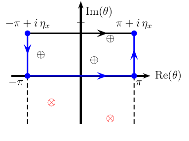
Figure 1: Contours for the integral representation (2.3) of the Appell polynomials. The original integration contour (i.e., the horizontal line connecting the points $-\pi+i\,\eta_{x}$ and $\pi+i\,\eta_{x}$) can be replaced by a new one consisting of three oriented segments (two of which will give contributions to (2.3) that cancel out due to the periodicity of the integrand). The zeroes of $g(z)$ with positive imaginary part (represented as $\oplus$) give rise to poles whose residues contribute to (2.3). The symbol $\otimes$ represents a zero of $g(z)$ with negative imaginary part.

We can now rewrite (2.3) as an integral along the segment of the real axis going from $-\pi$ to $\pi$ and a sum involving the residues of its integrand at the zeros $\theta_{k}$ of $g(e^{i\theta}/x)$ with non-negative imaginary parts. For concreteness, we will restrict ourselves to the case for which the zeroes with zero imaginary part are simple. If $\theta_{k}$ is one of these zeroes, then the integral should be replaced by its Principal Value (PV), and the corresponding residue counted with a $-1/2$ coefficient. We have, hence,

$$\frac{\pi_{n}(x)}{n!}\;=\;\frac{x^{n}}{2\pi}\,\left(\mathrm{VP}\int_{-\pi}^{\pi}\frac{e^{n(e^{i\theta}-i\theta)}}{g(e^{i\theta}/x)}\mathrm{d}\theta\;-\;2\pi i\,\sum_{k\in\mathbb{N}}\Theta\left(\mathrm{Im}(\theta_{k})\right)\,\mathrm{Res}\left(\frac{e^{n(e^{i\theta}-i\theta)}}{g(e^{i\theta}/x)}\,;\theta=\theta_{k}\right)\right)\,,$$ (2.4)

where $\Theta\;\colon\;\mathbb{R}\to\mathbb{R}$ is the step-like function defined as:

$$\Theta(x)\;=\;\begin{cases}1&\text{if $x>0$,}\\ 1/2&\text{if $x=0$,}\\ 0&\text{if $x<0$.}\end{cases}$$ (2.5)

Notice that for each zero $\zeta_{k}$ of $g(z)$, there exists an infinite number of zeroes of $g(e^{i\theta}/x)$ located at

$$\theta(\zeta_{k},j)\;=\;\mathrm{Arg}(x\zeta_{k})+2j\pi-i\log|x\zeta_{k}|\,,\quad j\in\mathbb{Z}\,.$$ (2.6)

Among these zeroes $\theta(\zeta_{k},j)$, only a single one (namely, $\theta_{k}=\theta(\zeta_{k},0)$) is contained in the strip $\mathrm{Re}(\theta)\in(-\pi,\pi]$. As $\log|x\zeta_{k}|\geq\log|xr_{0}|$, we have $-\log|x\zeta_{k}|\leq-\log|xr_{0}|<\eta_{x}$ and, hence, the imaginary parts of all the singularities of the integrand in (2.3) are strictly smaller than $\eta_{x}$ (in other words, they lie all below the integration contour chosen for (2.3)). On the other hand the zeros in (2.6) will have positive imaginary parts if, and only if, $|\zeta_{k}x|<1$, and will lie on the integration contour (i.e., the real-$\theta$ axis with $\theta\in(-\pi,\pi]$) if $|\zeta_{k}x|=1$. See figure 1 for a schematic depiction of the generic situation.

The above discussion can be summarized in the following

Theorem 2.1.

The rescaled Appell polynomials $\pi_{n}(x)=p_{n}(nx)$ (cf. (1.4)) associated to the entire function $g(z)$ [cf. (1.2)], satisfying that $g(0)\neq 0$, is equal to

$$\frac{\pi_{n}(x)}{n!}\;=\;\frac{x^{n}}{2\pi}\,\left(\mathrm{VP}\int_{-\pi}^{\pi}\frac{e^{n(e^{i\theta}-i\theta)}}{g(e^{i\theta}/x)}\,\mathrm{d}\theta\;-\;2\pi i\,\sum_{k\in\mathbb{N}}\Theta\left(\mathrm{Im}(\theta_{k})\right)\,\mathrm{Res}\left(\frac{e^{n(e^{i\theta}-i\theta)}}{g(e^{i\theta}/x)}\,;\theta=\theta_{k}\right)\right)\,,$$ (2.7)

where $\Theta$ is given by (2.5), and $\theta_{k}=\theta(\zeta_{k},0)$ corresponds to the zeroes $\zeta_{k}$ of $g(z)$ via (2.6).

Remark. The expression (2.7) for the rescaled Appell polynomial $\pi_{n}$ is exact. Even though the $\pi_{n}$ are polynomials, both terms in (2.7) are not. This expression is very useful, as one can obtain very easily its asymptotic expansion when $n\to+\infty$, as shown in section 4.

3 An integral representation using the steepest-descent path

By using the representation of the Appell polynomials provided by (2.3), it is possible to get an alternative way to write them; this one is very convenient to study their asymptotic behavior (in particular for $\pi_{n}(x)$). This new representation is obtained by deforming the integration contour in (2.3) to a new one given by curves surrounding the singularities of the integrand—whose contributions can be obtained by computing residues—, the steepest descent part $C$ of the curve defined by the condition

$$\mathrm{Im}\left(e^{i\theta}-i\theta\right)\;=\;0$$ (3.1)

($\theta=0$ is a saddle point of $\exp(e^{i\theta}-i\theta)$), and two straight segments $c_{1,2}$ parallel to the real axis in the $\theta$-complex plane (see figure 2). Notice that, owing to the $2\pi$-periodicity of the integrand in the real-$\theta$ direction, we can restrict ourselves to the strip $\mathrm{Re}(\theta)\in(-\pi,\pi]$.

If the contribution of the integration contours $c_{1,2}$ goes to zero as the imaginary parts of their points tends to $-\infty$, and if the sum of the residues picked up in the process of displacing the integration contour is finite, the integral can be extended to the full curve $C$.

The steepest descent curve $C$ passes through the origin of the complex $\theta$-plane. If we write $\theta=X+iY$ with $X\in(-\pi,\pi)$, we immediately obtain a simple implicit equation for the points of $C\setminus\{0\}$

$$X\,e^{Y}\;-\;\sin X\;=\;0\,.$$ (3.2)

Figure 2: Deformed integration contours obtained from figure 1. The real interval $\theta\in[-\pi,\pi]$ in figure 1 has been deformed to include the steepest-descent curve $C$, given by the locus of the points $\theta=X+i\,Y$ satisfying eq. (3.2) with $X\in(-\pi,\pi)$ and $Y\leq 0$. The contribution of the vertical segments at $X=\pm\pi$ vanish due to the periodicity of the integrand, and there are two ‘small’ horizontal segments $c_{1}$ and $c_{2}$ that join these vertical segments with $C$. The (negative) imaginary part of these segments $c_{1,2}$ can be made in principle as large in absolute value as desired. The hatched region represents the open set $\Omega$ (3.4). The notation for the zeroes of $g(z)$ is the same as in figure 1.

A convenient way to parametrize the curve $C$ is the following: As $C\setminus\{0\}$ is defined by the condition $\mathrm{Im}(e^{i\theta}-i\theta)=0$, for every $\tau\neq 0$ we can obtain $\theta(\tau)$ by solving the equation

$$e^{i\theta(\tau)}\;-\;i\,\theta(\tau)\;=\;1\;-\;\tau^{2}\,.$$ (3.3)

The $-\tau^{2}$ term on the r.h.s. guarantees that we are indeed dealing with the curve of steepest descent. Let us concentrate first on the solutions $\theta_{+}(\tau)$ satisfying $\mathrm{Re}(\theta_{+}(\tau))\in(0,\pi)$. Notice that from each $\theta_{+}(\tau)$ satisfying (3.3), we can obtain another solution satisfying $\mathrm{Re}(\theta_{-}(\tau))\in(-\pi,0)$ as minus its complex conjugate, i.e. $\theta_{-}(\tau)=-\overline{\theta_{+}(\tau)}$. Notice also that $\theta(0)=0$ is also a solution of (3.3).

We show now that for every $\tau>0$, there is a unique solution $\theta_{+}(\tau)\in\Omega$ to (3.3), where the region $\Omega$ is defined by the conditions

$$\Omega\;=\;\left\{\theta\in\mathbb{C}\;\colon\;\mathrm{Re}(\theta)\in(0,\pi)\wedge\mathrm{Im}(\theta)<0\right\}\,.$$ (3.4)

To this end we first notice that given a solution $\theta$ of (3.3), the number $z:=-e^{i\theta}$ satisfies

$$z\,e^{z}\;=\;-e^{\tau^{2}-1}\,.$$ (3.5)

The solutions in $z$ to this equation can be explicitly written in terms of the different branches of the Lambert function [14, 16, 15].

Given one solution $\zeta$ of (3.5), we can immediately get a solution $\theta_{\zeta}$ to (3.3) as

$$\theta_{\zeta}\;=\;i\,(1-\tau^{2}+\zeta)\,.$$ (3.6)

For $\theta_{\zeta}$ to be in $\Omega$ it is necessary that $\mathrm{Im}(\zeta)\in(-\pi,0)$. If we write $\zeta=x+iy$ with $y\in(-\pi,0)$, equation (3.5) is equivalent to

$$x \;=\;-y\,\cot y\,,$$ (3.7a)

$$e^{\tau^{2}-1} \;=\;-e^{x}\,(x\cos y\;-\;y\sin y)\,.$$ (3.7b)

For pairs $(x,y)$ satisfying (3.7a), the second equation (3.7b) tells us that $\tau(y)$ can be expressed as a continuous real function $\tau\,\colon\,(-\pi,0)\to\mathbb{R}$ such that:

$$\tau(y)\;=\;\sqrt{1-y\cot y+\log\left(\frac{y}{\sin y}\right)}\,.$$ (3.8)

This function is injective because

$$\tau^{\prime}(y)\;=\;\frac{(y-\frac{1}{2}\sin 2y)^{2}+\sin^{4}y}{2\,y\,\tau(y)\,\sin^{2}y}\;<\;0\,.$$ (3.9)

By invoking Brouwer’s Invariance of Domain theorem [17, Chapter 2], we see that the map (3.8) has a continuous inverse

$$y\;\colon\;(0,+\infty)\to(-\pi,0)\;\colon\;y\;\mapsto\;\tau(y)\,,$$ (3.10)

which is actually smooth as a consequence of the Inverse Function theorem. As we can see, for every $\tau>0$ there is a unique value $y(\tau)$ satisfying the equations (3.7). From it we compute $x(\tau)=-y(\tau)\cot y(\tau)$, and find $\theta_{+}(\tau)$. Notice that if $y\in(-\pi,0)$, we have $x=-y\cot y>-1$, hence, we see that for each $\tau>0$, the unique solution to (3.7) is contained in the open region

$$\mathcal{R}\;:=\;\left\{z\in\mathbb{C}\;\colon\;\mathrm{Re}(z)>-1\wedge\mathrm{Im}(z)\in(-\pi,0)\right\}\,.$$ (3.11)

Now we take advantage of this fact to write a closed form expression for the solution of (3.3) in terms of a suitably defined branch of the Lambert function, indeed, (3.6) can be written as

$$\theta_{+}(\tau)\;=\;i\,\left(1-\tau^{2}+W\left(-e^{\tau^{2}-1}\right)\right)\,,$$ (3.12)

where $W$ denotes the branch of the Lambert function defined by the following integral

$$W(z)\;=\;\frac{z}{2\pi i}\,\int_{\gamma}\,\frac{\xi+1}{\xi e^{\xi}-z}\,\mathrm{d}\xi\,,$$ (3.13)

and the integration contour $\gamma$, shown in figure 3(a), is the positively oriented boundary of $\mathcal{R}$ (3.11). The argument principle can be used to write (3.13) because we know that equation (3.6) has a unique solution within the region $\mathcal{R}$ delimited by $\gamma$.

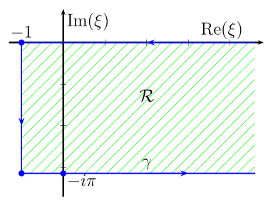
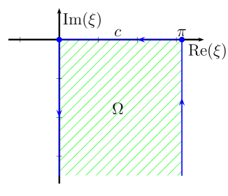
(a)	(b)

Figure 3: (a) Integration contour $\gamma$ for the integral representation of the Lambert function that we use in the paper (3.13). The contour is the boundary of the open region $\mathcal{R}$ (3.11). (b) Integration contour $c$ for the integral representation of the function $\theta_{+}(\tau)$ (3.14). In this case, this is the boundary of the open region $\Omega$ (3.4). (This region corresponds to the hatched region in figure 2.)

It is interesting to note that, for $\tau>0$, we have $W(-e^{\tau^{2}-1})=W_{-1}(-e^{\tau^{2}-1})$, where the $W_{-1}$ branch of the Lambert function is defined in [14, 16, 15].

A direct integral representation for $\theta_{+}(\tau)$—that can be derived by invoking the argument principle in the domain $\Omega$ (3.4)— is

$$\theta_{+}(\tau)\;=\;\frac{1}{2\pi}\,\int_{c}\,\frac{\xi(i\xi-\tau^{2})}{e^{i\xi}-i\xi-1+\tau^{2}}\,\mathrm{d}\xi\,,$$ (3.14)

where the contour $c$ is shown in figure 3(b) and bounds the region $\Omega$ (3.4). From this integral representation, we can immediately conclude that, given any $\tau_{0}>0$, there is an open neighborhood $U_{\tau_{0}}\in\mathbb{C}$ of the half-line $\tau>\tau_{0}$ where $\theta_{+}(\tau)$ is analytic.

We can now write a parametrization for the full steepest descent curve $C$ by defining the following function $\theta:\mathbb{R}\rightarrow\mathbb{C}$

$$\theta(\tau)\;=\;\begin{cases}\theta_{+}(\tau)&\text{if $\tau>0$,}\\ 0&\text{if $\tau=0$,}\\ -\overline{\theta_{+}(-\tau)}&\text{if $\tau<0$.}\end{cases}$$ (3.15)

It is straightforward to show that the curve $\theta(\tau)$ is smooth and satisfies $\theta^{\prime}(\tau)\neq 0$ for all $\tau\in\mathbb{R}$. In fact

$$\theta^{\prime}(\tau)\;=\;\begin{cases}\displaystyle\frac{2i\tau}{i\,\theta(\tau)-\tau^{2}}&\text{if $\tau\neq 0$,}\\[11.38109pt] \sqrt{2}&\text{if $\tau=0$.}\end{cases}$$ (3.16)

The condition $\tau^{2}=1+i\,\theta-e^{i\theta}$ defines an analytic function $\theta(\tau)$ for $\tau\in\mathbb{C}$ in a neighborhood of $\tau=0$. To see this, notice that $(1+i\,\theta-e^{i\theta})/\theta^{2}$ can be analytically extended to an entire function $h$ defined on the full complex plane satisfying $h(0)\neq 0$. This means that

$$\tau(\theta)\;=\;\theta\,\sqrt{\frac{1+i\,\theta-e^{i\theta}}{\theta^{2}}}$$ (3.17)

(where we use the branch of the square root with positive real part defined by the standard determination for the $\log$) is analytic in a neighborhood $U_{0}$ of $\theta=0$, and satisfies $\tau^{\prime}(0)\neq 0$. By taking the $\tau_{0}$ that we mentioned after (3.14) inside the open set $U_{0}$, we can actually show that the function $\theta$ (3.15) can be analytically extended to an open neighborhood of the real axis.

We have seen that $\tau(\theta)$ admits an analytic inverse $\theta(\tau)$ in a neighborhood of $\tau=0$. Its Taylor expansion around $\tau=0$ can be obtained by inverting the series expansion of $\theta(\tau)$ about $\tau=0$. However, it is interesting to mention another way to do this. The idea is to write

$$\exp(\theta(\tau))\;=\;\sum_{n=0}^{\infty}Y_{n}(i\theta^{\prime}(0),\ldots,i\theta^{(n)}(0))\,\frac{\tau^{n}}{n!}\,,$$ (3.18)

where $Y_{n}(a_{1},\ldots,a_{n})$ denotes the $n$-th complete Bell polynomial (see e.g., [13]). From this we get the following recurrence relation for the $\theta^{(k)}(0)$ ($k\geq 1$)

$$\sqrt{2} \;=\;\theta^{\prime}(0)\,,$$ (3.19a)

$$0 \;=\;Y_{n}(i\theta^{\prime}(0),\ldots,i\theta^{(n)}(0))-i\theta^{(n)}(0)\,.$$ (3.19b)

Notice that, as a consequence of the fact that the difference $Y_{n}(a_{1},\ldots,a_{n})-a_{n}$ depends only on $a_{1},\ldots,a_{n-1}$, equation (3.19b) only involves $\theta^{\prime}(0),\ldots,\theta^{(n-1)}(0)$. We give a number of terms for the Taylor expansion of $\theta(\tau)$ around $\tau=0$ in appendix A.

With the help of the parametrization of $C$ that we have introduced, we can finally write

$$\frac{x^{n}}{2\pi}\,\int_{C}\,\frac{\exp\big{(}n(e^{i\theta}-i\theta)\big{)}}{g(e^{i\theta}/x)}\,\mathrm{d}\theta\;=\;\frac{(ex)^{n}}{2\pi}\,\int_{-\infty}^{\infty}\,\frac{\theta^{\prime}(\tau)\,\exp(-n\tau^{2})}{g(e^{i\theta(\tau)}/x)}\,\mathrm{d}\tau\,.$$ (3.20)

By using the Taylor expansions that we give in appendix A, it is a simple exercise now to get as many terms of the asymptotic expansion of (3.20) as one wants in the limit $n\rightarrow+\infty$ by relying, for instance, on Watson’s lemma (as long as $x\in\mathbb{C}$ is such that no zeroes of the denominator lie on the real-$\tau$ axis). Combining these expansions with the contributions of the residues picked up in the process of deforming the integration contour to $C$, it is straightforward to get asymptotic expansions for any Appell polynomial evaluated at any value of the argument $x$. The conclusion is given by

Theorem 3.1.

The rescaled Appell polynomials $\pi_{n}(x)=p_{n}(nx)$ (cf. (1.4)) associated to the entire function $g(z)$ [cf. (1.2)], satisfying that $g(0)\neq 0$, are equal to

$$\frac{\pi_{n}(x)}{n!}\;=\;\frac{x^{n}}{2\pi}\left(e^{n}\,\mathrm{VP}\int_{-\pi}^{\pi}\frac{\theta^{\prime}(\tau)\,e^{-n\tau^{2}}}{g(e^{i\theta(\tau)}/x)}\,\mathrm{d}\tau\right.\\ \left.\;-\;2\pi i\,\sum_{k\in\mathbb{N}}\Theta\left(\psi(\theta_{k})\right)\,\mathrm{Res}\left(\frac{e^{n(e^{i\theta}-i\theta)}}{g(e^{i\theta}/x)}\,;\theta=\theta_{k}\right)\right)\,,$$ (3.21)

where $\Theta$ is given in (2.5), and the function $\psi\;\colon\;\left\{x\in\mathbb{C}\;\colon\;\mathrm{Re}(x)\in(-\pi,\pi)\right\}\to\mathbb{R}$ is defined by

$$\psi(x)\;=\;\begin{cases}\mathrm{Im}(x)-\log\left(\frac{\sin\mathrm{Re}(x)}{\mathrm{Re}(x)}\right)&\text{if $\mathrm{Re}(x)\neq 0$, }\\ \mathrm{Im}(x)&\text{if $\mathrm{Re}(x)=0$,}\end{cases}$$ (3.22)

and $\theta_{k}=\theta(\zeta_{k},0)$ correspond to the zeroes $\zeta_{k}$ of $g(z)$ through (2.6).

Remarks. 1. The definition of the function $\psi$ (3.22) is motivated by the implicit equation (3.2) satisfied by the steepest descent curve $C$. If we define $\theta=X+iY$, the points “above” or on the curve $C$ are given by the expression

$$Y\;\geq\;\begin{cases}\log\left(\frac{\sin X}{X}\right)&\text{if $X\neq 0$,}\\ 0&\text{if $X\neq 0$.}\end{cases}$$ (3.23)

2. As mentioned after Theorem 2.1, the expression (3.21) for the rescaled Appell polynomial $\pi_{n}$ is exact, and very useful to obtain its asymptotic expansion when $n\to+\infty$ (see next section).

4 Zero attractors for the rescaled Appell polynomials

The zero attractors for some Appell polynomials have been studied by a number of authors (see, for instance, [21, 9]). A landmark paper on this problem is [10], where Boyer and Goh provide a wealth of information about the zero sets of rescaled general Appell polynomials (under the condition that $g$ has, at least, one zero). The description of these sets is made easy by the application of a theorem proved by Sokal [20] that narrows down the search for the points belonging to these attractors to the determination of suitable asymptotic approximations of their integral representations (when $n\rightarrow+\infty$), and the study of their analyticity. For this purpose, the method described in the preceding sections offers a quick alternative to the one used in [10].

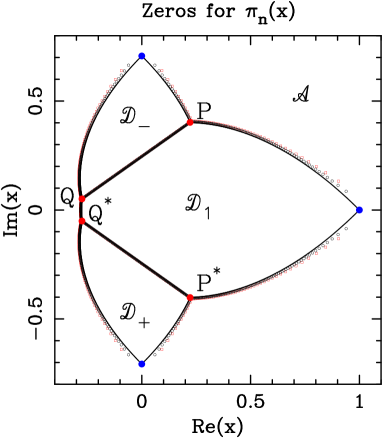
Figure 4: Zero attractor for the rescaled Appell polynomials $\pi_{n}$ with $g(x)=(x-1)(x^{2}+2)$ [10, figure 5(a)]. We show the zeros for $n=400$ (red $\Box$) and $n=1000$ (black $\circ$). The solid lines correspond to the different branches of the zero attractor in this case. Region $\mathcal{A}$ is where the integral (4.1) dominates over the residue contributions (4.3). Region $\mathcal{D}_{1}$ is where the residue of the zero at $x=1$ dominates, while regions $\mathcal{D}_{\pm}$ are where the residues of the zeros at $x=\pm i\sqrt{2}$ dominate. The blue dots (at $x=1,\pm i/\sqrt{2}$) mark the cusps corresponding to the Szegö curves due to (4.6a), and the straight segments $QP$ and $Q^{*}P^{*}$ are due to (4.6b). The red dots mark the points where three contributions collide in absolute values.

In the present setting we have to determine the asymptotic behaviors of the integral term in (2.4) and those of each of the residues. The exponent of the integral in (2.4) has a saddle point at $\theta=0$, and its asymptotic behavior (if $g(1/x)\neq 0$) is

$$\int_{-\pi}^{\pi}\,\frac{\exp\big{(}n(e^{i\theta}-i\theta)\big{)}}{g(e^{i\theta}/x)}\,\mathrm{d}\theta\;=\;\frac{e^{n}}{g(1/x)}\sqrt{\frac{2\pi}{n}}\,\left(1+O\left(\frac{1}{n}\right)\right)\,,\quad\text{as $n\rightarrow+\infty.$}$$ (4.1)

The residues in (2.4) have the form

$$\mathrm{Res}\left(\frac{\exp\big{(}n(e^{i\theta}-i\theta)\big{)}}{g(e^{i\theta}/x)}\,;\theta=\theta_{k}\right)\;=\;P_{k}(n)\,\exp\big{(}n(e^{i\theta_{k}}-i\theta_{k})\big{)}\;=\;P_{k}(n)\left(\frac{e^{\zeta_{k}x}}{\zeta_{k}x}\right)^{n}\,,$$ (4.2)

where the $P_{k}(n)$ are polynomials in $n$ with $x$-dependent coefficients. The asymptotic behavior of these residues when $n\rightarrow+\infty$ is

$$\mathrm{Res}\left(\frac{\exp\big{(}n(e^{i\theta}-i\theta)\big{)}}{g(e^{i\theta}/x)}\,;\theta=\theta_{k}\right)\;=\;c_{k}(x)\,(i\zeta_{k}x-i)^{p-1}\,n^{p-1}\,\left(\frac{e^{\zeta_{k}x}}{\zeta_{k}x}\right)^{n}\,\left(1+O\left(\frac{1}{n}\right)\right)\,,$$ (4.3)

where $p$ denotes the order of the zero $\theta_{k}$, and

$$c_{k}(x)\;=\;\frac{1}{(p-1)!}\,\lim_{\theta\rightarrow\theta_{k}}\frac{(\theta-\theta_{k})^{p}}{g(e^{i\theta}/x)}\,.$$ (4.4)

For each $x\in\mathbb{C}\setminus\{0\}$, the asymptotic behavior of $\pi_{n}(x)$ is then determined by the function

$$\Phi(x)\;=\;\max_{k\colon|\zeta_{k}x|<1}\left\{e,\left|\frac{e^{\zeta_{k}x}}{\zeta_{k}x}\right|\right\}\,.$$ (4.5)

This is the result given in [10]. In order to obtain the actual sets where the zeroes accumulate, it is necessary to find the curves defined by conditions of the type

$$\left|\frac{e^{\zeta_{k}x}}{\zeta_{k}x}\right| \;=\;e\,,\quad\text{or,}$$ (4.6a)

$$\left|\frac{e^{\zeta_{k}x}}{\zeta_{k}x}\right| \;=\;\left|\frac{e^{\zeta_{j}x}}{\zeta_{j}x}\right|\quad\text{for some indexes $k\neq j$.}$$ (4.6b)

In the first case (4.6a), we obtain rotated and rescaled Szegö curves, and in the second (4.6b), straight lines (see [10]). Notice that in the particular case of taking $g(z)=z-\zeta$ for some $\zeta\in\mathbb{C}\setminus\{0\}$, the Appell polynomials are directly related to the truncated exponential, and their zero sets are rotated and dilated Szegö curves (as dictated by the value of $\zeta$).

In figure 4, we show the zeros of the Appell polynomials associated to the choice $g(x)=(x-1)(x^{2}+2)$ [10, figure 5(a)], as well as the corresponding zero attractors in the limit $n\to+\infty$.

5 Rescaled Bernoulli polynomials

The Bernoulli polynomials $B_{n}$ are the Appell polynomials for

$$g(z)\;=\;\frac{e^{z}-1}{z}\,,$$ (5.1)

so, the integral representation for the rescaled Bernoulli polynomials $\beta_{n}(x):=B_{n}(nx)$ is given by (2.4)/(5.1). Notice that, as required, $g$ is an entire function with $g(0)=1\neq 0$.

The zeros $\zeta_{k}$ of $g(z)$ are given by $\zeta_{k}=2\pi ik$ with $k\in\mathbb{Z}\setminus\{0\}$. This means that $r_{0}=2\pi$ in this case. As $g$ is evaluated at $e^{i\theta}/x$, the zeros of $g$ correspond to the following values of $\theta$:

$$\theta_{k}\;=\;\mathrm{Arg}(kxi)-i\,\log|2\pi kx|\,,\quad\text{for $k\in\mathbb{Z}\setminus\{0\}$}\,.$$ (5.2)

In the following we prefer to work with

$$\theta_{k}^{\pm}\;:=\;\mathrm{Arg}(\pm xi)-i\,\log(2\pi k|x|)\,,\quad\text{for $k\in\mathbb{N}$.}$$ (5.3)

Notice that all zeroes $\theta_{k}^{\pm}$ are simple, and that the condition $\mathrm{Im}(\theta_{k}^{\pm})\geq 0$ implies that

$$2\pi k|x|\;\leq\;1\,.$$ (5.4)

This condition (that depends on $|x|$) will give the values of $k$ associated to the contributing zeroes. If for some $k_{\circ}\in\mathbb{N}$, $2\pi k_{\circ}|x|=1$, the corresponding zeroes $\theta_{k_{\circ}}^{\pm}$ will lie on the integration contour. The maximum value of $k\in\mathbb{N}$ contributing to the sum in (2.4) is given by

$$k_{\text{max}}(x)\;=\;\left\lfloor\frac{1}{2\pi|x|}\right\rfloor\,.$$ (5.5)

The general situation has been depicted on figure 5.

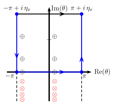
Figure 5: Generic situation for the integral representation of the rescaled Bernoulli polynomials $\beta(x)$ (2.3)/(5.1). This picture should be compared to figure 1. We have chosen $x=e^{2\pi i/3}/(6\pi)$ (with $|x|<1/(2\pi)$), and $r=\pi<r_{0}=2\pi$, so that $\eta_{x}=-\log(r|x|)=\log(6)$ and $k_{\text{max}}=3$. Notice that in this case, $\theta_{3}^{\pm}$ take real values. The zeroes of $g$ with $k\leq 7$ contributing (resp. not contributing) to the sum in (5.7) are depicted as $\oplus$ (resp. $\otimes$). They are located at $\theta_{k}^{+}=-5\pi/6-i\log(k/3)$ and $\theta_{k}^{-}=\pi/6-i\log(k/3)$.

The residues of the integrand at $\theta_{k}^{\pm}=\mathrm{Arg}(\pm xi)-i\,\log(2\pi k|x|)$, $k\in\mathbb{N}$ [cf. Eq. (5.3)] are

$$\mathrm{Res}\left(\frac{\exp\big{(}n(e^{i\theta}-i\theta)\big{)}}{g(e^{i\theta}/x)};\theta=\theta^{\pm}_{k}\right)\;=\;-\frac{i}{(2\pi kx)^{n}}\,e^{\mp in(\pi/2-2\pi kx)}\,.$$ (5.6)

The residues for $\theta_{k}^{+}$ and $\theta_{k}^{-}$ can be combined to give a cosine. We then get the

Corollary 5.1.

The rescaled Bernoulli polynomials $\beta_{n}(x)=B_{n}(nx)$ are equal to

$$\frac{\beta_{n}(x)}{n!}\;=\;\frac{x^{n}}{2\pi}\,\mathrm{PV}\!\int_{-\pi}^{\pi}\frac{e^{n(e^{i\theta}-i\theta)}}{g(e^{i\theta}/x)}\,\mathrm{d}\theta-\frac{2}{(2\pi)^{n}}\,\sum\limits_{k\in\mathbb{N}}\Theta\left(\frac{1}{2\pi|x|}-k\right)\,\frac{1}{k^{n}}\,\cos\left(n\left(\frac{\pi}{2}-2\pi kx\right)\right)\,,$$ (5.7)

where $g$ is given by (5.1), and $\Theta$, by (2.5).

Remarks. 1. Again, the expression (5.7) for the rescaled Bernoulli polynomial $\pi_{n}$ is exact for any $n\in\mathbb{N}$.

2. For any $x\in\mathbb{C}\setminus\{0\}$, the sum in (5.7) is always finite. The number of terms in that sum is given by $k_{\mathrm{max}}$ (5.5).

3. This representation is useful to obtain the asymptotic expansion of $\beta_{n}(x)$ as $n\to+\infty$ because the behavior of the cosine terms is obvious, and the asymptotics of the integral in this limit (at least, the leading term) is easy to obtain (see the remaining of this section for a general approach).

4. It is instructive to compare this expression with the Fourier series for the Bernoulli polynomials $B_{n}(x)$ [18]. As we can see, if we rescale back the variable $x\rightarrow x/n$, the upper limit $k_{\mathrm{max}}$ in the sum of (5.7) grows to $+\infty$ when $n\rightarrow+\infty$. This, together with the fact that in this limit the contribution of the integral to (5.7) is subdominant with respect to the one of the trigonometric sum, gives as a result the known Fourier representation for the Bernoulli polynomials.

We discuss now the representation of the $\beta_{n}(x)$ obtained by deforming the integration contour in (2.3) to $C$ and taking into account the residue contributions picked up in the process (as we did in section 3). See figure 6 for a depiction of this situation.

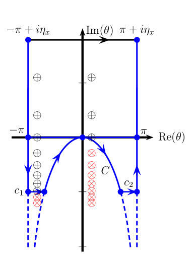
Figure 6: Deformed integration contours obtained from figure 5 (in the same way as figure 2 was obtained from figure 1). The new contour contains the steepest descent curve $C$ (3.2), as well as two small horizontal segments $c_{1,2}$. The notation is as in figures 2 and 5. The parameters $x$, $r$, and $\eta_{x}$ are chosen as in figure 5. We have shown the first $10$ zeroes $\theta_{k}^{\pm}$. The residues that contribute to (5.8) correspond to $k\leq 8$ for $\theta^{-}_{k}$, and to $k\leq 3$ for $\theta^{+}_{k}$. In this particular example, none of these zeroes falls on the integration contour.

If $x$ is not purely imaginary (i.e., if $\mathrm{Re}(x)\neq 0$), a straightforward computation gives

$$\frac{\beta_{n}(x)}{n!}\;=\;\frac{(ex)^{n}}{2\pi}\,\mathrm{VP}\int_{-\infty}^{+\infty}\,\frac{e^{-n\tau^{2}}\theta^{\prime}(\tau)}{g(e^{i\theta(\tau)}/x)}\mathrm{d}\tau-\frac{1}{(2\pi)^{n}}\,\sum_{k\in\mathbb{N}}\Theta\left(\frac{\mathrm{Arg}(ix)}{2\pi\mathrm{Im}(ix)}-k\right)\,\frac{e^{2k\pi inx}}{(ik)^{n}}\\ -\frac{1}{(2\pi)^{n}}\,\sum_{k\in\mathbb{N}}\Theta\left(\frac{\mathrm{Arg}(-ix)}{2\pi\mathrm{Im}(-ix)}-k\right)\,\frac{e^{-2k\pi inx}}{(-ik)^{n}}\,,\qquad\qquad$$ (5.8)

where $g$ is given by (5.1) and $\Theta$, by (2.5). Notice that the upper limits in the sums of the r.h.s. of (5.8) are finite in this case ($\mathrm{Re}(x)\neq 0$), but may be different from each other for generic choices of $x\in\mathbb{C}\setminus\{0\}$. (See figure 6.)

Remark. The argument of the function $\Theta$ in (5.8) comes directly from the generic condition (3.23) for a zero $\theta_{k}$ to be “above” or on the steepest descent curve $C$ (3.2), and the particular form for these zeros for the Bernoulli case (5.3).

For $x=iq$ with $q>0$, we find

$$\frac{\beta_{n}(x)}{n!}\;=\;\frac{(ex)^{n}}{2\pi}\,\mathrm{VP}\int_{-\infty}^{+\infty}\frac{e^{-n\tau^{2}}\theta^{\prime}(\tau)}{g(e^{i\theta(\tau)}/x)}\,\mathrm{d}\tau-\frac{1}{(2\pi i)^{n}}\,\mathrm{Li}_{n}\big{(}e^{2\pi inx}\big{)}\\ -\frac{1}{(2\pi)^{n}}\,\sum_{k\in\mathbb{N}}\Theta\left(\frac{1}{2\pi\mathrm{Im}(x)}-k\right)\,\frac{e^{-2\pi iknx}}{(-ik)^{n}}\,,$$ (5.9)

where $\mathrm{Li}_{n}$ denotes the polylogarithm, and $\Theta$ is given by (2.5). The expression for $x=iq$ for $q<0$ is obtained from the previous one by complex conjugation.

Several comments are in order now

1) Whenever the upper limits in the sums on the r.h.s. of (5.8) are smaller than one, the $\beta_{n}(x)/n!$ are given exactly by integral on the r.h.s. of (5.8), which is written in a form that makes it specially easy to study its asymptotic behavior when $n\rightarrow+\infty$.

The first two terms of the asymptotic expansion of the integral that appears on the r.h.s. of (5.8) in the limit $n\rightarrow+\infty$ can be obtained by using the expressions given in appendix A. In the case $\exp(1/x)-1\neq 0$, we have

$$\frac{(ex)^{n}}{2\pi}\,\mathrm{VP}\int_{-\infty}^{+\infty}\frac{e^{-n\tau^{2}}\theta^{\prime}(\tau)}{g(e^{i\theta(\tau)}/x)}\,\mathrm{d}\tau\;=\;\frac{e^{n}x^{n-1}}{(e^{1/x}-1)\,\sqrt{2\pi n}}\\ \times\left(1-\frac{x^{2}+e^{2/x}(6-12x+x^{2})-2e^{1/x}(x^{2}-6x-3)}{12x^{2}(e^{1/x}-1)^{2}}\,\frac{1}{n}+O\left(\frac{1}{n^{2}}\right)\right)\,,$$ (5.10)

whereas, for $1/x=2\pi im$ with $m\in\mathbb{Z}\setminus\{0\}$, the asymptotic expansion when $n\to+\infty$ of the integral on the r.h.s. of (5.9) is

$$\frac{(ex)^{n}}{2\pi}\, \mathrm{VP}\int_{-\infty}^{+\infty}\frac{e^{-n\tau^{2}}\theta^{\prime}(\tau)}{g(e^{i\theta(\tau)}/x)}\,\mathrm{d}\tau$$

$$\;=\;\frac{(ex)^{n}}{2\sqrt{2\pi n}}\,\left(\frac{2}{3}-\frac{1}{x}+\left(\frac{1}{270}+\frac{1}{12x}-\frac{1}{6x^{2}}\right)\,\frac{1}{n}+O\left(\frac{1}{n^{2}}\right)\right)$$ (5.11a)

$$\;=\;\left(\frac{e}{2\pi im}\right)^{n}\,\frac{1}{2\sqrt{2\pi n}}\,\left(\frac{2}{3}-2\pi im+\left(\frac{1}{270}+\frac{m\pi i}{6}+\frac{2m^{2}\pi^{2}}{3}\right)\,\frac{1}{n}+O\left(\frac{1}{n^{2}}\right)\right)\,.$$ (5.11b)

2) The contributions of the curves $c_{1,2}$ (see figure 2) can be easily seen to go to zero as they are displaced in the direction of the negative imaginary axis. This is a consequence of the rapid fall off of the term $\exp(n(e^{i\theta}-i\theta))$. In the case $\mathrm{Re}(x)\neq 0$, only finite sums are involved, so the convergence of the integral in equation (5.8) is guaranteed. If $\mathrm{Re}(x)=0$, some care is needed, as we have to deal with an infinite number of contributions from singularities located at points with real parts equal to $\pm\pi$. In this case, the sum will be proportional to the polylogarithm $\mathrm{Li}_{n}(e^{\pm 2\pi inx})$, which is finite in general. The best way to proceed is to restrict oneself to contours $c_{1,2}$ with imaginary part equal to $-\log\big{(}(2k+1)\pi|x|\big{)}$ and bound the integrals on those specific contours.

3) As far as the asymptotics of the $\beta_{n}(x)$ in the limit $n\rightarrow+\infty$ is concerned, the previous representations tell us the relative contributions of the different terms. Notice, for instance, that the denominators in the sums on the r.h.s. of (5.8) exponentially suppress the contributions of the terms with $k>1$ (if present). The asymptotic behavior of the integral term in (5.8) is controlled by an exponential factor $(ex)^{n}$. If this factor turns out to outweigh the contributions of the $k=1$ terms of the these sums, all the terms in the asymptotic expansion of the integral will dominate over the ones coming from the sums.

Appendix A Parametrization of the steepest descent curve $\bm{C}$

By solving the recurrence relation (3.19), we can easily get as many terms of the Taylor expansion of $\theta(\tau)$ around $\tau=0$ as we need. The terms up to $O(\tau^{9})$ are

$$\theta(\tau)\;=\;\sqrt{2}\tau-\frac{i\tau^{2}}{3}-\frac{\tau^{3}}{9\sqrt{2}}+\frac{2i\tau^{4}}{135}+\frac{\tau^{5}}{540\sqrt{2}}+\frac{4i\tau^{6}}{8505}+\frac{139\tau^{7}}{340200\sqrt{2}}-\frac{2i\tau^{8}}{25515}+O(\tau^{9})\,.$$ (A.1)

For an entire function $g$ such that $g(0)\neq 0$ and $g(1/x)\neq 0$, we get to $O(\tau^{3})$

$$\frac{\theta^{\prime}(\tau)}{g\big{(}\exp(i\theta(\tau))/x\big{)}}\;=\;\frac{\sqrt{2}}{g_{0}(x)}-\frac{2(xg_{0}(x)+3g_{1}(x))}{3xg_{0}^{2}(x)}\tau\\ -\frac{x^{2}g_{0}^{2}(x)+12g_{1}^{2}(x)-6g_{0}(x)g_{2}(x)}{3\sqrt{2}x^{2}g_{0}^{3}(x)}\tau^{2}+O(\tau^{3})\,,\qquad$$ (A.2)

where we use the shorthand notation $\displaystyle g_{n}(x):=g^{(n)}(1/x)$.

If $g(1/x)\neq 0$ and $x\neq 0$ is such that no singularities of the integrand lie on the integration contour $C$, the first terms of the asymptotic expansion for (3.20) in the limit $n\rightarrow+\infty$ are

$$\frac{x^{n}}{2\pi}\,\int_{C}\frac{\exp\big{(}n(e^{i\theta}-i\theta)\big{)}}{g(e^{i\theta}/x)}\,\mathrm{d}\theta\;=\;\frac{(ex)^{n}}{\sqrt{2\pi n}}\,\left(\frac{1}{g_{0}(x)}\right.\\ -\left.\left(\frac{1}{12g_{0}(x)}+\frac{g_{1}^{2}(x)}{x^{2}g_{0}^{3}(x)}-\frac{g_{2}(x)}{2x^{2}g_{0}^{2}(x)}\right)\,\frac{1}{n}+O\left(\frac{1}{n^{2}}\right)\right)\,.$$ (A.3)

If $x$ is such that some of the singularities (simple poles) of the integrand lie on the integration contour $C$ away from $\theta=0$, a straightforward argument leads to the conclusion that the preceding expression (A.3) remains valid for the PV of the integral appearing on its l.h.s.

Finally, if $x$ is such that $\theta=0$ is a simple pole of the integrand, we have

$$\frac{x^{n}}{2\pi}\,\mathrm{PV}\int_{C}\frac{\exp\big{(}n(e^{i\theta}-i\theta)\big{)}}{g(e^{i\theta}/x)}\,\mathrm{d}\theta\;=\;\frac{(ex)^{n}}{2\sqrt{2\pi n}}\;\left(-\frac{4xg_{1}(x)+3g_{2}(x)}{3g_{1}^{2}(x)}\right.\\ +\frac{92x^{3}g_{1}^{3}(x)+135g_{2}^{3}(x)-180g_{1}(x)g_{2}(x)g_{3}(x)+45g_{1}^{2}(x)\big{(}x^{2}g_{2}(x)+g_{4}(x)\big{)}}{540x^{2}g_{1}^{4}(x)}\,\frac{1}{n}\\ +\left.O\left(\frac{1}{n^{2}}\right)\right)\,.\qquad\qquad\qquad\qquad$$ (A.4)

References

- [1] M. Anshelevich, Appell polynomials and their relatives. Int. Math. Res. Not. 65 (2004) 3469–3531, arXiv:math/0311043.
- [2] M. Anshelevich, Appell polynomials and their relatives. II. Boolean theory. Indiana Univ. Math. J. 58 (2009) 929–968, arXiv:0712.4185.
- [3] M. Anshelevich, Appell polynomials and their relatives. III. Conditionally free theory. llinois J. Math. 53 (2009), 39–66, arXiv:0803.4279.
- [4] P.E. Appell, Sur une classe the polynômes, Ann. Sci. École Norm. Sup. 9 (1880) 119–144.
- [5] C.M. Bender and S.A. Orszag, Advanced Mathematical Methods for Scientists and Engineers I (Springer Verlag, 1999).
- [6] S. Beraha, J. Kahane and N.J. Weiss, Limits of zeroes of recursively defined polynomials, Proc. Nat. Acad. Sci. USA 72 (1975) 4209.
- [7] S. Beraha, J. Kahane and N.J. Weiss, Limits of zeroes of recursively defined families of polynomials, in Studies in Foundations and Combinatorics (Advances in Mathematics Supplementary Studies, Vol. 1), ed. G.-C. Rota, pp. 213-232 (Academic Press, New York, 1978).
- [8] S. Beraha, J. Kahane and N.J. Weiss, Limits of chromatic zeros of some families of maps, J. Combin. Theory Ser. B 28 (1980) 52-65.
- [9] R.P. Boyer and W.M.Y. Goh, On the Zero Attractor of the Euler Polynomials, Adv. Appl. Math. 38 (2007), 97–132.
- [10] R.P. Boyer and W.M.Y. Goh, Appell Polynomials and Their Zero Attractors, Gems in Experimental Mathematics, Contemp. Math. 517 (2010) 69–96 (AMS, Providence RI, 2010), arXiv:0809.1266.
- [11] T. Burić and N. Elezović, Bernoulli polynomials and asymptotic expansions of the quotient of gamma functions, J. Comput. Appl. Math. 235 (2011) 3315 -3331.
- [12] T. Burić, N. Elezović and L. Vukšić, Appell Polynomials and Asymptotic Expansions, Mediterr. J. Math. 13 (2016) 899 -912.
- [13] L. Comtet, Advanced Combinatorics (D. Reidel Publishing Company, Dordrecht, Holland, 1974).
- [14] R.M. Corless, G.H. Gonnet, D.E.G. Hare, D.J. Jeffrey, and D.E. Knuth, On the Lambert function, Adv. Comput. Math. 5 (1996) 329–359.
- [15] R.M. Corless, D.J. Jeffrey, and D.E. Knuth, A sequence of series for the Lambert function. Proceedings of the 1997 International Symposium on Symbolic and Algebraic Computation, (Kihei, HI), pp. 197–204 (ACM, New York, 1997).
- [16] D.J. Jeffrery, D.E.G. Hare, and R.M. Corless, Unwinding the branches of the Lambert function, Math. Sci. 21 (1996) 1–7.
- [17] A. Hatcher, Algebraic Topology (Cambridge University Press, Cambridge, 2002).
- [18] J.L. López and N.M. Temme, Large degree asymptotics of generalized Bernoulli and Euler polynomials, J. Math. Anal. Appl. 363 (2010) 197–208.
- [19] S. Roman, The umbral calculus (Dover Publications Inc., Mineola N.Y., 2005).
- [20] A.D. Sokal, Chromatic roots are dense in the whole complex plane, Combin. Probab. Comput. 13 (2004) 221–261, arXiv:cond-mat/0012369.
- [21] G. Szegö, Über eine Eigenschaft der Exponentialreihe, Sitzungsber. Berl. Math. Ges., 23 (1924), 50–64.
- [22] C.N. Yang and T.D. Lee, Statistical Theory of Equations of State and Phase Transitions. I. Theory of Condensation, Phys. Rev. 87 (1952) 404–409.