Suppressing cosmic variance with paired-and-fixed cosmological simulations: average properties and covariances of dark matter clustering statistics

Abstract

Making cosmological inferences from the observed galaxy clustering requires accurate predictions for the mean clustering statistics and their covariances. Those are affected by cosmic variance – the statistical noise due to the finite number of harmonics. The cosmic variance can be suppressed by fixing the amplitudes of the harmonics instead of drawing them from a Gaussian distribution predicted by the inflation models. Initial realisations also can be generated in pairs with $180^{\circ}$ flipped phases to further reduce the variance. Here, we compare the consequences of using paired-and-fixed vs Gaussian initial conditions on the average dark matter clustering and covariance matrices predicted from $N$-body simulations. As in previous studies, we find no measurable differences between paired-and-fixed and Gaussian simulations for the average density distribution function, power spectrum and bispectrum. Yet, the covariances from paired-and-fixed simulations are suppressed in a complicated scale- and redshift-dependent way. The situation is particularly problematic on the scales of Baryon Acoustic Oscillations where the covariance matrix of the power spectrum is lower by only $\sim 20\%$ compared to the Gaussian realisations, implying that there is not much of a reduction of the cosmic variance. The non-trivial suppression, combined with the fact that paired-and-fixed covariances are noisier than from Gaussian simulations, suggests that there is no path towards obtaining accurate covariance matrices from paired-and-fixed simulations. Because the covariances are crucial for the observational estimates of galaxy clustering statistics and cosmological parameters, paired-and-fixed simulations, though useful for some applications, cannot be used for the production of mock galaxy catalogs.

1 Introduction

Large galaxy redshift surveys yield vital knowledge on numerous properties of the large-scale structure of the universe, many of the key cosmological parameters and the nature of dark matter. While the signal—whatever statistics are used—is measured using observational data, its uncertainties and errors are typically obtained by theoretical modelling and understanding the phenomena involved (e.g., Mandelbaum et al., 2013; Rodríguez-Torres et al., 2016; MacCrann et al., 2018; van Uitert et al., 2018). Cosmological simulations play a crucial role in the process of estimating the errors.

More specifically, cosmological simulations generate two types of results: i) the average statistics – such as the power spectrum, correlation function, or weak-lensing signal – for the adopted cosmological parameters, and ii) covariance matrices, i.e., the correlation of the measured statistics at different bins. For example, this can be the correlation of power spectra values at different wavenumbers or the correlations of values of the correlation function at different radii.

The average properties of clustering statistics are important on their own. They provide a preliminary test of whether a given cosmological model can reproduce the observations. If it clearly cannot, there is no need to perform a detailed analysis constraining the particular cosmological model. Average properties themselves are difficult to estimate. This requires a procedure to connect dark matter with galaxies, which is one of the fundamental problems of modern cosmology (e.g., Somerville & Davé, 2015; Wechsler & Tinker, 2018). There are different methods and techniques for how to do this in the context of large cosmological surveys (e.g., Somerville & Primack, 1999; Conroy et al., 2006; Trujillo-Gomez et al., 2011; Rodríguez-Torres et al., 2016; Monaco, 2016).

However, once we know how to estimate the average statistics, we face an even more difficult challenge: we need to produce many realisations of the statistics to estimate the covariance matrix which describes the errors of the observations. The number of realisations depends on the particular statistics that are used, but typically one needs to run many thousands of simulations to obtain accurate estimates of error bars and covariance matrices (e.g. see Klypin & Prada, 2018, and references therein). This puts significant stress on theoretical predictions, and practically discards some computational methods such as direct hydro-dynamical simulations of galaxy formation or high-resolution $N$-body simulations. They will be too expensive to run for thousands of realisations.

In the last few years, new techniques have been developed to address the need for massive production of mock galaxy samples. These include $N$-body codes such as COLA (Tassev et al., 2015; Koda et al., 2016) and GLAM (Klypin & Prada, 2018) that are very fast and have sufficient resolution for some observational statistics. There are also approximate methods that lack predictive power, but can be used for estimates of covariances (Kitaura et al., 2016; Monaco, 2016; Baumgarten & Chuang, 2018; Lippich et al., 2019).

A different approach has been recently proposed by Angulo & Pontzen (2016). In order to reduce the scatter between different realisations, i.e., the effects of cosmic variance, they suggest fixing the amplitudes of the Fourier harmonics. Instead of having purely Gaussian initial conditions, as typically predicted by inflation models (Mukhanov et al., 1992; Bartolo et al., 2004), the amplitudes of the harmonics are fixed to have the same magnitude as the ensemble average power spectrum. In addition, the realisations can be run in pairs with the phases flipped by $180\,^{\circ}$ to further reduce the noise (Pontzen et al., 2016). The real fluctuations which originated during inflation should not have fixed amplitudes, meaning that the paired-and-fixed method is a trick to reduce the noise. However, this method can be quite useful. Its success comes from the fact that in the linear regime the fixed-amplitude density perturbation field $\delta\rho({\mn@boldsymbol{x}},t)$ has a Gaussian distribution with the correlation function being the same as for normal perturbations, i.e., $\langle\delta\rho({\mn@boldsymbol{x}},t)\delta\rho({\mn@boldsymbol{x}}+{\mn@boldsymbol{x}}^{\prime},t)\rangle$. This implies, for example, that it has the same statistics for the high-$\sigma$ peaks responsible for the formation of the most massive halos. It has the same mixture of long and short wavelengths (as manifested by the power spectrum), and thus the same sequence of growing non-linear structures.

The paired-and-fixed method has been implemented and studied in a number of publications. Angulo & Pontzen (2016) found that the dark matter power spectrum from a single pair of fixed simulations reproduces the average power spectrum nearly as well as an ensemble of 300 standard Gaussian simulations at $z=1$, even on deeply non-linear scales, $k\approx 1\mbox{$\,h$Mpc${}^{-1}$}$. Similarly good agreement was found for the mass function, bispectrum and correlation function. However, because only one pair of fixed simulations was used for the comparison, the residual r.m.s. errors of the statistics from the paired-and-fixed method, relative to the standard method, were noisy. For example, the r.m.s. deviations for the power spectrum were very small on large scales ($k\mbox{${\,\hbox{\hbox{$<$}\kern-8.00003pt\lower 4.30554pt\hbox{$\sim$}}\,}$}0.02\mbox{$\,h$Mpc${}^{-1}$}$), but they became increasingly noisy on smaller scales. On the other hand, the r.m.s. deviations of the mass function did not become smaller by using the paired-and-fixed simulations. The paired-and-fixed method thus appears to be a powerful tool for quickly achieving small r.m.s. errors for some statistics, but more extensive analyses of the r.m.s. residuals and covariances are clearly needed. More realisations of paired-and-fixed simulations could be used to examine the average r.m.s. errors, and comparison with different simulation codes could confirm the robustness of the method.

Villaescusa-Navarro et al. (2018) used 100 realisations of both Gaussian and paired-and-fixed simulations using the Gadget code with $512^{3}$ particles in a 1 $h^{-1}$Gpc  box. Because of the high force resolution of the Gadget simulations, the analysis of the power spectrum was done up to $k\sim 1\mbox{$\,h$Mpc${}^{-1}$}$. As in Angulo & Pontzen (2016), they also found a dramatic suppression in the scatter of the matter power spectrum at long wavelengths: a factor of $10^{3}$ in the r.m.s. at $k=0.01\mbox{$\,h$Mpc${}^{-1}$}$. At smaller scales, the r.m.s. tends towards the same result as for Gaussian simulations, but upon closer inspection the r.m.s. errors for the matter power spectrum are systematically smaller. Villaescusa-Navarro et al. (2018) also studied the density probability distribution function (PDF) for the relatively large cell size of $\sim 8\,\mbox{$h^{-1}$Mpc}$, which probed the density field up to modest over-densities, $\delta\rho/\rho<50$. Overall, their main conclusion was that the scatter (cosmic variance) can be strongly suppressed for the power spectrum on large scales, but not as much for the mass function or the power spectrum on small scales. The relatively small number of realisations translated into noisy r.m.s. values and did not allow for an analysis of the covariances.

One of the main goals of large-volume cosmological simulations is to estimate the scatter and covariances of statistics observed by large galaxy surveys. In that respect the main advantage of the paired-and-fixed simulations—reduced scatter—begins to appear problematic. Indeed, the realisation-to-realisation scatter, such as the scatter in the power spectrum or bispectrum at a fixed wavenumber, is simply the diagonal component of the covariance matrix. If it is reduced, then the covariance matrix will be incorrect. To date the scatter has been measured with large errors, and there has been no exploration of the effect on full covariance matrices.

With 400 realisations of a $1\,\mbox{$h^{-1}$Gpc}$ simulation box Chuang et al. (2018) had enough data to study the scatter of the power spectrum in more detail than Villaescusa-Navarro et al. (2018). They found that relative to the Gaussian simulations, the scatter in paired-and-fixed simulations was scale-dependent and approaching unity at $k\mbox{${\,\hbox{\hbox{$>$}\kern-8.00003pt\lower 4.30554pt\hbox{$\sim$}}\,}$}0.2\mbox{$\,h$Mpc${}^{-1}$}$ and $z=1$. However, at these small scales the r.m.s. estimates were too noisy to determine whether the ratio of Gaussian to paired-and-fixed r.m.s. was indeed constant. Chuang et al. (2018) also argued that because the non-diagonal covariance matrix scales as $1/V$, where $V$ is the simulation volume, the full covariance matrix should be smaller compared to the Gaussian simulations by a factor of $1/V$. This would imply that a single pair of fixed simulations is effectively measuring the covariance matrix of a large ensemble of Gaussian simulations. However, this reasoning was not substantiated by an analysis of the simulations. It also contradicts the authors’ own results which show that the diagonal components of the covariance matrix depend on the wavenumber $k$, and thus cannot simply be re-scaled by $1/V$ to obtain the same covariance matrix as an ensemble of Gaussian simulations. The results presented in this paper contradict the Chuang et al. (2018) claim that paired-and-fixed covariance matrices can be scaled with the simulation volume.

The main goal of our paper is to study in detail, using thousands of $N$-body simulations, the r.m.s. scatter and covariance matrices measured from paired-and-fixed simulations. How do they depend on scale and redshift? Is this dependence a simple one which can be rescaled to recover the covariances of the true Gaussian simulations? To answer these questions we made a very large number ($\sim 4000$) of realisations with Gaussian and paired-and-fixed initial conditions using the GLAM code. This allows us to study the diagonal and off-diagonal covariances of the power spectrum and the diagonal covariances of the bispectrum.

Section 2 provides some background on paired-and-fixed, as well as Gaussian, initial conditions. In Section 3 we give the details of our GLAM simulations. The average power spectrum and density distribution function results are given in Section 4. In Section 5 we discuss the results on the covariance matrix of the power spectrum. The impact on the bispectrum and its scatter is presented in Section 6. We end with a discussion of our main conclusions in Section 7.

2 Paired-and-fixed simulations

The adopted computational domain is a cubic box of size $L$ and volume $V=L^{3}$. In this case the fundamental mode $k_{f}=2\pi/L$ of this domain defines the discreteness in Fourier space: ${\mn@boldsymbol{k}}=(k_{x},k_{y},k_{z})=(i,j,k)k_{f}$, where $(i,j,k)$ are integer numbers. The density contrast in the domain can be expanded into the Fourier series as follows

$$\delta({\mn@boldsymbol{x}},t)\equiv\frac{\delta\rho}{\rho}=\sum_{{\mn@boldsymbol{k}}}\delta_{{\mn@boldsymbol{k}}}e^{i{\mn@boldsymbol{k}}{\mn@boldsymbol{x}}}.$$ (1)

In the linear regime the amplitudes of the harmonics $\delta_{{\mn@boldsymbol{k}}}$ are uncorrelated random numbers that must obey two conditions. First, because $\delta({\mn@boldsymbol{x}})$ are real numbers, $\delta_{-{\mn@boldsymbol{k}}}=\delta_{{\mn@boldsymbol{k}}}^{*}$. Second, in the linear regime the curl of the velocity field must be equal to zero. The condition that $\delta_{-{\mn@boldsymbol{k}}}=\delta_{{\mn@boldsymbol{k}}}^{*}$ implies that only half of the harmonics in Fourier space are independent. We can explicitly use this by writing the summation given in eq. (1) over half of the Fourier space (Binney & Tremaine, 2008, eq. 9.10):

$$\delta({\mn@boldsymbol{x}},t) = {\sum}^{\prime}\delta_{{\mn@boldsymbol{k}}}e^{i{\mn@boldsymbol{k}}{\mn@boldsymbol{x}}}+\delta_{-{\mn@boldsymbol{k}}}e^{-i{\mn@boldsymbol{k}}{\mn@boldsymbol{x}}}$$ (2)

$$= \alpha{\sum}^{\prime}\sqrt{P(|{\mn@boldsymbol{k}}|)}[A\cos({\mn@boldsymbol{k}}{\mn@boldsymbol{x}})+B\sin({\mn@boldsymbol{k}}{\mn@boldsymbol{x}})]$$ (3)

$$= \alpha{\sum}^{\prime}\sqrt{P(|{\mn@boldsymbol{k}}|)}C\cos({\mn@boldsymbol{k}}{\mn@boldsymbol{x}}+\phi).$$ (4)

Here $\alpha$ is a normalization factor, $P(|{\mn@boldsymbol{k}}|)$ is the initial power spectrum for a given cosmology, and the parameters $A$ and $B$ are random numbers following a Gaussian distribution with zero mean and dispersion unity. In eq. (4) the parameter $C$ is a random number following a chi distribution with two degrees of freedom, $C=\sqrt{A^{2}+B^{2}}$, which is also known as the Rayleigh distribution. The parameter $\phi$ is a random number that is uniformly distributed between 0 and $\pi$.

Both forms for the density spectrum, eq. (3) and eq. (4), are widely used for setting up the initial conditions. We prefer to use eq. (3) because it is easy to implement for real-to-real FFT routines, which require only half as much memory to be allocated compared to complex-to-complex FFTs. Otherwise they are mathematically identical.

In order to generate paired initial conditions, one simply adds $\pi$ to the phase $\phi$ in eq. (4) or changes the signs of $A$ and $B$ in eq. (3). In both cases the sum of paired realisations gives $\delta({\mn@boldsymbol{x}})+\delta_{\rm paired}({\mn@boldsymbol{x}})=0$. This setup with the Gaussian or Rayleigh random numbers sets the initial conditions for perturbations generated during inflation.

For fixed amplitude simulations one assumes that $A$ and $B$ are random numbers, but their distribution is peculiar: they are either one or minus one, i.e. $A,B=(-1,1)$. By design, the sum of squares of the amplitudes of the harmonics for each narrow bin $(k,k+\Delta k)$ in Fourier space returns exactly the input power spectrum $P(k)$. This is not the case for truly Gaussian initial conditions where the power spectrum of a given realisation has the following r.m.s. deviations:

$$\frac{\Delta P}{P}=\left(\frac{2}{N_{h}}\right)^{1/2},\quad N_{h}=\frac{4\pi k^{2}\Delta k}{k_{f}^{3}},$$ (5)

where $k_{f}$ and $N_{h}$ are the fundamental harmonic and the number of harmonics, respectively.

In spite of the fact that fixed amplitude initial conditions do not have the correct distribution of the amplitudes in phase space, its density field $\delta({\mn@boldsymbol{x}})$ has the same distribution as in the purely Gaussian initial conditions: it is a Gaussian field with the same correlation function by virtue of the central limit theorem. The sum of random variables with the same distribution—in our case the $A$ and $B$ variables in eq. (3)—has a Gaussian distribution.

In the same way, one expects that any statistic that is a convolution of many Fourier components will have the same average property in both fixed and Gaussian simulations. For example, the correlation function is a convolution of the power spectrum:

$$\xi(r)=\frac{1}{2\pi^{2}}\int_{0}^{\infty}k^{2}dkP(k)\frac{sin(kr)}{kr}.$$ (6)

Thus, it must be the same for fixed and Gaussian simulations. The same holds for the mass function.

However, one expects differences for the second-order statistics: the r.m.s. scatter and covariance matrices. Indeed, there is no scatter of the power spectrum or the correlation function for fixed simulations. This likely means that other statistics, such the r.m.s. of the bispectrum, may also be affected.

The situation becomes more complicated in the non-linear regime. The fixed amplitude perturbations still produce random fields: the combination of “+” and “–” signs for the parameters $A$ and $B$ varies from realisation to realisation. Non-linear interactions affect these random fields in a complicated way. As we will see later, non-linearities typically amplify the random nature of the perturbations resulting in a substantial increase of the scatter and covariances.

Considering these potential effects and the existing results in the literature, in this paper we have two main goals: i) to understand the non-linear effects and accuracy of paired-and-fixed simulations by studying the power spectrum and high-mass end of the density distribution function, and ii) to examine the scatter and covariance matrices of the power spectrum and bispectrum from paired-and-fixed simulations.

Table 1: Numerical parameters of the GLAM simulations used in this work. The columns give the simulation identifier, the size $L$ of the simulated box in $h^{-1}\,{\rm Mpc}$, the number of particles $\mbox{$N_{\rm p}$}^{3}$, the mass per particle $m_{p}$ in units of $h^{-1}\,M_{\odot}$, the mesh size $\mbox{$N_{\rm g}$}^{3}$, the gravitational softening length $\epsilon$ in units of $h^{-1}\,{\rm Mpc}$, the number of realisations $N_{r}$ and the total volume in $h^{-1}\,{\rm Gpc}^{3}$.

Simulation	$L^{3}$	$\mbox{$N_{\rm p}$}^{3}$	$m_{p}$	$\mbox{$N_{\rm g}$}^{3}$	$\epsilon$	$N_{r}$	$V_{\rm tot}$	Initial conditions
1GpcGauss	10003	10003	$8.5\times 10^{10}$	20003	0.50	1200	1200	Gaussian fluctuations
1GpcFixed	10003	10003	$8.5\times 10^{10}$	20003	0.50	600	600	Fixed amplitude fluctuations
1GpcPairedFixed	10003	10003	$8.5\times 10^{10}$	20003	0.50	600	600	Paired simulations for 1GpcFixed
3GpcGauss	30003	10003	$2.3\times 10^{12}$	20003	1.50	1300	35000	Gaussian fluctuations
3GpcFixed	30003	10003	$2.3\times 10^{12}$	20003	1.50	25	675	Fixed amplitude fluctuations
3GpcPairedFixed	30003	10003	$2.3\times 10^{12}$	20003	1.50	25	675	Paired simulations for 3GpcFixed
C1.2	12003	20003	$1.8\times 10^{10}$	50003	0.24	22	38	Gaussian fluctuations

3 Simulations

We use the Parallel Particle-Mesh $N$-body code GLAM (Klypin & Prada, 2018) that provides us with a tool to quickly generate a large number of $N$-body cosmological simulations with reasonable speed and acceptable numerical resolution. For a particular cosmological model and initial conditions, GLAM generates the density field, including peculiar velocities. The code uses a regularly spaced three-dimensional mesh of size $N_{\rm g}^{3}$ that covers the cubic domain $L^{3}$ of a simulation box using $N_{\rm p}^{3}$ particles. The size of a cell $\epsilon=L/N_{\rm g}$ and the mass of each particle $m_{\rm p}$ define the force and mass resolutions, respectively.

The number of time-steps $N_{\rm s}$ is proportional to the computational cost of the simulation. This is why reducing the number of steps is important for producing a large set of realisations. White et al. (2014) and Koda et al. (2016) use just $\sim 10$ time-steps for their QPM and COLA simulations. Feng et al. (2016) and Izard et al. (2015) advocate using $\mbox{$N_{\rm s}$}\approx 40$ steps for Fast-PM and ICE-COLA.

Because our main goal is to produce simulations requiring minimal corrections to the local density and peculiar velocities, we use $\mbox{$N_{\rm s}$}=136$ time-steps in our GLAM simulations. This number of steps also removes the need to split particle displacements into quasi-linear ones and the deviations from quasi-linear predictions. In this way we greatly reduce the complexity of the code and increase its speed, while also substantially reducing the memory requirements. See Klypin & Prada (2018) for more details.

We use a very large number of GLAM simulations—about 4,000—to study different aspects of dark matter clustering statistics in the flat $\Lambda$CDM Planck cosmology with parameters $\sigma_{8}=0.828$, $\Omega_{\Lambda}=0.693$, $\Omega_{m}=0.307$, $\Omega_{b}=0.048$ and $h=0.678$. The numerical parameters of our simulations are presented in Table 1. All of the simulations were started at an initial redshift $z_{\rm init}=100$ using the Zeldovich approximation.

When generating the initial conditions for fixed amplitude simulations, we use the same code that generates true Gaussian simulations. However, the amplitudes of the Fourier harmonics are replaced by either one or minus one depending on the sign of the random Gaussian number used in normal simulations. To generate a paired realisation, we flip the phases by $180\,^{\circ}$.

The analysis of paired and fixed simulations is done by first averaging the results within each pair and then getting the statistics of the averages. This procedure reduces the scatter by $\sqrt{2}$ even for completely independent realisations. In order to compensate for this effect we scale up the scatter by $\sqrt{2}$, which effectively provides the scatter per realisation.

4 Power Spectrum and Density Distribution Function

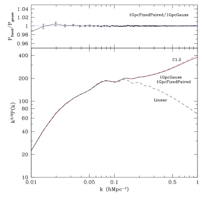
Figure 1: Bottom panel: Power spectra of dark matter at redshift $z=0$ scaled by the factor $k^{3/2}$ to highlight the BAO region at $k=(0.05-0.30)\,h{\rm Mpc}^{-1}$. The long-dashed curve shows the linear theory. The results for the $1\,\mbox{$h^{-1}$Gpc}^{3}$ paired-and-fixed (full) and purely Gaussian (short-dashed) simulations are so close that one cannot distinguish between the two at very long ($\sim 1\,\mbox{$h^{-1}$Gpc}$) or short ($\sim 1\,\mbox{$h^{-1}$Mpc}$) wavelengths in the deeply non-linear regime. Top panel: Ratio of the average power spectra with error bars from Gaussian simulations. There are no detectable differences between paired-and-fixed and Gaussian simulations.

Figure 1 shows our results for the average power spectra at $z=0$ for 1200 realisations with true Gaussian initial conditions (1GpcGauss, short-dashed) and another 1200 realisations of paired-and-fixed fluctuations (1GpcPairedFixed, full curve). For comparison we also show the linear power spectrum (long-dashed curve) and the average power spectrum from 22 realisations of a higher resolution simulation run with Gaussian perturbations (C1.2, dot-dashed).

A more detailed analysis of the convergence of the power spectrum from GLAM simulations was presented in Klypin & Prada (2018). For the numerical resolution of the 1GpcGauss simulations the power spectrum has an error of $\mbox{${\,\hbox{\hbox{$<$}\kern-8.00003pt\lower 4.30554pt\hbox{$\sim$}}\,}$}5$ per cent at $k=1\,\mbox{$\,h$Mpc${}^{-1}$}$ and $\mbox{${\,\hbox{\hbox{$<$}\kern-8.00003pt\lower 4.30554pt\hbox{$\sim$}}\,}$}1$ per cent at $k=0.6\,\mbox{$\,h$Mpc${}^{-1}$}$. The simulations with $3\mbox{$h^{-1}$Gpc}$ boxes converge with $\mbox{${\,\hbox{\hbox{$<$}\kern-8.00003pt\lower 4.30554pt\hbox{$\sim$}}\,}$}2$ per cent error at $k=0.3\,\mbox{$\,h$Mpc${}^{-1}$}$. However, here we are interested in the relative differences between Gaussian and paired-and-fixed simulations with the same resolution. Therefore, we can measure the differences for somewhat larger wavenumbers than the formal convergence limits. Indeed, as Figure 1 indicates, there are no measurable differences of the average power spectrum between Gaussian and paired-and-fixed simulations. These results are quite remarkable: for $k>0.03\mbox{$\,h$Mpc${}^{-1}$}$ the differences are less than $0.1$ per cent.

We also study the density distribution function $P(\rho)=dN/d\rho$, i.e., the probability that a cell has density $\rho/\langle\rho\rangle$. For a relatively large cell size of $8\,\mbox{$h^{-1}$Mpc}$ this statistic was studied by Villaescusa-Navarro et al. (2018). Here, we are interested in much smaller cell sizes of $0.5\,\mbox{$h^{-1}$Mpc}$ to probe the tail of $P(\rho)$ with extremely high densities $\rho/\langle\rho\rangle\sim 10^{4}$. These densities correspond to the interiors of massive dark matter halos. Do paired-and-fixed simulations have defects at these large densities? Do they reduce the scatter in the PDF? As Figure 2 shows, the answer to both questions is no. Just as with the average power spectrum, there are no differences between Gaussian and paired-and-fixed simulations. However, the paired-and-fixed simulations do not suppress the noise in the PDF by a substantial amount either. In that regard, one does not gain an advantage by using paired-and-fixed simulations.

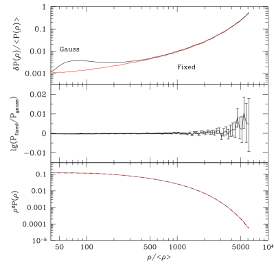
Figure 2: Density distribution function. Bottom panel: $P(\rho)$ scaled with $\rho^{2}$ to reduce the dynamical range. Middle panel: The ratio of the average PDF of paired-and-fixed simulations to those of true Gaussian simulations. Top panel: The r.m.s. scatter of the PDF of individual realisations relative to the ensemble average PDF. There are no detectable differences in the average PDFs even at very high densities with $\rho/\langle\rho\rangle\approx 6000$, where there are only 2-3 such cells in each realisation. The paired-and-fixed simulations decrease the noise of the PDF by a factor of $\sim 1.5$ at large densities near $\rho/\langle\rho\rangle\sim 70$, but this merely suppresses a scatter that was very small to begin with. The noise is orders of magnitude larger at the high-density end of the PDF, where there is no reduction in the noise by using paired-and-fixed simulations.

5 Covariance matrix of the power spectrum

The covariance matrix $C(k,k^{\prime})$ is the second-order statistic of the power spectrum. The power spectrum covariance and its cousin, the covariance of the correlation function, play a key role in estimating the accuracy of the power spectrum measured from large galaxy surveys. Furthermore, the inverse covariance matrices are used to estimate the cosmological parameters inferred from these measurements (e.g., Anderson et al., 2012; Sánchez et al., 2012; Dodelson & Schneider, 2013; Percival et al., 2014). The power spectrum covariance matrix measures the degree of non-linearity and mode coupling of waves with different wavenumbers. As such it is an interesting entity on its own.

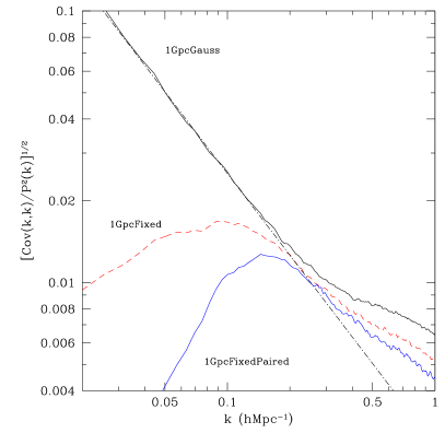
Figure 3: Diagonal components of the covariance matrix $C(k,k)$ of the dark matter power spectrum at redshift $z=0$. Results are normalised to the signal $P^{2}(k)$ as indicated in the plot. For true Gaussian simulations (1GpcGauss, top full curve) the covariance matrix at $k\mbox{${\,\hbox{\hbox{$<$}\kern-8.00003pt\lower 4.30554pt\hbox{$\sim$}}\,}$}0.1\,h{\rm Mpc}^{-1}$ is dominated by the shot-noise due to the finite number of harmonics in a given bin (dot-dashed curve). At larger wavenumbers the covariance matrix is dominated by non-linear effects. At small wavenumbers $k\mbox{${\,\hbox{\hbox{$<$}\kern-8.00003pt\lower 4.30554pt\hbox{$\sim$}}\,}$}0.1\,h{\rm Mpc}^{-1}$ the fixed (1GpcFixed, dashed line) and paired-and-fixed (1GpcPairedFixed, bottom full curve) simulations produce much smaller r.m.s. fluctuations of $P(k)$ per individual realisation. The r.m.s of 1GpcFixed is 20 times smaller at $k=0.02\,h{\rm Mpc}^{-1}$, implying that one would need 400 times more true Gaussian simulations to reach the same level of errors in the average power spectrum. However, the difference in the diagonal components of the covariance matrix decreases dramatically with scale. For example, at $k=0.5\,h{\rm Mpc}^{-1}$ the r.m.s. fluctuation of the 1GpcFixedPaired power spectrum is just 20 per cent lower as compared to the Gaussian simulations.

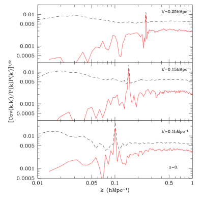
Figure 4: Covariance matrix $C(k,k\prime)$ normalised to the signal $P(k)P(k^{\prime})$ as indicated in the plot. The plot shows three cuts of the non-diagonal components at redshift $z=0$ (from bottom to top): $k^{\prime}=0.10,0.15,0.25\,h{\rm Mpc}^{-1}$. Full curves show the results for the 1GpcPairedFixed simulations. 1GpcGauss simulations are represented by dashed curves. As we showed in Figure 3 for the diagonal components, the non-diagonal terms here show a substantial suppression at small scales and smaller differences at larger wavelengths. The differences are scale-dependent, indicating that it would be difficult to build a mock galaxy catalog from paired-and-fixed simulations that would faithfully recover the true Gaussian covariance matrix.

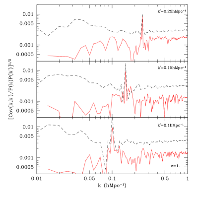
Figure 5: The same as in Figure 4, but at redshift $z=1$. Because the amplitude of fluctuations is smaller at higher redshifts, the covariances at $z=1$ are significantly noisier compared with $z=0$.

The covariance matrix $C(k,k^{\prime})$ is defined as a reduced cross product of power spectra at different wavenumbers in the same realisation averaged over different realisations, i.e.

$$C(k,k^{\prime})\equiv\langle P(k)P(k^{\prime})\rangle-\langle P(k)\rangle\langle P(k^{\prime})\rangle.$$ (7)

The diagonal and non-diagonal components of the covariance matrix typically have very different magnitudes and evolve differently with redshift. The diagonal elements are larger than the off-diagonal ones, but there are many more off-diagonal elements, making them cumulatively important (Taylor et al., 2013; Percival et al., 2014; O’Connell et al., 2016). Off-diagonal elements are solely due to non-linear clustering effects: in a statistical sense the off-diagonal elements are equal to zero in the linear regime. The diagonal component $C(k,k)$ can be written as a sum of Gaussian fluctuations, due to the finite number of harmonics in a given bin, and a term that is due to the non-linear growth of fluctuations, i.e.,

$$C(k,k)\equiv C_{\rm Gauss}(k)+C_{\rm non}(k,k),$$ (8)

where the Gaussian term depends on the amplitude of the power spectrum $P(k)$ and on the number of harmonics $N_{h}$ as

$$C_{\rm Gauss}(k)=\frac{2}{N_{h}}P^{2}(k),\quad N_{h}=\frac{4\pi k^{2}\Delta k}{\left(2\pi/L\right)^{3}}.$$ (9)

Note that for a fixed bin width $\Delta k$ the number of harmonics is proportional to the computational volume, $N_{h}\propto L^{3}$, and thus the amplitude of the Gaussian term scales as $C_{\rm Gauss}(k)\propto 1/L^{3}$ (see Klypin & Prada, 2018).

Figure 3 presents the diagonal components of the covariance matrix. As expected, the true Gaussian simulations closely follow $C_{\rm Gauss}(k)$ at small wavenumbers $k\mbox{${\,\hbox{\hbox{$<$}\kern-8.00003pt\lower 4.30554pt\hbox{$\sim$}}\,}$}0.1\mbox{$\,h$Mpc${}^{-1}$}$, while the paired-and-fixed simulations show a dramatic reduction in the scatter of the power spectrum $P(k)$. However, the situation changes in the non-linear regime $k\mbox{${\,\hbox{\hbox{$>$}\kern-8.00003pt\lower 4.30554pt\hbox{$\sim$}}\,}$}0.2\mbox{$\,h$Mpc${}^{-1}$}$. There, the covariance matrix $C(k,k)$ of the paired-and-fixed simulations increases substantially and becomes only $\sim 20$ per cent smaller than the Gaussian simulations. In addition, the ratio of the covariance matrices is $k$-dependent.

The non-diagonal components $C(k,k^{\prime})$ of the covariance matrix show a similarly complicated trend as demonstrated by Figure 4 and Figure 5 for $z=0$ and $z=1$, respectively: the ratio of the covariances is scale-dependent with large differences at small scales that become smaller for wavenumbers $k\mbox{${\,\hbox{\hbox{$>$}\kern-8.00003pt\lower 4.30554pt\hbox{$\sim$}}\,}$}0.1\mbox{$\,h$Mpc${}^{-1}$}$. One might imagine that the difference between the covariances can be modeled such that the true covariance can be recovered through a rescaling of the covariance from paired-and-fixed simulations. However, this does not seem to be a feasible path forward, not only because of the complicated scale- and redshift-dependence of the differences, but also because the paired-and-fixed $C(k,k^{\prime})$ is much noisier than the Gaussian simulations. In order to reach the same level of noise one would need to make many more realisations of paired-and-fixed simulations, which seems to defeat the motivation for the paired-and-fixed simulations in the first place, i.e., to reduce dramatically the need for many realisations.

6 Bispectrum

The bispectrum is defined as a product of amplitudes of Fourier harmonics at three wavenumbers: $B(k_{1},k_{2},k_{3})=\langle\delta_{k_{1}}\delta_{k_{2}}\delta_{k_{3}}\rangle$. It is convenient to scale out the main dependence on the power spectrum, and define the reduced bispectrum as

$$B_{reduced} =\frac{\langle\delta_{k_{1}}\delta_{k_{2}}\delta_{k_{3}}\rangle}{P(k_{1})P(k_{2})+P(k_{2})P(k_{3})+P(k_{1})P(k_{3})},$$ (10)

where the $P(k_{i})$ in the denominator are the average power spectra.

Four slices of the average reduced bispectrum at $z=0$ are presented in Figure 6 for the set of $3\,\mbox{$h^{-1}$Gpc}$ simulations (see Table 1). Each slice assumes a fixed combination of $k_{1}$ and $k_{2}$ while $k_{3}$ is allowed to vary. The two panels on the left show the average bispectrum for small wavenumbers, while the right panels focus on shorter wavelengths around the BAO scale. Just as we observed for the average power spectrum, we do not find any differences between Gaussian and paired-and-fixed simulations in the wavenumber domain discussed here.

Figure 7 shows the scatter of the bispectrum represented by the diagonal components of the covariance matrix. The results follow the same trend as for the diagonal components of the power spectrum covariance matrix. The scatter is significantly suppressed for very long wavelengths with $k_{1}=0.02\mbox{$\,h$Mpc${}^{-1}$}$ and $k_{2}=0.04\mbox{$\,h$Mpc${}^{-1}$}$ (upper left panel), and it decreases at shorter wavelengths (bottom left panel). At larger wavenumbers (right panels), the differences disappear. We note that this particular feature is unlike the power spectrum covariance, for which the paired-and-fixed simulations always had a scatter that was suppressed relative to the Gaussian simulations.

Figure 6: Average reduced bispectrum of dark matter at $z=0$ for four slices with values of fixed $k_{1}$ and $k_{2}$ as indicated in the panels. Full curves show the results of 1300 realisations of Gaussian simulations (3GpcGauss). Points with error bars are the results from the combined 3GpcFixed and 3GpcPairedFixed simulations (a total of 50 realisations). There are no statistically significant differences between true Gaussian and paired-and-fixed simulations.

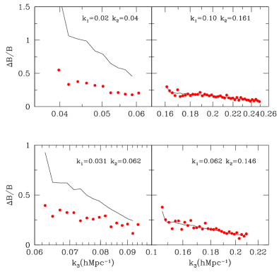
Figure 7: The r.m.s. fluctuations of the reduced bispectrum for a single realisation relative to the average bispectrum for the same slices as in Figure 6. At very long wavelengths the noise in the bispectrum is a factor of three lower for the paired-and-fixed simulation (top-left panel). The difference becomes smaller for even slightly shorter wavelengths (bottom-left panel) and disappear entirely in the domain of BAOs, $k=(0.07-0.30)\,h{\rm Mpc}^{-1}$ (top-right and bottom-right panels).

7 Conclusions

Making accurate theoretical predictions for the clustering statistics of large-scale galaxy surveys is a very relevant but challenging process (e.g., Mandelbaum et al., 2013; Rodríguez-Torres et al., 2016; MacCrann et al., 2018; van Uitert et al., 2018). One of the main goals is to estimate the scatter and covariance errors of measured clustering properties such as the power spectrum and bispectrum: one needs to know the covariances in order to estimate the uncertainties of the inferred cosmological parameters. However, computing the covariance matrices with sufficient accuracy typically requires thousands of realisations, which makes the process quite computationally expensive.

There are tools to create realisations quickly. These include a new generation of faster $N$-body codes (Tassev et al., 2015; Koda et al., 2016; Klypin & Prada, 2018) and approximate methods (Kitaura et al., 2016; Monaco, 2016; Baumgarten & Chuang, 2018; Lippich et al., 2019). An alternative approach proposed by Angulo & Pontzen (2016) has recently attracted attention: the amplitudes of the Fourier harmonics are fixed to be exactly equal to the average amplitude expected for a given cosmological model with true Gaussian fluctuations. Thus, in the linear regime, even a single realisation with fixed harmonics will have exactly the same power spectrum as the average power spectrum obtained from many realisations of true Gaussian-distributed harmonics. A further reduction in the scatter is achieved by running fixed simulations in pairs, where the simulations in a pair have harmonics with opposite phases.

The density field generated by the fixed amplitude method is still a random field: the amplitudes of the Fourier harmonics are random numbers with values equal to either one or minus one (see eq. (3)). As a result, there will be some randomness of fluctuations, but it is strongly suppressed and develops mainly due to non-linear interactions (Villaescusa-Navarro et al., 2018). Thus, paired-and-fixed simulations seem to be a promising direction to reduce scatter due to cosmic variance and, crucially, to reduce the number of realisations for estimates of different statistics. However, there are still remaining questions and concerns about the effect of fixing the amplitudes of the harmonics. What happens in the non-linear regime? If the realisation-to-realisation scatter is suppressed, at least in the linear regime, and the scatter is only the diagonal component of the covariance matrices, how are the full covariances affected by fixing the amplitudes of the Fourier harmonics?

There is a clear answer to one of these questions. Every average clustering statistic studied in this paper, and in other works, is not affected in any measurable way by paired-and-fixed simulations as compared to those obtained from true Gaussian perturbations. The list of statistics is long and includes: the power spectrum, halo mass function, correlation function, density distribution function and bispectrum (this paper, Angulo & Pontzen, 2016; Villaescusa-Navarro et al., 2018; Chuang et al., 2018). It is very promising for the paired-and-fixed method that there are no defects, at least for the average statistics.

This is despite the fact that paired-and-fixed fluctuations are clearly not what one expects for initial conditions in the real Universe. The real fluctuations generated during inflation should not have fixed amplitudes, so why do paired-and-fixed simulations give the correct answers for so many different average statistics? The apparent success of the method is related to the fact that the statistics of interest are typically large sums of many contributions from different Fourier harmonics. Then, by the virtue of the central limit theorem, the distribution function of these statistics is as Gaussian as that from truly Gaussian fields in inflationary models. As an example, we can consider the density field $\delta({\mn@boldsymbol{x}})$. It is a sum of many harmonics, as shown in eqs. (1–4). Thus, the distribution function of $\delta({\mn@boldsymbol{x}})$ and its two-point correlation function $\langle\delta({\mn@boldsymbol{x}})\delta({\mn@boldsymbol{x}}+{\mn@boldsymbol{r}})\rangle$ are the same as for a true Gaussian density field. Because the initial density field, together with the adopted cosmological parameters, define how the different structures evolve and collapse in the expanding Universe, it is not surprising that many average properties (e.g., correlations functions or halo mass functions) are correctly recovered.

How much of a reduction in the realisation-to-realisation scatter that one gains by performing paired-and-fixed simulations depends on the degree of non-linear growth, and consequently on the physical scale. For example, at $k=0.05\mbox{$\,h$Mpc${}^{-1}$}$ the r.m.s. fluctuation of the power spectrum is ten times smaller in paired-and-fixed simulations (see Figure 3). Because the error of the average power spectra in Gaussian simulations declines as $1/\sqrt{N_{r}}$, where $N_{r}$ is the number of realisations, one would need 100 times more Gaussian realisations to reach the same accuracy as the average power spectrum from paired-and-fixed simulations. A large reduction of noise is similarly observed for the bispectrum: the r.m.s. fluctuations are reduced by a factor of three for $(k_{1},k_{2},k_{3})=(0.02,0.04,0.04)\mbox{$\,h$Mpc${}^{-1}$}$ (see Figure 7).

Unfortunately, these gains in the number of realisations diminish dramatically with scale. In the BAO spectral domain $k=0.07-0.3\,h{\rm Mpc}^{-1}$, the r.m.s. fluctuations of the power spectrum are smaller in the paired-and-fixed simulations by only $\sim 20$ per cent compared to the purely Gaussian realisations. The r.m.s. scatter in the bispectrum shows an even smaller effect: it is the same as in Gaussian simulations for $k\mbox{${\,\hbox{\hbox{$>$}\kern-8.00003pt\lower 4.30554pt\hbox{$\sim$}}\,}$}0.1\mbox{$\,h$Mpc${}^{-1}$}$ (right panels in Figure 7). Similar results are found for those statistics that are more sensitive to strongly non-linear interactions. Paired-and-fixed simulations offer no advantage for the halo mass function (Villaescusa-Navarro et al., 2018), and we do not see any gains for the density distribution function (see Figure 2).

One of the main goals and challenges for any simulation method is to accurately capture the scatter and covariances of clustering statistics, but in this work we find that this poses a difficult issue for paired-and-fixed simulations. As Figure 3 shows, even the scatter of the power spectrum (the diagonal component of the covariance matrix) presents a problem, because the difference in the scatter with respect to true Gaussian simulations depends on the wavenumber $k$ in a complicated way. One might consider fitting these differences with an analytical approximation in order to recover the true scatter. However, this would not work because that difference depends on redshift and must be done for the distribution of mock galaxies, that in turn requires numerous realisations to be estimated accurately enough.

The non-diagonal components of the power spectrum covariance matrix (Figures 4 and 5) point to another complication for the paired-and-fixed simulations. Just as for the scatter of the power spectrum, the ratio of non-diagonal components of paired-and-fixed to Gaussian simulations depends on scale and redshift in a non-trivial way. In addition, the covariance matrix of paired-and-fixed simulations is much noisier than for purely Gaussian simulations with the same number of realisations. In order to reach the same level of noise one would need to make many more paired-and-fixed realisations, which defeats the main motivation behind this method.

The main results of our work are summarised as follows:

• Paired-and-fixed simulations accurately reproduce the average of the power spectrum, PDF and bispectrum from Gaussian simulations.

• The reduction in cosmic variance error obtained from paired-and-fixed simulations is limited to very long-wavelengths with $k\mbox{${\,\hbox{\hbox{$<$}\kern-8.00003pt\lower 4.30554pt\hbox{$\sim$}}\,}$}0.05\mbox{$\,h$Mpc${}^{-1}$}$. Non-linear effects erase most of the advantage from pairing and fixing, even in the weakly non-linear domain $k\mbox{${\,\hbox{\hbox{$>$}\kern-8.00003pt\lower 4.30554pt\hbox{$\sim$}}\,}$}0.1\mbox{$\,h$Mpc${}^{-1}$}$.

• Paired-and-fixed simulations fail to provide a path towards reproducing the true Gaussian covariance errors. Not only are the reported differences with Gaussian simulations scale- and redshift-dependent, but covariances from paired-and-fixed simulations are also much noisier and would require many more realisations to reach the same level of accuracy as obtained from Gaussian simulations.

Because accurate covariance errors are crucial for robustly translating the observed clustering statistics from large galaxy surveys into constraints on cosmological parameters, the results presented in this paper demonstrate that paired-and-fixed simulations are not suitable for generating mock galaxy catalogs, but they are a very useful tool for quickly and accurately estimating the average properties of the clustering signal.

References

- Anderson et al. (2012) Anderson L. et al., 2012, MNRAS, 427, 3435
- Angulo & Pontzen (2016) Angulo R. E., Pontzen A., 2016, MNRAS, 462, L1
- Bartolo et al. (2004) Bartolo N., Komatsu E., Matarrese S., Riotto A., 2004, Phys.Rep., 402, 103
- Baumgarten & Chuang (2018) Baumgarten F., Chuang C.-H., 2018, MNRAS, 480, 2535
- Binney & Tremaine (2008) Binney J., Tremaine S., 2008, Galactic Dynamics: Second Edition. Princeton University Press
- Chuang et al. (2018) Chuang C.-H. et al., 2018, arXiv e-prints
- Conroy et al. (2006) Conroy C., Wechsler R. H., Kravtsov A. V., 2006, ApJ, 647, 201
- Dodelson & Schneider (2013) Dodelson S., Schneider M. D., 2013, Phys. Rev. D, 88, 063537
- Feng et al. (2016) Feng Y., Chu M.-Y., Seljak U., 2016, ArXiv e-prints
- Izard et al. (2015) Izard A., Crocce M., Fosalba P., 2015, ArXiv e-prints
- Kitaura et al. (2016) Kitaura F.-S. et al., 2016, MNRAS, 456, 4156
- Klypin & Prada (2018) Klypin A., Prada F., 2018, MNRAS, 478, 4602
- Koda et al. (2016) Koda J., Blake C., Beutler F., Kazin E., Marin F., 2016, MNRAS, 459, 2118
- Lippich et al. (2019) Lippich M. et al., 2019, MNRAS, 482, 1786
- MacCrann et al. (2018) MacCrann N. et al., 2018, MNRAS, 480, 4614
- Mandelbaum et al. (2013) Mandelbaum R., Slosar A., Baldauf T., Seljak U., Hirata C. M., Nakajima R., Reyes R., Smith R. E., 2013, MNRAS, 432, 1544
- Monaco (2016) Monaco P., 2016, Galaxies, 4, 53
- Mukhanov et al. (1992) Mukhanov V. F., Feldman H. A., Brandenberger R. H., 1992, Phys.Rep., 215, 203
- O’Connell et al. (2016) O’Connell R., Eisenstein D., Vargas M., Ho S., Padmanabhan N., 2016, MNRAS, 462, 2681
- Percival et al. (2014) Percival W. J. et al., 2014, MNRAS, 439, 2531
- Pontzen et al. (2016) Pontzen A., Slosar A., Roth N., Peiris H. V., 2016, Phys. Rev. D, 93, 103519
- Rodríguez-Torres et al. (2016) Rodríguez-Torres S. A. et al., 2016, MNRAS, 460, 1173
- Sánchez et al. (2012) Sánchez A. G. et al., 2012, MNRAS, 425, 415
- Somerville & Davé (2015) Somerville R. S., Davé R., 2015, Ann.Rev.Astrn.Astrophys., 53, 51
- Somerville & Primack (1999) Somerville R. S., Primack J. R., 1999, MNRAS, 310, 1087
- Tassev et al. (2015) Tassev S., Eisenstein D. J., Wandelt B. D., Zaldarriaga M., 2015, ArXiv e-prints
- Taylor et al. (2013) Taylor A., Joachimi B., Kitching T., 2013, MNRAS, 432, 1928
- Trujillo-Gomez et al. (2011) Trujillo-Gomez S., Klypin A., Primack J., Romanowsky A. J., 2011, ApJ, 742, 16
- van Uitert et al. (2018) van Uitert E. et al., 2018, MNRAS, 476, 4662