Spin dynamics of antiferromagnetically coupled ferromagnetic bilayers – the case of Cr₂WO₆ and Cr₂MoO₆

Abstract

Recent inelastic neutron diffraction measurements on Cr₂(Te, W, Mo)O₆ have revealed that these systems consist of bilayers of spin-3/2 Cr³⁺ ions with strong antiferromagnetic inter-bilayer coupling and tuneable intra-bilayer coupling from ferro (for W and Mo) to antiferro (for Te). These measurements have determined the ground state spin structure and the values of sublattice magnetization, which shows significant reduction of sublattice magnetization from the atomic spin value of 3.0$\mu_{B}$ for Cr³⁺ atoms. In an earlier paper we theoretically investigated the low temperature spin dynamics of Cr₂TeO₆ bilayer system where both the intra and inter-bilayer couplings are antiferromagnetic. In this paper we investigate Cr₂WO₆ and Cr₂MoO₆ systems where intra-bilayer exchange couplings are ferromagnetic but the inter-bilayer exchange couplings are antiferromagnetic. We obtain the magnon dispersion, sublattice magnetization, two-magnon density of states, longitudinal spin-spin correlation function, and its powder average and compare the results for these systems with results for Cr₂TeO₆.

I Introduction and Formalism

Exploring the dynamics of quantum spins with competing interactions and geometrical frustration has been one of the most exciting areas of theoretical and experimental research over last several decades. Anderson (1952); Harris et al. (1971); Diep (2004); Lacroix et al. (2011); Rastelli (2013); Majumdar (2010, 2011a, 2011b); Majumdar et al. (2012); Uhrig and Majumdar (2013) A subset of this research is understanding the physics of interacting quantum spin dimers (QSD), where the intra-dimer interaction is antiferromagnetic (strength $J$). Sachdev (2001); Zhu et al. (2014); Mahanti and Kaplan (1991) By tuning the geometry and the strength of inter-dimer coupling ($j$), the system can go from strongly fluctuating zero-dimensional to quasi $n$ ($n=1,2,3$) dimensional system, accompanied by dramatic changes in spin dynamics. Zhu et al. (2014, 2015)

Some of the interesting observations for the ground state of interacting quantum spins (IQS) are: absence of long range order (LRO) and long range quantum spin entanglement i.e. a liquid like structure (for example, Haldane state for 1D chains with integer spins, Luttinger Fermi-liquid for half-integer spins) in 1D even at $T=0$K or dramatic reduction in the LRO moment in 2D due to quantum fluctuations. The excitations also span a broad range, from spinons to triplons to magnons. These theoretical developments have lead to the synthesis of many interesting insulating magnetic systems where the spin dimensionality, space dimensionality, inter-spin coupling can be tuned. Experimental studies in these systems have deepened our fundamental understanding of the physics of IQS systems. Diep (2004); Lacroix et al. (2011); Rastelli (2013); Sachdev (2001); Ronnow et al. (2001); Christensen et al. (2004, 2007)

In a particular class of IQS, one of present interest, the system consists of quantum spin dimers (QSDs). Depending on the nature of the super exchange coupling between the localized magnetic moments, the dominant interaction is the intra-dimer coupling $J$. In this case, the magnetic centers are QSDs with antiferromagnetic $J$ weakly interacting with each other through $j$. If, on the other hand, the interaction between the QSDs is stronger than $J$, then the system can be thought of as 2$D$ ferro- or antiferro-magnetic sheets with antiferromagnetic inter-sheet coupling. In fact, by manipulating local chemistry one can tune this coupling from F to AF, going through effectively non-interacting ($j=0$) QSDs. Zhu et al. (2014, 2015)

The focus of this paper is to explore the effect of changing the sign and strength of $j$ on the ground and excited states using the example of a Cr based system, Cr₂XO₆ (X= Te, W, Mo). On theoretical ground one expects the system to undergo a quantum phase transition from a quantum disordered state to a state with LRO as $|j|$ is increased. The latter state supports magnon excitations. If one is not too far from the critical region then the resulting soft magnons reduce the LRO moment. How the magnon dispersion and reduction in the moment depends on the sign of $j$ are interesting questions that we explore in this paper. It is experimentally found that in Cr₂TeO₆, $j$ is anti-ferromagnetic whereas in Cr₂WO₆ and Cr₂MoO₆, $j$ is ferromagnetic. Zhu et al. (2015) This unusual observation was explained by ab initio density functional theory based calculations of different magnetically ordered states in these compounds, and was ascribed to the presence of low energy unoccupied $d$-states in W and Mo, an idea similar to $d$-zeroness in ferroelectricity. Filippetti and Hill (2002) In spite of the fact that $J$ is the dominant exchange coupling, due to sufficiently large $|j|$ and the number of inter-dimer bonds, these systems show LRO and the excitations are magnon-like. In addition to magnon modes there is strong experimental evidence of Higgs-like amplitude modes, a characteristics of interacting QSDs. Zhu et al. (2015) Here we will discuss only the magnon-like excitations. The case of antiferromagnetic $j$ has been extensively discussed in an earlier paper by us. Majumdar and Mahanti (2018) In this paper, we will discuss the results for the ferromagnetic case briefly focusing on the similarities and differences between the two cases.

In Fig. 1 we show the ground state spin ordering in Cr₂(X=W, Mo)O₆. Kunnmann et al. (1968) One has two bilayers (perpendicular to the $z$-axis) in the tetragonal unit cell $(a,a,c)$ and four Cr spins/unit cell. The experimental unit cell parameters for Cr₂WO₆ are $a=4.583$Å,  $c=8.853$Å  and $a=4.587$Å, $c=8.811$Å  for Cr₂MoO₆ at $T=4$K. Zhu et al. (2014) The Cr-O-Cr bond angles and bond lengths of both of these compounds are similar due to the similar ionic radii of Mo⁶⁺ and W⁶⁺. The shortest distance between the inter-bilayer (NN) Cr atoms i.e. Cr1 and Cr3 is $\delta\sim 3.00$Å $\approx c/3$, whereas the distance between intra-bilayer NN Cr atoms (Cr1 and Cr2 or Cr3 and Cr4) is $\sim 3.80$Å. One bilayer contains Cr1 and Cr2 spins and the other contains Cr3 and Cr4 spins. The inter-bilayer AF coupling $J$ comes through Cr1-Cr3 and Cr2-Cr4 dimers. The NN intra-bilayer ferromagnetic coupling $j$ is between Cr3-Cr4 and Cr1-Cr2. Estimates of exchange parameters from high temperature thermodynamic measurements Drillon et al. (1979) indicate that $|j|,|j^{\prime}|<<|J|$ – so these systems can be regarded as weakly interacting quantum dimers.

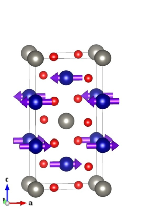
(a)   (b)

Figure 1: (Color online)(a) Schematic of the bilayer crystal structure and magnetic ordering of Cr₂(Mo, W)O₆. Each Cr³⁺ (blue spheres) bilayer is separated by a W/Mo (grey spheres) layer. Zhu et al. (2014, 2015) The oxygen (O) atoms are shown by the red spheres. (b) Positions of four chromium spins in the tetragonal unit cell of dimensions $(a,a,c)$ are shown. The coordinates of the spins are given in Ref.Majumdar and Mahanti, 2018.

In this paper we calculate magnon dispersion, sublattice magnetization, two-magnon density of states, longitudinal spin-spin correlation function, and it’s powder average using linear spin-wave theory. Majumdar (2010); Majumdar et al. (2012) Our current work is for a completely different class of systems with different ground state spin configuration than our recently published work on Cr₂TeO₆. Majumdar and Mahanti (2018) In this paper we briefly provide the theoretical formalism in Appendix A and present only the relevant equations and results pertinent to the current systems.

I.1 Magnon Dispersion and Sublattice Magnetization

The Heisenberg Hamiltonian of systems with F intra- and AF inter-bilayer couplings $j,j^{\prime}$, and $J$ ($j,\;j^{\prime},\;J>0$) has the form

$${\cal H}={\cal H}_{\rm NN}+{\cal H}_{\rm NNN},$$ (1)

with

$${\cal H}_{\rm NN} = -j\sum_{n=1}^{N_{z}}\sum_{\langle i,j\rangle}\Big{[}{\bf S}_{in}^{(1)A}\cdot{\bf S}_{jn}^{(2)A}+{\bf S}_{in}^{(3)B}\cdot{\bf S}_{jn}^{(4)B}\Big{]}$$ (2a)

$$+ J\sum_{n=1}^{N_{z}}\sum_{i}\Big{[}{\bf S}_{in}^{(1)A}\cdot{\bf S}_{in}^{(3)B}+\frac{1}{2}\{{\bf S}_{in}^{(2)A}\cdot{\bf S}_{in-1}^{(4)B}+{\bf S}_{in}^{(4)B}\cdot{\bf S}_{in+1}^{(2)A}\}\Big{]},$$

$${\cal H}_{\rm NNN} = -j^{\prime}\sum_{n=1}^{N_{z}}\sum_{\langle\langle i,j\rangle\rangle}\Big{[}{\bf S}_{in}^{(1)A}\cdot{\bf S}_{jn}^{(1)A}+{\bf S}_{in}^{(2)A}\cdot{\bf S}_{jn}^{(2)A}+{\bf S}_{in}^{(3)B}\cdot{\bf S}_{jn}^{(3)B}+{\bf S}_{in}^{(4)B}\cdot{\bf S}_{jn}^{(4)B}\Big{]}.$$ (2b)

After Holstein-Primakoff transformation Holstein and Primakoff (1940) and Fourier transform, the quadratic part of the Hamiltonian represented in terms of interacting bosons $a$ and $b$ takes the form (the details are shown in Appendix A):

$${\cal H}_{0} = jS(4+\eta)\sum_{\bf k}\kappa_{\bf k}\Big{[}\Big{(}a_{\bf k}^{{(1)}\dagger}a_{\bf k}^{(1)}+a_{\bf k}^{{(2)}\dagger}a_{\bf k}^{(2)}+b_{-\bf k}^{{(3)}\dagger}b_{-\bf k}^{(3)}+b_{-\bf k}^{{(4)}\dagger}b_{-\bf k}^{(4)}\Big{)}$$ (3)

$$- \gamma_{1\bf k}\Big{(}a^{(1)}_{\bf k}a^{(2)\dagger}_{\bf k}+b^{(3)}_{-\bf k}b^{(4)\dagger}_{-\bf k}\Big{)}-\gamma_{1\bf k}^{*}\Big{(}a^{(2)}_{\bf k}a^{(1)\dagger}_{\bf k}+b^{(4)}_{-\bf k}b^{(3)\dagger}_{-\bf k}\Big{)}$$

$$+ \gamma_{2\bf k}\Big{(}a^{(2)}_{\bf k}b^{(4)}_{-\bf k}+a^{(1)\dagger}_{\bf k}b^{(3)\dagger}_{-\bf k}\Big{)}+\gamma_{2\bf k}\Big{(}a^{(1)}_{\bf k}b^{(3)}_{-\bf k}+a^{(2)\dagger}_{\bf k}b^{(4)\dagger}_{-\bf k}\Big{)}\Big{]},$$

where,

$$\gamma_{1\bf k} = \frac{4}{4+\eta}\frac{e^{ik_{z}c/2}\cos(k_{x}a/2)\cos(k_{y}a/2)}{1+\gamma_{3\bf k}},$$

$$\gamma_{2\bf k} = \frac{\eta}{4+\eta}\frac{1}{1+\gamma_{3\bf k}},$$

$$\gamma_{3\bf k} = \frac{4\eta^{\prime}}{4+\eta}[1-\frac{1}{2}(\cos(k_{x}a)+\cos(k_{y}a))],$$

$$\kappa_{\bf k} = 1+\gamma_{3\bf k}.$$ (4)

Above, $\eta=J/j$ and $\eta^{\prime}=j^{\prime}/j$. ${\cal H}_{0}$ in Eq. (3) can be succinctly written as ${\cal H}_{0}={\cal H}_{1}\oplus{\cal H}_{1}^{\rm T}$ where ${\cal H}_{1}^{\rm T}$ is the transpose of ${\cal H}_{1}$. In the Fourier transformed basis $X_{\bf k}=(a_{\bf k}^{(1)}\;a_{\bf k}^{(2)}\;b_{-\bf k}^{(4)\dagger}\;b_{-\bf k}^{(3)\dagger})^{T}$ we write ${\cal H}_{1}$ as

$${\cal H}_{1}=jS(4+\eta)\sum_{\bf k}\kappa_{\bf k}X_{\bf k}^{\dagger}{\cal H}_{1\bf k}^{\prime}X_{\bf k}$$ (5)

with

$${\cal H}_{1\bf k}^{\prime}=\begin{bmatrix}A_{\bf k}&B_{\bf k}&0&C_{\bf k}\\ B_{\bf k}^{\star}&A_{\bf k}&C_{\bf k}&0\\ 0&C_{\bf k}&A_{\bf k}&B_{\bf k}\\ C_{\bf k}&0&B_{\bf k}^{\star}&A_{\bf k}\end{bmatrix}$$ (6)

and $A_{\bf k}=1,B_{\bf k}=-\gamma_{1\bf k}^{\ast},C_{\bf k}=\gamma_{2{\bf k}}$. Next, we diagonalize ${\cal H}_{1}$ by transforming the operators $a_{\bf k}$ and $b_{\bf k}$ to magnon operators $\alpha_{\bf k}$ and $\beta_{\bf k}$ using the following generalized Bogoliubov (BG) transformations Bogoliubov (1958); Colpa (1978); Wheeler et al. (2009); Huang et al. (2017):

$$\begin{pmatrix}a_{\bf k}^{(1)}\\ a_{\bf k}^{(2)}\\ b_{-\bf k}^{(4)\dagger}\\ b_{-\bf k}^{(3)\dagger}\end{pmatrix}=\begin{bmatrix}\ell_{1\bf k}&\ell_{1\bf k}^{\prime}&m_{1\bf k}&m_{1\bf k}^{\prime}\\ \ell_{2\bf k}^{\prime}&\ell_{2\bf k}&m_{2\bf k}^{\prime}&m_{2\bf k}\\ m_{1\bf k}&m_{1\bf k}^{\prime}&\ell_{1\bf k}&\ell_{1\bf k}^{\prime}\\ m_{2\bf k}^{\prime}&m_{2\bf k}&\ell_{2\bf k}^{\prime}&\ell_{2\bf k}\end{bmatrix}\begin{pmatrix}\alpha_{\bf k}^{(1)}\\ \alpha_{\bf k}^{(2)}\\ \beta_{-\bf k}^{(1)\dagger}\\ \beta_{-\bf k}^{(2)\dagger}\end{pmatrix}.$$ (7)

The elements of the transformation matrix $\ell_{(1,2)\bf k},\ell_{(1,2)\bf k}^{\prime},m_{(1,2)\bf k},m_{(1,2)\bf k}^{\prime}$ are given in Appendix B.

The quadratic Hamiltonian after diagonalization becomes:

$${\cal H}_{1} = jS(4+\eta)\sum_{\bf k}\kappa_{\bf k}\Big{\{}\omega_{\bf k}^{(1)}\Big{[}\alpha_{\bf k}^{(1)\dagger}\alpha_{\bf k}^{(1)}+\beta_{-\bf k}^{(1)\dagger}\beta_{-\bf k}^{(1)}\Big{]}+\omega_{\bf k}^{(2)}\Big{[}\alpha_{\bf k}^{(2)\dagger}\alpha_{\bf k}^{(2)}+\beta_{-\bf k}^{(2)\dagger}\beta_{-\bf k}^{(2)}\Big{]}\Big{\}}$$ (8)

$$- jS(4+\eta)\sum_{\bf k}\kappa_{\bf k}\Big{[}\omega^{(1)}_{\bf k}+\omega^{(2)}_{\bf k}-2\Big{]}.$$

${\cal H}_{1}^{T}$ has the same structure as ${\cal H}_{1}$. The two roots in Eq. (8) are: Wheeler et al. (2009); Huang et al. (2017)

$$\omega_{\bf k}^{(1,2)}=\Big{[}A_{\bf k}^{2}+|B_{\bf k}|^{2}-C_{\bf k}^{2}\mp\sqrt{4A_{\bf k}^{2}|B_{\bf k}|^{2}-C_{\bf k}^{2}|B_{\bf k}^{\star}-B_{\bf k}|^{2}}\;\Big{]}^{1/2}.$$ (9)

For our case, the eigenvalues for the $\alpha$ and $\beta$ magnon branches (a low energy acoustic branch and a high energy optic branch) simplify to

$$\omega_{\bf k}^{(1,2)}=\Big{[}1+|\gamma_{1\bf k}|^{2}-\gamma_{2\bf k}^{2}\mp\sqrt{4|\gamma_{1\bf k}|^{2}-\gamma_{2\bf k}^{2}|\gamma_{1\bf k}-\gamma_{1\bf k}^{*}|^{2}}\;\Big{]}^{1/2}$$ (10)

and the quasiparticle energies $E_{\bf k}^{(1,2)}$ for these magnons are given by:

$$E_{\bf k}^{(1,2)}=jS(4+\eta)\kappa_{\bf k}\omega_{\bf k}^{(1,2)}.$$ (11)

The second term in Eq. (8) is the quantum-zero point energy, which contributes to the ground state energy. In order to understand the physical origin of the two modes with frequencies $\omega_{\bf k}^{(1)}$ and $\omega_{\bf k}^{(2)}$, each two-fold degenerate (for the full quadratic ${\cal H}_{0}$), we start from the limit when the inter-bilayer coupling $J=0$ and then introduce nonzero $J$. When $J=0$, we have two decoupled ferromagnetic bilayers. In anticipation of antiferromagnetic $J$, we denote one bilayer spins “up” ($\alpha$-magnons) and the other bilayer spins “down” ($\beta$-magnons). They are of course degenerate, each with two modes of frequencies $\omega_{\bf k}^{(1)}$ and $\omega_{\bf k}^{(2)}$. These two modes arise as the unit cell contains two spins of each orientation. For the ferromagnetic ordering we could have chosen a smaller unit cell with one spin/unit cell and one would have obtained one ferromagnetic magnon branch. When mapped on to the smaller BZ associated with larger unit cell (two spins/unit cell) we get two branches. For simplicity, we can refer to these two branches as acoustic and optic branches in analogy with phonons. Thus in the limit $J=0$, we have a two-fold degenerate acoustic branch (one $\alpha$ and one $\beta$) and a two-fold degenerate optic branch (one $\alpha$ and one $\beta$). When we turn on $J$, the degenerate $\alpha$ and $\beta$ branches mix and give rise to new $\alpha$ and $\beta$ branches which preserve their double degeneracy because of time-reversal symmetry, similar to the case of magnons in a simple antiferromagnet.

The normalized sublattice magnetization $m_{s}=M_{s}/M_{0}$ (where $M_{0}=g\mu_{B}$) for the A-sublattice can be expressed as

$$m_{s}=S-\delta S,$$ (12)

where,

$$\delta S=\frac{1}{N}\sum_{\bf k}\langle a^{(1)\dagger}_{\bf k}a^{(1)}_{\bf k}\rangle=\frac{1}{N}\sum_{\bf k}\Big{[}|m_{1\bf k}|^{2}+|m_{1\bf k}^{\prime}|^{2}\Big{]}.$$ (13)

$\delta S$ corresponds to the reduction of magnetization within linear spin-wave theory (LSWT) and the summation over ${\bf k}$ goes over the entire Brillouin zone corresponding to the tetragonal unit cell $(a,a,c)$. The Bogoliubov coefficients $m_{1\bf k}$ and $m_{1\bf k}^{\prime}$ in Eq. (13) are given in Appendix B.

I.2 Two-magnon density of states (TM-DOS) and Longitudinal spin-spin correlation function (LSSCF)

TM-DOS associated with the four magnon branches ($i,j=1,2$) are given as:

$${\rm DOS}_{ij}({\bf k},\omega)=\sum_{\bf{p}}\delta(\omega-\omega^{(i)}_{\bf p}-\omega^{(j)}_{\bf k+p}).$$ (14)

DOS₁₁, DOS₂₂ are the intra-branch and DOS₁₂, DOS₂₁ are the inter-branch density of states. Longitudinal spin-spin correlation function ${\cal L}_{s}({\bf k},\omega)$ is the sum of the weighted $\delta$-functions arising from these four density of states. LSSCF is defined as

$${\cal L}_{s}({\bf k},t)=\langle S_{z}({\bf k},t)S_{z}(-{\bf k},0)\rangle,$$ (15)

with

$$S_{z}({\bf k})=\frac{1}{\sqrt{4N}}\sum_{i\mu}S_{z}^{i\mu}e^{-i{\bf k}\cdot({{\bf R}_{i}}+\tau_{\mu})}.$$ (16)

Here ${\bf R}_{i}$ is the position vector of the $i$-th unit cell and ${\bf\tau}_{\mu}$ are the positions of the four Cr-atoms in the unit cell. The position of the Cr-atoms are respectively: Cr1: $\tau_{1}=(0,0,c/2-\delta/2)$, Cr2: $\tau_{2}=(a/2,a/2,\delta/2)$, Cr3: $\tau_{3}=(0,0,c/2+\delta/2)$, and Cr4: $\tau_{2}=(a/2,a/2,c-\delta/2)$ [See Fig. 1]. Experimentally measured quantity is the Fourier transform of the time-dependent spin-correlation function ${\cal L}_{s}({\bf k},t)$

$${\cal L}_{s}({\bf k},\omega)=\int_{-\infty}^{\infty}\frac{dt}{2\pi}{\cal L}_{s}({\bf k},t)e^{-i\omega t}.$$ (17)

where spins for each of the sublattices $1,2,3,4$ after Fourier transform become:

$$S_{z}^{(\mu=1,2)}({\bf k}) = \sqrt{4N}S\delta({\bf k}=0)-\frac{1}{\sqrt{4N}}\sum_{{\bf p,q}}\delta({\bf k}+{\bf p}-{\bf q})f_{\mu\bf k}a_{\bf p}^{(\mu)\dagger}a_{\bf q}^{(\mu)},$$ (18a)

$$S_{z}^{(\mu=3,4)}({\bf k}) = -\sqrt{4N}S\delta({\bf k}=0)+\frac{1}{\sqrt{4N}}\sum_{{\bf p,q}}\delta({\bf k}+{\bf p}-{\bf q})f_{\mu\bf k}b_{-{\bf q}}^{(\mu)\dagger}b_{-\bf p}^{(\mu)}.$$ (18b)

$f_{\mu{\bf k}}=e^{-i{\bf k\cdot\tau_{\mu}}}$ takes into account the relative phases of the different magntic atoms inside the unit cell. The total spin can now be written as:

$$S_{z}({\bf k})=-\frac{1}{\sqrt{4N}}\sum_{{\bf p,q}}\delta({\bf k}+{\bf p}-{\bf q})\Big{\{}[f_{1\bf k}a_{\bf p}^{(1)\dagger}a_{\bf q}^{(1)}+f_{2\bf k}a_{\bf p}^{(2)\dagger}a_{\bf q}^{(2)}]-[f_{3\bf k}b_{-{\bf q}}^{(3)\dagger}b_{-\bf p}^{(3)}+f_{4\bf k}b_{-{\bf q}}^{(4)\dagger}b_{-\bf p}^{(4)}]\Big{\}}.$$ (19)

Using BG transformations we express $S_{z}({\bf k})$ in terms of the magnon operators $\alpha$ and $\beta$. The result is shown in the Appendix C. There are $16\times 16$ time-ordered Green’s functions that arise from Eq. (15), of which only four shown in Fig. 2 contribute to LSSCF. These are defined in Ref. Majumdar and Mahanti, 2018.

Figure 2: Green’s function propagators for $\alpha$ and $\beta$ magnons (1 and 2) are shown by solid and dashed lines respectively. The Feynman diagram for the four time-ordered Green’s functions $\Pi_{i=1\cdots 4}(\omega)$ that contribute to the longitudinal spin-spin correlation function are shown.

The correlation function ${\cal L}_{s}({\bf k},\omega)$ takes the following form:

$${\cal L}_{s}({\bf k},\omega) = \frac{1}{4N}\Big{[}\sum_{\bf p}\delta(\omega-\omega^{(1)}_{\bf p}-\omega^{(1)}_{\bf p+k})|{\cal D}^{11}_{\bf k,k+p}|^{2}+\sum_{\bf p}\delta(\omega-\omega^{(2)}_{\bf p}-\omega^{(2)}_{\bf p+k})|{\cal D}^{22}_{\bf k,k+p}|^{2}$$ (20)

$$+ \sum_{\bf p}\delta(\omega-\omega^{(2)}_{\bf p}-\omega^{(1)}_{\bf p+k})|{\cal D}^{21}_{\bf k,k+p}|^{2}+\sum_{\bf p}\delta(\omega-\omega^{(1)}_{\bf p}-\omega^{(2)}_{\bf p+k})|{\cal D}^{12}_{\bf k,k+p}|^{2}\Big{]},$$

where the weights $D^{ij}_{{\bf k,k+p}}$ are defined as,

$${\cal D}^{11}_{\bf k,k+p} = [f_{1\bf k}\ell_{1\bf p}^{\ast}m_{1{\bf p+k}}+f_{2\bf k}\ell_{2\bf p}^{\prime\ast}m_{2{\bf p+k}}^{\prime}]-[f_{3\bf k}\ell_{2{\bf p+k}}^{\prime}m_{2\bf p}^{\prime\ast}+f_{4\bf k}\ell_{1{\bf p+k}}m_{1{\bf p}}^{\ast}],$$ (21a)

$${\cal D}^{22}_{\bf k,k+p} = [f_{1\bf k}\ell_{1\bf p}^{\prime\ast}m_{1{\bf p+k}}^{\prime}+f_{2\bf k}\ell_{2\bf p}^{\ast}m_{2{\bf p+k}}]-[f_{3\bf k}\ell_{2{\bf p+k}}m_{2\bf p}^{\ast}+f_{4\bf k}\ell_{1{\bf p+k}}^{\prime}m_{1{\bf p}}^{\ast}],$$ (21b)

$${\cal D}^{21}_{\bf k,k+p} = [f_{1\bf k}\ell_{1\bf p}^{\ast}m_{1{\bf p+k}}^{\prime}+f_{2\bf k}\ell_{2\bf p}^{\prime\ast}m_{2{\bf p+k}}]-[f_{3\bf k}\ell_{2{\bf p+k}}m_{2\bf p}^{\prime\ast}+f_{4\bf k}\ell_{1{\bf p+k}}^{\prime}m_{1{\bf p}}^{\ast}],$$ (21c)

$${\cal D}^{12}_{\bf k,k+p} = [f_{1\bf k}\ell_{1\bf p}^{\prime\ast}m_{1{\bf p+k}}+f_{2\bf k}\ell_{2\bf p}^{\ast}m_{2{\bf p+k}}^{\prime}]-[f_{3\bf k}\ell_{2{\bf p+k}}^{\prime}m_{2\bf p}^{\ast}+f_{4\bf k}\ell_{1{\bf p+k}}m_{1{\bf p}}^{\prime\ast}].$$ (21d)

Smooth TM-DOS and ${\cal L}_{s}({\bf k},\omega)$ are obtained by replacing the $\delta$-function by a Gaussian with a constant broadening width $\sigma$:

$$\sum_{\bf{p}}\delta(\omega-\omega_{\bf p})\rightarrow\sum_{\bf{p}}\frac{1}{\sqrt{2\pi\sigma^{2}}}e^{-(\omega-\omega_{\bf p})^{2}/2\sigma^{2}}.$$ (22)

This Gaussian function accounts for three purposes: (1) finite experimental resolution, (2) experimental uncertainty in the determination of the continua, and (3) finite life time of the measured excitations induced by finite temperature and/or by disorder in the sample. Powalski et al. (2018) The powder average of the longitudinal spin-spin correlation function is obtained by averaging over the angles $\theta$ and $\phi$ for a given value of $Q$:

$$\langle{\cal L}_{s}(Q,\omega)\rangle=\frac{1}{4\pi}\int_{0}^{2\pi}d\phi\int_{0}^{\pi}d\theta\sin\theta\;{\cal L}_{s}({\bf k},\omega).$$ (23)

II Results

II.1 Magnon Energy Dispersion

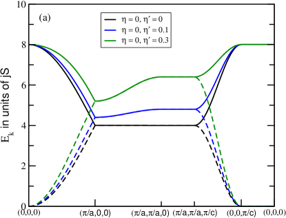
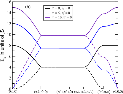
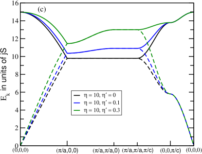
Figure 3: (Color online) (a) Magnon dispersion for acoustic (Goldstone) and optic magnons are shown for different values of intra-dimer coupling $\eta=J/j$ for NNN intra-bilayer ferromagnetic interaction $\eta^{\prime}=j^{\prime}/j=0$. (b, c) Effects of $\eta^{\prime}$ on the dispersion are for two different values of $\eta$. Each branch is two-fold degenerate corresponding to $\alpha$ and $\beta$ magnons.

Our tetragonal unit cell contains four Cr spins (two up and two down) – so there are two $\alpha$ and two $\beta$ branches for each ${\bf k}$. Fig. 3a displays the magnon dispersions for $\eta=0$, when the two bilayers are decoupled. In the decoupled bilayer limit there are two magnon modes ($\omega_{\bf k}^{(1)}$ and $\omega_{\bf k}^{(2)}$) with different dispersions corresponding to the two spins per the two-dimensional square lattice unit cell $[a{\hat{x}},a{\hat{y}}]$. If we compare this dispersion with the case of Cr₂TeO₆ (Fig. 2 of Ref. Majumdar and Mahanti, 2018) where the bilayers are antiferromagnetic, we find that the two modes are degenerate. In order to understand this we look at a smaller $2D$ unit cell, a rotated square lattice $[(a/2)({\hat{x}+\hat{y}}),(a/2)(-{\hat{x}}+{\hat{y}})]$ for which the corresponding BZ is larger. The dispersion for the ferro (F) case in the smaller unit cell when mapped into the smaller BZ of the larger unit cell, gives the two modes seen in Fig. 3a. On the other hand because of the degeneracy between $\alpha$ and $\beta$ for the antiferro (AF) case, the mapping gives a two-fold degenerate mode. When we turn on the inter-bilayer AF coupling the $\alpha$ and $\beta$ degeneracy does not split the two modes into four modes. If on the other hand, the inter-bilayer couplings were ferromagnetic one would have seen four modes corresponding to four ferromagnetically oriented spins per unit cell. The absence of $k_{z}$ dependence is obvious as with $\eta=0$ there is no coupling between the layers along the $z$-direction. Introduction of a nonzero NNN exchange coupling $\eta^{\prime}$ brings in dispersion along $(\pi/a,0,0)$ to $(\pi/a,\pi/a,0)$.

In Fig. 3b we show the effect of introducing inter-bilayer AF coupling $\eta$ (for simplicity we chose $\eta^{\prime}=0$). Non-zero $\eta$ couples the intra-bilayer modes, leading to acoustic (Goldstone modes, $\omega_{\bf k}^{(1)}\rightarrow 0$ as ${\bf k}\rightarrow 0$) and optic modes ($\omega_{\bf k}^{(2)}\rightarrow 4/\sqrt{4+\eta}$ as ${\bf k}\rightarrow 0$). The new $\alpha$ and $\beta$ modes are linear combinations of the old decoupled bilayer modes. The modes split into two modes along $(0,0,0)$ to $(\pi/a,0,0)$ and the zero frequency modes along $(0,0,0)$ to $(0,0,\pi/c)$ split into acoustic and optic modes. Interestingly, the modes along $(\pi/a,0,0)$ to $(\pi/a,\pi/a,0)$ to $(\pi/a,\pi/a,\pi/c)$ are dispersionless and four-fold degenerate. Finally, in Fig. 3c, we show how the NNN ferromagnetic coupling introduces dispersion to these modes, but it does not remove the degeneracy.

It is interesting to compare the basic differences in the magnon dispersions for the AF-AF and F-AF cases for the same value of $\eta\;(=10)$. For simplicity we again consider the case $\eta^{\prime}=0$. Comparing Fig. 3c of the present paper with Fig. 2c of Ref. Majumdar and Mahanti, 2018, we see that there is a strong similarity between the dispersions from $(0,0,0)\rightarrow(\pi/a,0,0)\rightarrow(\pi/a,\pi/a,0)\rightarrow(\pi/a,\pi/a,\pi/c)$, with the exception of the width of the optical magnons along $(0,0,0)\rightarrow(\pi/a,0,0)$. It is (in units of $jS$) about a factor of 2 larger for the F-AF case. The main difference is seen in the dispersions along $(0,0,0)\rightarrow(0,0,\pi/c)\rightarrow(\pi/a,\pi/a,\pi/c)$. Both the optic and acoustic branches are dramatically different.

As an example, consider the dispersions for the Goldstone mode for both F-AF and AF-AF (Ref. Majumdar and Mahanti, 2018) systems with non-zero small ${\bf k}$ (we kept $\eta^{\prime}=0$ for simplicity):

$$\omega_{\bf k}^{(1),{\rm F-AF}} \approx \Big{[}\frac{(k_{x}^{2}+k_{y}^{2})a^{2}}{4(\eta+4)^{2}}\Big{(}4\eta+(k_{x}^{2}+k_{y}^{2})a^{2}\Big{)}+\frac{\eta^{2}}{(4+\eta)^{3}}(k_{z}c)^{2}\Big{]}^{1/2},$$ (24a)

$$\omega_{\bf k}^{(1),{\rm AF-AF}} \approx \frac{1}{\sqrt{4+\eta}}\Big{[}(k_{x}^{2}+k_{y}^{2})a^{2}+\frac{\eta}{4+\eta}(k_{z}c)^{2}\Big{]}^{1/2}.$$ (24b)

For small $k_{x},k_{y}$ with $k_{z}=0$ (dispersion in the basal plane) $\omega_{\bf k}^{(1),{\rm F-AF}}\rightarrow\frac{ka}{2(4+\eta)}\sqrt{4\eta+(ka)^{2}}$ where $k=(k_{x}^{2}+k_{y}^{2})^{1/2}$. Clearly $\omega_{\bf k}^{(1),{\rm F-AF}}\rightarrow 0$ as $k\rightarrow 0$. For $ka<<\sqrt{4\eta}$, the dispersion is linear corresponding to AF magnons which behave like ferromagnetic magnons for $ka>>\sqrt{4\eta}$. The crossover occurs for the wave-vector $k_{c}\sim\sqrt{4\eta}/a$. As seen in Eq. (24a) a quadratic dispersion for $\eta=0$ starts to develop a linear term as $\eta$ becomes non-zero. We also note that for $k_{x}=k_{y}=0$ the dispersion is linear in $k_{z}$ with finite $\eta$ as seen in Fig. 3 for the region $(0,0,\pi/c)\rightarrow(0,0,0)$. This is in sharp contrast to the AF-AF system (Eq. (24b)) where a linear dispersion for $\eta=0$ remains linear when $\eta$ becomes finite (see Fig. 2b in Ref. Majumdar and Mahanti, 2018). Single crystal neutron scattering measurements should be able to detect these features.

II.2 Sublattice Magnetization

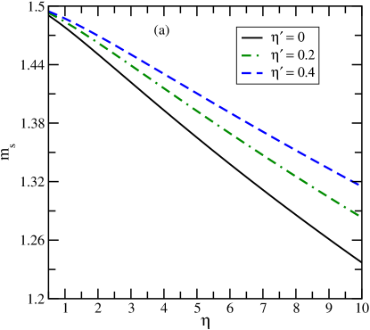
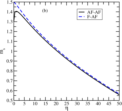
Figure 4: (Color online) (a) Normalized sublattice magnetization, $m_{s}$ is shown as a function of the inter-bilayer coupling parameter $\eta$ for different values of NNN interaction $\eta^{\prime}$. (b) Comparison of $m_{s}$ as a function of the inter-bilayer coupling parameter $\eta$ is shown for AF-AF and F-AF bilayers.

We calculate the normalized sublattice magnetization $m_{s}=M_{s}/M_{0}$ from Eq. (12) as a function of $\eta$. Fig. 4a shows the magnetizations for F-AF bilayer as a function of $\eta$ and for different values of $\eta^{\prime}$. For $\eta^{\prime}=0$, magnetization starts from the classical value 1.5 (at $\eta=0$) and then monotonically decreases with increasing $\eta$. This is expected as increasing antiferromagnetic coupling $\eta$ enhances QSF and thus reduces $m_{s}$. However, adding ferromagnetic NNN interactions $\eta^{\prime}$ enhances $m_{s}$ – this is shown in Fig. 4a for two different values of $\eta^{\prime}=0.2$ and $0.4$. On the other hand for AF-AF bilayer (as in Cr₂TeO₆ systems) $m_{s}$ increases from the initial value of 1.303 (at $\eta=\eta^{\prime}=0$) to 1.406 (at $\eta=1.25$) and then decreases monotonically as shown in Fig. 4b. Eventually for large value of $\eta$, $m_{s}$ for both AF-AF and F-AF bilayer approach each other.

II.3 Two-Magnon Density of States (TM-DOS)

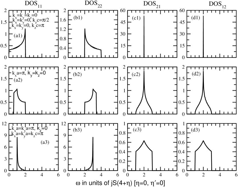
Figure 5: (a1–d3) Two-magnon density of states for different values of ${\bf k}$ is plotted for $\eta=\eta^{\prime}=0$. Notice that DOS${}_{12}({\bf k},\omega)=$DOS${}_{21}({\bf k},\omega)$.

The longitudinal spin-spin correlation function ${\cal L}_{s}({\bf k},\omega)$, which is directly probed in inelastic scattering measurements depends sensitively on TM-DOS. The latter are calculated for different ${\bf k}$-values by numerically evaluating the internal three-dimensional momenta ${\bf p}$ on a mesh grid of size $L\times L\times L$, where $L=256$. A Gaussian function of width $\sigma=0.075$ (in units of frequency $\omega$) is used to broaden the $\delta$-function. In Fig. 5, we present all four two-magnon DOS$({\bf k},\omega)$ for $\eta=0$. As discussed earlier, in the absence of inter-bilayer coupling one has ferromagnetic magnons associated with the two branches of the dispersion shown in Fig. 3a. Although the two intra-mode TM-DOS, DOS${}_{11}({\bf k},\omega)$ and DOS${}_{22}({\bf k},\omega)$ are different, the two inter-mode TM-DOS, DOS${}_{21}({\bf k},\omega)$ and DOS${}_{12}({\bf k},\omega)$ are equal.

Next, we discuss the case when inter-bilayer coupling is nonzero ($\eta\neq 0$). Since in the Cr₂(W, Mo)O₆ systems, $|J|$ is much larger than the intra-bilayer coupling $|j|$ we choose $\eta=10$ and still keep $\eta^{\prime}=0$ for simplicity. In Fig. 6 and Fig. 7, we plot the $({\bf k},\omega)$ dependence of DOS₁₁, DOS₂₂, DOS₂₁, and DOS₁₂. The equality ${\rm DOS}_{12}({\bf k},\omega)={\rm DOS}_{21}({\bf k},\omega)$ for any ${\bf k}$ is still preserved for non-zero $\eta$.

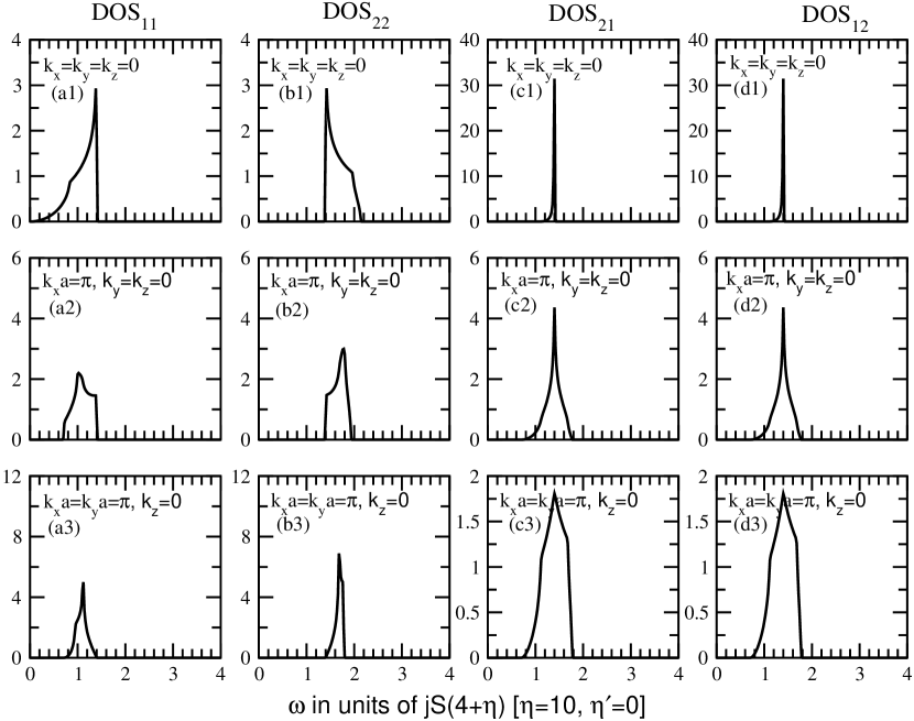
Figure 6: (a1–d3) Two-magnon DOS for different values of $(k_{x},k_{y})$ with $k_{z}=0$ is plotted for $\eta=10,\eta^{\prime}=0$. Notice that the symmetry DOS${}_{12}({\bf k},\omega)=$DOS${}_{21}({\bf k},\omega)$ still persists even for non-zero $\eta$.

In Fig. 6, we choose $k_{z}=0$ and study the $(k_{x},k_{y})$ dependence and in Fig. 7, we show the effect of $k_{z}$ on all four TM-DOS. Consider the evolution of the four TM-DOS as a function of $k_{z}$ with $k_{x}=k_{y}=0$ as shown in Fig. 6a1-d1, Fig. 7a1-d1, and Fig. 7a2-d2. Especially consider the peak intensity (at 19.6$jS$) for the inter-band density of states DOS₁₂ (=DOS₂₁). The intensity is $\sim 32$ for $k_{x}=k_{y}=k_{z}=0$ [Fig. 6c1] whereas it decreases to $\sim 15$ (at 19.6$jS$) for $k_{x}=k_{y}=0,k_{z}=\pi$ [Fig. 7c1]. Interestingly there is no change in the peak intensity for DOS₁₁ and DOS₂₂ [Fig. 7a1-b1].

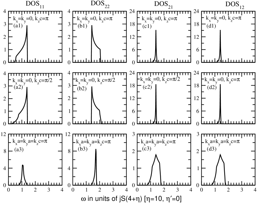
Figure 7: (a1–d3) Two-magnon DOS for different values of $(k_{x},k_{y},k_{z})$ is plotted for $\eta=10,\eta^{\prime}=0$. The plots show the $k_{z}$ dependence on the four DOS.

II.4 Longitudinal spin-spin correlation function (LSSCF)

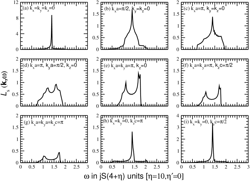
Figure 8: (a–i) Longitudinal spin-spin correlation, ${\cal L}_{s}({\bf k},\omega)$ for different values of ${\bf k}$ is plotted for $\eta=10,\eta^{\prime}=0$.

In Fig. 8a-i, we show the ${\bf k}$-dependence of LSSCF ${\cal L}_{s}({\bf k},\omega)$. As seen in Eq. (20), contributions from different two-magnon excitations get weighted by the associated weights ${\cal D}^{ij}_{{\bf k},{\bf k+p}}$. This leads to different energy dependence of LSSCF compared to that of the total two-magnon DOS. In Fig. 9 we show both ${\cal L}_{s}({\bf k},\omega)$ and the sum of the four DOS${}_{ij}({\bf k},\omega)$ for ${\bf k}=0$ and $k_{x}a=k_{y}a=k_{z}c=\pi$. Both ${\cal L}_{s}({\bf k},\omega)$ and $\sum$DOS${}_{ij}({\bf k},\omega)$ show similar features. However the intensity of the peak in ${\cal L}_{s}({\bf k},\omega)$ is reduced significantly, which shows the effect of the weights. Another interesting feature is that ${\cal L}_{s}({\bf k},\omega)$ has only one peak at $\omega=1.4jS(4+\eta)=19.5jS$ for ${\bf k}=0$ [Fig. 8a], whereas for $k_{x}a=k_{y}a=k_{z}c=\pi$ two peaks emerge, one at $\omega=1.0jS(4+\eta)=14.6jS$ and the other at $\omega=1.74jS(4+\eta)=24.4jS$ [Fig. 8g]. The formation of two peaks from a single peak in ${\cal L}_{s}({\bf k},\omega)$ can be seen in Fig. 8.

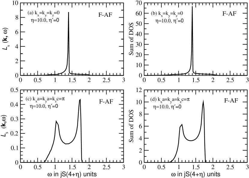
Figure 9: (a – d) Longitudinal spin-spin correlation ${\cal L}_{s}({\bf k},\omega)$ and the sum of the density of states of four magnon branches are plotted for $\eta=10.0,\eta^{\prime}=0$ or two different values of ${\bf k}$. The plots show the effect of the weights ${\cal D}_{ij}$ in ${\cal L}_{s}({\bf k},\omega)$.

Finally, we plot the angular average of ${\cal L}_{s}({\bf k},\omega)$ for different magnitudes of $|{\bf k}|=Q$ in Fig. 10. For these plots, Eq. (23) was numerically evaluated by summing over the angles $\theta,\phi$. For each $\omega$ about 270 million points were evaluated. This is what can be observed in a inelastic neutron scattering experiment from a powder sample. The generic feature is a narrow peak seen at $\sim 19.5jS$ with two broad peaks on each side. With increase in the magnitude of ${\bf k}$ the intensity initially decreases (from $Qa=0$ to $Qa=0.50\pi$) and then increases (from $Qa=\pi$ to $Qa=1.5\pi$). Moreover the broad peak at $\omega=2.0jS(4+\eta)=28jS$ increases in intensity with increase in $Q$.

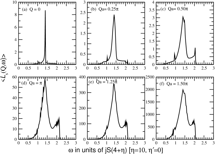
Figure 10: (a – f) Powder-averaged longitudinal spin-spin correlation function $\langle{\cal L}_{s}(|{\bf k}|=Q,\omega)\rangle$ for $\eta=10,\eta^{\prime}=0$ and $Qa=0,0.25\pi,0.5\pi,\pi$.

III Comparison between F-AF and AF-AF bilayer systems

In our previous work we studied the low-temperature magnetic properties of the Cr₂TeO₆ bilayer system where both the intra and inter-bilayer couplings are antiferromagnetic. Majumdar and Mahanti (2018) In this paper we have discussed the magnon dispersion, two-magnon density of states, and longitudinal spin-spin correlation function in the leading order approximation for Cr₂WO₆ and Cr₂MoO₆ coupled bilayer systems where inter-bilayer NN coupling is antiferromagnetic but intra-bilayer coupling is ferromagnetic. We have also investigated how a small intra-bilayer NNN ferromagnetic coupling affects the above properties.

We find that F-AF system differs in several ways from the AF-AF system studied in the earlier paper. Majumdar and Mahanti (2018)

1. For the F-AF bilayer system the two magnon branches with frequencies $\omega_{\bf k}^{(1)}$ and $\omega_{\bf k}^{(2)}$ corresponding to two bilayers for $\eta=0$ are non-degenerate [Fig. 3] except between $(\pi/a,0,0)$ to $(\pi/a,\pi/a,0)$ to $(\pi/a,\pi/a,\pi/c)$ (within LSWT - higher order $1/S$ corrections may lift this degeneracy). This result is different from the AF-AF case (for Cr₂TeO₆ systems) where both the branches are degenerate throughout the first BZ [Fig. 2 of Ref. Majumdar and Mahanti, 2018]. Also as we pointed out earlier, for large values of $\eta(=10)$, the magnon dispersions are very similar along $(0,0,0)\rightarrow(\pi/a,0,0)\rightarrow(\pi/a,\pi/a,0)\rightarrow(\pi/a,\pi/a,\pi/c)$ for the two cases, but differ dramatically from $(0,0,0)\rightarrow(0,0,\pi/c)\rightarrow(\pi/a,\pi/a,\pi/c)$.

   As another example, the dispersions for the Goldstone mode between F-AF and AF-AF systems are quite different as seen in Eqs. (24a)-(24b). For the F-AF system a quadratic dispersion for $\eta=0$ starts to develop a linear term as $\eta$ becomes non-zero (see Eq. (24a)) whereas for the AF-AF system a linear dispersion for $\eta=0$ remains linear when $\eta$ becomes finite (see Eq. (24b)).

2. The normalized sublattice magnetization $m_{s}$ for both F-AF and AF-AF bilayer systems differs substantially from its classical value due to quantum spin fluctuations with increase in $\eta$ [Fig. 4b]. In case of F-AF bilayers $m_{s}$ start from the classical value of 1.5 (at $\eta=0$) and then monotonically decreases with increasing $\eta$. On the contrary, for the AF-AF bilayer system, we have found a non-monotonic $\eta$ dependence of $m_{s}$ – it initially increases from the initial value of 1.303 at $\eta=\eta^{\prime}=0$ to 1.406 (at $\eta=1.25$) and then decreases monotonically. Eventually for large values of $\eta$, $m_{s}$ for both AF-AF and F-AF bilayers become identical. Addition of ferromagnetic NNN interaction $j^{\prime}$ suppresses QSF effects and thereby enhances $m_{s}$ in both cases.

   

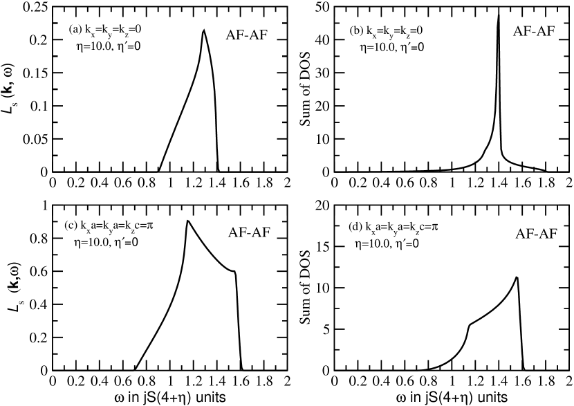
   Figure 11: Longitudinal spin-spin correlation ${\cal L}_{s}({\bf k},\omega)$ and the sum of the density of states of four magnon branches are plotted for $\eta=10.0,\eta^{\prime}=0$ or two different values of ${\bf k}$ for the AF-AF system. The plots show the effect of the weights ${\cal D}_{ij}$ in ${\cal L}_{s}({\bf k},\omega)$.

3. There are some differences for the two-magnon DOS between AF-AF and F-AF bilayer systems with $\eta=10,\eta^{\prime}=0$ [Fig. 6-7 and Figs. 5 and 6 in Ref. Majumdar and Mahanti, 2018]. As an example, for ${\bf k}=0$, DOS₁₂=DOS₂₁ for both the systems. But for $k_{x}=k_{y}=0,k_{z}c=\pi$, two inter-band DOS are equal to their corresponding two intra-band DOS i.e. DOS₁₁=DOS₁₂ and DOS₂₂=DOS₂₁ for AF-AF bilayers whereas for F-AF bilayers only the two inter-band DOS are equal, i.e. DOS₁₂=DOS₂₁. Another interesting observation is that for the AF-AF bilayers ${\cal L}_{s}({\bf k},\omega)=0$ at $k_{x}a=k_{y}a=\pi,k_{z}=0$ even though all the density of states are non-zero [Fig. 7e in Ref. Majumdar and Mahanti, 2018]. But with the F-AF bilayers, we have not found any ${\bf k}$ for which ${\cal L}_{s}({\bf k},\omega)$ vanishes with non-zero DOS.

4. Comparison of the sum of the density of states (right panel) with LSSCF (left panel) in Figs. 9 and 11 show the effect of the wave-functions on ${\cal L}_{s}({\bf k},\omega)$. We observe from Fig. 11 that for the AF-AF system the wave-functions substantially changes the LSSCF structure from the sum of DOS. On the contrary, for the F-AF system in Fig. 9 the change in the structure of LSSCF from the sum of DOS is minimal (other than an overall reduction in the peak intensity).

5. Finally for the powder average we find only a narrow peak seen at $19.5jS$ [at $\omega=1.4jS(4+\eta)$] with a small broad peak at lower energies for the AF-AF system [Fig. 9 of Ref. Majumdar and Mahanti, 2018]. But, for the F-AF system a narrow peak is seen at $\sim 19.5jS$ [at $\omega=1.4jS(4+\eta)$] with two broad peaks on each side [Fig. 10(c–f)]. However the broad peak at $\sim 28jS$ [at $\omega=2jS(4+\eta)$] increases in intensity with increase in $|k|=Q$. One more difference is that for the AF-AF system the intensity increases with increase in the magnitude of ${\bf k}$, whereas for the F-AF system it first decreases and then increases as we approach the zone boundary at $Q=1.5\pi/a$.

IV Conclusions

In this article we studied the magnetic properties (magnon dispersion, suppression of long range order by quantum spin fluctuation, two-magnon density of states, longitudinal spin-spin correlation function and its angular average) of Cr₂WO₆ and Cr₂MO₆, which are bilayer systems of antiferromagnetically coupled (strength $J$) quantum spin-3/2 dimers interacting through $2D$ ferromagnetic coupling (strength $j$). In addition to $J$ and $j$, there is also a small inter-dimer longer range ferromagnetic coupling ($j^{\prime}$) whose magnitude is much smaller than $J$ and $j$. For convenience we will consider $j^{\prime}=0$. In a recent paper [Ref. Majumdar and Mahanti, 2018], we discussed the magnetic properties of a related system, Cr₂TeO₆, where the dimers are coupled antiferromagnetically. There are many similarities and differences between the two cases (F-AF and AF-AF). In the limit $J=0$, W and Mo systems reduce to non-interacting $2D$ ferromagnetic (F) sheets whereas the Te system reduces to non-interacting $2D$ antiferromagnetic (AF) sheets. The magnon dispersions are therefore qualitatively different, for small ${\bf k}$ (linear for AF and quadratic for F sheets). In addition the total magnon band-width (in unit of $j$S) is 4 for AF and 8 for F. However, the intra-dimer AF coupling is dominant, $J\sim 10j$, and it controls the magnon dispersion. In this limit, magnon dispersions are qualitatively similar excepting along the directions $(0,0,0)$ to $(0,0,\pi/c)$ and along $(0,0,\pi/c)$ to $(\pi/a,\pi/a,\pi/c)$ (see Fig. 2(c) of Ref. Majumdar and Mahanti, 2018 and Fig. 3c of this paper, for $\eta^{\prime}=0$). In the case of intra-layer AF coupling, the inter-layer AF coupling introduces two magnon modes (acoustic and optic) propagating along the $c$-axis which become degenerate at $(0,0,\pi/c)$. In contrast, for intra-layer F coupling, there is a large gap between the acoustic and optic modes $(\sim 7jS)$ at $(0,0,\pi/c)$. Careful single-crystal inelastic neutron scattering measurements should be able to detect these subtle differences between the Te system and W/Mo system. Quantum spin fluctuations (QSF) suppress the ordered maagnetization $(M_{s}/M_{0})$ from its classical value $3/2$ for both F-AF and AF-AF systems. In W/Mo systems, $(M_{s}/M_{0})$ reduces monotonically from the classical value as $\eta$ increases. On the other hand, for the Te case, QSF already reduce $(M_{s}/M_{0})$ when $\eta=0$. Introduction of $\eta$ first suppresses QSF and enhances the magnetization and then for larger $\eta$ values it decreases monotonically similar to the F-AF system. In case of F-AF system for $\eta=10$, $M_{s}/M_{0}\sim 1.23-1.25$, which is about 17-18% reduction (see Fig. 4b). Finally for the angle averaged longitudinal spin-spin correlation function $\langle{\cal L}_{s}(Q,\omega)\rangle$ the scattering intensity is a factor of 10 stronger for the W/Mo system compared to the Te system, again a result which can be verified experimentally.

V Acknowledgment

We acknowledge the use of HPC cluster at GVSU, supported by the National Science Foundation Grant No. CNS-1228291 that have contributed to the research results reported within this paper. SDM would like to thank Dr. Xianglin Ke for stimulating discussions.

Appendix A Brief derivation of the Hamiltonian in momentum space

The spin Hamiltonian in Eq. (2) is mapped onto a Hamiltonian of interacting bosons by expressing the spin operators in terms of bosonic creation and annihilation operators $a^{\dagger},a$ for “up” sites on sublattice A (and $b^{\dagger},b$ for “down” sites on sublattice B) using the Holstein-Primakoff representation Holstein and Primakoff (1940)

$$S_{in}^{+A} \approx \sqrt{2S}a_{in},\;\;\;S_{in}^{-A}\approx\sqrt{2S}a_{in}^{\dagger},\;\;\;S_{in}^{zA}=S-a^{\dagger}_{in}a_{in},$$ (25a)

$$S_{jn}^{+B} \approx \sqrt{2S}b_{jn}^{\dagger},\;\;\;S_{jn}^{-B}\approx\sqrt{2S}b_{jn},\;\;\;S_{jn}^{zB}=-S+b^{\dagger}_{jn}b_{jn}.$$ (25b)

After substituting Eqs. (25) into Eq. (2) and expanding the Hamiltonian perturbatively in powers of $1/S$ (up to the quadratic term) we obtain:

$${\cal H}={\cal H}_{\rm cl}+{\cal H}_{0}+\cdots,$$ (26)

where,

$${\cal H}_{\rm cl} = -2jNS^{2}(4+\eta),$$ (27a)

$${\cal H}_{0} = jS\sum_{n=1}^{N_{z}}\sum_{\langle i,j\rangle}\Big{[}a_{in}^{(1)\dagger}a_{in}^{(1)}+a_{in}^{(2)\dagger}a_{in}^{(2)}+b_{jn}^{(3)\dagger}b_{jn}^{(3)}+b_{jn}^{(4)\dagger}b_{jn}^{(4)}$$ (27b)

$$- a_{in}^{(1)}a_{jn}^{(2)\dagger}-a_{in}^{(1)\dagger}a_{jn}^{(2)}-b_{in}^{(3)\dagger}b_{jn}^{(4)}-b_{in}^{(3)}b_{jn}^{(4)\dagger}\Big{]}$$

$$+ JS\sum_{n=1}^{N_{z}}\sum_{i}\Big{[}a_{in}^{(1)\dagger}a_{in}^{(1)}+b_{in}^{(3)\dagger}b_{in}^{(3)}+a_{in}^{(1)}b_{in}^{(3)}+a_{in}^{(1)\dagger}b_{in}^{(3)\dagger}$$

$$+ \frac{1}{2}\Big{\{}a_{in}^{(2)\dagger}a_{in}^{(2)}+a_{in+1}^{(2)\dagger}a_{in+1}^{(2)}+b_{in}^{(4)\dagger}b_{in}^{(4)}+b_{in-1}^{(4)\dagger}b_{in-1}^{(4)}$$

$$+ a_{in}^{(2)}b_{in-1}^{(4)}+a_{in}^{(2)\dagger}b_{in-1}^{(4)\dagger}+a_{in+1}^{(2)}b_{in}^{(4)}+a_{in+1}^{(2)\dagger}b_{in}^{(4)\dagger}\Big{\}}\Big{]}$$

$$+ j^{\prime}S\sum_{n=1}^{N_{z}}\sum_{\langle\langle i,j\rangle\rangle}\sum_{p=1,2}\Big{[}a_{in}^{(p)\dagger}a_{in}^{(p)}+a_{jn}^{(p)\dagger}a_{jn}^{(p)}-a_{in}^{(p)\dagger}a_{jn}^{(p)}-a_{in}^{(p)}a_{jn}^{(p)\dagger}\Big{]}$$

$$+ j^{\prime}S\sum_{n=1}^{N_{z}}\sum_{\langle\langle i,j\rangle\rangle}\sum_{p=3,4}\Big{[}b_{in}^{(p)\dagger}b_{in}^{(p)}+b_{jn}^{(p)\dagger}b_{jn}^{(p)}-b_{in}^{(p)\dagger}b_{jn}^{(p)}-b_{in}^{(p)}b_{jn}^{(p)\dagger}\Big{]}.$$

${\cal H}_{\rm cl}$ represents the classical ground state (mean-field) energy and it is not relevant for the quantum fluctuations, so we do not discuss it further. $H_{0}$ in Eq. (27b) is the quadratic part of the Hamiltonian. In Eq. (27a), the parameters $\eta=J/j$, $\eta^{\prime}=j^{\prime}/j$ and $N=N_{x}N_{y}N_{z}$ is the total number of unit cells. Next the real space Hamiltonian is transformed to momentum space using the Fourier transformation for each $\ell$-th spin:

$$a_{in}^{(\ell)}=\frac{1}{\sqrt{N}}\sum_{{\bf k}}e^{i{\bf k\cdot R_{in}^{(\ell)}}}a_{\bf k}^{(\ell)},\;\;\;b_{in}^{(\ell)}=\frac{1}{\sqrt{N}}\sum_{{\bf k}}e^{-i{\bf k\cdot R_{in}^{(\ell)}}}b_{-\bf k}^{(\ell)}.$$ (28)

Furthermore we have rescaled the operators $a,\;b$ as

$$a_{\bf k}^{(1)} \equiv e^{-ik_{z}\delta/2}a_{\bf k}^{(1)},\;\;a_{\bf k}^{(4)}\equiv e^{-ik_{z}\delta/2}a_{\bf k}^{(4)},$$

$$b_{-\bf k}^{(2)} \equiv e^{-ik_{z}\delta/2}b_{-\bf k}^{(2)},\;\;b_{-\bf k}^{(3)}\equiv e^{-ik_{z}\delta/2}b_{-\bf k}^{(3)},$$

where $\delta$ is the inter-dimer separation (Fig. 1). In momentum space the quadratic Hamiltonian is shown in Eq. (3).

Appendix B Coefficients for Bogoliubov transformation

First we define the following functions:

$$U_{1\bf k} = -(1+\omega_{\bf k}^{(1)})(1+|\gamma_{1\bf k}|^{2}-\gamma_{2\bf k}^{2}-\omega^{(1)2}_{\bf k})+2|\gamma_{1\bf k}|^{2},$$ (29a)

$$U_{1\bf k}^{\prime} = -(1+\omega_{\bf k}^{(2)})(1+|\gamma_{1\bf k}|^{2}-\gamma_{2\bf k}^{2}-\omega^{(2)2}_{\bf k})+2|\gamma_{1\bf k}|^{2},$$ (29b)

$$U_{2\bf k} = -\gamma_{1\bf k}[(1+\omega_{\bf k}^{(1)})^{2}-|\gamma_{1\bf k}|^{2}]-\gamma_{1\bf k}^{*}\gamma_{2\bf k}^{2},$$ (29c)

$$U_{2\bf k}^{\prime} = -\gamma_{1\bf k}[(1+\omega_{\bf k}^{(2)})^{2}-|\gamma_{1\bf k}|^{2}]-\gamma_{1\bf k}^{*}\gamma_{2\bf k}^{2},$$ (29d)

$$V_{1\bf k} = (\gamma_{1\bf k}+\gamma_{1\bf k}^{*})\gamma_{2\bf k}+\omega_{\bf k}^{(1)}(\gamma_{1\bf k}-\gamma_{1\bf k}^{*})\gamma_{2\bf k},$$ (29e)

$$V_{1\bf k}^{\prime} = (\gamma_{1\bf k}+\gamma_{1\bf k}^{*})\gamma_{2\bf k})+\omega_{\bf k}^{(2)}(\gamma_{1\bf k}-\gamma_{1\bf k}^{*})\gamma_{2\bf k},$$ (29f)

$$V_{2\bf k} = \gamma_{2\bf k}(1-\gamma_{2\bf k}^{2}-\omega^{(1)2}_{\bf k})+\gamma_{1\bf k}^{2}\gamma_{2\bf k},$$ (29g)

$$V_{2\bf k}^{\prime} = \gamma_{2\bf k}(1-\gamma_{2\bf k}^{2}-\omega^{(2)2}_{\bf k})+\gamma_{1\bf k}^{2}\gamma_{2\bf k},$$ (29h)

then the coefficients for the BG transformaitons are –

$$\ell_{1\bf k} = U_{1\bf k}/N_{1\bf k},\;\;\ell_{1\bf k}^{\prime}=U_{1\bf k}^{\prime}/N_{2\bf k},\;\;\ell_{2\bf k}=U_{2\bf k}/N_{1\bf k},\;\;\ell_{2\bf k}^{\prime}=U_{2\bf k}^{\prime}/N_{2\bf k},$$ (30a)

$$m_{1\bf k} = V_{1\bf k}/N_{1\bf k},\;\;m_{1\bf k}^{\prime}=V_{1\bf k}^{\prime}/N_{2\bf k},\;\;m_{2\bf k}=V_{2\bf k}/N_{1\bf k},\;\;m_{2\bf k}^{\prime}=V_{2\bf k}^{\prime}/N_{2\bf k},$$ (30b)

where the normalization factors $N_{1\bf k},N_{2\bf k}$ are given by:

$$N_{1\bf k} = \Big{[}|U_{1\bf k}|^{2}-|V_{1\bf k}|^{2}+|U_{2\bf k}|^{2}-|V_{2\bf k}|^{2}\Big{]}^{1/2},$$ (31a)

$$N_{2\bf k} = \Big{[}|U_{1\bf k}^{\prime}|^{2}-|V_{1\bf k}^{\prime}|^{2}+|U_{2\bf k}^{\prime}|^{2}-|V_{2\bf k}^{\prime}|^{2}\Big{]}^{1/2}.$$ (31b)

Appendix C Total spin $S_{z}$ in terms of $\alpha$ and $\beta$ magnons

$$S_{z}({\bf k}) = -\frac{1}{\sqrt{4N}}\sum_{{\bf p,q}}\delta({\bf k}+{\bf p}-{\bf q})$$ (32)

$$\Big{[} \{[f_{1{\bf k}}\ell_{1\bf p}^{*}\ell_{1\bf q}+f_{2{\bf k}}\ell^{\prime*}_{2\bf p}\ell^{\prime}_{2\bf q}]-[f_{3{\bf k}}m^{\prime}_{2{\bf q}}m^{\prime*}_{2{\bf p}}+f_{4{\bf k}}m_{1{\bf q}}m^{*}_{1{\bf p}}]\}\alpha_{\bf p}^{(1)\dagger}\alpha_{\bf q}^{(1)}$$

$$+ \{[f_{1{\bf k}}\ell_{1\bf p}^{\prime*}\ell_{1\bf q}^{\prime}+f_{2{\bf k}}\ell^{*}_{2\bf p}\ell_{2\bf q}]-[f_{3{\bf k}}m_{2{\bf q}}m^{*}_{2{\bf p}}+f_{4{\bf k}}m_{1{\bf q}}^{\prime}m^{\prime*}_{1{\bf p}}]\}\alpha_{\bf p}^{(2)\dagger}\alpha_{\bf q}^{(2)}$$

$$+ \{[f_{1{\bf k}}m_{1\bf p}^{*}m_{1\bf q}+f_{2{\bf k}}m^{\prime*}_{2\bf p}m^{\prime}_{2\bf q}]-[f_{3{\bf k}}\ell^{\prime}_{2{\bf q}}\ell^{\prime*}_{2{\bf p}}+f_{4{\bf k}}\ell_{1{\bf q}}\ell^{*}_{1{\bf p}}]\}\beta_{-\bf q}^{(1)\dagger}\beta_{-\bf p}^{(1)}$$

$$+ \{[f_{1{\bf k}}m_{1\bf p}^{\prime*}m_{1\bf q}^{\prime}+f_{2{\bf k}}m^{*}_{2\bf p}m_{2\bf q}]-[f_{3{\bf k}}\ell_{2{\bf q}}\ell^{*}_{2{\bf p}}+f_{4{\bf k}}\ell_{1{\bf q}}^{\prime}\ell^{\prime*}_{1{\bf p}}]\}\beta_{-\bf q}^{(2)\dagger}\beta_{-\bf p}^{(2)}$$

$$+ \{[f_{1{\bf k}}\ell_{1\bf p}^{*}m_{1\bf q}+f_{2{\bf k}}\ell^{\prime*}_{2\bf p}m^{\prime}_{2\bf q}]-[f_{3{\bf k}}\ell^{\prime}_{2{\bf q}}m^{\prime*}_{2{\bf p}}+f_{4{\bf k}}\ell_{1{\bf q}}m^{*}_{1{\bf p}}]\}\alpha_{\bf p}^{(1)\dagger}\beta_{-\bf q}^{(1)\dagger}$$

$$+ \{[f_{1{\bf k}}m_{1\bf p}^{*}\ell_{1\bf q}+f_{2{\bf k}}m^{\prime*}_{2\bf p}\ell^{\prime}_{2\bf q}]-[f_{3{\bf k}}m^{\prime}_{2{\bf q}}\ell^{\prime*}_{2{\bf p}}+f_{4{\bf k}}m_{1{\bf q}}\ell^{*}_{1{\bf p}}]\}\alpha_{\bf q}^{(1)}\beta_{-\bf p}^{(1)}$$

$$+ \{[f_{1{\bf k}}\ell_{1\bf p}^{\prime*}m_{1\bf q}^{\prime}+f_{2{\bf k}}\ell^{*}_{2\bf p}m_{2\bf q}]-[f_{3{\bf k}}\ell_{2{\bf q}}m^{*}_{2{\bf p}}+f_{4{\bf k}}\ell_{1{\bf q}}^{\prime}m^{\prime*}_{1{\bf p}}]\}\alpha_{\bf p}^{(2)\dagger}\beta_{\bf q}^{(2)\dagger}$$

$$+ \{[f_{1{\bf k}}m_{1\bf p}^{\prime*}\ell_{1\bf q}^{\prime}+f_{2{\bf k}}m^{*}_{2\bf p}\ell_{2\bf q}]-[f_{3{\bf k}}m_{2{\bf q}}\ell^{*}_{2{\bf p}}+f_{4{\bf k}}m_{1{\bf q}}^{\prime}\ell^{\prime*}_{1{\bf p}}]\}\alpha_{\bf q}^{(2)}\beta_{-\bf p}^{(2)}$$

$$+ \{[f_{1{\bf k}}\ell_{1\bf p}^{*}\ell_{1\bf q}^{\prime}+f_{2{\bf k}}\ell^{\prime*}_{2\bf p}\ell_{2\bf q}]-[f_{3{\bf k}}m_{2{\bf q}}m^{\prime*}_{2{\bf p}}+f_{4{\bf k}}m_{1{\bf q}}^{\prime}m^{*}_{1{\bf p}}]\}\alpha_{\bf p}^{(1)\dagger}\alpha_{\bf q}^{(2)}$$

$$+ \{[f_{1{\bf k}}\ell_{1\bf p}^{\prime*}\ell_{1\bf q}+f_{2{\bf k}}\ell^{*}_{2\bf p}\ell_{2\bf q}^{\prime}]-[f_{3{\bf k}}m_{2{\bf q}}^{\prime}m^{*}_{2{\bf p}}+f_{4{\bf k}}m_{1{\bf q}}m^{\prime*}_{1{\bf p}}]\}\alpha_{\bf p}^{(2)\dagger}\alpha_{\bf q}^{(1)}$$

$$+ \{[f_{1{\bf k}}\ell_{1\bf p}^{*}m_{1\bf q}+f_{2{\bf k}}\ell^{\prime*}_{2\bf p}m_{2\bf q}]-[f_{3{\bf k}}\ell_{2{\bf q}}m^{\prime*}_{2{\bf p}}+f_{4{\bf k}}\ell_{1{\bf q}}^{\prime}m^{*}_{1{\bf p}}]\}\alpha_{\bf p}^{(1)\dagger}\beta_{-\bf q}^{(2)\dagger}$$

$$+ \{[f_{1{\bf k}}m_{1\bf p}^{\prime*}\ell_{1\bf q}+f_{2{\bf k}}m^{*}_{2\bf p}\ell^{\prime}_{2\bf q}]-[f_{3{\bf k}}m^{\prime}_{2{\bf q}}\ell^{*}_{2{\bf p}}+f_{4{\bf k}}m_{1{\bf q}}\ell^{\prime*}_{1{\bf p}}]\}\alpha_{\bf q}^{(1)}\beta_{-\bf p}^{(2)}$$

$$+ \{[f_{1{\bf k}}\ell_{1\bf p}^{\prime*}m_{1\bf q}+f_{2{\bf k}}\ell^{*}_{2\bf p}m^{\prime}_{2\bf q}]-[f_{3{\bf k}}\ell^{\prime}_{2{\bf q}}m^{\prime}_{2{\bf p}}+f_{4{\bf k}}\ell_{1{\bf q}}m^{\prime*}_{1{\bf p}}]\}\alpha_{\bf p}^{(2)\dagger}\beta_{-\bf q}^{(1)\dagger}$$

$$+ \{[f_{1{\bf k}}m_{1\bf p}^{*}\ell_{1\bf q}^{\prime}+f_{2{\bf k}}m^{*}_{2\bf p}\ell_{2\bf q}]-[f_{3{\bf k}}m_{2{\bf q}}\ell^{\prime*}_{2{\bf p}}+f_{4{\bf k}}m_{1{\bf q}}^{\prime}\ell^{*}_{1{\bf p}}]\}\alpha_{\bf q}^{(2)}\beta_{-\bf p}^{(1)}$$

$$+ \{[f_{1{\bf k}}m_{1\bf p}^{*}m_{1\bf q}^{\prime}+f_{2{\bf k}}m^{\prime*}_{2\bf p}m_{2\bf q}]-[f_{3{\bf k}}\ell_{2{\bf q}}\ell^{\prime*}_{2{\bf p}}+f_{4{\bf k}}\ell_{1{\bf q}}^{\prime}\ell^{*}_{1{\bf p}}]\}\beta_{-\bf p}^{(1)}\beta_{-\bf q}^{(2)\dagger}$$

$$+ \{[f_{1{\bf k}}m_{1\bf p}^{\prime*}m_{1\bf q}+f_{2{\bf k}}m^{\prime*}_{2\bf p}m_{2\bf q}^{\prime}]-[f_{3{\bf k}}\ell_{2{\bf q}}^{\prime}\ell^{*}_{2{\bf p}}+f_{4{\bf k}}\ell_{1{\bf q}}\ell^{\prime*}_{1{\bf p}}]\}\beta_{-\bf p}^{(2)}\beta_{-\bf q}^{(1)\dagger}\Big{]}.$$

References

- Anderson (1952) P. W. Anderson, Phys. Rev. 86, 694 (1952).
- Harris et al. (1971) A. B. Harris, D. Kumar, B. I. Halperin, and P. C. Hohenberg, Phys. Rev. B 3, 961 (1971).
- Diep (2004) H. T. Diep, Frustrated Spin Systems, 1st ed. (World Scientific, Singapore, 2004).
- Lacroix et al. (2011) C. Lacroix, P. Mendels, and F. Mila, Introduction to Frustrated Magnetism, 1st ed., Vol. 164 (Springer-Verlag, Berlin, 2011).
- Rastelli (2013) E. Rastelli, Statistical Mechanics of Magnetic Excitations, 1st ed., Vol. 18 (World Scientific, Singapore, 2013).
- Majumdar (2010) K. Majumdar, Phys. Rev. B 82, 144407 (2010).
- Majumdar (2011a) K. Majumdar, J. Phys.: Condens. Matter 23, 046001 (2011a).
- Majumdar (2011b) K. Majumdar, J. Phys.: Condens. Matter 23, 116004 (2011b).
- Majumdar et al. (2012) K. Majumdar, D. Furton, and G. S. Uhrig, Phys. Rev. B 85, 144420 (2012).
- Uhrig and Majumdar (2013) G. S. Uhrig and K. Majumdar, Eur. Phys. J. B86, 282 (2013).
- Sachdev (2001) S. Sachdev, Quantum Phase Transitions, 1st ed. (Cambridge University Press, Cambridge, UK, 2001).
- Zhu et al. (2014) M. Zhu, D. Do, C. R. DelaCruz, Z. Dun, H. D. Zhou, S. D. Mahanti, and X. Ke, Phys. Rev. Lett. 113, 076406 (2014).
- Mahanti and Kaplan (1991) S. D. Mahanti and T. A. Kaplan, J. Appl. Phys. 69, 5382 (1991).
- Zhu et al. (2015) M. Zhu, D. Do, C. R. DelaCruz, Z. Dun, J. G. Cheng, H. Goto, Y. Uwatoko, T. Zou, H. D. Zhou, S. D. Mahanti, and X. Ke, Phys. Rev. B 92, 094419 (2015).
- Ronnow et al. (2001) H. M. Ronnow, D. F. McMorrow, R. Coldea, A. Harrison, I. D. Youngson, T. G. Perring, G. Aeppli, O. Syljuasen, K. Lefmann, and C. Rischel, Phys. Rev. Lett. 87, 037202 (2001).
- Christensen et al. (2004) N. B. Christensen, D. F. McMorrow, H. M. Ronnow, A. Harrison, T. G. Perring, and R. Coldea, J. Magn. Magn. Mater. 272-276, 896 (2004).
- Christensen et al. (2007) N. B. Christensen, H. M. Ronnow, D. F. McMorrow, A. Harrison, T. G. Perring, M. Enderle, R. Coldea, L. P. Regnault, and G. Aeppli, Proc. Natl. Acad. Sci. U.S.A. 104, 15264 (2007).
- Filippetti and Hill (2002) A. Filippetti and N. A. . Hill, Phys. Rev. B 65, 195120 (2002).
- Majumdar and Mahanti (2018) K. Majumdar and S. D. Mahanti, J. Phys.: Condens. Matter 30, 365802 (2018).
- Kunnmann et al. (1968) W. Kunnmann, S. L. Placa, L. M. Corliss, J. M. Hastings, and E. Banks, J. Phys. Chem. Solids 29, 1359 (1968).
- Drillon et al. (1979) M. Drillon, L. Padel, and J. C. Bernier, Physica (Amsterdam) 97B+C, 380 (1979).
- Holstein and Primakoff (1940) T. Holstein and H. Primakoff, Phys. Rev. B 58, 1098 (1940).
- Bogoliubov (1958) N. N. Bogoliubov, Nuevo Cimento 7 (6), 794 (1958).
- Colpa (1978) J. H. P. Colpa, Physica 93A, 327 (1978).
- Wheeler et al. (2009) E. M. Wheeler, R. Coldea, E. Wawrzyńska, T. Sörgel, M. Jansen, M. M. Koza, J. Taylor, P. Adroguer, and N. Shannon, Phys. Rev. B 79, 104421 (2009).
- Huang et al. (2017) Z. Huang, S. Mongan, T. Datta, and D.-X. Yao, J. Phys.: Condens. Matter 29, 505802 (2017).
- Powalski et al. (2018) M. Powalski, K. P. Schmidt, and G. S. Uhrig, SciPost Phys 4, 001 (2018).