Safe adaptive importance sampling: a mixture approach

Abstract

This paper investigates adaptive importance sampling algorithms for which the policy, the sequence of distributions used to generate the particles, is a mixture distribution between a flexible kernel density estimate (based on the previous particles), and a “safe” heavy-tailed density. When the share of samples generated according to the safe density goes to zero but not too quickly, two results are established: (i) uniform convergence rates are derived for the policy toward the target density; (ii) a central limit theorem is obtained for the resulting integral estimates. The fact that the asymptotic variance is the same as the variance of an “oracle” procedure with variance-optimal policy, illustrates the benefits of the approach. In addition, a subsampling step (among the particles) can be conducted before constructing the kernel estimate in order to decrease the computational effort without altering the performance of the method. The practical behavior of the algorithms is illustrated in a simulation study.

Keywords: Monte Carlo methods; adaptive importance sampling; kernel density estimation; martingale methods.

1 Introduction

The Monte Carlo simulation framework has become indisputably fruitful for exploring probability density functions, especially when the ambient space has a large dimension. Domains of application include for instance computational physics, Bayesian modeling and optimization. Among the most popular Monte Carlo approaches, there are Markov Chains Monte Carlo, sequential Monte Carlo and adaptive importance sampling (AIS). Reference textbooks includes Evans and Swartz (2000), Robert and Casella (2004), Del Moral (2013), Owen (2013).

This study is part of the AIS methodology, the main characteristic of which is to alternate between the two following stages: (i) new particles are generated under a certain probability distribution called the policy $q_{k}$, and (ii) the next policy $q_{k+1}$ is settled on using the new particles. This last point reflects the adaptive character of the method. Classically, two families of methods can be distinguished depending on the approach taken to model the policy: parametric and nonparametric.

Pioneer works on adaptive schemes have focused on parametric families to model the policy. They include, among others Kloek and Van Dijk (1978), Geweke (1989), Oh and Berger (1992), Owen and Zhou (2000), Cappé et al. (2004), Cappé et al. (2008) (see also Elvira et al. (2019) for a review on the variant called adaptive multiple importance sampling). In Oh and Berger (1992), martingale techniques were successfully employed to describe AIS schemes and their approach was recently extended (Delyon and Portier, 2018) to obtain a central limit theorem for AIS integral estimates when $q_{k}$ is chosen out of a parametric family. Nonparametric approaches were originally based on kernel smoothing techniques and include West (1993), Givens and Raftery (1996), Zhang (1996), Neddermeyer (2009). All these authors defined the policy as a kernel density estimate based on the previous particles re-weighted by importance weights.

In the present work, the policy $q_{k}$ is designed to estimate a certain density function $f$, called the target. This is convenient when many integrals $\int gf$ are to be computed (Oh and Berger, 1992, section 1.2), making less efficient to use any criterion that would depend on $g$ as for instance in Zhang (1996) and Owen and Zhou (2000). In addition, the present work focuses on self-normalized importance sampling (Owen, 2013, Chapter 9), which only requires to know $f$ up to an unknown scale factor. This is particularly relevant for Bayesian estimation where the likelihood is known only up to a scale factor.

The proposed approach, called safe adaptive importance sampling (SAIS), follows from estimating the policy as a mixture between a kernel density estimate of $f$ (similar to West (1993), Givens and Raftery (1996), Zhang (1996), Neddermeyer (2009)) and some “safe” density with heavy tails compared to the ones of $f$. Such a modeling of the policy is motivated by the defensive importance sampling approach proposed in Hesterberg (1995) (see also Owen and Zhou (2000)). Even though the kernel density estimate is flexible and adaptive, it remains risky as it depends on the location of the available particles: if these particles are away from the important places of $f$ then the resulting AIS estimate may result in a large variance. In contrast, the heavy-tailed density constitutes the safe part of the mixture as it is meant to alleviate the previous problem by allowing an exhaustive visit of the space during the algorithm. The tuning of the mixture parameter between these two densities will be a key ingredient in our work as this parameter will adjust the trade-off between variance efficiency, that is achieved when $q_{k}$ is close to $f$ (a result presented in the next section), and the exhaustiveness of the visit, that is achieved when $q_{k}$ has sufficiently large tails.

Another novelty of the paper is to consider the issue of policy learning as a functional approximation problem and our first theoretical contribution is the derivation of uniform convergence rates for $q_{k}$ estimating $f$. Based on this, a central limit theorem is established for the resulting integral estimates. The success of the approach is illustrated by the asymptotic variance which is the same as the variance of the “oracle” procedure that would use the policy $q_{k}=f$ from the beginning.

In addition, a subsampling variant of SAIS, based on the sampling importance resampling approach (Gordon et al., 1993), is introduced to decrease the computation time without deteriorating the performance of the method. We show that while having the same asymptotic behavior as SAIS, the subsampling variant requires only $n^{1+\delta}\log(n)$ operations ($\delta\in(0,1)$, defined in the next section, represents the degree of subsampling) whereas standard SAIS would need $n^{2}$ operations ($n$ is the number of requests to $f$).

From a theoretical stand point, the critical aspect of this work is to deal with the adaptive character of the algorithms. The techniques used in the proofs bear resemblance with the ones developed in Delyon and Portier (2018) where martingale tools have been used to study parametric AIS but more powerful results are required. Specifically, to handle kernel based estimates with importance weights, a modified version of Bennett’s concentration inequality (Freedman, 1975) turns out to be very useful.

The outline of the paper is as follows. In section 2, the mathematical framework is introduced, the algorithms are presented and illustrated. The main results are stated in section 3 and some comments are given in section 4. Section 5 investigates their practical behavior. The mathematical proofs are gathered in Section 6.

2 The SAIS framework

2.1 Background

Let $(X_{k})_{k\geqslant 1}$ be a sequence of random variables defined on $(\Omega,\mathcal{F},\mathbb{P})$ and valued in $\mathbb{R}^{d}$. The distribution of the sequence $(X_{k})_{k\geqslant 1}$ is specified by its policy as defined below.

Definition 1.

A policy is a sequence of probability density functions $(q_{k})_{k\geqslant 0}$ with respect to the Lebesgue measure adapted to the natural $\sigma$-field $(\mathcal{F}_{k})_{k\geqslant 0}$, $\mathcal{F}_{k}=\sigma(X_{1},\ldots,X_{k})$ for $k\geqslant 1$, and $\mathcal{F}_{0}=\emptyset$. The sequence $(q_{k})_{k\geqslant 0}$ is said to be the policy of $(X_{k})_{k\geqslant 1}$ whenever $X_{k}\sim q_{k-1}$, conditionally to $\mathcal{F}_{k-1}$.

Let $f_{U}:\mathbb{R}^{d}\to\mathbb{R}_{\geqslant 0}$ be a measurable function such that $0<\int f_{U}<+\infty$ and define the associated probability density function $f=f_{U}/\int f_{U}$ (in this paper any integral is with respect to the Lebesgue measure). The function $f_{U}$ is called the unnormalized target while the density $f$ is simply called the target. The sequence $(W_{k})_{k\geqslant 1}$ of importance weights is defined by

$$W_{k}=\frac{f_{U}(X_{k})}{q_{k-1}(X_{k})},\qquad\forall k\geqslant 1.$$

Let $n\in\mathbb{N}^{*}$ denote the allocation, i.e., the number of available requests to $f_{U}$. For any allocation $n\in\mathbb{N}^{*}$, the vector of normalized importance weights $(W_{n,k})_{k=1,\ldots,n}$ is given by

$$\forall k=1,\ldots,n,\qquad W_{n,k}\propto W_{k}\quad\text{such that}\quad\sum_{k=1}^{n}W_{n,k}=1.$$

From the collection of weighted particles $(W_{k},X_{k})_{k=1,\ldots,n}$, integrals of the type $\int gf$ are computed as normalized estimate $\sum_{k=1}^{n}W_{n,k}g(X_{k})$. The starting point of our approach is the following straightforward martingale property.

Lemma 1.

Let $g:\mathbb{R}^{d}\to\mathbb{R}$ be such that $\int|g|f<\infty$ and let $(q_{k})_{k\geqslant 0}$ be the policy of $(X_{k})_{k\geqslant 1}$. If, for any $k\geqslant 0$, $q_{k}$ dominates $f$, then the sequence

$$\left(\sum_{k=1}^{n}\left\{W_{k}g(X_{k})-\int gf\right\}\right)_{n\geqslant 1}\quad\text{is a $(\mathcal{F}_{n})_{n\geqslant 1}$-martingale}$$

with quadratic variation $\sum_{k=1}^{n}V(q_{k-1},g)$ where $V(q,g)=\int(g^{2}f^{2}/q)-(\int gf)^{2}$.

2.2 The auxiliary density estimation problem

To choose the policy $q_{k}$ we consider an auxiliary problem: the estimation of $f$ with a kernel estimate. This is contrasting with other approaches that would focus on the estimation of $\int gf$ for a certain function $g$ and then choose $q_{k}$ accordingly (as proposed for instance in Zhang (1996)). In that, we agree with one of the guidelines stated in (Oh and Berger, 1992, section 1.2) as the resulting approach will not depend on any integrand function $g$ but only on the target $f$.

Let $K:\mathbb{R}^{d}\to\mathbb{R}_{\geqslant 0}$ be a density called kernel and $(h_{k})_{k\geqslant 1}$ be a sequence of positive numbers called bandwidths. The kernel estimate of $f$ at step $n$, $f_{n}$, is given by

$$f_{n}(x)=\sum_{k=1}^{n}W_{n,k}K_{h_{n}}(x-X_{k}),\qquad x\in\mathbb{R}^{d},$$

where $K_{h}(u)=K(u/h)/h^{d}$. The estimate $f_{n}$ is thus a mixture of $n$ densities centered on $X_{k}$ and having standard deviation $h_{k}$. Each weight $W_{n,k}$ reflects the importance of the associated particle $X_{k}$ within the mixture.

In the case where the policy is fixed, $q_{k}=q$ for all $k\in\mathbb{N}$, weak convergence (denoted by “$\leadsto$”) of the previous estimate $f_{n}(x)$, for some $x\in\mathbb{R}^{d}$, can be easily obtained. Define

$$\widetilde{f}_{n}=(f*K_{h_{n}}),$$

$$\sigma_{q}^{2}(x)=f(x)^{2}/q(x),\qquad x\in\mathbb{R}^{d},$$

where $*$ stands for the standard convolution product and with the convention $0/0=0$. The proof of the following lemma is given in Section 6.1.

Lemma 2 (fixed policy).

Let $K:\mathbb{R}^{d}\to\mathbb{R}_{\geqslant 0}$ be a bounded probability density function and let $f$ and $q$ be continuous densities on $\mathbb{R}^{d}$ such that for some $c>0$, $f(x)\leqslant cq(x)$ for all $x\in\mathbb{R}^{d}$. Suppose that $q$ is the (constant) policy of $(X_{k})_{k\geqslant 1}$. If $(h_{k})_{k\geqslant 1}$ is a positive sequence such that $nh_{n}^{d}\to\infty$ and $h_{n}\to 0$, then for any $x\in\mathbb{R}^{d}$, it holds that, as $n\to\infty$,

$$(nh_{n}^{d})^{1/2}\left(f_{n}(x)-\widetilde{f}_{n}(x)\right)\leadsto\mathcal{N}\left(0,\sigma_{q}^{2}(x)\int K^{2}\right).$$

The choice of the policy $(q_{k})_{k\geqslant 0}$, presented in the next section, will be guided by the following integrated-variance criterion

$$C(q)=\int_{\mathbb{R}^{d}}\sigma_{q}^{2}(x)\,\mathrm{d}x,$$

which might be seen as an asymptotic version of the mean integrated squared error, a popular criterion in density estimation (Silverman, 2018, section 3.1.2). Fortunately, its minimum is uniquely achieved when $q=f$ as stated in the following lemma, proof of which is given in Section 6.2.

Lemma 3 (variance optimality).

Let $f$ be a probability density function. The minimum of $C$ over the set of densities $q$ is achieved if and only if $q=f$ a.e.

2.3 Standard SAIS

The policy at use in standard SAIS is $(q_{k})_{k\geqslant 0}$ defined for each $k\geqslant 1$ as

$$q_{k}=(1-\lambda_{k})f_{k}+\lambda_{k}q_{0}$$ (1)

where $(\lambda_{k})_{k\geqslant 1}\subset[0,1]$ is a decreasing sequence of mixture weights and $q_{0}$ is the initial density. The component $q_{0}$ of the mixture allows to visit the space extensively during the algorithm. For this reason $q_{0}$ should be chosen with a sufficiently large tail compared to $f$. On the other side the value of $\lambda_{k}$ will decrease during the procedure in order to gain in efficiency, as Lemma 3 indicates. Balancing suitably between $f_{k}$ and $q_{0}$ enables to realize the trade-off, described in Hesterberg (1995), Owen and Zhou (2000), between a tentatively optimal and a safe strategy. Note in passing that generating from $K$ and $q_{0}$ allows to generate according to $q_{k}$. The algorithm is written below and an illustration is provided in Figure 1.

Standard SAIS
Inputs: The bandwidths $(h_{k})_{k=1,\ldots,n-1}$, the mixture weights $(\lambda_{k})_{k=1,\ldots,n-1}$, the initial density $q_{0}$  For $k=0,1,\ldots,n-1$:

generate $X_{k+1}$ from $q_{k}$ in (1) and compute $W_{k+1}=f_{U}(X_{k+1})/q_{k}(X_{k+1})$
 

Because computing each $q_{k}(X_{k+1})$ requires $O(k)$ operations, the cost of the previous SAIS algorithm is $O(n^{2})$ operations plus $O(n)$ evaluations of $f_{U}$. When $f_{U}$ is hard to compute (e.g., Bayesian likelihood), this last contribution may dominate. In contrast, when a request to $f_{U}$ represents a single operation, the $n^{2}$ operations could be prohibitive compared to other approaches such as parametric AIS. To widen the applicability of SAIS, we propose a subsampling version whose main purpose is to decrease the computational cost of the initial version without reducing the method performances.

2.4 Subsampling SAIS

To decrease the number of particles, we follow the sampling importance resampling approach proposed in Gordon et al. (1993). At each step $n$, a bootstrap sample $(X_{n,k}^{*})_{k=1,\ldots,\ell_{n}}$ of (small) size $\ell_{n}$ (compared to $n$) with distribution $\mathbb{P}_{n}=\sum_{k=1}^{n}W_{n,k}\delta_{X_{k}}$ is drawn. The associated kernel estimate of $f$ is then defined as

$$f_{n}^{*}(x)=\ell_{n}^{-1}\sum_{k=1}^{\ell_{n}}K_{h_{n}}(x-X_{n,k}^{*}),\qquad x\in\mathbb{R}^{d},$$

and the policy at use in the subsampling version is simply given by, for $k\geqslant 1$,

$$q_{k}=(1-\lambda_{k})f_{k}^{*}+\lambda_{k}q_{0}.$$ (2)

The procedure is fully described in the algorithm below.

Subsampling SAIS
Inputs: The bandwidths $(h_{k})_{k=1,\ldots,n-1}$, the mixture weights $(\lambda_{k})_{k=1,\ldots,n-1}$, the size of the bootstrap sample $(\ell_{k})_{k=1,\ldots,n-1}$, the initial density $q_{0}$  Initialization: generate $X_{1}$ from $q_{0}$
For $k=1,2,\ldots,n-1$:

• generate an independent and identically distributed sample $(X_{k,i}^{*})_{i=1,\ldots,\ell_{k}}$ from $\mathbb{P}_{k}=\sum_{i=1}^{k}W_{k,i}\delta_{X_{i}}$

• generate $X_{k+1}$ from $q_{k}$ in (2) and compute $W_{k+1}=f_{U}(X_{k+1})/q_{k}(X_{k+1})$

 

At each iteration $k$ of the previous algorithm, we can keep in memory the cumulative sum $\sum_{i=1}^{k}W_{i}$ which is updated by a single operation. A uniform variable over $[0,\sum_{i=1}^{k}W_{i}]$ is drawn and localized within the cumulative sums. This costs us $\log(k)$ operations (with a dichotomic search) and gives us one multinomial draw. Since $\ell_{k}$ such draws must be done, we have $\ell_{k}\log(k)$ operations to obtain the sample $(X_{k,i}^{*})_{i=1,\ldots,\ell_{k}}$. Then, we draw one point $X_{k+1}$ according to $q_{k}$ in (2) which is only one operation because $f^{*}_{k}$ is a mixture with equal weights. Evaluating $q_{k}(X_{k+1})$ is $\ell_{k}$ more operations. Hence $O(\ell_{k}\log(k))$ operations are needed at each iteration $k$ implying that the total number of operations is of order $\sum_{k=1}^{n}\ell_{k}\log(k)$. In the simulation study we shall work with $\ell_{n}=n^{\delta}$, $\delta\in(0,1)$, leading to a computation cost of order $n^{1+\delta}\log(n)$.

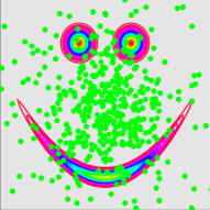
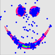
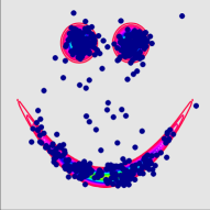
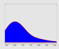
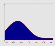
Figure 1: The target $f$ is a mixture of a banana shaped distribution and two Gaussians, The $\lambda_{k}$ are equal to $1$ for $k=0,\ldots,499$, to $0.1$ for $k=500,\ldots,999$ and to $0.05$ for $k=1000,\ldots,1499$. The $h_{k}$ are equal to $1$ all along the algorithm. The initial density $q_{0}$ is a standardized Student’s $t$-distribution. The particles indexed by $k=1,\ldots,500$ are on the left, $k=501,\ldots,1000$ are in the middle, $k=1001,\ldots,1500$ are on the right. At the bottom are density plots of the corresponding importance weights $W_{k}$.

3 Asymptotics of SAIS

3.1 Assumptions

The sequences $(\lambda_{k})_{k\geqslant 1}$, $(h_{k})_{k\geqslant 1}$ and $(\ell_{k})_{k\geqslant 1}$ are such that for any $k\geqslant 1$, $h_{k}$ is bounded and positive, $\lambda_{k}\in(0,1]$ is nonincreasing and $1\leqslant\ell_{k}\leqslant k$ is nondecreasing. For clarity reasons, the additional assumptions related to the sequences $(h_{k})_{k\geqslant 1}$, $(\lambda_{k})_{k\geqslant 1}$ and $(\ell_{k})_{k\geqslant 1}$ will be stated within the statements of each result. The results of the paper are expressed using the sequence

$$a_{n}=\sqrt{\frac{\log(n)}{nh_{n}^{d}}},\qquad n\geqslant 1,$$

and the following standard notation: for two nonnegative sequences $(u_{n})_{n\geqslant 1}$ and $(v_{n})_{n\geqslant 1}$, $u_{n}\ll v_{n}$ or $u_{n}=o(v_{n})$ means $u_{n}/v_{n}\to 0$ as $n\to\infty$; $u_{n}=O(v_{n})$ means that $u_{n}/v_{n}$ is bounded. The Euclidean norm is denoted by $\|\cdot\|$. The assumptions on $f_{U}$, $q_{0}$ and $K$ are given below. For clarity the assumptions are stated with respect to $f=f_{U}/\int f_{U}$ rather than $f_{U}$. They would have been the same using $f_{U}$.

1. $f$ is a probability density function on $\mathbb{R}^{d}$ two times continuously differentiable, with bounded second derivatives.

2. $q_{0}$ is a probability density function on $\mathbb{R}^{d}$. For any $\eta\in(0,1]$, there exists $c_{\eta}>0$ such that for all $x\in\mathbb{R}^{d}$

   $$f(x)^{\eta}\leqslant c_{\eta}q_{0}(x).$$

   In addition, there exist $C_{0}$ and $r_{0}$ positive numbers such that for all $x\in\mathbb{R}^{d}$

   $$q_{0}(x)\leqslant C_{0}(1+\|x\|)^{-r_{0}}.$$

3. $K:\mathbb{R}^{d}\to\mathbb{R}_{\geqslant 0}$ is a Lipschitz probability density function such that

   $$\int uK(u)\,\mathrm{d}u=0,\qquad\int\|u\|^{2}K(u)\,\mathrm{d}u<\infty.$$

   In addition, there exist $C_{K}$ and $r_{K}$ positive numbers such that for all $x\in\mathbb{R}^{d}$

   $$K(x)\leqslant C_{K}(1+\|x\|)^{-r_{K}}.$$

3.2 Preliminary results with general policy

Let us now present some results that are valid for a general policy

$$q_{k}=(1-\lambda_{k})f_{k}^{\circ}+\lambda_{k}q_{0},\qquad k\geqslant 1,$$ (3)

where $(f_{k}^{\circ})_{k\geqslant 1}$ is any sequence of densities adapted to the filtration $(\mathcal{F}_{k})_{k\geqslant 1}$. They will be useful in the analysis of standard SAIS (equation (1)) as well as in the study of the subsampling version (equation (2)). The proof of the following lemma is presented in Section 7.1.

Lemma 4 (initial bound).

Assume (H1), (H2), (H3) and work under a general policy (3). If $a_{n}^{2}\ll\lambda_{n}$, then we have,

$$\sup_{x\in\mathbb{R}^{d}}|f_{n}(x)-f(x)|=O\big{(}a_{n}\lambda_{n}^{-1/2}+h_{n}^{2}\big{)}\qquad\text{a.s.}$$

The next result, whose proof is given in Section 7.2, provides a sufficient rate of proximity between $f^{\circ}_{n}$ and $f$ allowing to improve the previous initial bound. That is, we shall assume that there exists $\varepsilon\in(0,1/2]$ such that

$$\sup_{x\in\mathbb{R}^{d}}|f^{\circ}_{n}(x)-f(x)|=O\big{(}\lambda_{n}^{1/2+\varepsilon}\big{)}\qquad\text{a.s.}$$ (4)

Lemma 5 (improved bound).

Assume (H1), (H2), (H3) and work under a general policy (3) that satisfies (4). If $a_{n}\ll\lambda_{n}$, we have

$$\sup_{x\in\mathbb{R}^{d}}|f_{n}(x)-f(x)|=O(a_{n}+h_{n}^{2}),\qquad\text{a.s.}$$

We terminate the section by two central limit theorems. Both require (4) to hold in order to obtain the appropriate asymptotic variance, i.e., the one associated to the policy $f$. The proof is in Section 7.3.

Lemma 6.

Assume (H1), (H2), (H3) and work under a general policy (3) that satisfies (4). If $a_{n}^{2}\ll\lambda_{n}\ll 1$, then for any function $g:\mathbb{R}^{d}\to\mathbb{R}$ such that $\int g^{2}q_{0}<\infty$, as $n\to\infty$,

$$\sqrt{n}\left(\sum_{k=1}^{n}W_{n,k}g(X_{k})-\int gf\right)\leadsto\mathcal{N}\big{(}0,V(f,g)\big{)},$$ (5)

where $V(f,g)$ is defined in Lemma 1.

3.3 Main results

Now we focus on the SAIS algorithms presented in Section 2. We start by considering standard SAIS. The subsampling version will be studied right after.

Assuming that for some $\epsilon>0$, $a_{n}+h_{n}^{4}\ll\lambda_{n}^{1+\varepsilon}$, we can apply Lemma 4 to obtain that (4) is valid with $f_{n}$ in place of $f_{n}^{\circ}$. This permits to apply Lemma 5 and leads to the following two results.

Theorem 7 (uniform convergence rate).

Assume (H1), (H2), (H3) and work under policy (1). If there exists $\epsilon>0$ such that $a_{n}+h_{n}^{4}\ll\lambda_{n}^{1+\epsilon}\ll 1$, we have with probability $1$

$$\sup_{x\in\mathbb{R}^{d}}|f_{n}(x)-f(x)|=O(a_{n}+h_{n}^{2}).$$

We now consider the weak convergence of the sequence $\sum_{k=1}^{n}W_{n,k}g(X_{k})$ for which we derive the asymptotic variance $V(f,g)$. The proof is a simple application of Lemma 4 and Lemma 6, equation (5).

Theorem 8 (asymptotic normality of integral estimates).

Assume (H1), (H2), (H3) and work under policy (1). If there exists $\epsilon>0$ such that $a_{n}+h_{n}^{4}\ll\lambda_{n}^{1+\epsilon}\ll 1$ and if $\int g^{2}q_{0}<\infty$, we have as $n\to\infty$, then (5) is valid.

Now let us consider SAIS with subsampling. The following result, whose proof is in Section 8, shows that subsampling is efficient as the convergence rate and the asymptotic variance are the same in Theorem 8.

Theorem 9 (asymptotic normality of integral estimates with subsampling).

Assume (H1), (H2), (H3) and work under the subbsampling policy (2). If there exists $\epsilon>0$ such that $a_{n}^{2}n/\ell_{n}+a_{n}+h_{n}^{4}\ll\lambda_{n}^{1+\epsilon}\ll 1$ and if $\int g^{2}q_{0}<\infty$, then (5) is valid.

4 From theory to practice

In this section, some comments dealing with the main results are given. Then we consider the practical tuning of the SAIS algorithms.

4.1 General comments on the main results

Related literature on kernel smoothing

Theorem 7 is related to uniform convergence results for kernel density estimates for independent sequences (Giné and Guillou, 2001, 2002), weak dependent sequences (Hansen, 2008), and Markov chains (Azaïs et al., 2018; Bertail and Portier, 2019). In these papers, the same rate of convergence, $\sqrt{\log(n)/(nh_{n}^{d})}$ (for the variance term), was obtained but under different assumptions on the dependence structure of the considered sequences.

Related literature on the asymptotics of AIS

The asymptotic regime that has been considered allows the distribution $q_{k}$ to change at each stage of the algorithm. This is similar to the regimes studied in Oh and Berger (1992), Delyon and Portier (2018), Feng et al. (2018) but different from the results presented in Chopin (2004), Douc et al. (2007a), Douc et al. (2007b) where the sequence $(q_{k})_{k=0,\ldots,n-1}$ is frozen after a certain given time (i.e., the number of updates is finite), or from Marin et al. (2019) where a variant of AIS is studied when the number of samples between each update is an increasing sequence going to $\infty$. Finally in Zhang (1996), the author works under another asymptotic regime in which the number of particles generated in the first stage has the same order as the total amount of particles.

Curse of dimensionality

Theorems 7 and 8 are of a different nature. Theorem 7 is dealing with functional estimation and, consequently, is subjected to the well-known curse of dimensionality (Stone, 1980). In contrast, the weak convergence result stated in Theorem 8, which is concerned with the estimation of a single parameter, $\int gf$, is not impacted by the value of $d$. This is because the estimation error between $f_{n}$ and $f$ intervenes at a second order in the decomposition used in the proof. This very last point motivated the subsampling version as it supports the use of rough but cheap strategies for the estimation of $f$.

Choice of the kernel

The kernel $K$ being non-negative (this is needed to ensure easy random generation according to $q_{n}$), it cannot have more than one vanishing moment. This bounds the exploitable smoothness of $f$ to two derivatives and explains why the rate of decrease of the bias term is ${h_{n}^{2}}$.

Asymptotic normality of the kernel estimate

Concerning the kernel estimate $f_{n}$, only uniform convergence results have been presented so far but the choice of the policy (1) has been motivated initially by a weak convergence result (see Lemma 2 and 3). A question that remains is to know whether the optimal variance given in Lemma 3, i.e., $f(x)\int K^{2}$ is achieved when the policy (1) is put to work. The answer is positive as stated in Theorem 8 given in Appendix A.

The compact case

When $f$ is compactly supported and bounded away from $0$, the study of the algorithm is simpler and similar results are valid under weaker conditions on $\lambda_{n}$ and $h_{n}$. This is presented in Appendix B.

4.2 Practical details

Choice of $(\lambda_{n},h_{n})$ for standard SAIS

If $h_{n}\propto n^{-\kappa}$ for some $\kappa<1$, then, balancing the variance term $a_{n}$ (up to a log) and the bias term ${h_{n}^{2}}$ in Theorem 7 leads to

$$h_{n}\propto n^{-1/(4+d)}.$$

The corresponding rate, $n^{-2/(4+d)}$ (up to a log), is the usual optimal rate in non parametric estimation when the function is at least $2$-times continuously differentiable and the kernel has order $2$ (Stone, 1980).

In practice, a slow decrease of $\lambda_{n}$ would favor an exhaustive visit of the space during what could be called the burn-in phase of the algorithm. Such a tuning of $\lambda_{n}$ might be appropriate when facing a difficult problem e.g., several modes or large variance of $f$. In contrast, a rapid decrease of $\lambda_{n}$ could be risky because the algorithm is likely to miss some important parts of the distribution. In Theorem 8, allowing $\lambda_{n}$ to go to $0$ only influences the asymptotic variance but the convergence rate remains the same. For instance, if $(\lambda_{k})_{k\geqslant 1}$ was converging to a constant $\lambda_{0}>0$, one would get $\sigma_{q}^{2}(x)\int K^{2}$, with $q=(1-\lambda_{0})f+\lambda_{0}q_{0}$, as asymptotic variance in Theorem 8 which would be fine in many cases as soon as $\lambda_{0}$ is small enough.

As expressed in Theorem 8, the only restriction we have on $\lambda_{n}$ is that it goes to $0$ not too quickly, i.e., $a_{n}+h_{n}^{4}\ll\lambda_{n}^{1+\epsilon}\ll 1$, for some $\epsilon>0$. Under the optimal bandwidth $h_{n}\propto n^{-1/(4+d)}$, an appropriate choice is

$$\lambda_{n}\propto n^{-1/(4+d)}.$$

Choice of $(\lambda_{n},h_{n},\ell_{n})$ for SAIS with subsampling

We discuss the subsampling version with $\ell_{n}=n^{\delta}$ (up to some rounding), where $\delta\in(0,1/2]$ encodes for the degree of subsampling. From Theorem 9, it is reasonable to balance between variance and bias, $a_{n}\sqrt{n/\ell_{n}}$ and $h_{n}^{2}$, to choose the bandwidth

$$h_{n}\propto\ell_{n}^{-1/(4+d)}.$$

Reasonably, the size of the bandwidth increases with the degree of subsampling. When $\delta\leqslant 1/2$, $a_{n}\propto n^{-(4+d(1-\delta))/(8+2d)}$ (up to a log) is negligible before $a_{n}\sqrt{n/\ell_{n}}\propto n^{-4\delta/(4+d)}$. Following Theorem 9, one can set

$$\lambda_{n}\propto\ell_{n}^{-2/(4+d)}.$$

Note that when $\delta=1/2$, we recover the same value as the one recommended for standard SAIS.

Updating $q_{0}$

A variant of the proposed approach is to use $q_{0}(\cdot-\mu_{k})$ with $\mu_{k}=\sum_{i=1}^{k}W_{k,i}X_{i}$ instead of $q_{0}$ in the policy (1). Such a policy should increase efficiency while staying in an heavy-tailed family of densities. This can be handled by a slight modification of our proofs. Because the sampler $q_{0}(\cdot-\mu_{k})$ now depends on $\mathcal{F}_{k}$, the condition needed, (H2), must be satisfied uniformly over $k$. This is certainly the case whenever $\mu_{k}$ is restricted to a compact set of $\mathbb{R}^{d}$.

Mini-batching

This is a common extra ingredient of AIS schemes. It consists in grouping the particles into “mini-batches” in which the particles have the same distribution. In other words, the policy $q_{k}$ is frozen over these mini-batches and the update of $q_{k}$ is conducted only when $k$ is entering a new mini-batch. This will save the time needed to update and allow to run in parallel the generation of the random variables according to $q_{k}$. For clarity reasons, the theoretical study to SAIS has been restricted to the case when each mini-batch is made of one sample point. The extension to mini-batches of size $m\geqslant 1$ with $mT=n$ can be carried out easily. Suppose that $(h_{k})_{k\geqslant 1}$ and $(\lambda_{k})_{k\geqslant 1}$ are just as in Lemma 4. Define the sequence $(\widetilde{q}_{t})_{t\geqslant 1}$ such that $\widetilde{q}_{t}=(1-\widetilde{\lambda}_{t})\widetilde{f}_{t}+\widetilde{\lambda}_{t}q_{0}$ where for each $t=1,\ldots,T$, $\widetilde{\lambda}_{t}=\lambda_{mt}$, $\widetilde{h}_{t}=h_{mt}$ and $\widetilde{f}_{t}=f_{mt}$. The mini-batch algorithm corresponds to the standard SAIS algorithm using $(q_{k})_{k\geqslant 1}$ given by

$$\widetilde{q}_{0},\ldots,\widetilde{q}_{0},\widetilde{q}_{1},\ldots,\widetilde{q}_{1},\ldots$$

Hence we can apply Lemma 4. With the obtained convergence rate, we can proceed similarly as before: apply Lemma 5 and 6, just as it has been done for proving Theorem 7 and 8.

5 Simulation study

The aim of the section is to illustrate the practical behavior of the SAIS algorithms. For the sake of reproducibility, we start by describing precisely the algorithms at use. Then two basic examples will be considered.

5.1 Algorithms

Here we bring together the pieces of information gathered in Section 4 to write down our ultimate SAIS algorithms (with and without subsampling). These very algorithms will be at use in the simulation study.

The allocation, $n\in\mathbb{N}^{*}$, is made of $T\in\mathbb{N}^{*}$ mini-batches containing $m_{0}=n/T\in\mathbb{N}^{*}$ particles. The set of particles indexes of any stage $t=1,\ldots,T$ is

$$B_{t}=\{1+(t-1)m,\ldots,tm\}.$$

Let $(h_{t})_{t=1,\ldots,T-1}$ be the sequence of bandwidths and $(\lambda_{t})_{t=1,\ldots,T-1}$ be the sequence of mixture weights. For any $t=1,\ldots,T$, define the discrete distribution associated to the weighted particles as

$$\mathbb{P}_{t}\propto\sum_{k=1}^{mt}W_{k}\delta_{X_{k}}.$$

The corresponding mean value is denoted $\mu_{t}$ and the associated kernel density estimate is given by

$$f_{t}(x)=\int K_{h_{t}}(x-y)\mathbb{P}_{t}(dy),\qquad x\in\mathbb{R}^{d}.$$

The policy at use in the mini-batch version is given by, for $t\geqslant 1$,

$$q_{t}(x)=(1-\lambda_{t})f_{t}(x)+\lambda_{t}q_{0}(x-\mu_{t}),\qquad x\in\mathbb{R}^{d}.$$ (6)

The algorithm includes a burn-in phase which corresponds to the first $T_{0}$ stages and, roughly speaking, aims at giving a tour in the target’s domain. During this early phase, the number of points is very small and the importance weights $W_{k}$ might have a large variance. To avoid the (uncommon) situation where a few weights carry all the mass of $\mathbb{P}_{t}$, we use regularized weights $W_{k}^{\eta}$, with $\eta\in(0,1)$, instead of $W_{k}$. This simple operation will uniformize the weights. The algorithm writes as follows.

SAIS with mini-batching
Inputs: Allocation $n$, number of stages $T$, bandwidths $(h_{t})_{t=1,\ldots,T-1}$, mixture weights $(\lambda_{t})_{t=1,\ldots,T-1}$, density $q_{0}$, initial mean $\mu_{\text{start}}$, burn-in parameters $(T_{0},\eta)$.  Initialize $\mu_{0}=\mu_{\text{start}}$. For $t=0,1,\ldots,T-1$:

• generate $(X_{k})_{k\in B_{t+1}}$ from $q_{t}$ in (6); compute $W_{k}=f_{U}(X_{k})/q_{t}(X_{k})$;

• if $t\leqslant T_{0}$, set $W_{k}=W_{k}^{\eta}$ for all $k\in B_{t+1}$.

 

In SAIS with subsampling, the policy is given by, for $t\geqslant 1$,

$$q_{t}(x)=(1-\lambda_{t})f_{t}^{*}(x)+\lambda_{t}q_{0}(x-\mu_{t}),\qquad x\in\mathbb{R}^{d},$$ (7)

where, in contrast with the standard SAIS, a bootstrap step will be needed at each stage to provide $f_{t}^{*}$, a bootstrap kernel estimate of $f$. The algorithm is written below.

SAIS with mini-batching and subsampling
Inputs: Allocation $n$, number of stages $T$, subsampling size $(\ell_{t})_{t=1,\ldots,T-1}$, bandwidths $(h_{t})_{t=1,\ldots,T-1}$, mixture weights $(\lambda_{t})_{t=1,\ldots,T-1}$, density $q_{0}$, initial mean $\mu_{\text{start}}$, burn-in parameters $(T_{0},\eta)$.  Initialize $\mu_{0}=\mu_{\text{start}}$. For $t=0,1,\ldots,T-1$:

• if $t\geqslant 1$, generate $(X_{k}^{*})_{k=1,\ldots,\ell_{t}}$ from $\mathbb{P}_{t}$; set $\mathbb{P}_{t}^{*}\propto\sum_{k=1}^{\ell_{t}}\delta_{X_{k}^{*}}$ and

  $$f_{t}^{*}(x)=\int K_{h_{t}}(x-y)\mathbb{P}_{t}^{*}(dy);$$

• generate $(X_{k})_{k\in B_{t+1}}$ from $q_{t}$ in (7); compute $W_{k}=f_{U}(X_{k})/q_{t}(X_{k})$;

• if $t\leqslant T_{0}$, set $W_{k}=W_{k}^{\eta}$ for all $k\in B_{t+1}$.

 

5.2 Methods in competition

In the simulation study, each method will be compared with an overall allocation equal to $n=200000$.

Standard SAIS

There is $T=200$ stages each generating $m=1000$ particles. For the burn-in phase, we take $T_{0}=20$ and $\eta=3/4$. Define $n_{0}=10000$. When no subsampling is performed, in agreement with Section 4, the values of $(h_{t},\lambda_{t})$ are given by

$$h_{t}=(0.4/\sqrt{d})(1+mt/n_{0})^{-1/(4+d)}$$

$$\lambda_{t}=0.25(1+mt/n_{0})^{-1/(4+d)}$$

for all $t=1,\ldots,T-1$ except for $\lambda_{t}$ during the burn-in phase where we simply set $\lambda_{t}=1$, $t=1,\ldots,9$ and $\lambda_{t}=.5$, $t=10,\ldots,19$. In the definition of the bandwidth, the factor $.4/\sqrt{d}$ corresponds to the standard error estimate in the Silverman’s rule of thumb Silverman (2018). Along the section this method is denoted SAIS.

Subsampling SAIS

Following Section 4 recommendation, at each iteration $t=1,\ldots,T-1$, the subsampling is carried out with $\ell_{t}=10\lfloor{(n_{0}+mt)^{\delta}}\rfloor$, where $\delta\in(0,1/2]$. Two versions of subsampling SAIS will be considered: SAIS*2 is when $\delta=1/2$ and SAIS*4 is when $\delta=1/4$. The values of $(h_{t},\lambda_{t})$ are given by

$$h_{t}=(0.4/\sqrt{d})(1+\ell_{t}/n_{0})^{-1/(4+d)}$$

$$\lambda_{t}=0.25(1+\ell_{t}/n_{0})^{-2/(4+d)}$$

for all $t=1,\ldots,T-1$ except during the burn-in phase, where $\lambda_{t}$ is tuned as before.

In both SAIS, $q_{0}$ is the student distribution with covariance matrix $(5/d)I_{d}$. The initial mean value $\mu_{\text{start}}$ will change depending on the considered example.

Metropolis-Hastings

Denote by $\phi_{\Sigma}$ the Gaussian density with mean $0$ and covariance matrix $\Sigma$. A natural competitor is the Metropolis-Hastings algorithm for which two proposals are considered. The random walk version is when the proposal is $\phi_{\Sigma}$ where $\Sigma=(0.4/d)I_{d}$. The adaptive Metropolis-Hastings, as introduced in Haario et al. (2001), denoted AMH, is when the proposal is $\phi_{\Sigma_{n}}$ with $\Sigma_{n}$ the estimated covariance matrix based on the past iterations of the chain. The adaptive proposal is put to work from iteration $1e4$. Before that, MH is used. For both Metropolis-Hastings algorithms, the starting point is $\mu_{\text{start}}$. Because, AMH produces better results than the standard version, we only provide the results of AMH.

Wang-Landau

Another natural competitor, which was initially designed to explore target densities with several modes, is the Wang-Landau algorithm (Wang and Landau, 2001), whose convergence properties are studied in Fort et al. (2015). The random walk version, denoted by WL, is when the proposal is $\phi_{\Sigma}$ with $\Sigma=(0.4/d)I_{d}$. The starting point is $\mu_{\text{start}}$. The adaptive version, which consists of a Robbins-Monro type of adaptation as documented in Bornn et al. (2013), has been tried without improving the results compared to the non-adaptive case. The PAWL package was used to run the Wang-Landau algorithm (without parallel chains and using an initial chain to tune optimally the bins which are parameters of the algorithm).

5.3 Results

5.3.1 Multimodal density

We revisit the classical example introduced in Cappé et al. (2008) in which the target density is a mixture of two Gaussian distributions. Let

$$f(x)=.5\phi_{\Sigma}(x-\mu)+.5\phi_{\Sigma}(x+\mu),\qquad x\in\mathbb{R}^{d},$$

with $\mu=(1,\ldots,1)^{T}/(2\sqrt{d})$ and $\Sigma=(0.4/d)I_{d}$. Note that the Euclidean distance between the two mixture centers is independent of the dimension as it equals $1$. The objective here is to recover both components of the mixture and this is clearly getting more difficult in large dimensions.

To measure the accuracy of the algorithms, we compute the squared Euclidean distance between the estimated mean and the true mean. For each method, we take $\mu_{\text{start}}=(1,-1,0,\ldots,0)^{T}/\sqrt{d}$ as starting point. Such a choice for the initial sampler is to prevent the algorithms to take advantage from a very good start as is the case when $\mu_{\text{start}}$ is $0$. We consider different values for the dimension $d$, namely $\{2,4,8,12\}$, and all the algorithms are compared using a budget going from $5.10^{4}$ to $2.10^{5}$ evaluations of $f$.

The results are presented in Figure 2 (except for the case $d=2$ which was similar to $d=4$). As expected, AMH gives poor results compared to the ones of SAIS and WL. This is because AMH can hardly leave a mode. Among the two other methods, after $2.10^{5}$ requests to $f$, the three SAIS methods give similar results. Compared to WL, the squared error of SAIS is reduced by at least a factor $10$ in every dimension and even more than that in dimension $12$.

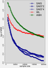
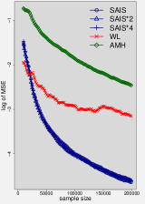
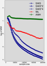
Figure 2: (multimodal density) From left-to-right $d=4,8,12$. Considered methods are described in the main text. Plotted is the median (based on $50$ independent replicates for each method) of the logarithm of the MSE with respect to the number of requests to the integrand.

5.3.2 Cold start

To conclude the simulation study, we illustrate the performance of SAIS when the starting distribution is far away from the target. In this example, the target distribution is given by $f(x)=\phi_{\Sigma}(x-\mu)$ where $\mu=(5,\ldots,5)^{T}/\sqrt{d}$ and $\Sigma=(1/d)I_{d}$ whereas the initial distribution (for all the considered methods) has mean $\mu_{\text{start}}=0$ and covariance $(4/d)I_{d}$. The main goal for the methods in competition is to converge rapidly around $\mu$. The error is the same as before, the squared Euclidean distance between the true mean and the estimated mean. We consider different values for the dimension $d$, namely $\{2,4,8,12\}$, and all the algorithms are compared using a budget going from $5.10^{4}$ to $2.10^{5}$ evaluations of $f$.

The results are shown in Figure 3 (except for $d=2$ which was similar to $d=4$). In this case, we observe a performance reversal between AMH and WL occurring at $d=8$. After that dimension, WL gives better results than MH. The improvement of SAIS compared to AMH and WL is substantial: the squared error is reduced by a factor $100$, in average.

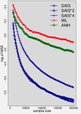
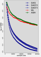
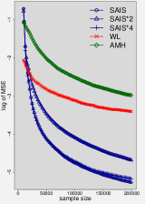
Figure 3: (cold start example) From left-to-right $d=4,8,12$. Considered methods are described in the main text. Plotted is the median (based on $50$ independent replicates for each method) of the logarithm of the MSE with respect to the number of requests to the integrand.

5.4 Computational efficiency

At each stage $t=1,\ldots,T-1$ of standard SAIS, the computing time needed to evaluate $q_{t}(X_{i})$, $i\in B_{t+1}$ is $tm^{2}$. Consequently, running the first $t$ iterations represents $c_{t}=m^{2}t(t-1)/2$ operations. Concerning SAIS with subsampling, the situation is different as already discussed in Section 2. For the first $t$ iterations, an estimate of the number of operations required is then $m\sum_{k=1}^{t}\ell_{k}$, neglecting a log factor (due to multinomial sampling as detailed in Section 2). For the standard and the subsampling variants, the graphs representing the accuracy versus the computing time are provided in Figure 4 in a logarithmic scale. We see a clear improvement given by the use of subsampling. For a similar error value, the overall computing time is almost $2$ times smaller in the logarithmic scale. This is a substantial gain as it means that in terms of computing time subsampling SAIS is approximately the square root of standard SAIS.

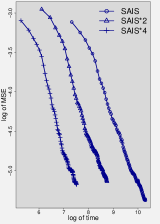
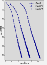
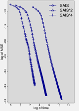
Figure 4: From left-to-right $d=4,8,12$. Considered methods are described in the main text. Plotted is the median (based on $50$ independent replicates for each method) of the logarithm of the MSE with respect to the number of requests to the integrand.

6 Mathematical proofs

All the claims of the theorems depend on $f_{U}(X_{i})$ only through $W_{n,i}$, $i=1,\ldots,n$, which is independent of any normalizing constant. As a consequence we can assume without loss of generality that $f_{U}=f$ in the proofs.

6.1 Proof of Lemma 2

We start with some preliminary remarks. Recall that for each $i\geqslant 1$ $W_{i}=f(X_{i})/q(X_{i})$, and that

$$\widetilde{f}_{n}=f*K_{h_{n}},$$

and define

$$A_{n}(x)=n^{-1}\Big{(}\sum_{i=1}^{n}W_{i}\Big{)}\left(f_{n}(x)-\widetilde{f}_{n}(x)\right),$$

$$K_{i}=K_{h_{n}}(x-X_{i}).$$

By assumption, $(X_{i})_{i\geqslant 1}$ is a sequence of independent random variables each having density $q$. Moreover, $\sigma_{q}^{2}$ is continuous and bounded on $\mathbb{R}^{d}$ and integrable. The assumption on $K$ ensures that $\int K^{2}<\infty$. In particular, we have

$$\mathbb{E}\left(\sum_{i=1}^{n}\{W_{i}-1\}\right)^{2}=n\mathbb{E}\{W_{1}-1\}^{2}\leqslant n\int\sigma_{q}^{2}.$$

Let $x\in\mathbb{R}^{d}$. From Slutsky Lemma, because $n^{-1}\left(\sum_{i=1}^{n}W_{i}\right)\to 1$ in probability, the proof will be complete as soon as we obtain that $(nh_{n}^{d})^{1/2}A_{n}(x)\leadsto\mathcal{N}(0,\sigma_{q}^{2}(x)\int K^{2})$. We have

$$\sqrt{nh^{d}}\,A_{n}(x) =\sqrt{h_{n}^{d}/n}\,\left(\sum_{i=1}^{n}W_{i}\right)\left(\sum_{i=1}^{n}W_{n,i}\big{(}K_{i}-\widetilde{f}_{n}(x)\big{)}\right)$$

$$=\sqrt{h_{n}^{d}/n}\,{\sum_{i=1}^{n}W_{i}\big{(}K_{i}-\widetilde{f}_{n}(x)\big{)}}$$

$$=\sqrt{h_{n}^{d}/n}\,\left(\sum_{i=1}^{n}\big{\{}W_{i}K_{i}-\widetilde{f}_{n}(x)\big{\}}-\widetilde{f}_{n}(x)\sum_{i=1}^{n}\{W_{i}-1\}\right),$$

Using that $\widetilde{f}_{n}(x)\leqslant\sup_{x\in\mathbb{R}^{d}}f(x)$, we obtain that

$$\sqrt{nh_{n}^{d}}\,A_{n}(x)=\sqrt{h_{n}^{d}/n}\,\sum_{i=1}^{n}\big{\{}W_{i}K_{i}-\widetilde{f}_{n}(x)\big{\}}+O_{P}(h_{n}^{d/2}).$$

Invoking Slutsky Lemma again, and using that $h_{n}\to 0$, it suffices to show that

$$\sqrt{h_{n}^{d}/n}\,\sum_{i=1}^{n}\big{\{}W_{i}K_{i}-\widetilde{f}_{n}(x)\big{\}}\leadsto\mathcal{N}\Big{(}0,\sigma_{q}^{2}(x)\int K^{2}\Big{)}.$$

Noting that $\sum_{i=1}^{n}\{W_{i}K_{i}-\widetilde{f}_{n}(x)\}=\sum_{i=1}^{n}\{W_{i}K_{i}-\mathbb{E}[W_{i}K_{i}]\}$, this convergence will be obtained by applying the Lindeberg central limit theorem (van der Vaart, 1998, Theorem 2.27). We have to check the convergence of covariances to $\sigma_{q}^{2}(x)\int K^{2}$ and the Lindeberg condition. Because the elements of the previous sum are independent and centered, the covariance convergence means that

$$h_{n}^{d}\big{(}\mathbb{E}[W_{1}^{2}K_{1}^{2}]-\mathbb{E}[W_{1}K_{1}]^{2}\big{)}\to\sigma_{q}^{2}(x)\int K^{2}.$$

Recall that for any integrable and continuous function $g$, we have $(g\ast K_{h})(x)\to g(x)$ as $h\to 0$, for all $x\in\mathbb{R}^{d}$ (see Section 8 of Folland (2013)). On the first hand, introducing the kernel $\widetilde{K}=K^{2}/\int K^{2}$, it holds that

$$h_{n}^{d}\mathbb{E}[W_{1}^{2}K_{1}^{2}] =h_{n}^{d}\int\frac{f(y)^{2}}{q(y)}K\big{(}(x-y)/h_{n}\big{)}^{2}/h_{n}^{2d}\mathrm{d}y$$

$$=\Big{(}\int K^{2}\Big{)}(\sigma_{q}^{2}*\widetilde{K}_{h_{n}})(x)\longrightarrow\sigma_{q}^{2}(x)\int K^{2}.$$

On the other hand, one has $\mathbb{E}[W_{1}K_{1}]^{2}=(f*K_{h})(x)^{2}\to f(x)^{2}$, which implies that the second term in the variance is $O(h_{n}^{d})$, negligible. We finally need to verify the Lindeberg condition, i.e., for any $\epsilon>0$

$$\lim_{n\to\infty}\frac{h_{n}^{d}}{n}\sum_{i=1}^{n}\mathbb{E}\left[W_{i}^{2}K_{i}^{2}1_{\{|W_{i}K_{i}|>\epsilon\sqrt{n/h_{n}^{d}}\}}\right]=0.$$

Because $W_{i}$ is bounded by $c$ and $K_{i}$ is bounded by $h_{n}^{-d}\sup_{x\in\mathbb{R}^{d}}K(x)$ we have that $\{|W_{i}K_{i}|>\epsilon\sqrt{n/h_{n}^{d}}\}\subset\{C>\epsilon\sqrt{nh_{n}^{d}}\}$ for some $C>0$. But because $nh_{n}^{d}\to+\infty$, the previous set is empty for $n>n(\epsilon)$, implying the above statement. ∎

6.2 Proof of Lemma 3

If $q$ does not dominate $f$ then $\int f^{2}/q=+\infty$. If it does, using the Cauchy-Schwarz inequality, we obtain $1=(\int f)^{2}=(\int(f/\sqrt{q})\sqrt{q})^{2}\leqslant\int f^{2}/q=C(q)$. From this we deduce that $q=f$ is an argmin. If now $q$ is such that $\int f^{2}/q=1$, then equality holds in the Cauchy-Schwarz inequality meaning that $f=\kappa q$ a.e. with $\kappa>0$. But $\kappa$ needs to be $1$ because $q$ and $f$ are densities. ∎

7 Proof of the preliminary results

Before entering the proofs of the preliminary results, let us introduce some notation related to the assumptions (H1), (H2) and (H3). As the function $f$, $K$ and $q_{0}$ are bounded, we denote by $U_{f}>0$, $U_{K}>0$ and $U_{q_{0}}>0$ their respective uniform bounds, i.e., for all $x\in\mathbb{R}^{d}$,

$$f(x)\leqslant U_{f},\qquad K(x)\leqslant U_{K},\qquad q_{0}(x)\leqslant U_{q_{0}}.$$

The Lipschitz constant of the function $K$ is denoted by $L_{K}$, that is, for all $(x,y)\in\mathbb{R}^{d}\times\mathbb{R}^{d}$,

$$|K(x)-K(y)|\leqslant L_{K}\|x-y\|.$$

7.1 Proof of Lemma 4

Define

$$Z_{n}(x)=\sum_{i=1}^{n}\big{\{}W_{i}K_{h_{n}}(x-X_{i})-\widetilde{f}_{n}\big{\}},$$

$$M_{n}=\sum_{i=1}^{n}\left\{W_{i}-1\right\}.$$

The proof will follow from the use of $3$ independent lemmas which are now stated and proved.

Lemma 10.

Assume (H1), (H2), (H3) and work under the general policy (3). If $a_{n}^{2}\ll\lambda_{n}$, then we have, for any $s>0$,

$$|M_{n}|=O(\lambda_{n}^{-1/2}\sqrt{n\log n})=o(n),\quad\text{a.s.}$$ (8)

$$\sup_{\|x\|\leqslant n^{s}}|Z_{n}(x)|=O(na_{n}\lambda_{n}^{-1/2}),\quad\text{a.s.}$$ (9)

Moreover, if for any $s>0$, with probability $1$,

$$\sup_{\|x\|\leqslant n^{s}}|f_{n}(y)-\widetilde{f}_{n}(y)|=O\big{(}a_{n}\lambda_{n}^{-1/2}\big{)}.$$ (10)

Proof.

Equation (10) will follow from the decomposition

$$f_{n}(x)-\widetilde{f}_{n}(x)=\frac{Z_{n}(x)-\widetilde{f}_{n}(x)M_{n}}{M_{n}+n}.$$ (11)

Using (8) and (9), combined with $\log(n)/(n\lambda_{n})\to 0$ (since $a_{n}^{2}\ll\lambda_{n}$), we obtain that, almost surely,

$$\sup_{\|x\|\leqslant n^{s}}\big{|}f_{n}(x)-\widetilde{f}_{n}(x)\big{|}=O\big{(}a_{n}\lambda_{n}^{-1/2}\big{)}+O\big{(}\lambda_{n}^{-1/2}\sqrt{\log(n)/n}\big{)}=O\big{(}a_{n}\lambda_{n}^{-1/2}\big{)}.$$

The proof of (8) follows from Theorem 17 with $Y_{i}=f(X_{i})/q_{i-1}(X_{i})-1$. Recall the definition of $c_{\eta}$ in (H2). In particular, $f(x)\leqslant c_{1}q_{0}(x)$ for all $x\in\mathbb{R}^{d}$. Note that, for any $i=1,\ldots,n$,

$$\sup_{x\in\mathbb{R}^{d}}\frac{f(x)}{q_{i-1}(x)}\leqslant c_{1}\lambda_{n}^{-1}.$$ (12)

Since $|Y_{i}|\leqslant{m}=\lambda_{n}^{-1}c_{1}+1$, and the quadratic variation is not larger than $v=n\lambda_{n}^{-1}c_{1}$, we get

$$\mathbb{P}\big{(}|M_{n}|\geqslant t\big{)}\leqslant 2\exp\left(-\frac{Ct^{2}\lambda_{n}}{n+t}\right),$$

for some constant $C>0$ depending on $f$ and $q_{0}$. We conclude by taking $t=\gamma\sqrt{n\log n/\lambda_{n}}$ for $\gamma$ large enough and use the Borel-Cantelli lemma.

We now consider (9). Let us apply Corollary 20 with $\varepsilon=h_{n}^{d+1}n^{-1}$, $\Omega_{1}=\Omega$, and

$$W_{i}=\frac{f(X_{i})}{q_{i-1}(X_{i})},\qquad\mu(dx)=f(x)dx,\qquad M(x)=c_{1}\lambda_{n}^{-1}.$$

It remains to choose $t$ and evaluate $m$, $\widetilde{v}$ and $\tau$. We have, with the notation of Corollary 20

$$m=U_{K}(1+c_{1}\lambda_{n}^{-1})h_{n}^{-d}\leqslant C\lambda_{n}^{-1}h_{n}^{-d}$$

$$v=nh_{n}^{-d}U_{K}\int M(u)K_{h_{n}}(x-u)\mu(du)\leqslant Cnh_{n}^{-d}\lambda_{n}^{-1}$$

$$\tau=2L_{K}\varepsilon nh_{n}^{-d-1}=2L_{K}$$

$$\widetilde{v}=\max(v,2m\tau)\leqslant Cnh_{n}^{-d}\lambda_{n}^{-1}$$

for some $C>0$. Taking $t=\gamma\sqrt{nh_{n}^{-d}\lambda_{n}^{-1}\log n}$ for $\gamma\geqslant 1$, the conclusion of Corollary 20 is

$$\mathbb{P}\Big{(}\sup_{\|x\|\leqslant n^{s}}|Z_{n}(x)|>t+\tau\Big{)}\leqslant 4\Big{(}1+\frac{2n^{s+1}}{h_{n}^{d+1}}\Big{)}^{d}\exp\left(-\frac{t^{2}}{8(\widetilde{v}+2mt/3)}\right).$$

The term in the exponential is smaller than

$$-\frac{\gamma^{2}n\log n}{8Cn(1+\gamma\sqrt{\log n/(nh_{n}^{d}\lambda_{n})})}.$$

Because $a_{n}^{2}=o(\lambda_{n})$, the denominator is dominated by $8Cn$ and we get, since $t\geqslant\tau$ (for $n$ large enough),

$$\mathbb{P}\Big{(}\sup_{\|x\|\leqslant n^{s}}|Z_{n}(x)|>2\gamma\sqrt{nh_{n}^{-d}\lambda_{n}^{-1}\log n}\Big{)}\leqslant 4\Big{(}1+\frac{2n^{s+1}}{h_{n}^{d+1}}\Big{)}^{d}\exp\left(-C_{1}\gamma^{2}\log n\right)$$

for some $C_{1}>0$. With $\gamma$ large enough, we obtain

$$\sum_{n\geqslant 1}\mathbb{P}\left(\sup_{\|x\|\leqslant n^{s}}|Z_{n}(x)|>2\gamma\sqrt{n\log(n)/h_{n}^{d}\lambda_{n}}\right)<+\infty,$$

which by the Borel-Cantelli lemma implies (9). ∎

Lemma 11.

Under (H1) and (H3), it holds that $\sup_{x\in\mathbb{R}^{d}}\big{|}\widetilde{f}_{n}(x)-f(x)\big{|}=O(h_{n}^{2})$.

Proof.

Write

$$\big{|}\widetilde{f}_{n}(x)-f(x)\big{|} =\Big{|}\int\big{(}f(x+h_{n}y)-f(x)\big{)}K(y)dy\Big{|}$$

$$=\Big{|}\int\big{(}f(x+h_{n}y)-f(x)-h_{n}\langle y,\nabla f(x)\rangle\big{)}K(y)dy\Big{|}$$

$$\leqslant\frac{h_{n}^{2}}{2}\sup_{x\in\mathbb{R}^{d}}|\nabla^{2}f(x)|\Big{(}\int\|y\|^{2}K(y)dy\Big{)}.\qed$$

Lemma 12.

Assume (H1), (H2), (H3) and work under the general policy (3). If $a_{n}^{2}\ll\lambda_{n}$, then there exists $s_{0}>0$ large enough such that

$$\sup_{\|x\|>n^{s_{0}}}f_{n}(x)=o(a_{n}),\quad a.s.,$$ (13)

$$\sup_{\|x\|>n^{s_{0}}}f(x)=o(a_{n}).$$ (14)

Proof.

Let us start with (13). Because $a_{n}^{2}\ll\lambda_{n}$, one has $nh_{n}^{d}\to\infty$ and $\log(n)/n\ll\lambda_{n}$. We write

$$f_{n}(x)=\sum_{i=1}^{n}W_{n,i}K_{h_{n}}(x-X_{i})(\mathds{1}_{\{\|X_{i}\|\leqslant n^{s_{0}}/2\}}+\mathds{1}_{\{\|X_{i}\|>n^{s_{0}}/2\}})$$

and treat both term separately. Using that $\sum_{i=1}^{n}W_{n,i}=1$ and (H3), we find for any $\|x\|>n^{s_{0}}$,

$$\sum_{i=1}^{n}W_{n,i}K_{h_{n}}(x-X_{i})\mathds{1}_{\{\|X_{i}\|\leqslant n^{s_{0}}/2\}} \leqslant\sup_{\|y\|\leqslant n^{s_{0}}/2}K_{h_{n}}(x-y)$$

$$=C_{K}h_{n}^{-d}\sup_{\|y\|\leqslant n^{s_{0}}/2}(1+\|x-y\|/h_{n})^{-r_{K}}$$

$$=C_{K}h_{n}^{-d}(1+n^{s_{0}}/(2h_{n}))^{-r_{K}}.$$

This bound being $O(h_{n}^{-d+r_{K}}n^{-s_{0}r_{K}})$ and $nh_{n}^{d}\to\infty$, one might choose $s_{0}$ to make it $O(n^{-1/2})=o(a_{n})$. For the other term, start with the bound

$$\sum_{i=1}^{n} W_{n,i}K_{h_{n}}(x-X_{i})\mathds{1}_{\{\|X_{i}\|>n^{s_{0}}/2\}}\leqslant U_{K}h_{n}^{-d}\sum_{i=1}^{n}W_{n,i}\mathds{1}_{\{\|X_{i}\|>n^{s_{0}}/2\}}.$$

Because $\log(n)/n\ll\lambda_{n}$, we can use (8) to obtain, with probability $1$,

$$\sum_{i=1}^{n}W_{n,i}\mathds{1}_{\{\|X_{i}\|>n^{s_{0}}/2\}} =\frac{1}{M_{n}+n}\sum_{i=1}^{n}\frac{f(X_{i})}{q_{i-1}(X_{i})}\mathds{1}_{\{\|X_{i}\|>n^{s_{0}}/2\}}$$

$$\leqslant O(1)(n\lambda_{n})^{-1}\sum_{i=1}^{n}\frac{f(X_{i})}{q_{0}(X_{i})}\mathds{1}_{\{\|X_{i}\|>n^{s_{0}}/2\}}.$$

Notice that assumption (H2), with $\varepsilon$ small, implies that for any $p\geqslant 1$, there exists $C_{p}>0$ such that

$$f(x)/q_{0}(x)=C_{p}(1+\|x\|)^{-p},\qquad\|x\|\to+\infty.$$ (15)

It follows that

$$\sum_{i=1}^{n}\frac{f(X_{i})}{q_{0}(X_{i})}\mathds{1}_{\{\|X_{i}\|>n^{s_{0}}/2\}} \leqslant C_{p}\sum_{i=1}^{n}(1+\|X_{i}\|)^{-p}\mathds{1}_{\{\|X_{i}\|>n^{s_{0}}/2\}}$$

$$\leqslant C_{p}n(1+n^{s_{0}}/2)^{-p}.$$

Since $\lambda_{n}^{-1}h_{n}^{-d}\ll a_{n}^{-2}h_{n}^{-d}\ll n$, we obtain with probability $1$,

$$\sum_{i=1}^{n}W_{n,i}K_{h_{n}}(x-X_{i})\mathds{1}_{\{\|X_{i}\|>n^{s_{0}}/2\}}=O(\lambda_{n}^{-1}h_{n}^{-d}n^{-ps_{0}})=o(n^{1-ps_{0}}).$$

Choose $p$ large enough to obtain that the previous bound is $o(n^{-1/2})=o(a_{n})$. Equation (14) is clearly a consequence of (15) ∎

End of the proof of Lemma 4

Choose $s_{0}$ large enough so that the conclusion of Lemma 12 is valid. We have

$$|f_{n}(x)-f(x)| \leqslant\sup_{\|x\|\leqslant n^{s_{0}}}|f_{n}(x)-f(x)|+\sup_{\|x\|>n^{s_{0}}}f_{n}(x)+f(x)$$

$$\leqslant\sup_{\|x\|\leqslant n^{s_{0}}}|f_{n}(x)-\widetilde{f}_{n}(x)|+\sup_{x\in\mathbb{R}^{d}}|\widetilde{f}_{n}(x)-f(x)|$$

$$\qquad\qquad\qquad\qquad\qquad\qquad\qquad+\sup_{\|x\|>n^{s_{0}}}f_{n}(x)+f(x)$$ (16)

Lemma 11 implies that the middle term is $O(h_{n}^{2})$. Lemma 12 implies that the right-hand side term is $o(a_{n})$ almost surely. Lemma 10 implies that the left-hand side term is $O\big{(}a_{n}\lambda_{n}^{-1/2}\big{)}$.∎

7.2 Proof of Lemma 5

The proof is similar to the proof of Lemma 4. The only difference is that, instead of using the bound (10), we shall use an improved bound on $\sup_{\|x\|\leqslant n^{s}}|f_{n}(x)-\widetilde{f}_{n}|$ which will follow from the additional assumption (4). This bound will be given in Lemma 14 but before we need to obtain the following technical lemma which will be used several times in the sequel.

Lemma 13.

Assume (H1), (H2), (H3) and work under the general policy (3). If $a_{n}^{2}\ll\lambda_{n}$, then we have for any $\varepsilon\in(0,1/2)$

$$\sup_{i\geqslant 0}\sup_{x\in\mathbb{R}^{d}}\lambda_{i}^{-\varepsilon}f(x)\Big{|}\frac{f(x)}{q_{i}(x)}-1\Big{|}=O(1),\quad a.s.$$ (17)

$$\sup_{i\geqslant 0}\sup_{x\in\mathbb{R}^{d}}\frac{f^{2}(x)}{q_{i}(x)q_{0}(x)}<+\infty,\quad a.s.$$ (18)

Proof.

Set

$$d_{i}=\sup_{x\in\mathbb{R}^{d}}|q_{i}(x)-f(x)|.$$

Since $f$ and $q_{0}$ are bounded, (4) implies clearly that $d_{i}=O(\lambda_{i}^{1/2+\varepsilon})$ a.s. If $f(x)\leqslant 2d_{i}$, (H2) implies, for $i$ large enough,

$$f(x)\leqslant f(x)^{1-\varepsilon}c_{\epsilon}q_{0}(x)\leqslant(2d_{i})^{1-\varepsilon}c_{\epsilon}q_{i}(x)/\lambda_{i}\leqslant C_{1}\lambda_{i}^{-\frac{1}{2}}q_{i}(x),$$

for some $C_{1}>0$ (because $\varepsilon\leqslant 1/2$). If $f(x)>2d_{i}$, we have $q_{i}(x)>d_{i}$ but $f(x)-q_{i}(x)\leqslant d_{i}$ implying that $f(x)\leqslant 2q_{i}(x)$, thus $f(x)\leqslant 2\lambda_{i}^{-\frac{1}{2}}q_{i}(x)$. In any case $f(x)\leqslant(C_{1}+2)\lambda_{i}^{-\frac{1}{2}}q_{i}(x)$ and this leads to the bound

$$f(x)|f(x)-q_{i}(x)|\leqslant C_{1}^{\prime}\lambda_{i}^{-\frac{1}{2}}q_{i}(x)\lambda_{i}^{\frac{1}{2}+\varepsilon}$$

which implies (17). For (18), notice that because the $q_{i}$ are uniformly bounded (by $U_{f}+\sup_{i}d_{i}$), one has that $q_{0}^{1/2+\epsilon}q_{i}^{1/2-\epsilon}$ is uniformly bounded by some $C_{2}>0$. Then, since $d_{i}=O(\lambda_{i}^{1/2+\varepsilon})$,

$$f(x)\leqslant q_{i}(x)+C_{3}\lambda_{i}^{\frac{1}{2}+\varepsilon}\leqslant q_{i}(x)+C_{3}\Big{(}\frac{q_{i}(x)}{q_{0}(x)}\Big{)}^{\frac{1}{2}+\varepsilon}\leqslant(C_{2}+C_{3})\Big{(}\frac{q_{i}(x)}{q_{0}(x)}\Big{)}^{\frac{1}{2}+\varepsilon},$$

for some $C_{3}>0$. Now

$$f(x)^{2}=f(x)^{(\frac{1}{2}+\varepsilon)^{-1}}f(x)^{\frac{4\varepsilon}{1+2\varepsilon}}\leqslant C_{4}\frac{q_{i}(x)}{q_{0}(x)}q_{0}(x)^{2},$$

where $C_{4}$ is given by using (H2). This is (18). ∎

Lemma 14.

Assume (H1), (H2), (H3) and work under the general policy (3). If $a_{n}=O(\lambda_{n})$, we have for any $s>0$, with probability $1$,

$$\sup_{\|x\|\leqslant n^{s}}\,|Z_{n}(x)|=O\left(\sqrt{\frac{n\log(n)}{h_{n}^{d}}}\right)$$ (19)

$$|M_{n}|=O\big{(}\sqrt{n\log n}\big{)}.$$ (20)

Moreover, for any $s>0$, with probability $1$,

$$\sup_{\|x\|\leqslant n^{s}}|f_{n}(y)-\widetilde{f}_{n}(y)|=O(a_{n}).$$ (21)

Proof.

Equation (11), namely $f_{n}(y)-\widetilde{f}_{n}(y)=(Z_{n}(y)-\widetilde{f}_{n}(y)M_{n})/(M_{n}+n)$, implies that (21) follows from (19) and (20).

In order to prove (19), we will use Corollary 20 with

$$\Omega_{1}=\Omega_{U}=\left\{\omega:\sup_{i\geqslant 0}\sup_{x\in\mathbb{R}^{d}}\frac{f^{2}(x)}{q_{i}(x)q_{0}(x)}\leqslant U\right\}$$

where $U$ is a parameter, and

$$W_{i}=\frac{f(X_{i})}{q_{i-1}(X_{i})},\quad\mu(dy)=f(y)dy,\quad M(x)=\left(U\frac{q_{0}(x)}{f(x)}\right)\wedge\left(c_{1}\lambda_{n}^{-1}\right).$$

It remains to choose $t$ and $\varepsilon$ and to evaluate $m$, $\widetilde{v}$ and $\tau$. As in the proof of Lemma 10, we take $\varepsilon=h_{n}^{d+1}n^{-1}$, and

$$m=U_{K}(1+U_{w})h_{n}^{-d}\leqslant U_{K}(1+c_{1}\lambda_{n}^{-1})h_{n}^{-d}$$

$$v=U_{K}nh_{n}^{-d}\int M(u)K_{h_{n}}(x-u)f(u)du\leqslant U_{K}nh_{n}^{-d}U_{q_{0}}U$$

$$\tau=2L_{K}\varepsilon_{n}nh_{n}^{-d-1}=2L_{K}$$

$$\widetilde{v}=\max(v,2m\tau).$$

The conclusion of Corollary 20 is that, for all $t\geqslant 0$,

$$\mathbb{P}\Big{(}\sup_{\|x\|\leqslant n^{s}}|Z_{n}(x)|>t+\tau,\,\Omega_{U}\Big{)}\leqslant 4(1+2n^{s}/\varepsilon)^{d}\exp\left(-\frac{t^{2}}{8(\widetilde{v}+2mt/3)}\right).$$

We take $t=\gamma\sqrt{n\log(n)h_{n}^{-d}}$, and notice that $t\geqslant\tau$ for $n$ large enough. Using that $\lambda_{n}^{-1}=O(a_{n}^{-1})$, we find that $mt\leqslant C\gamma\lambda_{n}^{-1}h_{n}^{-d}\sqrt{n\log(n)h_{n}^{-d}}\leqslant C\gamma nh_{n}^{-d}$ and also $\widetilde{v}\leqslant Cnh_{n}^{-d}$, when $n$ is large enough, for some $C>0$. Taking $\gamma$ larger than $3/2$, we find

$$\mathbb{P}\Big{(}\sup_{\|x\|\leqslant n^{s}}|Z_{n}(x)|>2t,\,\Omega_{U}\Big{)} \leqslant 4\Big{(}1+\frac{2n^{s+1}}{h_{n}^{d+1}}\Big{)}^{d}\exp\left(-\frac{3t^{2}}{32C\gamma nh_{n}^{-d}}\right)$$

$$\leqslant 4\Big{(}1+\frac{2n^{s+1}}{h_{n}^{d+1}}\Big{)}^{d}\exp\left(-3\gamma\log(n)/(32C)\right).$$

For $\gamma$ large enough, the Borel-Cantelli lemma applies and one has for any $U>0$ that

$$\mathbb{P}\left(\limsup_{n\to\infty}\sup_{\|x\|\leqslant n^{s}}\frac{|Z_{n}(x)|}{\sqrt{n\log(n)h_{n}^{-d}}}>\gamma,\,\Omega_{U}\right)=0$$

which implies the result since, by Lemma 13, $\mathbb{P}(\Omega_{U})\to 1$ as $U\to+\infty$.

The proof of (20) will use Theorem 17. The bounds on the quadratic variation and the increments of $M_{n}$ are derived in a very similar way as before. By (12) and $\lambda_{n}^{-1}=O(a_{n}^{-1})$, we have

$$\max_{i=1,\ldots,n}\sup_{y\in\mathbb{R}^{d}}\left|\frac{f(y)}{q_{i-1}(y)}-1\right|\leqslant c_{1}\lambda_{n}^{-1}+1\leqslant C\Big{(}\frac{n}{\log n}\Big{)}^{1/2}=m$$

$$\sum_{i=1}^{n}\int\frac{f(y)^{2}}{q_{i-1}(y)}\,\mathrm{d}y\leqslant nU=v\quad\text{on $\Omega_{U}$}.$$

Theorem 17 implies that for any $t>0$

$$\mathbb{P}\left(|M_{n}|>t,\Omega_{U}\right) =\exp\Bigg{(}-\frac{t^{2}}{2(nU+(C/3)t\sqrt{n/\log n})}\Bigg{)}.$$

Choosing $t=\gamma\sqrt{n\log n}$ with $\gamma$ large leads to the summability of these probabilities and (20) holds on $\Omega_{U}$. Since $\mathbb{P}(\Omega_{U})\to 1$ as $U\to\infty$ (Lemma 13), we get (20). ∎

7.3 Proof of Lemma 6

We rely on the following central limit theorem for martingale arrays.

Theorem 15.

(Hall and Heyde, 1980, Corollary 3.1) Let $(w_{n,i})_{1\leqslant i\leqslant n,\,n\geqslant 1}$ be a triangular array of random variables such that

$$\mathbb{E}[w_{n,i}\mid\mathcal{F}_{i-1}]=0,\quad\text{for all }1\leqslant i\leqslant n,$$ (22)

$$\sum_{i=1}^{n}\mathbb{E}[w_{n,i}^{2}\mid\mathcal{F}_{i-1}]\to v^{*}\geqslant 0,\quad\text{in probability,}$$ (23)

$$\sum_{i=1}^{n}\mathbb{E}[w_{n,i}^{2}\mathrm{I}_{\{|w_{n,i}|>\varepsilon\}}\mid\mathcal{F}_{i-1}]\to 0,\quad\text{in probability,}$$ (24)

then, $\sum_{i=1}^{n}w_{n,i}\leadsto\mathcal{N}(0,v^{*})$, as $n\to\infty$.

Proof of equation (5)

Set

$$I_{n}(g)=n^{-1}\sum_{i=1}^{n}W_{i}g(X_{i})$$

Because $\log(n)/n\ll\lambda_{n}$, applying Lemma 10 gives that $I_{n}(1)$ converges in probability to $1$. Using the decomposition

$$\sum_{i=1}^{n}W_{n,i}g(X_{i})-I(g)=\frac{1}{I_{n}(1)}\left\{\Big{(}I_{n}(g)-I(g)\Big{)}-\big{(}I_{n}(1)-1\big{)}I(g)\right\},$$

with $I(g)=\int gf$, the problem reduces to the estimation of the limit of $n^{1/2}((I_{n}(g)-I(g)),(I_{n}(1)-1))$. Verifying the conditions of Theorem 15 with $v_{*}=V(f,g)$ and

$$w_{n,i}=\frac{1}{\sqrt{n}}\Big{(}\frac{g(X_{i})f(X_{i})}{q_{i-1}(X_{i})}-I(g)\Big{)},$$

will prove the convergence of $n^{1/2}(I_{n}(g)-I(g))$ to the limit $\mathcal{N}(0,V(f,g))$. This will imply that $n^{1/2}(I_{n}(1)-1)$ converges to zero in probability since $V(f,1)=0$, and the result will follow by virtue of Slutsky’s Lemma.

Equation (22) is satisfied. We now show (23) with $v_{*}=V(f,g)=\int g^{2}f-I(g)^{2}$, or equivalently that

$$n^{-1}\sum_{i=1}^{n}\int\frac{g^{2}f^{2}}{q_{i-1}}\to\int g^{2}f,\qquad\text{in probability.}$$ (25)

But using (17), we have that, with probability $1$, for any $x\in\mathbb{R}^{d}$,

$$|g(x)^{2}f(x)^{2}/q_{i-1}(x)-g(x)^{2}f(x)|\to 0.$$

Moreover, using (18), we have that with probability $1$, $g^{2}f^{2}/q_{i-1}\leqslant Cg^{2}q_{0}$ for some $C>0$, the integral of which is finite. By the Lebesgue dominated convergence theorem we find that, almost surely,

$$\int\Big{|}\frac{g^{2}f^{2}}{q_{i-1}}-g^{2}f\Big{|}\to 0,$$

and so does the average from the Cesaro lemma. This implies (25).

Finally, we verify the Lindeberg condition (24). We have to prove that

$$n^{-1}\sum_{i=1}^{n}\int\left(\frac{g(y)f(y)}{q_{i-1}^{2}(y)}-I(g)\right)^{2}q_{i-1}(y)\mathrm{I}_{A_{ni}}(y)\,\mathrm{d}y\to 0~{}~{}~{}~{}\text{in probability},$$

with $A_{ni}=\big{\{}|gf/q_{i-1}-I(g)|>\varepsilon\sqrt{n}\big{\}}$. For $n$ large enough

$$A_{ni}\subset A_{ni}^{\prime}=\big{\{}gf/q_{i-1}>\varepsilon\sqrt{n}/2\big{\}}\subset A_{n}:=\big{\{}gf/q_{0}>\varepsilon\lambda_{n}\sqrt{n}/2\big{\}}$$

for all $i=1,\ldots,n$. Consequently, using (18) and (4), we get, a.s.,

$$n^{-1}\sum_{i=1}^{n}\int\left(\frac{g(y)f(y)}{q_{i-1}^{2}(y)}-I(g)\right)^{2}q_{i-1}(y)\mathrm{I}_{A_{ni}}(y)\,\mathrm{d}y\to 0$$

$$\leqslant 2n^{-1}\sum_{i=1}^{n}\left(\int\frac{g(y)^{2}f(y)^{2}}{q_{i-1}(y)}\mathrm{I}_{A_{ni}}(y)\,\mathrm{d}y+I(g)^{2}\int q_{i-1}(y)\mathrm{I}_{A_{ni}}(y)\,\mathrm{d}y\right)$$

$$\leqslant 2n^{-1}\sum_{i=1}^{n}\left(\int\frac{g(y)^{2}f(y)^{2}}{q_{i-1}(y)}\mathrm{I}_{A_{n}}(y)\,\mathrm{d}y+I(g)^{2}\int q_{i-1}(y)\mathrm{I}_{A_{ni}^{\prime}}(y)\,\mathrm{d}y\right)$$

$$\leqslant 2n^{-1}\sum_{i=1}^{n}\left(C\int g(y)^{2}q_{0}(y)\mathrm{I}_{A_{n}}(y)\,\mathrm{d}y+2I(g)^{2}(\varepsilon\sqrt{n})^{-1}\int g(y)f(y)\mathrm{d}y\right)$$

$$=2\left(C\int g(y)^{2}q_{0}(y)\mathrm{I}_{A_{n}}(y)\,\mathrm{d}y+2I(g)^{2}(\varepsilon\sqrt{n})^{-1}\int g(y)f(y)\mathrm{d}y\right).$$

Because $\int g^{2}q_{0}<\infty$, applying the Lebesgue dominated convergence theorem, we find that the limit is $0$. ∎

8 Proof of Theorem 9

The study of SAIS with subsampling starts with the following result which provides a uniform bound on the error associated to the bootstrap density estimate. Because the error rate below is $b_{n}+a_{n}\lambda_{n}^{-1/2}+h_{n}^{2}$, the assumption allows to check that $\eqref{qfhyp}$ with $f^{*}=f^{\circ}$ and then to apply Lemma 6 to obtain equation (5) which is the stated result.

Theorem 16.

Assume (H1), (H2), (H3) and work under the subsampling policy (2). If $a_{n}^{2}\ll\lambda_{n}$ and $\ell_{n}$ is such that

$$\ell_{n}\gg\frac{\log(n)}{h_{n}^{d}},$$ (26)

then,

$$\sup_{x\in\mathbb{R}^{d}}|f_{n}^{*}(x)-f(x)|=O\big{(}b_{n}+a_{n}\lambda_{n}^{-1/2}+h_{n}^{2}\big{)},\qquad\text{a.s.}$$

with $b_{n}=\big{(}\log n/(\ell_{n}h_{n}^{d})\big{)}^{1/2}$.

Proof.

Recall that

$$f^{*}_{n}(x)=\ell_{n}^{-1}\sum_{i=1}^{\ell_{n}}K_{h_{n}}(x-X_{n,i}^{*}),\qquad x\in\mathbb{R}^{d},$$

where $(X_{n,i}^{*})_{i=1,\ldots,n}$ are independent and identically distributed random variables with distribution $\mathbb{P}_{n}=\sum_{i=1}^{n}W_{n,i}\delta_{X_{i}}$, conditionally on $X_{1},\ldots,X_{n}$. The decomposition is as follows

$$f^{*}_{n}(x)-f(x)=\{f^{*}_{n}(x)-f_{n}(x)\}+\{f_{n}(x)-f(x)\}.$$

The second term in the right-hand side is treated by applying Lemma 4 with $f^{\circ}_{n}=f^{*}_{n}$. It gives

$$\sup_{x\in\mathbb{R}^{d}}|f_{n}(x)-f(x)|=O(a_{n}\lambda_{n}^{-1/2}+h_{n}^{2}).$$

For the first term in the right-hand side, write

$$\sup_{x\in\mathbb{R}^{d}}|f_{n}^{*}(x)-f_{n}(x)|\leqslant\sup_{\|x\|\leqslant n^{s}}|f_{n}^{*}(x)-f_{n}(x)|+\sup_{\|x\|>n^{s}}|f^{*}_{n}(x)-f_{n}(x)|$$

where $s>0$. Then showing that

$$\sup_{\|x\|\leqslant n^{s}}|f_{n}^{*}(x)-f_{n}(x)|=O(b_{n}),~{}~{}~{}a.s.$$ (27)

$$\sup_{\|x\|>n^{s}}f^{*}_{n}(x)=o(b_{n}),~{}~{}~{}a.s.$$ (28)

will be enough to conclude the proof.

We now show (27). Define

$$Z_{n}^{*}(x)=\sum_{i=1}^{\ell_{n}}\{K_{h_{n}}(x-X_{n,i}^{*})-f_{n}(x)\}.$$

Since $\mathbb{P}_{n}=\sum_{i=1}^{n}W_{n,i}\delta_{X_{i}}$ is the the conditional expectation given the initial sample $X_{1},\ldots,X_{n}$, we have for all $i=1,\ldots,n$,

$$\mathbb{E}_{n}[K_{h_{n}}(x-X_{n,i}^{*})]=f_{n}(x).$$

Let us apply Corollary 20, with $\Omega_{1}=\Omega$,

$$w_{i}=1,\qquad\mu(dx)=\mathbb{P}_{n}=\sum_{i=1}^{n}W_{n,i}\delta_{X_{i}},\qquad M(x)=1,$$

and get, with probability $1$,

$$\mathbb{P}\Big{(}\sup_{\|x\|\leqslant n^{s}}|Z_{n}^{*}(x)|>t+\tau\mid\mathcal{F}_{n}\Big{)}\leqslant 4(1+2n^{s}/\varepsilon)^{d}\exp\left(-\frac{t^{2}}{8(\widetilde{v}+2mt/3)}\right).$$

It remains to choose $t$ and $\varepsilon$ and evaluate $m$, $\widetilde{v}$ and $\tau$. We take $\varepsilon=h_{n}^{d+1}\ell_{n}^{-1}$ and obtain

$$m=2U_{K}h_{n}^{-d}$$

$$v=\ell_{n}h_{n}^{-d}U_{K}\int K_{h_{n}}(x-u)\mu(du)=\ell_{n}h_{n}^{-d}U_{K}f_{n}(x)$$

$$\tau=2L_{K}\ell_{n}h_{n}^{-d-1}\varepsilon_{n}=2L_{K}$$

$$\widetilde{v}=\max(v,2m\tau)\leqslant C(1+f_{n}(x))\ell_{n}h_{n}^{-d},$$

for some constant $C>0$. We take

$$t=t_{n}=(m/3)\gamma\log n+\sqrt{\widetilde{v}\gamma\log n}.$$

With this choice, we get

$$\frac{t_{n}^{2}}{8(\widetilde{v}+mt_{n}/3)}\geqslant\frac{\max(t_{n}(m/3)\gamma\log n,\widetilde{v}\gamma\log n)}{8(\widetilde{v}+mt_{n}/3)}\geqslant\frac{1}{16}\gamma\log n$$

Hence, with probability $1$,

$$\mathbb{P}\Big{(}\sup_{\|x\|\leqslant n^{s}}|Z_{n}^{*}(x)|>t_{n}+2L_{K}\mid\mathcal{F}_{n}\Big{)}\leqslant 4(1+2n^{s}/\varepsilon)^{d}n^{-\gamma/16}$$

With $\gamma\geqslant 1$ large enough, taking expectation on both sides and applying the Borel-Cantelli lemma we get that a.s.

$$\limsup_{n}\sup_{\|x\|\leqslant n^{s}}\frac{|Z_{n}^{*}(x)|}{t_{n}+2L_{K}}\leqslant 1.$$

Now, since $t_{n}\to\infty$, it suffices to check that $t_{n}/\ell_{n}b_{n}$ is bounded almost surely; but for a certain $C>0$,

$$\frac{t_{n}^{2}}{\ell_{n}^{2}b_{n}^{2}}\leqslant C\gamma^{2}\frac{h_{n}^{-2d}(\log n)^{2}+(1+f_{n}(x))\ell_{n}h_{n}^{-d}\log n}{\ell_{n}h_{n}^{-d}\log n}\leqslant C\gamma^{2}(b_{n}^{2}+1+f_{n}(x))$$

and we conclude because $b_{n}\to 0$ by assumption, and, with probability $1$, $f_{n}(x)$ is bounded by Lemma 4.

We now show (28). Let $x\in\mathbb{R}^{d}$ be such that $\|x\|>n^{s}$. We have

$$f^{*}_{n}(x) =\frac{1}{\ell_{n}}\sum_{i=1}^{\ell_{n}}K_{h_{n}}(x-X^{*}_{n,i})1_{\|X^{*}_{n,i}\|\leqslant n^{s}/2}+\frac{1}{\ell_{n}}\sum_{i=1}^{\ell_{n}}K_{h_{n}}(x-X^{*}_{n,i})1_{\|X^{*}_{n,i}\|>n^{s}/2}$$

$$\leqslant\sup_{\|y\|\leqslant n^{s}/2}K_{h_{n}}((x-y)/h_{n})+U_{K}\frac{h_{n}^{-d}}{\ell_{n}}\sum_{i=1}^{\ell_{n}}1_{\|X^{*}_{n,i}\|>n^{s}/2}.$$

If $s$ is large enough, the first term is $o(a_{n})=o(b_{n})$ as it was shown in the proof of Lemma 12. For the second term, it suffices to prove that

$$\xi_{n}=\Big{(}\sum_{i=1}^{n}W_{i}\Big{)}\frac{h_{n}^{-d}}{\ell_{n}}\sum_{i=1}^{\ell_{n}}1_{\|X^{*}_{n,i}\|>n^{s}/2}\to 0~{}~{}~{}~{}a.s.$$

because $\Big{(}\sum_{i=1}^{n}W_{i}\Big{)}/n\to 1$ a.s. by Lemma (10) and $a_{n}^{2}\ll\lambda_{n}$. Note that

$$\mathbb{E}_{n}\left[\xi_{n}\right]=h_{n}^{-d}\sum_{i=1}^{n}W_{i}1_{\|X_{i}\|>n^{s}/2}.$$

Thus

$$\mathbb{E}[\xi_{n}]=nh_{n}^{-d}\int f(x)1_{\|x\|>n^{s}/2}dx.$$

Since $f$ decreases faster than any polynomial, the integral can be bounded by $C_{K}n^{-K}$ for any $K>0$, implying that $\mathbb{E}[\sum\xi_{n}]<\infty$, thus $\xi_{n}\to 0$ a.s. ∎

9 Bernstein inequalities for martingale processes

This section is devoted to the derivation of Corollary 20 below which plays a crucial role in the study of the kernel density estimate. Everything is based a Bennett inequality for martingales given by Freedman in 1975, that we will first modify in order to allow the martingale increments to be unbounded.

Theorem 17.

Let $(\Omega,\mathcal{F},(\mathcal{F}_{i})_{i\geqslant 1},\mathbb{P})$ be a filtered space. Let $(Y_{i})_{1\leqslant i\leqslant n}$ be real valued random variables such that

$$\mathbb{E}[Y_{i}|\mathcal{F}_{i-1}]=0,\quad\text{for all}~{}i=1,\ldots,n,$$

then, for all $t\geqslant 0$ and ${v},{m}>0$,

$$\mathbb{P}\Bigg{(}\Big{|}\sum_{i=1}^{n}Y_{i}\Big{|}\geqslant t,\,\max_{i=1,\ldots,n}|Y_{i}|\leqslant{m},\,\sum_{i=1}^{n} \mathbb{E}[Y_{i}^{2}|\mathcal{F}_{i-1}]\leqslant{v}\Bigg{)}$$

$$\leqslant 2\exp\left(-\frac{t^{2}}{2({v}+t{m}/3)}\right).$$

Proof.

Let us recall the Bennett inequality for supermartingales as given Freedman in 1975:

Theorem 18.

((Freedman, 1975, Theorem 4.1)) If $(X_{i})_{1\leqslant i\leqslant n}$ be a sequence of real-valued random variables such that

$$X_{i}\leqslant 1~{}~{}{\rm a.s.}~{}~{}~{}~{}\text{and}~{}~{}~{}~{}\mathbb{E}[X_{i}|\mathcal{F}_{i-1}]\leqslant 0~{}~{}{\rm a.s.}~{}~{}~{}~{}\text{for all}~{}i=1,\ldots,n,$$

then, for all $a\geqslant 0$ and $b>0$,

$$\mathbb{P}\Big{(}\sum_{i=1}^{n}X_{i}\geqslant a,\,\sum_{i=1}^{n}\mathbb{E}[X_{i}^{2}|\mathcal{F}_{i-1}]\leqslant b\Big{)}\leqslant\exp\Big{(}-bh(a/b)\Big{)}$$

$$h(u)=(1+u)\log(1+u)-u.$$

Let us recall also the classical inequality allowing to switch from the Bennett inequality to the Bernstein inequality (Boucheron et al. (2013) p.38 or Pollard (1984) p.193):

$$h(u)\geqslant\frac{u^{2}}{2(1+u/3)}.$$

By the Jensen inequality, the variables $X_{i}=\min(Y_{i}/{m},1)$ satisfy the assumptions of Theorem 18 and we get in particular, since $X_{i}^{2}\leqslant Y_{i}^{2}/{m}^{2}$,

$$\mathbb{P}\bigg{(}\sum_{i=1}^{n}Y_{i}\geqslant t, \,\max_{i=1,\ldots,n}|Y_{i}|\leqslant{m},\,\sum_{i=1}^{n}\mathbb{E}[Y_{i}^{2}|\mathcal{F}_{i-1}]\leqslant{v}\bigg{)}$$

$$~{}~{}~{}~{}\leqslant\mathbb{P}\bigg{(}\sum_{i=1}^{n}X_{i}\geqslant t/{m},\,\sum_{i=1}^{n}\mathbb{E}[X_{i}^{2}|\mathcal{F}_{i-1}]\leqslant{v}/m^{2}\bigg{)}$$

$$~{}~{}~{}\leqslant\exp\left(-\frac{t^{2}}{2({v}+t{m}/3)}\right).$$

By the symmetry of the assumptions on $(Y_{i})$, the same inequality holds true with $-Y_{i}$ instead of $Y_{i}$ and we get the stated bound. ∎

Theorem 19.

Let $(\Omega,\mathcal{F},(\mathcal{F}_{i})_{i\geqslant 1},\mathbb{P})$ be a filtered space. Let $(Y_{i})_{i\geqslant 1}$ be a sequence of real valued stochastic processes defined on $\mathbb{R}^{d}$, adapted to $(\mathcal{F}_{i})_{i\geqslant 1}$, such that for any $x\in\mathbb{R}^{d}$

$$\mathbb{E}[Y_{i}(x)|\mathcal{F}_{i-1}]=0,\quad\text{for all }i\geqslant 1.$$

Consider $\varepsilon>0$ and let $(\widetilde{Y}_{i})_{\geqslant 1}$ be another $(\mathcal{F}_{i})_{i\geqslant 1}$-adapted sequence of nonnegative stochastic processes defined on $\mathbb{R}^{d}$ such that for all $i\geqslant 1$ and $x\in\mathbb{R}^{d}$

$$\sup_{\|y\|\leqslant\varepsilon}|Y_{i}(x+y)-Y_{i}(x)|\leqslant\widetilde{Y}_{i}(x).$$

Let $n\geqslant 1$ and assume that for some $A\geqslant 0$ and some set $\Omega_{1}\subset\Omega$, one has for all $\omega\in\Omega_{1}$ and $\|x\|\leqslant A$

$$\max_{i=1,\ldots,n}|Y_{i}(x)|\leqslant m$$ (29)

$$\sum_{i=1}^{n}\mathbb{E}\big{[}Y_{i}(x)^{2}|\mathcal{F}_{i-1}]\leqslant v$$ (30)

$$\sum_{i=1}^{n}\mathbb{E}\big{[}\widetilde{Y}_{i}(x)|\mathcal{F}_{i-1}\big{]}\leqslant\tau$$ (31)

then, for all $t\geqslant 0$,

$$\mathbb{P}\Big{(}\sup_{\|x\|\leqslant A}\big{|}\sum_{i=1}^{n}Y_{i}(x)\big{|}>t+\tau,\Omega_{1}\Big{)}\leqslant 4(1+2A/\varepsilon)^{d}\exp\left(-\frac{t^{2}}{8(\widetilde{v}+2mt/3)}\right).$$

with $\widetilde{v}=\max(v,2m\tau).$

Proof.

Notice that in view of (29), $\widetilde{Y}_{i}$ can be replaced with $(2m)\wedge\widetilde{Y}_{i}$, hence we can assume

$$\forall\omega\in\Omega_{1},~{}\forall\|x\|\leqslant A~{},~{}~{}\widetilde{Y}_{i}(x)\leqslant 2m.$$

Let $(x_{k})_{k=1,\ldots N}$ be an $\varepsilon$-grid over $\{\|x\|\leqslant A\}$, i.e., $\min_{k=1,\ldots N}\|x-x_{k}\|\leqslant\varepsilon$ if $\|x\|\leqslant A$. One can choose $N\leqslant 1+2A/\varepsilon$ (Temlyakov (1998) Corollary 3.4) Then for any $x\in A$ and $\omega\in\Omega_{1}$:

$$\big{|}\sum_{i=1}^{n}Y_{i}(x)\big{|} \leqslant\sup_{k}\big{|}\sum_{i=1}^{n}Y_{i}(x_{k})\big{|}+\sup_{k}\sum_{i=1}^{n}\widetilde{Y}_{i}(x_{k})$$

$$\leqslant\sup_{k}\big{|}\sum_{i=1}^{n}Y_{i}(x_{k})\big{|}+\sup_{k}\big{|}\sum_{i=1}^{n}\widetilde{Y}_{i}(x_{k})-\mathbb{E}[\widetilde{Y}_{i}(x_{k})|\mathcal{F}_{i-1}]\big{|}+\tau$$

hence

$$\mathbb{P}\Big{(}\sup_{\|x\|\leqslant A} \big{|}\sum_{i=1}^{n}Y_{i}(x)\big{|}>t+\tau,\Omega_{1}\Big{)}\leqslant\sum_{k=1}^{N}\mathbb{P}\Big{(}\big{|}\sum_{i=1}^{n}Y_{i}(x_{k})\big{|}>\frac{t}{2},\Omega_{1}\Big{)}$$

$$~{}~{}~{}+\sum_{k}\mathbb{P}\Big{(}\big{|}\sum_{i=1}^{n}\widetilde{Y}_{i}(x_{k})-\mathbb{E}[\widetilde{Y}_{i}(x_{k})|\mathcal{F}_{i-1}]\big{|}>\frac{t}{2},\Omega_{1}\Big{)}.$$

We shall apply two times Theorem 17. For the first term, we take $m$ and $v$ as given. For the second term, the uniform bound required in Theorem 17 is obtained through

$$\max_{i=1,\ldots,n}|\widetilde{Y}_{i}(x_{k})-\mathbb{E}[\widetilde{Y}_{i}(x_{k})|\mathcal{F}_{i-1}]|\leqslant 2m$$

because $0\leqslant\widetilde{Y}_{i}\leqslant 2m$ on $\Omega_{1}$, and the quadratic variation bound follows from:

$$\sum_{i=1}^{n}\mathbb{E}\Big{[}\big{(}\widetilde{Y}_{i}(x_{k})-\mathbb{E}[\widetilde{Y}_{i}(x_{k})|\mathcal{F}_{i-1}]\big{)}^{2}|\mathcal{F}_{i-1}\Big{]} \leqslant\sum_{i=1}^{n}\mathbb{E}\big{[}\widetilde{Y}_{i}(x_{k})^{2}|\mathcal{F}_{i-1}\big{]}$$

$$\leqslant 2m\sum_{i=1}^{n}\mathbb{E}\big{[}\widetilde{Y}_{i}(x_{k})|\mathcal{F}_{i-1}\big{]}$$

$$\leqslant 2m\tau$$

Finally we get

$$\mathbb{P}\Big{(}\sup_{\|x\|\leqslant A}\big{|}\sum_{i=1}^{n}Y_{i}(x)\big{|}>t+\tau,\Omega_{1}\Big{)} \leqslant 2(1+2A/\varepsilon)^{d}\exp\left(-\frac{t^{2}}{8(v+mt/3)}\right)$$

$$+2(1+2A/\varepsilon)^{d}\exp\left(-\frac{t^{2}}{8(2m\tau+2mt/3)}\right)$$

which implies the result. ∎

Corollary 20.

Let $(\Omega,\mathcal{F},(\mathcal{F}_{i})_{i\geqslant 1},\mathbb{P})$ be a filtered space and $(X_{i},w_{i})_{i\geqslant 1}\subset\mathbb{R}^{d}\times\mathbb{R}_{\geqslant 0}$ be an $(\mathcal{F}_{i})_{i\geqslant 1}$-adapted sequence of random variables such that for any positive function $\varphi$ and any $i\geqslant 1$,

$$\mathbb{E}\big{[}w_{i}\varphi(X_{i})|\mathcal{F}_{i-1}\big{]}=\int\varphi(y)\mu(dy),$$

where $\mu$ is a probability measure on $\mathbb{R}^{d}$. Let $n\geqslant 1$ and assume that for some $\Omega_{1}\in\mathcal{F}$ and for some function $M:\mathbb{R}^{d}\to\mathbb{R}_{\geqslant 0}$,

$$\forall\omega\in\Omega_{1},\quad\forall i=1,\ldots,n,\quad w_{i}\leqslant M(X_{i}).$$

Let $K$ be a nonnegative bounded Lipschitz function on $\mathbb{R}^{d}$. Define

$$Z(x)=\sum_{i=1}^{n}\Big{(}w_{i}K_{h}(x-X_{i})-\int K_{h}(x-y)\mu(dy)\Big{)}$$

with $h>0$ and $K_{h}(x)=h^{-d}K(x/h)$ and set

$$U_{K}=\sup_{x\in\mathbb{R}^{d}}K(x)\quad\text{and}\quad L_{K}=\sup_{x\in\mathbb{R}^{d}}\sup_{\|y\|>0}\frac{|K(x+y)-K(x)|}{\|y\|}.$$

Then, for all $t\geqslant 0$,

$$\mathbb{P}\Big{(}\sup_{\|x\|\leqslant A}|Z(x)|>t+\tau,\Omega_{1}\Big{)}\leqslant 4(1+2A/\varepsilon)^{d}\exp\left(-\frac{t^{2}}{8(\widetilde{v}+2mt/3)}\right)$$

with

$$U_{w}=\max_{x\in\mathbb{R}^{d}}M(x)$$

$$m=U_{K}(1+U_{w})h^{-d}$$

$$v=nh^{-d}U_{K}\int M(u)K_{h}(x-u)\mu(du)$$

$$\tau=2L_{K}\varepsilon nh^{-d-1}$$

$$\widetilde{v}=\max(v,2m\tau)$$

Proof.

We apply Theorem 19 with

$$Y_{i}(x) =w_{i}K_{h}(x-X_{i})-\mathbb{E}\big{[}w_{i}K_{h}(x-X_{i})|\mathcal{F}_{i-1}\big{]}$$

$$=w_{i}K_{h}(x-X_{i})-\int K_{h}(x-u)\mu(du)$$

It remains to estimate $m,v$ and $\tau$. For $m$, we notice that

$$|Y_{i}(x)|\leqslant U_{K}(1+U_{w})h^{-d}.$$

Concerning $v$ we have

$$\mathbb{E}\big{[}Y_{i}(x)^{2}|\mathcal{F}_{i-1}\big{]} =\mathbb{E}\big{[}w_{i}^{2}K_{h}(x-X_{i})^{2}|\mathcal{F}_{i-1}\big{]}$$

$$\leqslant h^{-d}U_{K}\mathbb{E}\big{[}w_{i}M(X_{i})K_{h}(x-X_{i})|\mathcal{F}_{i-1}\big{]}$$

$$=h^{-d}U_{K}\int M(y)K_{h}(x-u)\mu(du).$$

The estimation of $\tau$ is obtained by noticing that

$$\sup_{\|y\|\leqslant\varepsilon}|Y_{i}(x+y)-Y_{i}(x)|$$

$$=\sup_{\|y\|\leqslant\varepsilon}w_{i}|K_{h}(x+y-X_{i})-K_{h}(x-X_{i})|$$

$$~{}~{}~{}~{}+\int\sup_{\|y\|\leqslant\varepsilon}|K_{h}(x+y-u)-K_{h}(x-u)|\mu(du)$$

$$\leqslant h^{-d}L_{K}\varepsilon h^{-1}(w_{i}+1),$$

Take $\widetilde{Y}_{i}(x)=2w_{i}h^{-d}L_{K}\varepsilon h^{-1}$ and verify that, since $E[w_{i}|\mathcal{F}_{i-1}\big{]}=1$,

$$\sum_{i=1}^{n}\mathbb{E}[\widetilde{Y}_{i}(x)|\mathcal{F}_{i-1}\big{]} =2L_{K}\varepsilon nh^{-d-1}.\qed$$

Acknowledgement

The authors are grateful to Pierre E. Jacob for some helpful comments on the use of the PAWL package.

Appendix A Asymptotic normality of $f_{n}$

Theorem 21 (asymptotic normality of density estimate).

Assume (H1), (H2), (H3) and work under policy (1). If there exists $\epsilon>0$ such that $a_{n}+h_{n}^{4}\ll\lambda_{n}^{1+\epsilon}\ll 1$ then for any $x\in\mathbb{R}^{d}$, as $n\to\infty$,

$$\big{(}nh_{n}^{d}\big{)}^{1/2}\left(f_{n}(x)-\widetilde{f}_{n}(x)\right)\leadsto\mathcal{N}\Big{(}0,f(x)\int K^{2}\Big{)}.$$

Proof.

Apply Lemma 4 to obtain that (4) is valid with $f_{n}$ in place of $f_{n}^{\circ}$. In particular (17) is valid. As in the beginning of the proof of (5), we have

$$f_{n}(x)-\widetilde{f}_{n}(x)=\frac{1}{I_{n}(1)}\left\{\Big{(}I_{n}(g)-\widetilde{f}_{n}(x)\Big{)}-\big{(}I_{n}(1)-1\big{)}\widetilde{f}_{n}(x)\right\},$$

with $g(y)=K_{h_{n}}(x-y)$. Because $\widetilde{f}_{n}(x)\leqslant U_{f}$ and $n^{1/2}(I_{n}(1)-1)=o_{\mathbb{P}}(1)$, that has been established in the proof of (5), it suffices to prove that

$$\sqrt{h_{n}^{d}/n}\,Z_{n}(y)\leadsto\mathcal{N}\Big{(}0,f(x)\int K^{2}\Big{)}.$$

We will apply Theorem 15 with

$$w_{n,i} =\sqrt{h_{n}^{d}/n}\,\left\{w_{i}K_{h_{n}}(x-X_{i})-\int f(y)K_{h_{n}}(x-y)\,\mathrm{d}y\right\}$$

$$=\sqrt{h_{n}^{d}/n}\,\left\{\frac{\varphi_{n}(X_{i})}{q_{i-1}(X_{i})}-\int\varphi_{n}\right\},$$

and $\varphi_{n}(y)=f(y)K_{h_{n}}(x-y)$. Equation (22) is satisfied. We now show (23) with $v_{*}=f(x)\int K^{2}$, or equivalently that

$$\frac{h_{n}^{d}}{n}\sum_{i=1}^{n}\left\{\int\frac{\varphi_{n}^{2}}{q_{i-1}}-\Big{(}\int\varphi_{n}\Big{)}^{2}\right\}\to f(x)\int K^{2},\qquad\text{in probability.}$$

Since $\int\varphi_{n}\leqslant\sup_{x\in\mathbb{R}^{d}}|f(x)|$, and since

$$h_{n}^{d}\int\frac{\varphi_{n}^{2}(y)}{f(y)}\mathrm{d}y=\int f(x+h_{n}u)K(u)^{2}\mathrm{d}u\to f(x)\int K^{2}$$

it suffices to prove that

$$\frac{1}{n}\sum_{i=1}^{n}\int h_{n}^{d}\Big{|}\frac{\varphi_{n}^{2}(y)}{q_{i-1}(y)}-\frac{\varphi_{n}^{2}(y)}{f(y)}\Big{|}\mathrm{d}y\to 0,\qquad\text{in probability.}$$ (32)

But using (17) and the specific form of $\varphi_{n}$, we have

$$\frac{1}{n}\sum_{i=1}^{n}\int h_{n}^{d}\Big{|}\frac{\varphi_{n}^{2}(y)}{q_{i}(y)}-\frac{\varphi_{n}^{2}(y)}{f(y)}\Big{|}\mathrm{d}y \leqslant\frac{C}{n}\sum_{i=1}^{n}\int h_{n}^{d}\lambda_{i}^{\varepsilon}K_{h_{n}}(x-y)^{2}\mathrm{d}y$$

$$\leqslant\frac{C}{n}\int K^{2}\sum_{i=1}^{n}\lambda_{i}^{\varepsilon}$$

which tends to zero since $\lambda_{i}$ tend to zero.

Finally, we verify the Lindeberg condition (24). We have to prove that

$$\frac{h_{n}^{d}}{n}\sum_{i=1}^{n}\int\left(\frac{\varphi_{n}(y)}{q_{i-1}(y)}-\int\varphi_{n}\right)^{2}q_{i-1}(y)\mathrm{I}_{A_{n,i}}(y)\,\mathrm{d}y\to 0~{}~{}~{}~{}\text{in probability}$$

with $A_{ni}=\big{\{}y:|\varphi_{n}(y)/q_{i-1}(y)-\int\varphi_{n}|>\varepsilon\sqrt{nh_{n}^{-d}}\big{\}}$. But using the fact that $\lambda_{i}$ is decreasing:

$$\sup_{i\leqslant n}\frac{\varphi_{n}(y)}{q_{i}(y)}\leqslant U_{K}c_{1}h_{n}^{-d}\lambda_{n}^{-1}=U_{K}c_{1}\sqrt{nh_{n}^{-d}}\Big{(}\frac{a_{n}\lambda_{n}^{-1}}{\sqrt{\log n}}\Big{)}$$

Since by assumption $a_{n}=O(\lambda_{n})$, the parenthesized term tends to zero, and this implies, $\int\varphi_{n}$ being bounded, that for $n$ large enough, the sets $A_{ni}$, $1\leqslant i\leqslant n$ are all empty. The Lindeberg condition is thus satisfied. ∎

Appendix B The compact case

In this section we present a bound for the variance term $f_{n}-\widetilde{f}_{n}$, which is analogous to the one of Theorem 14. The bound on the bias term $\widetilde{f}_{n}-f$ can be easily treated analogously to Lemma 11, under suitable assumptions.

1. The support of $f$, $S_{f}$, is compact and for all $x\in S_{f}$ we have $L_{f}\leqslant f(x)\leqslant U_{f}$. For all $x\in S_{f}$, ${q_{0}}(x)\geqslant L_{q_{0}}>0$.

   In addition

   $$\min_{x\in S_{f}}\min_{h\leqslant h_{1}}(\mathrm{I}_{\{S_{f}\}}*K_{h})(x)=C_{SK}>0.$$ (33)

It is not difficult to prove that (33) is satisfied if $S_{f}$ is convex (since it is also bounded). The following event

$$\Omega_{L}=\{\omega\,:\,\forall n\geqslant 1\,\,\inf_{y\in S_{f}}q_{n}(y)\geqslant L\},$$

will play an important role in the following. We state the key property related to $\Omega_{L}$ in the following lemma.

Lemma 22.

Under (H1), (H3), (H4), if $(\lambda_{n})_{n\geqslant 0}$ and $(h_{n})_{n\geqslant 1}$ are positive decreasing sequences such that $\log(n)/nh_{n}^{d}\ll\lambda_{n}$, then with probability $1$,

$$\liminf_{n\to\infty}\inf_{x\in S_{f}}q_{n}(x)\geqslant L_{f}C_{SK}.$$

Moreover $\mathbb{P}(\Omega_{L})\to 1$ as $L\to 0$.

Proof.

Recall (16) and apply Lemma 10 (using that $\log(n)/nh_{n}^{d}\ll\lambda_{n}$ implies that $\log(n)/n\ll\lambda_{n}$) to obtain that $M_{n}=o(n)$. Finally, applying again Lemma 10, and identity (11), we obtain that with probability $1$,

$$\sup_{y\in S_{f}}|f_{n}(y)-\widetilde{f}_{n}(y)|\to 0.$$

Now write,

$$q_{n}(y) \geqslant(1-\lambda_{n})f_{n}\geqslant(1-\lambda_{n})(\widetilde{f}_{n}(y)-|f_{n}(y)-\widetilde{f}_{n}(y)|).$$

Using (33) gives that

$$\inf_{y\in S_{f}}q_{n}(y) \geqslant(1-\lambda_{n})L_{f}C_{SK}-\sup_{y\in S_{f}}|f_{n}(y)-\widetilde{f}_{n}(y)|.$$

Taking the limit we obtain the first statement. By assumption, the variable $U_{n}=\inf_{y\in S_{f}}q_{n}(y)$ satisfies $U_{n}\geqslant\lambda_{n}L_{q_{0}}$; since in addition $\lim\inf_{n}U_{n}\geqslant L_{f}C_{SK}$, we have $\inf_{n}U_{n}>0$ almost surely. Hence $\mathbb{P}(\Omega_{L})\to 1$ as $L\to 0$. ∎

This result shows that the conditions on $\lambda_{n}$ are weakened in the compact case as $a_{n}^{2-\delta}\ll\lambda_{n}$ is replaced by $a_{n}^{2}\ll\lambda_{n}$.

Theorem 23 (compact case).

Under (H1), (H3), (H4), if $(\lambda_{n})_{n\geqslant 0}$ and $(h_{n})_{n\geqslant 1}$ are positive decreasing sequences such that $a_{n}^{2}\ll\lambda_{n}$, we have almost surely

$$\sup_{\|x\|\leqslant n^{r}}|Z_{n}(x)|=O\left(\sqrt{\frac{n\log(n)}{h_{n}^{d}}}\right)$$ (34)

$$M_{n}=O(\sqrt{n\log n}).$$ (35)

As a consequence,

$$\sup_{\|x\|\leqslant n^{r}}|f_{n}(y)-\widetilde{f}_{n}(y)|=O_{\mathbb{P}}\left(\sqrt{\frac{\log(n)}{nh_{n}^{d}}}\right).$$

Proof.

Let us fix $L$ and apply Corollary 20 with $\Omega_{1}=\Omega_{L}$ and $\varepsilon=\varepsilon_{n}=h_{n}/\sqrt{n}$:

$$\mathbb{P}\Big{(}\sup_{\|x\|\leqslant n^{r}}|Z(x)|>t+\tau,\Omega_{L}\Big{)}\leqslant 4(2n^{r}/\varepsilon)^{d}\exp\left(-\frac{t^{2}}{8(\widetilde{v}+2mt/3)}\right)$$

with

$$\mu(du)=f(u)du$$

$$m=U_{K}(1+U_{w}h_{n}^{-d})\leqslant U_{K}(1+U_{f}L^{-1}h_{n}^{-d})\leqslant Ch_{n}^{-d}$$

$$v=\sum_{k}h_{n}^{-d}U_{K}\int\frac{f(u)}{q_{k-1}(u)}K_{h_{n}}(x-u)\mu(du)\leqslant Cnh_{n}^{-d}$$

$$\tau=C\varepsilon nh_{n}^{-1}$$

$$\widetilde{v}=\max(v,2m\tau)\leqslant Cnh_{n}^{-d}$$

Taking $\varepsilon=\varepsilon_{n}=h_{n}/\sqrt{n}$, $t=t_{n}=\sqrt{\gamma n\log(n)h_{n}^{-d}}$ for some large $\gamma$, we have $t_{n}\gg\tau$ and $\widetilde{v}_{n}\gg mt_{n}$ (because $a_{n}\ll 1$), and the bound becomes

$$\mathbb{P}\Big{(}\sup_{\|x\|\leqslant n^{r}}|Z(x)|>2t_{n},\Omega_{L}\Big{)} \leqslant 4(1+2n^{r+1/2}/h_{n})^{d}\exp\left(-C\frac{\gamma n\log(n)h_{n}^{-d}}{nh_{n}^{-d}}\right)$$

$$\leqslant 4(1+2n^{r+1/2}/h_{n})^{d}n^{-C\gamma}$$

By the Borel-Cantelli lemma:

$$\mathbb{P}\Big{(}\varlimsup_{n}\sup_{\|x\|\leqslant n^{r}}\frac{|Z(x)|}{t_{n}}>2,\Omega_{L}\Big{)}.=0$$

Since this is true for any $L$, and $P(\Omega_{L})\to 1$ as $L\to 0$ (cf. Lemma 22) we have proved (34).

For the second statement, we will use (11). Let us apply Theorem 17 with

$$Y_{i}=\frac{f(X_{i})}{q_{i-1}(X_{i})}-\int f(x)dx.$$

On the set $\Omega_{L}$, we have (bound on the quadratic variation)

$${v} =\sum_{i=1}^{n}\mathbb{E}\left[\left(\frac{f(X_{i})}{q_{i-1}(X_{i})}-\int f(x)dx\right)^{2}\Big{|}\mathcal{F}_{i-1}\right]\leqslant\sum_{i=1}^{n}\int\frac{f(y)^{2}}{q_{i-1}(y)}\,\mathrm{d}y\leqslant U_{f}L^{-1}n.$$

Still on $\Omega_{L}$, a bound on the martingale increments is given as

$${m}=\max_{i=1,\ldots,n}\sup_{y\in\mathbb{R}^{d}}\left|\frac{f(y)}{q_{i-1}(y)}-1\right|\leqslant U_{f}L^{-1}+1.$$

Theorem 17 implies that for any $t>0$

$$\mathbb{P}\left(|M_{n}|>t,\Omega_{L}\right) \leqslant 2\exp\left(-\frac{Ct^{2}}{n+t}\right).$$

for some $C>0$ depending only on $(f,L)$. Choosing $t=\gamma\sqrt{n\log n}$ with $\gamma$ large enough, we get that

$$\sum_{n}\mathbb{P}\left(|M_{n}|>\gamma\sqrt{n\log n},\Omega_{L}\right)<+\infty.$$

Since $\mathbb{P}(\Omega_{L})\to 1$ as $L\to 0$ (cf. Lemma 22), (35) is proved.

Using (16), we now directly get the third statement. ∎

References

- Azaïs et al. (2018) Azaïs, R., B. Delyon, and F. Portier (2018). Integral estimation based on Markovian design. Adv. in Appl. Probab. 50(3), 833–857.
- Bertail and Portier (2019) Bertail, P. and F. Portier (2019). Rademacher complexity for Markov chains: applications to kernel smoothing and Metropolis-Hastings. Bernoulli 25(4B), 3912–3938.
- Bornn et al. (2013) Bornn, L., P. E. Jacob, P. Del Moral, and A. Doucet (2013). An adaptive interacting wang–landau algorithm for automatic density exploration. Journal of Computational and Graphical Statistics 22(3), 749–773.
- Boucheron et al. (2013) Boucheron, S., G. Lugosi, and P. Massart (2013). Concentration inequalities. Oxford University Press, Oxford. A nonasymptotic theory of independence, With a foreword by Michel Ledoux.
- Cappé et al. (2008) Cappé, O., R. Douc, A. Guillin, J.-M. Marin, and C. P. Robert (2008). Adaptive importance sampling in general mixture classes. Statistics and Computing 18(4), 447–459.
- Cappé et al. (2004) Cappé, O., A. Guillin, J.-M. Marin, and C. P. Robert (2004). Population monte carlo. Journal of Computational and Graphical Statistics 13(4), 907–929.
- Chopin (2004) Chopin, N. (2004). Central limit theorem for sequential monte carlo methods and its application to bayesian inference. The Annals of Statistics 32(6), 2385–2411.
- Del Moral (2013) Del Moral, P. (2013). Mean field simulation for Monte Carlo integration, Volume 126 of Monographs on Statistics and Applied Probability. CRC Press, Boca Raton, FL.
- Delyon and Portier (2018) Delyon, B. and F. Portier (2018). Asymptotic optimality of adaptive importance sampling. In Proceedings of the 32nd International Conference on Neural Information Processing Systems, pp. 3138–3148.
- Douc et al. (2007a) Douc, R., A. Guillin, J.-M. Marin, and C. P. Robert (2007a). Convergence of adaptive mixtures of importance sampling schemes. The Annals of Statistics, 420–448.
- Douc et al. (2007b) Douc, R., A. Guillin, J.-M. Marin, and C. P. Robert (2007b). Minimum variance importance sampling via population monte carlo. ESAIM: Probability and Statistics 11, 427–447.
- Elvira et al. (2019) Elvira, V., L. Martino, D. Luengo, and M. F. Bugallo (2019). Generalized multiple importance sampling. Statist. Sci. 34(1), 129–155.
- Evans and Swartz (2000) Evans, M. and T. Swartz (2000). Approximating integrals via Monte Carlo and deterministic methods. Oxford Statistical Science Series. Oxford University Press, Oxford.
- Feng et al. (2018) Feng, M. B., A. Maggiar, J. Staum, and A. Wächter (2018). Uniform convergence of sample average approximation with adaptive multiple importance sampling. In 2018 Winter Simulation Conference (WSC), pp. 1646–1657. IEEE.
- Folland (2013) Folland, G. B. (2013). Real analysis: modern techniques and their applications. John Wiley & Sons.
- Fort et al. (2015) Fort, G., B. Jourdain, E. Kuhn, T. Lelièvre, and G. Stoltz (2015). Convergence of the wang-landau algorithm. Mathematics of Computation 84(295), 2297–2327.
- Freedman (1975) Freedman, D. A. (1975). On tail probabilities for martingales. Ann. Probability 3, 100–118.
- Geweke (1989) Geweke, J. (1989). Bayesian inference in econometric models using monte carlo integration. Econometrica: Journal of the Econometric Society, 1317–1339.
- Giné and Guillou (2001) Giné, E. and A. Guillou (2001). On consistency of kernel density estimators for randomly censored data: rates holding uniformly over adaptive intervals. Ann. Inst. H. Poincaré Probab. Statist. 37(4), 503–522.
- Giné and Guillou (2002) Giné, E. and A. Guillou (2002). Rates of strong uniform consistency for multivariate kernel density estimators. Ann. Inst. H. Poincaré Probab. Statist. 38(6), 907–921. En l’honneur de J. Bretagnolle, D. Dacunha-Castelle, I. Ibragimov.
- Givens and Raftery (1996) Givens, G. H. and A. E. Raftery (1996). Local adaptive importance sampling for multivariate densities with strong nonlinear relationships. Journal of the American Statistical Association 91(433), 132–141.
- Gordon et al. (1993) Gordon, N. J., D. J. Salmond, and A. F. Smith (1993). Novel approach to nonlinear/non-gaussian bayesian state estimation. In IEE proceedings F (radar and signal processing), Volume 140, pp. 107–113. IET.
- Haario et al. (2001) Haario, H., E. Saksman, and J. Tamminen (2001). An adaptive metropolis algorithm. Bernoulli 7(2), 223–242.
- Hall and Heyde (1980) Hall, P. and C. C. Heyde (1980). Martingale limit theory and its application. Academic Press, Inc. [Harcourt Brace Jovanovich, Publishers], New York-London. Probability and Mathematical Statistics.
- Hansen (2008) Hansen, B. E. (2008). Uniform convergence rates for kernel estimation with dependent data. Econometric Theory 24(3), 726–748.
- Hesterberg (1995) Hesterberg, T. (1995). Weighted average importance sampling and defensive mixture distributions. Technometrics 37(2), 185–194.
- Kloek and Van Dijk (1978) Kloek, T. and H. K. Van Dijk (1978). Bayesian estimates of equation system parameters: an application of integration by monte carlo. Econometrica: Journal of the Econometric Society, 1–19.
- Marin et al. (2019) Marin, J.-M., P. Pudlo, and M. Sedki (2019). Consistency of adaptive importance sampling and recycling schemes. Bernoulli 25(3), 1977–1998.
- Neddermeyer (2009) Neddermeyer, J. C. (2009). Computationally efficient nonparametric importance sampling. Journal of the American Statistical Association 104(486), 788–802.
- Oh and Berger (1992) Oh, M.-S. and J. O. Berger (1992). Adaptive importance sampling in Monte Carlo integration. J. Statist. Comput. Simulation 41(3-4), 143–168.
- Owen (2013) Owen, A. B. (2013). Monte Carlo theory, methods and examples.
- Owen and Zhou (2000) Owen, A. B. and Y. Zhou (2000). Safe and effective importance sampling. J. Amer. Statist. Assoc. 95(449), 135–143.
- Pollard (1984) Pollard, D. (1984). Convergence of stochastic processes. Springer Series in Statistics. Springer-Verlag, New York.
- Robert and Casella (2004) Robert, C. P. and G. Casella (2004). Monte Carlo statistical methods (Second ed.). Springer Texts in Statistics. Springer-Verlag, New York.
- Silverman (2018) Silverman, B. W. (2018). Density estimation for statistics and data analysis. Routledge.
- Stone (1980) Stone, C. J. (1980). Optimal rates of convergence for nonparametric estimators. The annals of Statistics, 1348–1360.
- Temlyakov (1998) Temlyakov, V. N. (1998). The best m-term approximation and greedy algorithms. Advances in Computational Mathematics 8(3), 249–265.
- van der Vaart (1998) van der Vaart, A. W. (1998). Asymptotic statistics, Volume 3 of Cambridge Series in Statistical and Probabilistic Mathematics. Cambridge University Press, Cambridge.
- Wang and Landau (2001) Wang, F. and D. Landau (2001). Determining the density of states for classical statistical models: A random walk algorithm to produce a flat histogram. Physical Review E 64(5), 056101.
- West (1993) West, M. (1993). Approximating posterior distributions by mixtures. Journal of the Royal Statistical Society: Series B (Methodological) 55(2), 409–422.
- Zhang (1996) Zhang, P. (1996). Nonparametric importance sampling. J. Amer. Statist. Assoc. 91(435), 1245–1253.