Mass-imbalanced atoms in a hard-wall trap: an exactly solvable model associated with $D_{6}$ symmetry

SUMMARY

We show that a system consisting of two interacting particles with mass ratio $3$ or $1/3$ in a hard-wall box can be exactly solved by using Bethe-type ansatz. The ansatz is based on a finite superposition of plane waves associated with a dihedral group $D_{6}$, which enforces the momentums after a series of scattering and reflection processes to fulfill the $D_{6}$ symmetry. Starting from a two-body elastic collision model in a hard-wall box, we demonstrate how a finite momentum distribution is related to the $D_{2n}$ symmetry for permitted mass ratios. For a quantum system with mass ratio $3$, we obtain exact eigenenergies and eigenstates by solving Bethe-type-ansatz equations for arbitrary interaction strength. A many-body excited state of the system is found to be independent of the interaction strength, i.e. the wave function looks exactly the same for non-interacting two particles or in the hard-core limit.

INTRODUCTION

Exactly solvable models have played an important role in the understanding of the complexity of interacting quantum systems, especially in one dimension [Albeverio and Holden, 1988, Sutherland, 2004, Gaudin, 2014, Takahashi, 1999, Gutkin, 1982]. Prominent examples include the Lieb-Liniger model for interacting bosons [Lieb and Liniger, 1963], the Gaudin-Yang model for two-component fermions [Yang, 1967], and the extended family of multi-component Calogero-Sutherland-Moser (CSM) models [Sutherland, 1968]. These models provide ways to exploring and understanding the physics of quantum few-body and many-body systems. An elegant example of solvable few-body models is the system of two interacting atoms in a harmonic trap [Busch et al., 1998], which has become a benchmark in the exploration of interacting few-body system, even in the accuracy estimate of numerical procedure for interacting few particles.

Experiments with few cold atoms provide unprecedented control on both the atom number $N$ with unit precision and the interatomic interaction strength by combination of sweeping a magnetic offset field and the confinement induced resonance [Chin et al., 2010]. The experiments have so far realized the deterministic loading of certain number of atoms in the ground state of a potential well [Serwane et al., 2011], the controlled single atom and atom pair tunneling out of the metastable trap [Zürn et al., 2012, 2013], the preparation of quantum state for two fermionic atoms in an isolated double-well [Murmann et al., 2015a], etc. The crossover from few- to many-body physics has been shown by observing the formation of a Fermi sea one atom at a time [Wenz et al., 2013]. In the strongly interacting limit an effective Heisenberg spin chain consisting of up to four atoms can be deterministically prepared in a one-dimensional trap [Murmann et al., 2015b].

While most of the exactly solvable interacting models are limited to the equal-mass case, recently much attention has been drawn on one-dimensional (1D) mass-imbalance systems composed of hard-core particles [Olshanii and Jackson, 2015, Harshman et al., 2017, Scoquart et al., 2016, Olshanii et al., 2018, Dehkharghani et al., 2016, Volosniev, 2017]. It is found that some few-body systems are solvable if the hard-core particles with certain masses are arranged in a certain order. A quantum four-body problem associated with the symmetries of an octacube is exactly solved for hard-core particles with specific mass ratio and its exact spectrum stands in good agreement with the approximate Weyl’s law prediction [Olshanii and Jackson, 2015]. In a Bose-Fermi superfluid mixture, especially of two mass-imbalance species, macroscopic quantum phenomena are particularly rich due to the interplay between the Bose and Fermi superfluidity [Ferrier-Barbut et al., 2014, Yao et al., 2016]. Different from the integrable systems with their integrability guaranteed by the existence of Yang-Baxter equation and a series of conserved quantities [Gaudin, 1971, McGuire, 1964, Batchelor et al., 2005, Hao et al., 2006], reliable criteria for the solvability of mass-imbalanced systems are still lack.

For an interacting system with a finite interaction strength, the mass-imbalance system is generally not exactly solvable [Deuretzbacher et al., 2008, Pecak et al., 2016, Pecak and Sowiński, 2016]. Particularly, when the system is in an external trap, the interacting problem with different masses becomes complicated and it is hard to get an analytical solution even for a two-particle system since the external potential brings about the coupling of center-of-mass and relative coordinates [Deuretzbacher et al., 2008, Chen et al., 2011] and generally one can not completely separate the relative motion of particles from the others. In this work we study the mass-imbalanced two-particle system with finite interaction strength in a hard-wall trap and give the Bethe-type-ansatz solution of the system with mass ratios $3$ or $1/3$. The Bethe-type ansatz is based on finite superpositions of plane waves, which is generally not fulfilled for the mass-imbalance system as each collision process generates a new set of momentums. When the mass ratio takes some special values, we find that the motion of classical particles after multiple collisions can be characterized by finite sets of momentums, which is associated with the nonergodicity condition [Richens and Berry, 1981, Evans, 1990, Tempesta et al., 2001, Post et al., 2012] of the classical elastic collisions of particles with different masses in the hard-wall box. When the mass ratios are at these nonergodicity points, it is interesting to find that the permitted momentums of particles fulfill the symmetry described by the dihedral group $D_{2n}$.The existence of finite momentums enables us to take the wavefunction of the two-body quantum system as Bethe-type ansatz, i.e., as the superposition of all plane waves with permitted momentums. While the equal-mass case corresponds to the solvable Lieb-Liniger model under the open boundary condition, we find that only the mass-imbalance case with mass ratios $3$ or $1/3$ is exactly solvable, i.e., only the case with quasimomentums fulfilling the $D_{6}$ symmetry is exactly solvable.

The paper is organized as follows. In section II, we first discuss the nonergodicity condition for the classical collision problem in a hard-wall box and show how the momentums with specific mass ratios are related to the $D_{2n}$ symmetry. In section III, we study the quantum system with mass ratio $\eta=3$ by using the Bethe-type-ansatz wavefunction, which permits us to get the Bethe-type-ansatz equations for all interaction strengths. Solving the Bethe-type-ansatz equations, we can get the quasimomemtum distribution of the system and thus the exact eigenstates and eigenvalues. A summary is given in the last section.

NONERGODICITY CONDITION FOR COLLISION IN A HARD-WALL TRAP

First we consider a classical collision problem of two particles with unequal masses $m_{1}$ and $m_{2}$ in a one-dimensional hard-wall trap. There are two types of collision processes, namely, the scattering between particles and the reflection process when the particle hits the wall. Write the momentums of two particles before and after the collision as vectors as $\mathbf{k}=(k_{1},k_{2})^{T}$ and $\mathbf{k^{\prime}}=(k_{1}^{\prime},k_{2}^{\prime})^{T}$, respectively. For the elastic scattering in which both total momentum and total energy of the particles are conserved, we have

$$k_{1}+k_{2} = k_{1}^{\prime}+k_{2}^{\prime},$$ (1)

$$\frac{k_{1}^{2}}{2m_{1}}+\frac{k_{2}^{2}}{2m_{2}} = \frac{{k_{1}^{\prime}}^{2}}{2m_{1}}+\frac{{k_{2}^{\prime}}^{2}}{2m_{2}}.$$ (2)

From Eq.(2), it is easy to get

$$\frac{k_{1}^{2}-{k_{1}^{\prime}}^{2}}{m_{1}}=\frac{{k_{2}^{\prime}}^{2}-k_{2}^{2}}{m_{2}}.$$ (3)

Taking advantage of Eq.(1), we see

$$\frac{k_{1}+{k_{1}^{\prime}}}{k_{2}+{k_{2}^{\prime}}}=\eta,$$ (4)

where the mass ratio $\eta=m_{1}/m_{2}$. By using Eq.(1) and (4), it is straightforward to obtain the momentum relation for particle scattering

$$\mathbf{k}^{\prime}=s\mathbf{k},~{}~{}~{}~{}\text{with}~{}~{}~{}~{}s\left(\eta\right)=\left(\begin{array}[]{cc}\frac{\eta-1}{\eta+1}&\frac{2\eta}{\eta+1}\\ \frac{2}{\eta+1}&\frac{1-\eta}{\eta+1}\end{array}\right).$$ (5)

Here $s$ is an involutory matrix, which satisfies

$$s\left(\eta\right)^{2} = 1,$$ (6)

$$s\left(1/\eta\right) = \sigma_{x}s\left(\eta\right)\sigma_{x},$$ (7)

where $\sigma_{x,y,z}$ are the Pauli matrices. In the case of reflection, one of the particles changes its sign of momentum. The momentum relation for reflection is

$$\mathbf{k}^{\prime}=\pm\sigma_{z}\mathbf{k},~{}~{}~{}\text{with}~{}~{}~{}\sigma_{z}=\left(\begin{array}[]{cc}1&0\\ 0&-1\end{array}\right),$$ (8)

where the reflection matrix $\sigma_{z}$ reflects $k_{2}$ and $-\sigma_{z}$ reflects $k_{1}$. Notice that the scattering and reflection always occur alternately and the momentum vector after multiple collisions is straightforwardly given by successive application of the scattering matrix $s$ and reflection matrices $\pm\sigma_{z}$ onto the initial vector, e.g.,

$$\mathbf{k}^{\prime}=s\left(\eta\right)(-\sigma_{z})s\left(\eta\right)\sigma_{z}s\left(\eta\right)\sigma_{z}\mathbf{k}$$ (9)

represents the final momentum vector after three pairs of scattering-reflection processes, one after another.

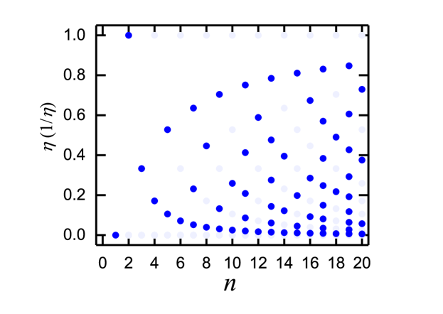
Figure 1: The Relation between the Mass Ratio $\eta$ (or $1/\eta$) and the Collision Times $n$: $\eta=\tan^{2}l\pi/2n$ for Finite Distribution of Momentums

The blue dots represent the solution correspond to the minimum collision times $n$ and pale blue dots represent the repeated solutions. There exists a duality for mass ratio $\eta$ and $1/\eta$.

Given the initial momentum vector, now we explore how many new vectors may come into being after multiple collisions. The reflection matrix allows us to consider only the positive values of the momentum since in the last step one can always invert the sign by applying either $\sigma_{z}$ or $-\sigma_{z}$. In order to effectively study the motion characteristics we may intentionally structure the collision trajectory such that new momentum vector would appear in every pair of scattering-reflection processes. There exist basically two types of trajectories with final momentum vectors expressed as $\left(-1\right)^{m}\left(s\sigma_{z}\right)^{n}\mathbf{k}$ or $\left(-1\right)^{m}\left(\sigma_{z}s\right)^{n}\mathbf{k}$. In the $n$ pairs of scattering-reflection processes, there are $m$ times reflection $-\sigma_{z}$ and $n-m$ times reflection $\sigma_{z}$. Usually, the momentum distribution after multiple collisions becomes rather unpredictable for an arbitrary mass ratio. However, for some special mass ratios, it is possible that after multiple collisions the momentum vector will go back to the initial value. Thus a finite number of momentum vectors form a closed set with the corresponding collision trajectory being a closed loop, which is similar to the fixed point in the regular and chaotic motion of particles bouncing inside a curve [Berry, 1981, Sinai, 1978]. This means that

$$\left(s\left(\eta\right)\sigma_{z}\right)^{n}\left(\begin{array}[]{c}k_{1}\\ k_{2}\end{array}\right)=\pm\left(\begin{array}[]{c}k_{1}\\ k_{2}\end{array}\right)$$ (10)

or

$$\left(\sigma_{z}s\left(\eta\right)\right)^{n}\left(\begin{array}[]{c}k_{1}\\ k_{2}\end{array}\right)=\pm\left(\begin{array}[]{c}k_{1}\\ k_{2}\end{array}\right),$$ (11)

where $\pm$ corresponds even(odd) $m$ respectively.

After some algebras (see transparent method A for details), we find that the above equations (10) and (11) are satisfied if the mass ratio $\eta$ and the number of scattering-reflection pairs $n$, hereafter referred to as collision times, fulfills the following condition

$$\eta=\tan^{2}l\pi/2n,$$ (12)

where $l$ and $n$ are positive integers. For given $\eta$, we aim to find the minimum collision times $n$, after which the momentum sets would be closed. It suffices that let $l$ be any coprime integer to $n$ and $1\leq l\leq n$. There exists a duality for mass ratio $\eta$ and $1/\eta$ and in Fig. 1, we show all qualified mass ratios after $n$-multiple collisions by blue dots, which are two-fold degenerate for $\eta$ and $1/\eta$ except the case of equal mass. A trivial case is that for $\eta=0$ or $1/\eta=0$ which means that there is only one particle left in the hard-wall trap. The closed set contains but one momentum vector as the only collision process is the reflection on the left or right wall, which serves to change it’s sign.

The equation (12) assures that for an given initial momentum vector $\mathbf{k}$ a closed set of finite numbers of the momentum can be obtained by repeatedly applying the scattering and reflection operations on it. In the case of equal mass when $\eta=\tan^{2}\pi/4=1$, the full momentum set is

$$\mathbf{k},r\mathbf{k},r^{2}\mathbf{k},r^{3}\mathbf{k},\sigma_{z}\mathbf{k},r\sigma_{z}\mathbf{k},r^{2}\sigma_{z}\mathbf{k},r^{3}\sigma_{z}\mathbf{k},$$

where $r=s\left(1\right)\sigma_{z}$ and $r^{2}=-I$ with $I$ the $2\times 2$ identity matrix. It is easy to find the collision operators $\left\{I,r,r^{2},r^{3}\right\}$ form a cyclic group $C_{4}$ and $\{I,r,r^{2},r^{3},\sigma_{z},r\sigma_{z},r^{2}\sigma_{z},r^{3}\sigma_{z}\}$ form a dihedral group $D_{4}$. The first nontrivial case arises when $\eta=\tan^{2}\pi/3=3$, and the full momentum set consists of

$$\mathbf{k},r\mathbf{k},r^{2}\mathbf{k},\cdots,r^{5}\mathbf{k},\sigma_{z}\mathbf{k},r\sigma_{z}\mathbf{k},r^{2}\sigma_{z}\mathbf{k},\cdots,r^{5}\sigma_{z}\mathbf{k},$$

where $r=s\left(3\right)\sigma_{z}$ and $r^{3}=-I$. The collision operators $\left\{I,r,r^{2},\cdots,r^{5},\sigma_{z},r\sigma_{z},r^{2}\sigma_{z},\cdots,r^{5}\sigma_{z}\right\}$ form a dihedral group $D_{6}$. Note that when $\eta=\tan^{2}\pi/6=1/3$, the operators $\left\{I,r,r^{2},\cdots,r^{5},\sigma_{z},\right.$ $\left.r\sigma_{z},r^{2}\sigma_{z},\cdots,r^{5}\sigma_{z}\right\}$ with $r=-s\left(1/3\right)\sigma_{z}$ also form a $D_{6}$ group. This again show the duality for mass ratio $\eta$ and $1/\eta$. So we find that Eq.(12) gives a series of classical nonergodicity points and the full momentum set can be written as $\left\{d_{j}\mathbf{k}|d_{j}\in D_{2n}\right\}$. Here the dihedral group $D_{2n}$ with $n=2,3,\cdots$ has $4n$ elements, i.e. $D_{2n}=\left\{I,r,r^{2},\cdots,r^{2n-1},\sigma_{z},r\sigma_{z},\cdots,r^{2n-1}\sigma_{z}\right\}$, where $r=\pm s\left(\eta\right)\sigma_{z}$ and $r^{2n}=I$. Here the sign $+$ and $-$ are for $\eta\geq 1$ and $\eta<1$, respectively.

Table 1: The relationship between mass ratio $\eta$ and the dihedral group.

$\eta$	$n$	$l$	the dihedral group
$0,+\infty$	$1$	$1$	$D_{2}$
$1$	$2$	$1$	$D_{4}$
$1/3$	$3$	$1$	$D_{6}$
$3$	$3$	$2$	$D_{6}$
$3-2\sqrt{2}$	$4$	$1$	$D_{8}$
$3+2\sqrt{2}$	$4$	$3$	$D_{8}$
$1-2/\sqrt{5}$	$5$	$1$	$D_{10}$
$5-2\sqrt{5}$	$5$	$2$	$D_{10}$
$1+2/\sqrt{5}$	$5$	$3$	$D_{10}$
$5+2\sqrt{5}$	$5$	$4$	$D_{10}$
$7-4\sqrt{3}$	$6$	$1$	$D_{12}$
$7+4\sqrt{3}$	$6$	$5$	$D_{12}$
$\vdots$	$\vdots$	$\vdots$	$\vdots$

In table 1, we list all candidates for the mass ratio $\eta$ which fulfills the closeness of scattered momentum vector and the corresponding dihedral group of the collision operators. As $l$ and $n$ are coprime, the value $n$ solely decides the dihedral group $D_{2n}$. For different mass ratio, the number of momentum vector in the closed set determines the order of the dihedral group. In Fig. 2, we show the distribution of momentum in the closed set for $\eta=1$ and $3$, with the emerging $D_{4}$ and $D_{6}$ symmetry, respectively. Each momentum vector is represented by a point in the phase space $\left(k_{1},\sqrt{\eta}k_{2}\right)$ where we rescale $k_{2}$ by a factor $\sqrt{\eta}$ such that all points are distributed on a circle due to the energy conservation. It is straightforward to see that the momentums are distributed on vertices of two 2n-sided polygons, which fulfill the $D_{2n}$ symmetry. To see it more clearly, we represent the $r$-matrix as

$$r=\left(\begin{array}[]{cc}-\cos\frac{l\pi}{n}&\cos\frac{l\pi}{n}-1\\ \cos\frac{l\pi}{n}+1\newline &-\cos\frac{l\pi}{n}\end{array}\right)$$ (13)

which is obtained by inserting the nonergodicity mass ratio $\left(\ref{nonergodicity}\right)$ into $r=s\left(\eta\right)\sigma_{z}$. Then performing a similar transformation on $r$, we get

$$R=UrU^{-1}=\left(\begin{array}[]{cc}\cos\frac{m\pi}{n}&-\sin\frac{m\pi}{n}\\ \sin\frac{m\pi}{n}\newline &\cos\frac{m\pi}{n}\end{array}\right),$$ (14)

where $m=n-l$ and

$$U=\left(\begin{array}[]{cc}1&0\\ 0\newline &\sqrt{\eta}\end{array}\right).$$

Clearly, $R$ is a two-dimensional rotation matrix, and the standard presentation of the dihedral group $D_{2n}$ is given by

$$D_{2n}=\left\{R,\sigma_{z}|R^{2n}=\sigma_{z}^{2}=1,\sigma_{z}R\sigma_{z}^{-1}=R^{-1}\right\}.$$ (15)

Given an initial set of momentums, the other vertices of polygons are decided by applying the symmetry operations of the $D_{2n}$ group.

Although the general mass-imbalance collision problem in the hard-wall trap does not possess discrete symmetries, the momentum distributions in the phase space exhibit the emergent $D_{2n}$ symmetries in the nonergodicity points, which includes $2n$ rotational symmetries and $2n$ reflection symmetries. If the nonergodicity condition (12) is not fulfilled, Eqs. (10) and (11) no longer hold true, and the momentum distribution does not exhibit discrete symmetry. Instead, the momentums shall distribute on the entire circle with the increase of collision times.

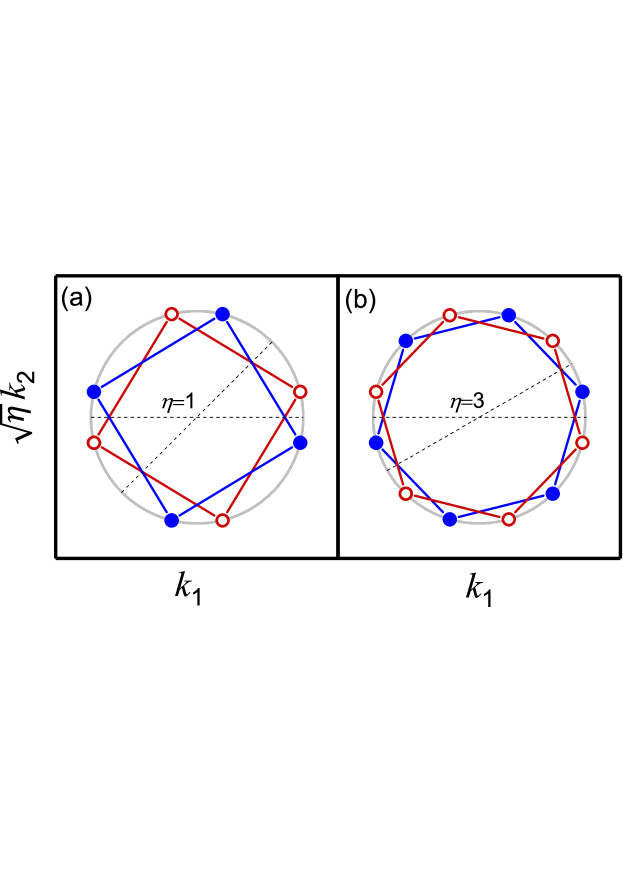
Figure 2: Momentum Distributions of Classical Collision

Momentum distributions in the phase space$\left(k_{1},\sqrt{\eta}k_{2}\right)$ for two particles with mass ratio (a) $\eta=1$ and (b) $\eta=3$, respectively. The momentums are distributed on vertices of two polygons. While vertices on each polygon fulfill $C_{4}$ and $C_{6}$ symmetries for (a) and (b), respectively, vertices on different polygons can be transformed into each other by axial reflection transformations. The dashed lines shown in (a) and (b) are two reflection axes corresponding to axial reflection transformations $\sigma_{z}$ and $R\sigma_{z}$, respectively. (color online.)

SOLVABLE QUANTUM SYSTEM WITH IMBALANCED MASSES

Model and Bethe-type-ansatz solution

Consider a quantum system of two particles with masses $m_{1}$ and $m_{2}$ confined in a 1D hard-wall trap of length $L$. Two atoms interact with each other via the potential $g\delta\left(x_{1}-x_{2}\right)$, where $\delta\left(x\right)$ is the Dirac delta function and $g$ is the interaction strength. The Hamiltonian can be written as

$$H=-\frac{\hbar^{2}}{2m_{1}}\frac{\partial^{2}}{\partial x_{1}^{2}}-\frac{\hbar^{2}}{2m_{2}}\frac{\partial^{2}}{\partial x_{2}^{2}}+g\delta\left(x_{1}-x_{2}\right),$$ (16)

and the wave function $\Psi\left(x_{1},x_{2}\right)$ satisfies the open boundary condition

$$\Psi\left(x_{i}=\pm L/2\right)=0,$$ (17)

for $i=1$ and $2$. The system with equal mass reduces to the well-known solvable Lieb-Liniger model under the open boundary condition [Gaudin, 1971]. If the mass ratio fulfills the nonergodicity condition (12), the number of momentum vectors in the set is finite such that the wavefunction of the quantum system can be taken in terms of Bethe-type hypothesis as

$$\Psi(x_{1},x_{2}) = \theta\left(x_{2}<x_{1}\right)\sum_{j}A_{j+}e^{i\left(d_{j}\mathbf{k}\right)^{T}\mathbf{\cdot x}}$$ (18)

$$+\theta\left(x_{1}<x_{2}\right)\sum_{j}A_{j-}e^{i\left(d_{j}\mathbf{k}\right)^{T}\mathbf{\cdot x}},$$

where $A_{j\pm}$ are the coefficient of plane waves with different quasimomentums and $\theta\left(x\right)$ is the step function. $\mathbf{x}=\left(x_{1},x_{2}\right)^{T}$ and $\mathbf{k}=\left(k_{1},k_{2}\right)^{T}$ are the coordinate vector and the quasimomentum vector of particle $1$ and $2$, respectively, and the collision operator $d_{j}\in D_{2n}$ with $j=1,2,\cdots,4n$. Here $D_{2n}$ is the same dihedral group as in the classical model in previous section. The wave function includes all possible terms in the scattering process with the quasimomentums in the plane waves fulfilling the $D_{2n}$ symmetry. When $\eta=1$, we have $d_{j}\in D_{4}$ and Eq.(18) reduces to the Bethe ansatz wavefuntion of two-particle Lieb-Liniger model under the open boundary condition [Gaudin, 1971]. Although the wavefunction of Eq.(18) is represented in a general form with $d_{j}\in D_{2n}$, in this work we only study the case with $d_{j}\in D_{6}$ corresponding to $\eta=3$ or $1/3$, as we find that it is the only exactly solvable example of quantum mass-imbalance systems with $\eta$ fulfilling the nonergodicity condition Eq.(12). In the following part, we focus on the $\eta=3$ case, which occurs for example in a quantum gas with the formation of trimers with three times of the atomic mass. The case of $\eta=1/3$ can be exactly solved within the same scheme due to the duality relation between $\eta$ and $1/\eta$. For other cases corresponding to irrational $\eta$, we can not find exact solutions by using the Bethe ansatz method. The exact spectrum of the system is given for arbitrary interaction strength.

Firstly we consider the open boundary condition Eq. $\left(\ref{boundry}\right)$. The definition of reflection matrix for particle $1$ on the right wall and on the left wall is

$$R_{j}\left(1,\pm\right)=\frac{A_{j\pm}}{A_{\underline{j}\pm}}=-\exp\left[\mp iL\sum_{l=1,2}d_{j}^{1l}k_{l}\right],$$ (19)

where $\pm$ in $R$ respectively corresponds to the region $x_{2}<x_{1}$ or $x_{1}<x_{2}$, and the superscripts of $d$ indicate the matrix element in the $\left(k_{1},k_{2}\right)^{T}$ space. For convenience, we use $A_{j\pm}$ denotes the coefficients corresponding to the quasimomentum vector $(k_{1}^{\prime},k_{2}^{\prime})=\left(d_{j}\mathbf{k}\right)^{T}$, where, for example, $k_{1}^{\prime}=\sum_{l=1,2}d_{j}^{1l}k_{l}$ denotes the quasimomentum of particle $1$ after collision operator $d_{j}$. We further let ${A_{\underline{j}\pm}}$ represent the coefficients corresponding to the quasimomentum vector $(-k_{1}^{\prime},k_{2}^{\prime})=\left(d_{\underline{j}}\mathbf{k}\right)^{T}$, where

$$d_{\underline{j}}=-\sigma_{z}d_{j},$$ (20)

and the underline of $j$ indicates the reflection of particle $1$. In a similar way, we define the reflection matrix of particle $2$ on the left wall and on the right wall as

$$R_{j}\left(2,\pm\right)=\frac{A_{j\pm}}{A_{\bar{j}\pm}}=-\exp\left[\pm iL\sum_{l=1,2}d_{j}^{2l}k_{l}\right].$$ (21)

Here $A_{\bar{j}\pm}$ represents the coefficients corresponding to the quasimomentum vector $(k_{1}^{\prime},-k_{2}^{\prime})=\left(d_{\bar{j}}\mathbf{k}\right)^{T}$, where

$$d_{\bar{j}}=\sigma_{z}d_{j}$$ (22)

and the overline of $j$ indicates the reflection of particle $2$.

Next we discuss the scattering between two particles. In the relative coordinate the first derivative of wave function is not continuous due to the $\delta$ interaction. We integrate the Schrödinger equation with Hamiltonian $\left(\ref{1}\right)$ from $x=-\varepsilon$ to $x=+\varepsilon$ and then take the limit $\varepsilon\rightarrow 0$. The result is

$$\left[\frac{\partial\Psi}{\partial x}|_{x=0_{+}}-\frac{\partial\Psi}{\partial x}|_{x=0_{-}}\right]-\frac{2\mu}{\hbar^{2}}g\Psi|_{x=0}=0,$$ (23)

where the relative coordinate $x=x_{1}-x_{2}$ and the reduced mass $\mu=m_{1}/\left(\eta+1\right)=m_{1}/4$. Inserting the Bethe-type-ansatz wave function $\left(\ref{wfunction}\right)$ into Eq. $\left(\ref{dis}\right)$, we get the relation

$$i\left(\frac{d_{j}^{11}k_{1}+d_{j}^{12}k_{2}}{1+\eta}-\frac{d_{j}^{21}k_{1}+d_{j}^{22}k_{2}}{1+1/\eta}\right)$$ (24)

$$\times\left(A_{j+}-A_{k+}-A_{j-}+A_{k-}\right)$$

$$= \frac{2\mu}{\hbar^{2}}g\left(A_{j-}+A_{k-}\right),$$

where $A_{j\pm}$ and $A_{k\pm}$ represent the coefficients corresponding to the quasimomentums $\left(d_{j}\mathbf{k}\right)^{T}$ and $\left(d_{k}\mathbf{k}\right)^{T}$, respectively, and the collision operator $d_{j}$ is related to $d_{k}$ via the relation

$$d_{j}=sd_{k}.$$ (25)

On the other hand, for quasimomentum vector $(k_{1}^{\prime},k_{2}^{\prime})=\left(d_{j}\mathbf{k}\right)^{T}$, there always exists $(-k_{1}^{\prime},-k_{2}^{\prime})=\left(-d_{j}\mathbf{k}\right)^{T}$. We denote $d_{\breve{j}}=-d_{j}$ and $d_{\breve{k}}=-d_{k}$, and the corresponding coefficients as $A_{\breve{j}\pm}$ and $A_{\breve{k}\pm}$, which fulfills

$$i\left(\frac{d_{\breve{j}}^{11}k_{1}+d_{\breve{j}}^{12}k_{2}}{1+\eta}-\frac{d_{\breve{j}}^{21}k_{1}+d_{\breve{j}}^{22}k_{2}}{1+1/\eta}\right)$$ (26)

$$\times\left(A_{\breve{j}+}-A_{\breve{k}+}-A_{\breve{j}-}+A_{\breve{k}-}\right)$$

$$= \frac{2\mu}{\hbar^{2}}g\left(A_{\breve{j}-}+A_{\breve{k}-}\right),$$

where $d_{\breve{j}}=sd_{\breve{k}}$ due to Eq. (25). Representing

$$A_{\breve{j}\pm}=T_{j,\pm}A_{j\pm},$$ (27)

we have

$$i\left(-\frac{d_{j}^{11}k_{1}+d_{j}^{12}k_{2}}{1+\eta}+\frac{d_{j}^{21}k_{1}+d_{j}^{22}k_{2}}{1+1/\eta}\right)$$ (28)

$$\times\left(T_{j,+}A_{j+}-T_{k,+}A_{k+}-T_{j,-}A_{j-}+T_{k,-}A_{k-}\right)$$

$$= \frac{2\mu}{\hbar^{2}}g\left(T_{j,-}A_{j-}+T_{k,-}A_{k-}\right).$$

From Eq.(27), Eq.(19) and Eq. $\left(\ref{op2}\right)$, we can get

$$T_{j,\pm}=\exp\left[\mp iL\sum_{l=1,2}\left(d_{j}^{2l}k_{l}-d_{j}^{1l}k_{l}\right)\right],$$ (29)

such that the Eq. $\left(\ref{ds22}\right)$ actually represents the second relation between $A_{j\pm}$ and $A_{k\pm}$.

The continuity of the wavefunction $\Psi|_{x=0_{+}}=\Psi|_{x=0_{-}}$ gives yet another pair of equations

$$A_{j+}+A_{k+}=A_{j-}+A_{k-}$$ (30)

and

$$T_{j,+}A_{j+}+T_{k,+}A_{k+}=T_{j,-}A_{j-}+T_{k,-}A_{k-}.$$ (31)

Obviously the two-particle scattering problem with unequal mass is much more complicated than the equal mass case. For each pair of $k$ and $j$ related by Eq.(25), we have four homogeneous linear equations of four coefficients $A_{j\pm}$ and $A_{k\pm}$, given by Eq. $\left(\ref{ds1}\right)$, $\left(\ref{ds22}\right)$, $\left(\ref{c1}\right)$, and $\left(\ref{c12}\right)$. Non-trivial solution of these coefficients requires the determinant of the corresponding matrix equations to be zero. Since $d_{j}\in D_{6}$, there are altogether $24$ different coefficients and we can get $6$ equations, among which three equations are identical to the other three. This leads to the constraint of the momentum $k_{1}$ and $k_{2}$, which can be shown to be equivalent to either the following pair of Bethe-type-ansatz equations

$$\left\{\begin{array}[]{c}k_{1}+3k_{2}-\frac{2\mu}{\hbar^{2}}g\left(\cot\frac{\left(k_{1}+k_{2}\right)L}{2}+\cot k_{2}L\right)=0,\\ k_{1}-3k_{2}-\frac{2\mu}{\hbar^{2}}g\left(\cot\frac{\left(k_{1}-k_{2}\right)L}{2}-\cot k_{2}L\right)=0,\end{array}\right.$$ (32)

or that of

$$\left\{\begin{array}[]{c}k_{1}+3k_{2}+\frac{2\mu}{\hbar^{2}}g\left(\tan\frac{\left(k_{1}+k_{2}\right)L}{2}+\tan k_{2}L\right)=0,\\ k_{1}-3k_{2}+\frac{2\mu}{\hbar^{2}}g\left(\tan\frac{\left(k_{1}-k_{2}\right)L}{2}-\tan k_{2}L\right)=0.\end{array}\right.$$ (33)

Figure 3: Quasimomentums $k_{1}$ and $k_{2}$ of Quantum System

Quasimomentums $k_{1}$ and $k_{2}$ for the ground state and the first excited state with mass ratio $\eta=3$ for different interaction strengths $\gamma=0.1$, $1$ and $50$. The triangles and squares show the quasimomentums of the ground state and the first excited state, respectively. (color online.)

Here we would like to add a remark for the other mass-imbalanced cases, for example, the case with $\eta=3-2\sqrt{2}$. In this case, we have $d_{j}\in D_{8}$ and there are altogether $32$ different coefficients. By setting the determinant of corresponding matrix equations of Eqs.(24), (28), (30), and (31) to zero, we can get $8$ equations with four of them being identical to the other four. So there are four independent equations with two undetermined variables $k_{1}$ and $k_{2}$, which generally yields no solutions, i.e., it is impossible for $k_{1}$ and $k_{2}$ to fulfill four independent equations simultaneously. This means that the Bethe-type-ansatz wavefunction given by Eq. (18) is not the eigenstate of the mass-imbalanced system with $\eta=3-2\sqrt{2}$. We also verified analytically that for this mass ratio there is no solution in the hard-core interacting case $g\rightarrow+\infty$.

Results and discussions

By numerically solving the transcendental equations $\left(\ref{BA1}\right)$ or $\left(\ref{BA2}\right)$, we can get the quasimomentums for any given interaction $g$. Contrary to the classical model where the momentum can take any continuous values, the quasimomentum here is quantized and can only take discrete values. For convenience, we introduce the dimensionless interaction strength $\gamma=\frac{\mu gL}{\hbar^{2}}$ and adopt the natural units $\hbar=\mu=L=1$. In Fig. 3, we display the solution of quasimomentums for different $\gamma$ when the system is in the ground state and the first excited state. For a finite $\gamma$, the quasimomentums in the figure can be generally classified into three groups, denoted as $(\pm k_{1},\pm k_{2})$, $(\pm k_{1}^{\prime},\pm k_{2}^{\prime})$, and $(\pm k_{1}^{\prime\prime},\pm k_{2}^{\prime\prime})$, respectively. The phase space can be divided into four quadrants and every quadrant is sprinkled with three points. The points in the first quadrant are related to those in other quadrants by the reflection operators $\sigma_{z}$, $-\sigma_{z}$ and $-I$. Thus we focus on the three points in first quadrant: $\mathbf{k}=(k_{1},k_{2})^{T}$, $\mathbf{k}^{\prime}=(k_{1}^{\prime},k_{2}^{\prime})^{T}$ and $\mathbf{k}^{\prime\prime}=(k_{1}^{\prime\prime},k_{2}^{\prime\prime})^{T}$. Once we find a solution $\mathbf{k}$ from the Bethe-type-ansatz equations, it is easy to obtain $\mathbf{k}^{\prime}$ and $\mathbf{k}^{\prime\prime}$ by applying appropraite group operators on $\mathbf{k}$, which necessarily fulfill the same equations. Take the ground state for $\gamma=1$ in Fig. 3(b) as an example. From $\mathbf{k}=(0.93667\pi,1.17904\pi)^{T}$, one immediately knows that $\mathbf{k}^{\prime}=-\sigma_{z}s\sigma_{z}\mathbf{k}=(1.30023\pi,1.05786\pi)^{T}$ and $\mathbf{k}^{\prime\prime}=\sigma_{z}s\mathbf{k}=(2.2369\pi,0.12119\pi)^{T}$ are all the solution of Bethe-type-ansatz equations $\left(\ref{BA1}\right)$.

Particularly, when $\gamma\rightarrow 0$, we find every two points of momentum in the ground state tend to be the same and $1/3$ of the points will be located on the straight line $k_{2}=0$. Note that for the non-interacting case, the transcendental equations $\left(\ref{BA1}\right)$ reduces to

$$\left\{\begin{array}[]{c}\cot\frac{k_{1}+k_{2}}{2}+\cot k_{2}=\infty,\\ \cot\frac{k_{1}-k_{2}}{2}-\cot k_{2}=\infty,\end{array}\right.$$ (34)

which leads to the single particle solution: $k_{1}=n_{1}\pi$, $k_{2}=n_{2}\pi$, where $n_{1}$ and $n_{2}$ are integers. The quantum numbers of the ground state is $(n_{1},n_{2})=(1,1)$ and the corresponding energy is $\pi^{2}/2$. We find that $\mathbf{k}=\mathbf{k}^{\prime}=(\pi,\pi)^{T}$ are equal, which holds for all other cases with $n_{1}=n_{2}$. The coefficients for the plane waves with $\mathbf{k}^{\prime\prime}=(2\pi,0)^{T}$, however, are vanishing in the non-interacting case and the wave function is but the direct product state of the two single-particle ground states. The plane waves with approximately $(\pm 2\pi,0)$, i.e. the four points near the $k_{2}$ axis, prove to be emergent solutions uniquely in the weakly interacting case, as the wave function of zero momentum, that is, a constant, violates the vanishing condition at both left and right boundaries in the non-interacting case. More emergent solutions like these are found for the excited states, which are prohibited in the non-interacting case and yet contribute in the superposition of Bethe-type hypothesis of the interacting many-body wave function. For instance, the emergent solutions for the first excited state corresponding to $(n_{1},n_{2})=(2,1)$ with approximate energy $7\pi^{2}/8$ are plane waves with the momentum taking the values near half-integer-multiple of $\pi$, specifically, $\mathbf{k}^{\prime}\approx(5\pi/2,\pi/2)^{T}$, $\mathbf{k}^{\prime\prime}\approx(\pi/2,3\pi/2)^{T}$. This is an intrinsic feature for the mass-imbalanced system as we have noticed that no solutions emerge in the equal mass case.

On the other hand, when $\gamma\rightarrow\infty$, the ground state and the first excited state tend to be degenerate. In this case the transcendental equations $\left(\ref{BA1}\right)$ reduce to

$$\left\{\begin{array}[]{c}\cot\frac{k_{1}+k_{2}}{2}+\cot k_{2}=0,\\ \cot\frac{k_{1}-k_{2}}{2}-\cot k_{2}=0.\end{array}\right.$$ (35)

From the above equations, it follows that $k_{1}=n_{1}\pi$ and $k_{2}=n_{2}\pi/3$ with $n_{1}$ and $n_{2}$ being integers. The symmetry in the quasi-momentum set, however, constraints the values of $n_{1}$ and $n_{2}$ to some specific integers. This can be understood as following: in the momentum set, not only $\mathbf{k}$, but also $\mathbf{k}^{\prime}$ and $\mathbf{k}^{\prime\prime}$, which are related by collision operators in the group $D_{6}$, necessarily satisfy the above equations. For example, when $n_{1}=1$, $n_{2}=1$, the momentum values $\mathbf{k}^{\prime}=s\sigma_{z}\mathbf{k}=(0,2\pi/3)^{T}$ violate the equations (35), while $n_{1}=1$, $n_{2}=2$, $\mathbf{k}^{\prime}=s\mathbf{k}=(3\pi/2,\pi/6)^{T}$ again fail them, etc. It can be shown when $n_{1}=1$, the minimum value of $n_{2}$ to satisfy (35) is $n_{2}=5$. So the lowest values for the quasimomentum are $\mathbf{k}=(\pi,5\pi/3)^{T}$, $\mathbf{k}^{\prime}=(2\pi,4\pi/3)^{T}$ and $\mathbf{k}^{\prime\prime}=(3\pi,\pi/3)^{T}$. In the infinitely interacting case, the ground state and the first excited state are degenerate with eigenenergy $7\pi^{2}/6$ which is a little bit larger than the first excited state energy of the non-interacting case. The solutions at these two limits are consistent with the alternative analysis in the transparent method B.

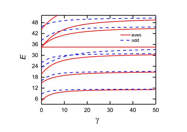
Figure 4: Energy Spectrum of Two Atoms with Mass Ratio $\eta=3$ in the Hard-wall Trap as a Function of the Interaction Strength $\gamma$

The red solid lines show the eigenstates with even parity and the blue dashed lines with odd parity. (color online.)

The finite interaction case interpolates between these two limits as shown in Fig. $3$. We find that the momentum points in the weak interaction case $\gamma=0.1$ are very close to the free particle case $\gamma=0$. Nevertheless, the heavy and light particles in the interacting case are entangled and the wave function is no longer a product state. The quasimomentum points for the ground state occupy the vertices of two regular hexagons on a circle in the phase space $(k_{1},\sqrt{3}k_{2})$, while the overlapped points in the free particle case start to be split into two when the interaction gradually sets in. The ground state circle then expands towards that of the first excited state with the increase of the interaction strength and finally join it in the infinitely interacting case, leading to the degeneracy of the two states, which is already clearly seen for $\gamma=50$ as shown in Fig. $3$(c).

In Fig. $4$, we plot the energy spectrum $E=(k_{1}^{2}+3k_{2}^{2})/8$ as a function of the interaction $\gamma$. We find that every energy level corresponds to a fixed parity, as the corresponding wavefunction fulfills the parity symmetry:

$$\Psi(x_{1},x_{2})=\pm\Psi(-x_{1},-x_{2}),$$ (36)

where the even parity is with sign ”$+$” and odd parity with ”$-$”. With the increase of $\gamma$, the eigenvalues generally increase except for some special states, e.g., the seventh excited state as shown in Fig. 5 does not change with $\gamma$. In the limit case $\gamma=\infty$, two levels with opposite parity tend to be doubly degenerate, and the wave functions vanish along the line $x_{1}=x_{2}$.

We note that the seventh excited state is an even parity state whose energy is independent of the interaction strength. The existence of such a state is related to the emergence of a triple degenerate point in the noninteracting limit $\gamma=0$. These three degenerate states are labeled by quantum numbers $(n_{1},n_{2})=(5,1)$, $(4,2)$, and $(1,3)$, respectively, which have no correspondence in the equal mass case. In the presence of interaction, the triple degeneracy is usually broken. Nevertheless, we can construct a wavefunction composed of a superposition of triple degenerate eigenstates, which is the eigenstate of the interacting Hamiltonian with eigenvalue irrelevant to the interaction strength. Explicitly, the wavefunction of this state is given by

$$\Psi(x_{1},x_{2}) = \frac{1}{\sqrt{3}}[\phi_{5}(x_{1})\phi_{1}(x_{2})$$ (37)

$$-\phi_{4}(x_{1})\phi_{2}(x_{2})+\phi_{1}(x_{1})\phi_{3}(x_{2})],$$

where

$$\phi_{n}\left(x\right)=\sqrt{\frac{2}{L}}\sin\frac{n\pi}{L}\left(\frac{L}{2}+x\right)$$

is the $n$-th single-particle eigenstate of the hard well. After some straightforward algebras, it is easy to check that $\Psi(x_{1},x_{2})|_{x_{1}=x_{2}}=0$, i.e., the wavefunction takes zero at $x_{1}=x_{2}$, indicating that the state given by Eq. (37) is the eigenstate of Hamiltonian (16) irrelevant to the value of $\gamma$. Actually, there are a series of such excited states, corresponding to the higher triple degenerate points in the noninteracting limit. Generally, triple degenerate states are characterized by the quantum numbers $(n_{1},n_{2})$, which should fulfill three conditions, i.e., $n_{1}+n_{2}$ is even, $n_{1}\neq n_{2}$ and $n_{1}\neq 3n_{2}$. The corresponding wavefunction can be written as

$$\Psi(x_{1},x_{2}) = \frac{1}{\sqrt{3}}[\phi_{n_{1}}(x_{1})\phi_{n_{2}}(x_{2})$$

$$\pm\phi_{n_{1}^{\prime}}(x_{1})\phi_{n_{2}^{\prime}}(x_{2})\pm\phi_{n_{1}^{\prime\prime}}(x_{1})\phi_{n_{2}^{\prime\prime}}(x_{2})],$$

where the selections of $"\pm"$ depend on the concrete values of quantum numbers $n_{1}$ and $n_{2}$. An example for the next excited state, independent of $\gamma$, is labeled by quantum numbers $(n_{1},n_{2})=(2,4)$, $(n_{1}^{\prime},n_{2}^{\prime})=(7,1)$, and $(n_{1}^{\prime\prime},n_{2}^{\prime\prime})=(5,3)$.

In Fig. $5$, we display the probability density distribution $\rho\left(x_{1},x_{2}\right)=\left|\Psi(x_{1},x_{2})\right|^{2}$ for the ground state and the first excited state as well as the seventh excited state with three typical interaction strength parameters $\gamma=0.1,1,10$. Comparing to the equal mass case, the two-body wavefunction no longer has exchange symmetry, nevertheless it keeps the parity symmetry. It is obvious that the density distribution fulfills $\rho\left(-x_{1},-x_{2}\right)=\rho\left(x_{1},x_{2}\right)$. We find that with the interaction increased, particles will avoid to occupy the same position and the density along the diagonal line $x_{1}=x_{2}$ is greatly suppressed. In the strong interaction region, the density of the ground and first excited states exhibit almost the same density patterns. In the infinitely repulsive limit, the densities for the degenerate states are exactly same with zero distribution along the diagonal line. For the seventh excited state, it is clear that the density distribution is independent of $\gamma$ and always gives zero along the diagonal line.

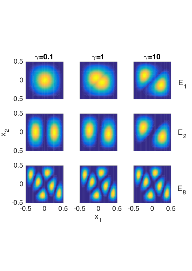
Figure 5: The Normalized Probability Density $\rho\left(x_{1},x_{2}\right)$ for Two Unequal Mass Particles in the Hard-wall Trap

The columns represent results for three interaction parameters $\gamma=0.1$, $1$ and $10$, respectively. The rows from top to bottom are for the ground state, the first and the $7$-th excited state, respectively. (color online.)

In summary, we study the problem of two interacting particles with unequal masses in a hard-wall trap and unveil that the system is exactly solvable by using Bethe-type ansatz only for the mass ratio $\eta=3$ or $1/3$. Since the Bethe-type ansatz is based on the wavefunction hypothesis which requires finite superpositions of plane waves, the solvability of the mass-imbalance quantum system is thus related to a problem of seeking nonergodicity conditions in the classical elastic collision in a 1D hard-wall trap. In general, each collision and reflection process of two particles with unequal masses gives rise to a new set of momentums $k_{1}$ and $k_{2}$, which shall not form finite momentum distributions after multiple collisions. Nevertheless, we find that finite momentum distributions after multiple collisions are available at specific values of mass ratio, which is determined by the nonergodicity condition. For $\eta=3$ or $1/3$, the permitted momentums fulfill the $D_{6}$ symmetry. Based on the Bethe-type ansatz, we then exactly solve the quantum system with mass ratio $3$ and give Bethe-type-ansatz equations for arbitrary interaction strength. By solving the Bethe-type-ansatz equations, we give the energy spectrum and wavefunctions of the mass-imbalance system with $\eta=3$, which are found to display some peculiar behaviors with no correspondence in the equal-mass system.

Limitation of the Study

Although nonergodicity condition for the classical collision problem in a hard-wall trap includes a series of solutions of mass ratio, the extended Bethe ansatz method can only give the exact solution for the two-particle quantum system with the mass ratio $\eta=3$ or $1/3$. Our method can not be directly applied to solve the three-particle system. The properties of many-particle interacting models with unequal masses are still not clear and worth further investigating.

Methods

All methods can be found in the accompanying Transparent Methods supplemental file.

Supplemental information

Supplemental Information includes Transparent Methods.

Author contributions

Y.Z. and S. C. conceived the project and supervised the study. Y.L. and F.Q. performed the numerical calculations and theoretical analysis. Y.L., Y.Z., and S. C. contributed to writing the manuscript.

Declaration of interests

The authors declare no competing interests.

References

Supplemental Information

Transparent Methods

A. Solution to equations for nonergodicity condition

Here we show the derivation of the nonergodicity condition

$$\eta=\tan^{2}l\pi/2n,$$ (S38)

by solving the equations

$$\left(s\left(\eta\right)\sigma_{z}\right)^{n}\left(\begin{array}[]{c}k_{1}\\ k_{2}\end{array}\right)=\pm\left(\begin{array}[]{c}k_{1}\\ k_{2}\end{array}\right)$$ (S39)

and

$$\left(\sigma_{z}s\left(\eta\right)\right)^{n}\left(\begin{array}[]{c}k_{1}\\ k_{2}\end{array}\right)=\pm\left(\begin{array}[]{c}k_{1}\\ k_{2}\end{array}\right).$$ (S40)

A quite useful tool, Chebyshev identity, is used to derive the relation for the matrix elements of the $n$th power of the matrix.

Consider a unimodular matrix $\mathbf{M}$ given by

$$\mathbf{M}=\left(\begin{array}[]{cc}a&b\\ c&d\end{array}\right),$$ (S41)

where $\text{Det}\mathbf{M}=ad-bc=1$. Suppose that eigenvalues of the unimodular matrix $\mathbf{M}$ are given by

$$\lambda_{1}=e^{iq}\text{ and }\lambda_{2}=e^{-iq},\text{ }$$ (S42)

then the $n$-th power of the matrix $\mathbf{M}$ can be represented as [Yeh et al., 1977]

$$\mathbf{M}^{n}=\left(\begin{array}[]{cc}a&b\\ c&d\end{array}\right)^{n}\\ =\left(\begin{array}[]{cc}aU_{n-1}-U_{n-2}&bU_{n-1}\\ cU_{n-1}&dU_{n-1}-U_{n-2}\end{array}\right),$$ (S43)

where the function $U_{n}$ is defined as

$$U_{n}=\frac{\sin\left(n+1\right)q}{\sin q},$$ (S44)

and $q$ is given by the eigenvalues of the matrix $\mathbf{M}$ via the relation

$$Tr\mathbf{M=}\lambda_{1}+\lambda_{2}=2\cos q.$$ (S45)

The details for the derivation of the Chebyshev identity Eq. (S43) can be found in Ref. [Yeh et al., 1977].

Now we let

$$\mathbf{M=}s\left(\eta\right)\sigma_{z}=\left(\begin{array}[]{cc}\frac{\eta-1}{\eta+1}&\frac{-2\eta}{\eta+1}\\ \frac{2}{\eta+1}&\frac{\eta-1}{\eta+1}\end{array}\right)$$ (S46)

and

$$\mathbf{M}^{\prime}\mathbf{=}\sigma_{z}s\left(\eta\right)=\left(\begin{array}[]{cc}\frac{\eta-1}{\eta+1}&\frac{2\eta}{\eta+1}\\ \frac{-2}{\eta+1}&\frac{\eta-1}{\eta+1}\end{array}\right).$$ (S47)

It is easy to check $\text{Det}\mathbf{M}=\text{Det}\mathbf{M}^{\prime}=1$. Comparing $\mathbf{M}$ and $\mathbf{M}^{\prime}$, we find that the diagonal terms are the same, i.e. $\mathbf{M}_{11}=\mathbf{M}_{11}^{\prime}$, $\mathbf{M}_{22}=\mathbf{M}_{22}^{\prime}$ and off-diagonal terms are opposite numbers with each other, i.e. $\mathbf{M}_{12}=-\mathbf{M}_{12}^{\prime}$, $\mathbf{M}_{21}=-\mathbf{M}_{21}^{\prime}$. So the eigenvalues for two matrices are the same and can be represented as

$$\lambda_{1,2}=\frac{\eta-1\pm 2\sqrt{-\eta}}{\eta+1}.$$ (S48)

From (S45), we can get the relation

$$\cos q=\frac{\eta-1}{\eta+1}.$$ (S49)

To solve the equation (S39) or (S40) is equivalent to solve

$$\left(\mathbf{M}\right)^{n}=\pm\left(\begin{array}[]{cc}1&0\\ 0&1\end{array}\right)$$ (S50)

or

$$\left(\mathbf{M}^{\prime}\right)^{n}=\pm\left(\begin{array}[]{cc}1&0\\ 0&1\end{array}\right).$$ (S51)

Using the Chebyshev identity (S43), we can find that $\left(\mathbf{M}^{n}\right)_{11}=\left(\mathbf{M}^{n}\right)_{22}=\left(\mathbf{M}^{\prime n}\right)_{11}=\left(\mathbf{M}^{\prime n}\right)_{22}$. The solutions of $\mathbf{M}$ and $\mathbf{M}^{\prime}$ satisfy the same relation

$$\left(\mathbf{M}^{n}\right)_{11}=\pm 1,$$

this is

$$\frac{\eta-1}{\eta+1}U_{n-1}-U_{n-2}=\cos nq=\pm 1.$$ (S52)

The solutions of (S52) are

$$q=\frac{l\pi}{n},l=1,2,3\cdots.$$

Then we can also get

$$U_{n-1}=\frac{\sin nq}{\sin q}=0,$$

which ensures that the off-diagonal terms of $\mathbf{M}$ and $\mathbf{M}^{\prime}$ are $0$. Solving the equation (S49), we get

$$\eta=\frac{1+\cos q}{1-\cos q}=\frac{1}{\tan^{2}\frac{l\pi}{2n}},l=1,2,3\cdots.$$ (S53)

Because $l$ and $n$ are both integers, (S53) can be written as other form

$$\eta=\frac{1}{\tan^{2}\frac{\left(n-l\right)\pi}{2n}}=\tan^{2}\frac{l\pi}{2n},l=1,2,3\cdots.$$

The solutions requires that the diagonal terms of matrix $\mathbf{M}^{n}$($\mathbf{M}^{\prime n}$) equal $\pm 1$ and off-diagonal terms equal $0$, so the sign of the off-diagonal do not affect the solutions.

B. The hard-core limit and $g=0$ limit

We consider two limit cases. The first case is the hard-core limit with $g=\infty$, in which the wave function satisfies the boundary condition

$$\Psi|_{x_{1}=x_{2}}=0.$$

Inserting the Bethe-type wave function into the above equation, we get a pair of equations:

$$A_{j\pm}=-A_{k\pm},d_{j}=sd_{k}$$ (S54)

and

$$T_{j,\pm}A_{j\pm}=-T_{k,\pm}A_{k\pm}.$$ (S55)

Combining Eq. (S54) with Eq. (S55), we get the relation

$$\frac{T_{j,-}}{T_{k,-}}=1,$$

i.e.,

$$\exp\left(iL\sum_{l=1,2}3d_{j}^{2l}k_{l}-iL\sum_{l=1,2}d_{j}^{1l}k_{l}\right)=1,$$

which gives rise to three independent equations:

$$\exp\left[iL\left(3k_{2}-k_{1}\right)\right] = 1,$$

$$\exp\left[iL\left(3k_{2}+k_{1}\right)\right] = 1,$$

$$\exp\left[2iLk_{1}\right] = 1.$$

By solving the above equations, we can get a series of solution $k_{1}=l_{1}\pi/L$ and $k_{2}=l_{2}\pi/3L$, where $l_{1}$ and $l_{2}$ are integers and some of them are redundant. Given that $\mathbf{k}=\left(k_{1},k_{2}\right)^{T}$ is a solution of the above transcendental equations, all the quasimomentums obtained via $d_{j}\mathbf{k}$ should also be the solution of transcendental equations, which gives some restrictions to the values of $l_{1}$ and $l_{2}$. According to the ratio relations of the coefficients described by reflection matrixes and Eq. (S54), the wavefunction can be written as

$$\Psi(x_{1},x_{2}) = \theta\left(x_{2}<x_{1}\right)[\Phi_{\mathbf{k}}(x_{1},x_{2})$$

$$-\Phi_{\mathbf{k}^{\prime}}(x_{1},x_{2})+e^{-ik_{2}L}\Phi_{\mathbf{k}^{\prime\prime}}(x_{1},x_{2})]$$

$$\pm\theta\left(x_{1}<x_{2}\right)[\Phi_{\mathbf{k}}(-x_{1},-x_{2})$$

$$-\Phi_{\mathbf{k}^{\prime}}(-x_{1},-x_{2})+e^{-ik_{2}L}\Phi_{\mathbf{k}^{\prime\prime}}(-x_{1},-x_{2})]$$

where $\mathbf{k}^{\prime}=s\mathbf{k}$, $\mathbf{k}^{\prime\prime}=s\sigma_{z}\mathbf{k}$ and

$$\Phi_{\mathbf{k}}(x_{1},x_{2})$$ (S56)

$$= e^{i\left(k_{1}x_{1}+k_{2}x_{2}\right)}-e^{-ik_{2}L}e^{i\left(k_{1}x_{1}-k_{2}x_{2}\right)}$$

$$-e^{ik_{1}L}e^{i\left(-k_{1}x_{1}+k_{2}x_{2}\right)}+e^{-ik_{2}L+ik_{1}L}e^{i\left(-k_{1}x_{1}+k_{2}x_{2}\right)}$$

$$= 4e^{-i\frac{k_{1}+k_{2}}{2}L}\sin k_{1}\left(\frac{L}{2}-x_{1}\right)\sin k_{2}\left(\frac{L}{2}+x_{2}\right).$$

It is interesting to note that two mass-imbalance hard-core particles moving in a 1D box is equivalent to a triangle billiard system [Zhang et al., 2016, Wang et al., 2014, Gorin, 2001], and thus our exact result is helpful for understanding quantum billiard systems from a different perspective.

The other case is the non-interacting limit with $g=0$. In this limit, we have $k_{1}=n_{1}\pi/L$ and $k_{2}=n_{2}\pi/L$, where $n_{1}$ and $n_{2}$ are integers. Since the system is composed of particles with different masses, the wavefunction can be written as a product state of two single-particle wavefunctions

$$\Psi(x_{1},x_{2})=\phi_{n_{1}}(x_{1})\phi_{n_{2}}(x_{2}),$$

where

$$\phi_{n}\left(x\right)=\sqrt{\frac{2}{L}}\sin\frac{n\pi}{L}\left(\frac{L}{2}+x\right)$$

is the eigenstate of the 1D hard-wall potential.

References

- Albeverio and Holden [1988] Albeverio, S., G.F.H.K.R., Holden, H., 1988. Solvable Models in Quantum Mechanics. Springer-Verlag, Berlin.
- Batchelor et al. [2005] Batchelor, M.T., Guan, X.W., Oelkers, N., Lee, C., 2005. The 1d interacting bose gas in a hard wall box. J. Phys. A 38, 7787–7806. doi:10.1088/0305-4470/38/36/001.
- Berry [1981] Berry, M.V., 1981. Regularity and chaos in classical mechanics illustrated by three deformations of a circular billiard. Eur. J. Phys 2, 91–102. doi:10.1088/0143-0807/2/2/006.
- Busch et al. [1998] Busch, T., Englert, B.G., Rzażewski, K., Wilkens, M., 1998. Two cold atoms in a harmonic trap. Found. Phys. 28, 549–559. doi:10.1023/a:1018705520999.
- Chen et al. [2011] Chen, X., Guan, L.M., Chen, S., 2011. Analytical solutions for two heteronuclear atoms in a ring trap. Eur. Phys. J. D 64, 459–464. doi:10.1140/epjd/e2011-20201-6.
- Chin et al. [2010] Chin, C., Grimm, R., Julienne, P., Tiesinga, E., 2010. Feshbach resonances in ultracold gases. Rev. Mod. Phys 82, 1225–1286. doi:10.1103/revmodphys.82.1225.
- Dehkharghani et al. [2016] Dehkharghani, A.S., Volosniev, A.G., Zinner, N.T., 2016. Impenetrable mass-imbalanced particles in one-dimensional harmonic traps. J. Phys. B: At. Mol. Opt. Phys. 49, 085301. doi:10.1088/0953-4075/49/8/085301.
- Deuretzbacher et al. [2008] Deuretzbacher, F., Plassmeier, K., Pfannkuche, D., Werner, F., Ospelkaus, C., Ospelkaus, S., Sengstock, K., Bongs, K., 2008. Heteronuclear molecules in an optical lattice: Theory and experiment. Phys. Rev. A 77, 032726. doi:10.1103/physreva.77.032726.
- Evans [1990] Evans, N.W., 1990. Superintegrability in classical mechanics. Phys. Rev. A 41, 5666–5676. doi:10.1103/physreva.41.5666.
- Ferrier-Barbut et al. [2014] Ferrier-Barbut, I., Delehaye, M., Laurent, S., Grier, A.T., Pierce, M., Rem, B.S., Chevy, F., Salomon, C., 2014. A mixture of bose and fermi superfluids. Science 345, 1035–1038. doi:10.1126/science.1255380.
- Gaudin [1971] Gaudin, M., 1971. Boundary energy of a bose gas in one dimension. Phys. Rev. A 4, 386–394. doi:10.1103/physreva.4.386.
- Gaudin [2014] Gaudin, M., 2014. The Bethe Wavefunction. Cambridge University Press, Cambridge.
- Gutkin [1982] Gutkin, E., 1982. Integrable systems with delta-potential. Duke Math. J. 49, 1–21. doi:10.1215/s0012-7094-82-04901-8.
- Hao et al. [2006] Hao, Y., Zhang, Y., Liang, J.Q., Chen, S., 2006. Ground-state properties of one-dimensional ultracold bose gases in a hard-wall trap. Phys. Rev. A 73, 063617. doi:10.1103/physreva.73.063617.
- Harshman et al. [2017] Harshman, N., Olshanii, M., Dehkharghani, A., Volosniev, A., Jackson, S.G., Zinner, N., 2017. Integrable families of hard-core particles with unequal masses in a one-dimensional harmonic trap. Phys. Rev. X 7, 041001. doi:10.1103/physrevx.7.041001.
- Lieb and Liniger [1963] Lieb, E.H., Liniger, W., 1963. Exact analysis of an interacting bose gas. i. the general solution and the ground state. Phys. Rev. 130, 1605–1616. doi:10.1103/physrev.130.1605.
- McGuire [1964] McGuire, J.B., 1964. Study of exactly soluble one-dimensional n-body problems. J. Math. Phys. 5, 622–636. doi:10.1063/1.1704156.
- Murmann et al. [2015a] Murmann, S., Bergschneider, A., Klinkhamer, V.M., Zürn, G., Lompe, T., Jochim, S., 2015a. Two fermions in a double well: Exploring a fundamental building block of the hubbard model. Phys. Rev. Lett. 114, 080402. doi:10.1103/physrevlett.114.080402.
- Murmann et al. [2015b] Murmann, S., Deuretzbacher, F., Zürn, G., Bjerlin, J., Reimann, S., Santos, L., Lompe, T., Jochim, S., 2015b. Antiferromagnetic heisenberg spin chain of a few cold atoms in a one-dimensional trap. Phys. Rev. Lett. 115, 215301. doi:10.1103/physrevlett.115.215301.
- Olshanii and Jackson [2015] Olshanii, M., Jackson, S.G., 2015. An exactly solvable quantum four-body problem associated with the symmetries of an octacube. New J. Phys. 17, 105005. doi:10.1088/1367-2630/17/10/105005.
- Olshanii et al. [2018] Olshanii, M., Scoquart, T., Yampolsky, D., Dunjko, V., Jackson, S.G., 2018. Creating entanglement using integrals of motion. Phys. Rev. A 97, 013630. doi:10.1103/physreva.97.013630.
- Pecak et al. [2016] Pecak, D., Gajda, M., Sowiński, T., 2016. Two-flavour mixture of a few fermions of different mass in a one-dimensional harmonic trap. New J. Phys. 18, 013030. doi:10.1088/1367-2630/18/1/013030.
- Pecak and Sowiński [2016] Pecak, D., Sowiński, T., 2016. Few strongly interacting ultracold fermions in one-dimensional traps of different shapes. Phys. Rev. A 94, 042118. doi:10.1103/physreva.94.042118.
- Post et al. [2012] Post, S., Tsujimoto, S., Vinet, L., 2012. Families of superintegrable hamiltonians constructed from exceptional polynomials. J. Phys. A: Math. Theor. 45, 405202. doi:10.1088/1751-8113/45/40/405202.
- Richens and Berry [1981] Richens, P., Berry, M., 1981. Pseudointegrable systems in classical and quantum mechanics. Physica D: Nonlinear Phenomena 2, 495–512. doi:10.1016/0167-2789(81)90024-5.
- Scoquart et al. [2016] Scoquart, T., Seaward, J., Jackson, S.G., Olshanii, M., 2016. Exactly solvable quantum few-body systems associated with the symmetries of the three-dimensional and four-dimensional icosahedra. SciPost Phys. 1, 005. doi:10.21468/scipostphys.1.1.005.
- Serwane et al. [2011] Serwane, F., Zurn, G., Lompe, T., Ottenstein, T.B., Wenz, A.N., Jochim, S., 2011. Deterministic preparation of a tunable few-fermion system. Science 332, 336–338. doi:10.1126/science.1201351.
- Sinai [1978] Sinai, Y., 1978. Introduction to Ergodic Theory. Princeton University Press, Princeton.
- Sutherland [1968] Sutherland, B., 1968. Further results for the many-body problem in one dimension. Phys. Rev. Lett. 20, 98–100. doi:10.1103/physrevlett.20.98.
- Sutherland [2004] Sutherland, B., 2004. Beautiful Models: 70 Years of Exactly Solved Quantum Many-Body Problems. World Scientific, Singapore.
- Takahashi [1999] Takahashi, M., 1999. Thermodynamics of One-Dimensional Solvable Models. Cambridge University Press, Cambridge.
- Tempesta et al. [2001] Tempesta, P., Turbiner, A.V., Winternitz, P., 2001. Exact solvability of superintegrable systems. J. Math. Phys. 42, 4248–4257. doi:10.1063/1.1386927.
- Volosniev [2017] Volosniev, A.G., 2017. Strongly interacting one-dimensional systems with small mass imbalance. Few-Body Systems 58, 54. doi:10.1007/s00601-017-1227-0.
- Wenz et al. [2013] Wenz, A.N., Zurn, G., Murmann, S., Brouzos, I., Lompe, T., Jochim, S., 2013. From few to many: Observing the formation of a fermi sea one atom at a time. Science 342, 457–460. doi:10.1126/science.1240516.
- Yang [1967] Yang, C.N., 1967. Some exact results for the many-body problem in one dimension with repulsive delta-function interaction. Phys. Rev. Let. 19, 1312–1315. doi:10.1103/physrevlett.19.1312.
- Yao et al. [2016] Yao, X.C., Chen, H.Z., Wu, Y.P., Liu, X.P., Wang, X.Q., Jiang, X., Deng, Y., Chen, Y.A., Pan, J.W., 2016. Observation of coupled vortex lattices in a mass-imbalance bose and fermi superfluid mixture. Phys. Rev. Lett. 117, 145301. doi:10.1103/physrevlett.117.145301.
- Zürn et al. [2012] Zürn, G., Serwane, F., Lompe, T., Wenz, A.N., Ries, M.G., Bohn, J.E., Jochim, S., 2012. Fermionization of two distinguishable fermions. Phys. Rev. Lett. 108, 075303. doi:10.1103/physrevlett.108.075303.
- Zürn et al. [2013] Zürn, G., Wenz, A.N., Murmann, S., Bergschneider, A., Lompe, T., Jochim, S., 2013. Pairing in few-fermion systems with attractive interactions. Phys. Rev. Lett. 111, 175302. doi:10.1103/physrevlett.111.175302.

References

- Gorin [2001] Gorin, T., 2001. Generic spectral properties of right triangle billiards. Journal of Physics A: Mathematical and General 34, 8281–8295. doi:10.1088/0305-4470/34/40/306.
- Wang et al. [2014] Wang, J., Casati, G., Prosen, T., 2014. Nonergodicity and localization of invariant measure for two colliding masses. Physical Review E 89, 042918. doi:10.1103/physreve.89.042918.
- Yeh et al. [1977] Yeh, P., Yariv, A., Hong, C.S., 1977. Electromagnetic propagation in periodic stratified media i. general theory. Journal of the Optical Society of America 67, 423. doi:10.1364/josa.67.000423.
- Zhang et al. [2016] Zhang, D., Quan, H.T., Wu, B., 2016. Ergodicity and mixing in quantum dynamics. Physical Review E 94, 022150. doi:10.1103/physreve.94.022150.