On the Rayleigh-Taylor unstable dynamics of 3D interfacial coherent
structures with time-dependent acceleration

Abstract

Rayleigh-Taylor instability (RTI) occurs in a range of industrial and natural processes. Whereas the vast majority of existing studies have considered constant acceleration, RTI is in most instances driven by variable acceleration. Here we focus on RTI driven by acceleration with a power-law time-dependence, and by applying a group theoretic method find solutions to this classical nonlinear boundary value problem. We deduce that the dynamics is dominated by the acceleration term and that the solutions depend critically on the time dependence for values of the acceleration exponent greater than $-2$. We find that in the early-time dynamics, the RTI growth-rate depends on the acceleration parameters and initial conditions. For the later-time dynamics, we link the interface dynamics with an interfacial shear function, and find a continuous family of regular asymptotic solutions and invariant properties of nonlinear RTI. The essentially interfacial and multi-scale character of the dynamics is also demonstrated. The velocity field is potential in the bulk, and vortical structures appear at the interface due to interfacial shear. The multi-scale character becomes clear from the invariance properties of the dynamics. We also achieve excellent agreement with existing observations and elaborate new benchmarks for future experimental work.

I Introduction

Rayleigh-Taylor instability (RTI) occurs whenever fluids of different densities are accelerated against their density gradient, and leads to intense interfacial Rayleigh-Taylor (RT) movement of the fluids Rayleigh (1883); Davies and Taylor (1950); Landau and Lifshitz (1987). The phenomenon plays a key roles in many processes, for instance, supernova explosions and inertial confinement fusion, and has received significant attention over the past seven decades. A reliable theory of RTI is required in order to expand our knowledge of non-equilibrium dynamics, to better understand RT-relevant phenomena, and to aid the development and improvement of processes in the areas of energy production and the environment, among many others Abarzhi et al. (2013); Anisimov et al. (2013). Here we study the long-standing problem of RTI subject to a variable acceleration and use discrete group theory to solve the boundary value problem for early- and late-time RT evolution Abarzhi et al. (2013); Abarzhi (2010, 2008). We directly link the interface dynamics and interfacial shear, discern its invariance properties for a broad range of acceleration parameters, and reveal the interfacial and multi-scale character of RT dynamics. We also elaborate extensive theory benchmarks that can be used in future experiments and simulations.

RT flows, whilst occurring in distinct physical circumstances, have similar evolution features Davies and Taylor (1950); Landau and Lifshitz (1987); Anisimov et al. (2013); Abarzhi (2010, 2008); Meshkov (1969, 2013); Robey et al. (2003). RTI develops when the flow fields and/or the interface are slightly perturbed from their equilibrium state Rayleigh (1883). The interface is transformed into a composition of small-scale shear driven vortical structures and a large-scale coherent structure of bubbles and spikes, with a bubble (spike) being a portion of the light (heavy) fluid penetrating into the heavy (light) fluid Davies and Taylor (1950); Landau and Lifshitz (1987); Anisimov et al. (2013); Abarzhi (2010, 2008); Meshkov (1969, 2013); Robey et al. (2003); Kadau et al. (2010); Glimm et al. (2013); Youngs (2013). Intense interfacial fluid mixing ensues with time Anisimov et al. (2013); Abarzhi (2010); Meshkov (2013); Robey et al. (2003); Kadau et al. (2010); Glimm et al. (2013); Youngs (2013).

RTI and RT mixing are challenging to study in experiments and simulations, and to investigate theoretically Abarzhi et al. (2013); Anisimov et al. (2013). RT experiments in fluids and plasmas use advanced technologies to meet tight requirements for flow implementation, diagnostics and control Meshkov (1969, 2013); Robey et al. (2003). RT simulations employ highly accurate numerical methods and massive computations to track unstable interfaces, capture small-scale processes and permit a large span of scales Kadau et al. (2010); Glimm et al. (2013); Youngs (2013).

Advanced theories allow us to better understand non-equilibrium RT dynamics, identify universal properties of asymptotic solutions, and capture symmetries of RT flows Chandrasekhar (1961); Kull (1991); Gauthier and Creurer (2010); Nishihara et al. (2010); Garabedian (1957); Inogamov (1992); Abarzhi (1998); Abarzhi SI (2006). Significant success has been recently achieved in the understanding of RTI and RT mixing with constant acceleration Abarzhi et al. (2013); Anisimov et al. (2013). In particular, the group theory approach has elaborated the multi-scale character of nonlinear RTI, thereby explaining earlier observations Anisimov et al. (2013); Abarzhi (2010, 2008); Meshkov (1969, 2013); Robey et al. (2003); Kadau et al. (2010); Glimm et al. (2013); Youngs (2013).

Here we study RTI subject to a variable acceleration. Only limited information is currently available on RT dynamics under these conditions, suggesting the need for a systematic approach Abarzhi et al. (2013); Abarzhi (2018). We consider accelerations with power-law time-dependence. These are important to study because they may result in new invariant and scaling properties of the dynamics Sedov (1993). They can be tuned to better model realistic environments and thus ensure practicality of our results Abarzhi et al. (2013); Arnett (1996); Haan (2011); Peters (2000); Rana and Herrmann (2011); Buehler et al. (2007); Abarzhi (2018).

We consider RTI in a 3D spatially extended periodic flow and apply group theory to solve the relevant boundary value problem, which involves boundary conditions at the interface and at the outside boundaries Abarzhi (2008, 1998); Abarzhi SI (2006); Abarzhi (2018). For early-time dynamics we identify the dependence of the RTI growth-rate on the acceleration parameters and initial conditions. For late-time dynamics, we directly link the interface dynamics to interfacial shear, find a continuous family of regular asymptotic solutions, and discover invariance properties of nonlinear RTI. The parameters of the critical, Atwood, Taylor and flat bubbles are identified, including their velocities, curvatures, Fourier amplitudes, and interfacial shear functions. We also reveal the essentially interfacial and multi-scale character of RT dynamics. The former is exhibited by the velocity field having intense fluid motion near the interface and effectively no motion in the bulk. The latter follows from the invariance properties of the dynamics set by the interplay of the two macroscopic length-scales - the wavelength and the amplitude of the interface.

Our theory resolves the long-standing mathematical problem Chandrasekhar (1961); Kull (1991); Gauthier and Creurer (2010); Nishihara et al. (2010); Garabedian (1957); Inogamov (1992); Abarzhi (1998); Abarzhi SI (2006), achieves excellent agreement with available observations Meshkov (1969, 2013); Robey et al. (2003); Kadau et al. (2010); Abarzhi (2018); et al (2015), and elaborates new benchmarks for future experiments and simulations, in order to better understand RT-relevant processes Arnett (1996); Haan (2011); Peters (2000); Rana and Herrmann (2011); Buehler et al. (2007); Abarzhi (2018); et al (2015).

II The method of solution

II.1 The governing equations

The dynamics of ideal fluids is governed by conservation of mass, momentum and energy:

$$\frac{\partial\rho}{\partial t}+\sum_{i=1}^{3}\frac{\partial}{\partial x_{i}}(\rho v_{i})=0,$$

$$\frac{\partial}{\partial t}(\rho v_{j})+\sum_{i=1}^{3}\frac{\partial}{\partial x_{i}}(\rho v_{i}v_{j})+\frac{\partial P}{\partial x_{j}}=0,$$

$$\frac{\partial E}{\partial t}+\sum_{i=1}^{3}\frac{\partial}{\partial x_{i}}((E+P)v_{i})=0,$$ (1)

where $(x_{1},x_{2},x_{3})=(x,y,z)$ are the spatial coordinates, $t$ is time, ($\rho,{\bf v},P,E)$ are the fields of density $\rho$ , velocity ${\bf v}$ , pressure $P$ and energy $E=\rho(e+\frac{1}{2}{\bf v}^{2})$, where $e$ is the specific internal energy Abarzhi (1998).

We consider immiscible, inviscid fluids of differing densities, separated by a sharp interface. It is required that momentum must be conserved at the interface and that there can be no mass flow across it. Hence the boundary conditions at the interface are

$$\left[{\bf v}\cdot{\bf n}\right]=0,\quad[P]=0,\quad\left[{\bf v}\cdot{\bm{\tau}}\right]={\rm arbitrary},\quad\left[w\right]={\rm arbitrary},$$ (2)

where $[\cdots]$ denotes the jump of functions across the interface; ${\bf n}$ and ${\bm{\tau}}$ are the normal and tangential unit vectors of the interface with ${\bf n}=\frac{{\bm{\nabla}}\theta}{|{\bm{\nabla}}\theta|}$ and ${\bf n}\cdot{\bm{\tau}}=0$; $w=e+\frac{P}{\rho}$ is the specific enthalpy; $\theta=\theta(x,y,z,t)$, is a local scalar function, with $\theta=0$ at the interface and $\theta>0$ $(\theta<0)$ in the bulk of the heavy (light) fluid, indicated hereafter by subscript $h(l)$.

The heavier fluid sits above the lighter fluid and the entire system is subject to a time-dependent downwards acceleration field, directed from the heavy to the light fluid and is the power-law function of time ${\bf g}=(0,0,-g)$ where $g=Gt^{a}$. Here $a$ is the acceleration exponent, and $G>0$ is the acceleration pre-factor Nishihara et al. (2010); Garabedian (1957); Inogamov (1992). Their dimensions are $[G]=ms^{-(a+2)}$ and $[a]=1$. This modifies the pressure field: $P\to P+\rho gz$. We assume that there are no mass sources and hence the boundary conditions

$$\lim_{z\to\infty}{\bf v}_{h}={\bf 0},\hskip 56.9055pt\lim_{z\to-\infty}{\bf v}_{l}={\bf 0}.$$ (3)

There are two natural time scales in the problem, these are $\tau_{g}=(kG)^{-1/(a+2)}$ and $\tau_{0}=\frac{1}{kv_{0}}$, where $v_{0}$ is some initial growth rate and $1/k$ is the length scale. We consider here acceleration-driven RT dynamics $a>-2$. In this case, the former time scale is fastest, $\tau_{g}\ll\tau_{0}$. We set the time scale to be $\tau=\tau_{g}$. Time is $t\gg t_{0}$ with $t_{0}\gg\tau$, and the Atwood number is $A=(\rho_{h}-\rho_{l})/(\rho_{h}+\rho_{l})$ and $0<A<1$.

II.2 Large-scale coherent structures

These are arrays of bubbles and spikes periodic in the plane normal to the acceleration direction. At such scales the flow can be assumed to be irrotational at these large scales. We also assume that the fluids are incompressible and hence that the velocities are expressible in terms of scalar potentials $\Phi_{h}(x,y,z,t)$ and $\Phi_{l}(x,y,z,t)$. Because the fluids are ideal these will be harmonic. That is, $\nabla^{2}\Phi_{h}=0\ {\rm in}\ \theta>0$ and $\nabla^{2}\Phi_{l}=0\ \theta<0$.

We focus on bubbles propagating in the $z$-direction. For convenience our calculations are performed in the frame of reference moving with velocity $v(t)$ in the $z$-direction, where $v(t)=\partial z_{0}/\partial t$ and $z_{0}$ are the velocity and position of the bubble in laboratory reference frame. The interface shape is $\theta(x,y,z,t)=z-z^{*}(x,y,t)=0$, and the interface conditions are then

$$\rho_{h}\left(\nabla\Phi_{h}\cdot{\bf n}+\frac{\dot{\theta}}{|\nabla\theta|}\right)=0=\rho_{l}\left(\nabla\Phi_{l}\cdot{\bf n}+\frac{\dot{\theta}}{|\nabla\theta|}\right)$$

$$\rho_{h}\left(\frac{\partial\Phi_{h}}{\partial t}+\frac{|\nabla\Phi_{h}|^{2}}{2}+\left(g(t)+\frac{dv}{dt}\right)z\right)$$

$$=\rho_{l}\left(\frac{\partial\Phi_{l}}{\partial t}+\frac{|\nabla\Phi_{l}|^{2}}{2}+\left(g(t)+\frac{dv}{dt}\right)z\right)$$ (4)

The vertical far-field boundary conditions are

$$\frac{\partial\Phi_{h}}{\partial z}\Big{|}_{z\to\infty}=-v(t),\hskip 28.45274pt\frac{\partial\Phi_{l}}{\partial z}\Big{|}_{z\to-\infty}=-v(t).$$ (5)

II.3 The dynamical system

The periodic nature of the large-scale coherent structure can be accommodated by appealing to the theory of discrete groups Anisimov et al. (2013); Abarzhi (2010, 2008). We first identify groups enabling structurally stable dynamics. These are, for example, the group $p6mm$ for hexagonal symmetry, $p4mm$ for square symmetry, $p2mm$ for rectangular symmetry. The relevant symmetry group (in our case, $p4mm$) dictates a specific Fourier series (an irreducible representation of the group) which can be used to solve the nonlinear boundary value problem Eqs. 4,5. We then make spatial expansions in the vicinity of the tip of a bubble. This approach reduces the governing equations to a dynamical system of ordinary differential equations in terms of interface variables and Fourier moments Anisimov et al. (2013); Abarzhi (2010, 2008); Inogamov (1992); Abarzhi (1998); Abarzhi SI (2006); Abarzhi (2018).

For three-dimensional flow with square symmetry, the potentials are

$$\Phi_{h}(x,y,z,t)=\sum_{m,n=0}^{\infty}\Phi_{mn}(t)\left(\frac{\cos(mkx)\cos(nky)e^{-\alpha_{mn}kz}}{\alpha_{mn}k}+z\right),$$

$$\Phi_{l}(x,y,z,t)=\sum_{m,n=0}^{\infty}\tilde{\Phi}_{mn}(t)\left(\frac{\cos(mkx)\cos(nky)e^{\alpha_{mn}kz}}{\alpha_{mn}k}-z\right),$$ (6)

where $\alpha_{mn}=\sqrt{m^{2}+n^{2}}$, $m$ and $n$ are integers, $k=\frac{2\pi}{\lambda}$ is the wavenumber, $\Phi_{mn}$ and $\tilde{\Phi}_{mn}$ are the Fourier amplitudes for the heavy and light fluids respectively, and $\Phi_{00}=\tilde{\Phi}_{00}=0$. Symmetry requires that $\Phi_{mn}=\Phi_{nm}$ and $\tilde{\Phi}_{mn}=\tilde{\Phi}_{nm}$.

In order to examine the local behavior of the interfacial dynamics in the vicinity of the bubble tip, we expand the interface function in a power series about $(x,y)=(0,0)$. In the moving frame of reference, this is

$$z^{*}(x,y,t)=\sum_{N=1}^{\infty}\sum_{i+j=N}\zeta_{ij}(t)x^{2i}y^{2j},$$ (7)

where $\zeta_{ij}(t)=\zeta_{ji}(t)$ due to symmetry, $\zeta(t)=\zeta_{10}(t)$ is the the principal curvature at the bubble tip, and $N=i+j$ is the order of the approximation. To lowest order (that is, $N=1$), the interface is $z^{*}(x,y,t)=\zeta_{1}(t)(x^{2}+y^{2})$.

The Fourier series and interface function are substituted into the interface conditions and the resulting expressions expanded as Taylor series. This yields a system of ordinary differential equations for $\Phi_{m}(t)$, $\tilde{\Phi}_{m}(t)$ and $\zeta_{ij}(t)$. We may express the potentials in terms of moments $M_{a,b,c}(t)=\sum_{mn}\Phi_{mn}(t)(mk_{x})^{a}(nk_{y})^{b}\alpha_{mn}^{c}$ and their tilde equivalents. We note that by symmetry, $M_{a,b,c}=M_{b,a,c}$ and $M_{a+2,b,c}+M_{a,b+2,c}=M_{a,b,c+2}$ and similarly for $\tilde{M}$. The vertical far-field conditions give $M_{0}=-\tilde{M}_{0}=-v(t)$. For $N=1$, we abbreviate the series to second order in $x$ and $y$, and first order in $z$ since $z^{*}(x,y,t)$ is quadratic in $x$ and $y$. The interface conditions become

$$\dot{\zeta}_{1}=4M_{1}\zeta_{1}+\frac{M_{2}}{2},\hskip 56.9055pt\dot{\zeta}_{1}=4\tilde{M}_{1}\zeta_{1}-\frac{\tilde{M}_{2}}{2},$$ (8)

$$(1+A)\left(\frac{\dot{M}_{1}}{2}+\zeta_{1}\dot{M}_{0}-\frac{M_{1}^{2}}{2}-\zeta_{1}g\right)$$

$$=(1-A)\left(\frac{\dot{\tilde{M_{1}}}}{2}-\zeta_{1}\dot{\tilde{M}_{0}}-\frac{\tilde{M}_{1}^{2}}{2}-\zeta_{1}g\right),$$ (9)

where $M_{0}=M_{0,0,0}$, $M_{1}=M_{2,0,-1}$ and $M_{2}=M_{2,0,0}$. This representation in terms of moments $M$ and $\tilde{M}$, and the interface variable $\zeta$, accommodates the nonlocal nature of the nonlinear dynamics and enables us to investigate the interplay of harmonics and derive regular asymptotic solutions.

II.4 Asymptotic solutions

II.4.1 Early time, $t-t_{0}\ll\tau$

In this regime, the system can be linearised and only one harmonic is needed, that is, the moments retain only one Fourier amplitude. The initial conditions at time $t_{0}$ are the initial curvature $\zeta_{0}=\zeta_{1}(t_{0})$ and velocity $v_{0}=v(t_{0})$.

For a broad class of initial conditions, integration of the governing equations is a challenge. The solution can be found Davies and Taylor (1950); Landau and Lifshitz (1987); Abarzhi (2018) when the amplitude of the initial perturbation is small $\tau k|v_{0}|\ll 1$, and the interface is nearly flat $|\zeta_{1}/k|\ll 1$. The system reduces to

$$\dot{\zeta}_{1}=-\left(\frac{k^{2}}{4}\right)v,\hskip 28.45274pt\dot{v}=-\left(\frac{4A}{k}\right)\zeta_{1}Gt^{a}.$$ (10)

II.4.2 Later time, $t-t_{0}\gg\tau$

In the later-time situation, the behaviour is nonlinear and multiple harmonics must be retained. We find asymptotic solutions for the relevant equations and determine their stability. To leading order in time, regular asymptotic solutions will have the following time-dependence:

$$\frac{\zeta_{1}}{k}\sim{\rm const},\hskip 56.9055pt\Phi_{mn},\tilde{\Phi}_{mn}\sim\left(\frac{1}{k\tau}\right)\left(\frac{t}{\tau}\right)^{\frac{a}{2}},$$

$$M_{j},\ \tilde{M}_{j}\sim k^{j}\Phi_{mn},\ k^{j}\tilde{\Phi}_{mn},\hskip 56.9055ptj=0,1,2.$$ (11)

We investigate the stabiity of the asymptotic solutions by including the perturbations

$$\delta\zeta_{1}(t)\sim\xi(t),\hskip 56.9055pt\delta\Phi_{mn}(t),\ \delta\tilde{\Phi}_{mn}(t)\sim\dot{\xi}(t),$$

$$\quad\delta M_{a,b,c}(t),\ \delta\tilde{M}_{a,b,c}(t)\sim\dot{\xi}(t)$$

where $\xi(t)$ is to be determined. Since there are in total four equations (three conservation equations and the auxilliary condition $M_{0}=-\tilde{M}_{0}$), we consider perturbations of four of the variables (three Fourier amplitudes and the bubble curvature) to analyze the solution stability. The results are insensitive to which harmonic we choose to leave unperturbed.

The interface conditions require that $\dot{\xi}=\beta t^{\frac{a}{2}}\xi$, where $\beta$ is to be determined. Perturbations are stable if ${\rm Re}[\beta]<0$, otherwise unstable. The solution of this differential equation is

$$\xi(t)=\exp\left(\frac{2\beta}{a+2}t^{\frac{a+2}{2}}\right).$$ (12)

For $a=0$ we have exponential solutions and the family of solutions are exponentially stable/unstable.

For $a=-2$ we have the power-law solution $\xi(t)=t^{\beta}$ and the family of solutions are asymptotically (but not exponential) stable/ unstable. Eq. 9 now yields a quadratic equation for $\beta$ which does not depend on the value of $a$, but is algebraically unwieldy.

III Results

III.1 The early-time regime

When $t-t_{0}\ll\tau=(kG)^{-1/(a+2)}$, only first order harmonics are retained in moments, that is, $M_{0}=2\Phi_{10}$, $\tilde{M}_{0}=2\tilde{\Phi}_{10}$; $M_{n}=k^{n}\Phi_{10}$, $\tilde{M}_{n}=k^{n}\tilde{\Phi}_{10}$. For an almost flat interface the solution is

$$-\frac{\zeta}{k}=C_{1}\sqrt{\frac{t}{\tau}}I_{\nu}\left(\frac{\sqrt{A}}{s}~{}\left(\frac{t}{\tau}\right)^{s}\right)+C_{2}\sqrt{\frac{t}{\tau}}I_{-\nu}\left(\frac{\sqrt{A}}{s}\left(\frac{t}{\tau}\right)^{s}\right),$$

$$v=\frac{4}{k}\frac{d}{dt}\left(-\frac{\zeta}{k}\right).$$ (13)

where $s=\frac{a+2}{2}$, $\nu=\frac{1}{a+2}$, $I_{\nu}$ is the modified Bessel function of order $\nu$, and $C_{1}$ and $C_{2}$ are integration constants defined by the initial conditions $\zeta_{0}=\zeta(t_{0})$ and $v_{0}=v(t_{0})$ with $\zeta_{0}/k\ll 1$ and $\tau k|v_{0}|\ll 1$ Davies and Taylor (1950); Landau and Lifshitz (1987); Abarzhi (2018). An analysis of the very-early-time ($t\sim\ t_{0}$) dynamics yields

$$\zeta-\zeta_{0}\sim-\frac{k^{2}v_{0}}{4}(t-t_{0}),$$

$$v-v_{0}\sim-\frac{Akv_{0}^{2}}{2}(t-t_{0})-4A\left(\frac{\zeta_{0}}{k}\right)\left(\frac{1}{\tau k}\right)\left(\frac{t_{0}}{\tau}\right)^{a}\left[\frac{t-t_{0}}{\tau}\right]$$ (14)

which suggests the positions of bubbles ($\zeta\leq 0,v\geq 0$) and spikes ($\zeta\geq 0,v\leq 0$) are defined by the initial morphology of the interface, with bubbles formed for $\frac{\zeta_{0}}{k}<0$ and spikes formed for $\frac{\zeta_{0}}{k}>0$.

III.2 The later-time regime

At later times, spikes are singular (the singularity is finite-time), whereas bubbles are regular Anisimov et al. (2013); Abarzhi (2010, 2008). For $t\gg\tau$, higher order harmonics are retained in the expressions for the moments, and regular asymptotic solutions can be derived. For $N=1$, the first two harmonics are retained and we arrive at a one-parameter family of solutions (as there are four equation in five unknowns). We choose the bubble curvature $\zeta$ to parametrize the family. Substitution of the asymptotic forms Eq. 11 into Eqs. 8 and 9, employing a dominant balance agrument and solving the resulting set of equations leads to the solution

$$v(t)=\frac{9-64\sigma^{2}}{k\tau}\sqrt{\frac{2A\sigma}{64A\sigma^{2}+9A+48\sigma}}\left(\frac{t}{\tau}\right)^{\frac{a}{2}},\quad\sigma=-\frac{\zeta}{k}.$$ (15)

which is valid for $\sigma\in(0,\sigma_{\rm cr})$ where $\sigma_{\rm cr}=\frac{3}{8}$ with corresponding $\zeta_{\rm cr}=-\frac{3}{8}k$. Fig. 1 shows the bubble tip velocity as a function of the bubble curvature. We observe that the bubble tip velocity is larger for larger values of the Atwood number $A$, and occurs at a steeper curvature. The Fourier amplitudes are

$$\Phi_{10}=\frac{-8\sigma+2}{8\sigma-3}v,\quad\Phi_{20}=\frac{8\sigma-1}{16\sigma-6}v,$$

$$\tilde{\Phi}_{10}=\frac{8\sigma+2}{8\sigma+3}v,\quad\tilde{\Phi}_{20}=\frac{-8\sigma-1}{16\sigma+6}v,$$

$$-v=2\Phi_{10}+2\Phi_{20},\hskip 28.45274ptv=2\tilde{\Phi}_{10}+2\tilde{\Phi}_{20}.$$ (16)

Solutions for $N>1$ can likewise be calculated. These solutions converge for increasing $N$ and in each case the lowest order harmonics are dominant. Figs. 2 and 3 demonstrate that the second Fourier amplitude is much smaller than the first for $\sigma<\sigma_{\rm cr}$.

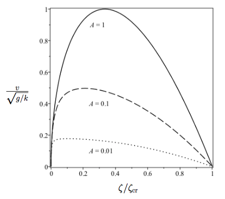
Figure 1: Bubble tip velocity as a function of curvature for various Atwood numbers

At $N=1$, the solution with maximum growth rate is a curved bubble, having a curvature which depends on the Atwood number. The curvature $\sigma_{\rm max}$ which maximizes the velocity satisfies

$$\sigma_{\rm max}^{4}+\frac{1}{A}\sigma_{\rm max}^{3}+\frac{9}{32}\sigma_{\rm max}^{2}-\left(\frac{3}{16}\right)^{3}=0$$

and the corresponding maximum velocity is

$$v_{\rm max}(t)=\left(\frac{1}{k\tau}\right)\left(\frac{t}{\tau}\right)^{\frac{a}{2}}(8\sigma_{\rm max})^{\frac{3}{2}}.$$ (17)

This is a universal relation between the curvature and the maximum velocity.

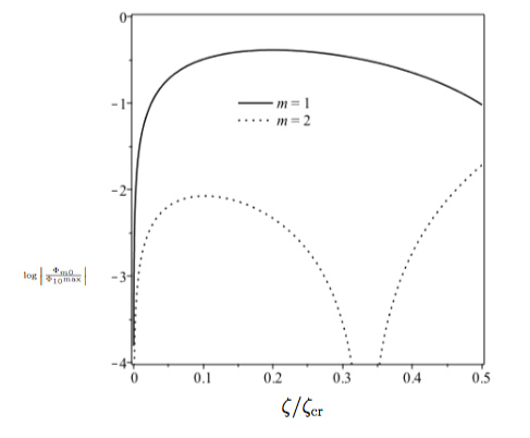
Figure 2: Logarithm of absolute values of the $1^{\rm st}$ (solid line) and $2^{\rm nd}$ (dashed line) Fourier amplitiudes in the heavy fluid

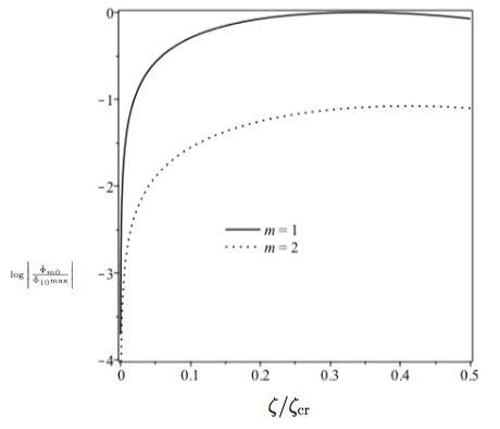
Figure 3: Logarithm of absolute values of the $1^{\rm st}$ (solid line) and $2^{\rm nd}$ (dashed line) Fourier amplitiudes in the light fluid

III.3 The effect of shear

The multiplicity of these solutions is also due to the presence of shear at the interface. We define shear function $\Gamma$ to be the spatial derivative of the jump in the tangential velocity across the interface. We find that in the vicinity of the bubble tip it is $\Gamma=\tilde{M}_{1}-M_{1}$. Specifically,

$$\Gamma(t)=\frac{6kv(t)}{9-64\sigma^{2}}=\frac{6}{\tau}\sqrt{\frac{2A\sigma}{64A\sigma^{2}+9A+48\sigma}}\left(\frac{t}{\tau}\right)^{\frac{a}{2}}$$ (18)

and is a strictly monotone function of $\sigma$, rising from $\Gamma=0$ at $\sigma=0$ to $\Gamma=\Gamma_{\rm max}$ at $\sigma=\sigma_{\rm cr}$. Fig. 4 shows the interface shear as a function of the bubble curvature. We note that the shear function is larger for larger values of the Atwood number $A$, and in each case tends towards a constant value as the curvature increases. Fig. 5 shows the variation of the bubble tip velocity with the interface shear function. We note that the velocity achieves a maximum at some point and that this peak occurs at higher values of the shear function for larger Atwood numbers. The peak velocity itself is also larger for larger Atwood numbers. We particularly note that very soon after the velocity curve reaches its peak, it drops sharply. This rapid change presents significant problems for numerical simulations of RTI.

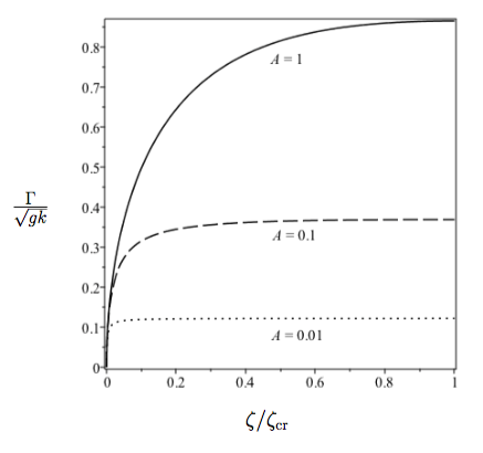
Figure 4: Shear as a function of curvature for various Atwood numbers

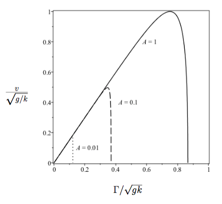
Figure 5: Bubble tip velocity as a function of shear for various Atwood numbers

III.4 Special solutions

III.4.1 The flat bubble

The solution corresponding to a flat bubble is simply $\sigma_{f}=0$, $v_{f}=0$, $\Gamma_{f}=0$, $\Phi_{10{\rm f}}=0$, $\Phi_{20{\rm f}}=0$, $\tilde{\Phi}_{10{\rm f}}=0$, $\tilde{\Phi}_{20{\rm f}}=0$.

III.4.2 The Atwood bubble

The fastest member of the family we refer to as the ‘Atwood bubble’ to emphasise its complex dependence on the Atwood number. The solution is

$$\sigma_{\rm A}=\sigma_{\rm max},\hskip 21.33955ptv_{\rm A}=v_{\rm max}(t),\hskip 21.33955pt\hat{\Gamma}_{\rm A}=\frac{6V_{\rm A}}{9-{V_{\rm A}}^{\frac{4}{3}}},$$ (19)

where

$$V_{\rm A}=k\tau\left(\frac{\tau}{t}\right)^{-\frac{a}{2}}v_{\rm A}(t),\hskip 28.45274pt\hat{\Gamma}_{\rm A}=\tau\left(\frac{\tau}{t}\right)^{-\frac{a}{2}}\Gamma_{\rm A}(t),$$

and the Fourier amplitudes are given by Eq. 16. We note that the $\hat{\Gamma}_{\rm A}(V_{\rm A})$ function is very nearly linear for $V_{\rm A}\in(0,1)$.

In the limit $A\to 1$, the solution is

$$\sigma_{\rm A1}=\frac{1}{8}-\frac{1-A}{64},\hskip 28.45274ptv_{\rm A1}=\frac{1}{k\tau}\left(1-\frac{3-3A}{16}\right)\left(\frac{t}{\tau}\right)^{\frac{a}{2}},$$

$$\Gamma_{\rm A1}=\frac{3}{4\tau}\left(1-\frac{7-7A}{32}\right)\left(\frac{t}{\tau}\right)^{\frac{a}{2}}$$ (20)

and the Fourier amplitudes $\Phi_{10{\rm A1}}$, $\Phi_{20{\rm A1}}$, $\Phi_{10{\rm A1}}$, $\tilde{\Phi}_{20{\rm A1}}$ are, respectively,

$$\frac{1}{k\tau}\left(-\frac{1}{2}+\frac{1-A}{16},\frac{1-A}{32},\frac{3}{4}-\frac{19-19A}{128},-\frac{1}{4}+\frac{7-7A}{128}\right)\left(\frac{t}{\tau}\right)^{\frac{a}{2}}.$$

In the limit $A\to 0$, the solution is

$$\sigma_{\rm A0}=\frac{3}{16}A^{\frac{1}{3}},\hskip 14.22636ptv_{\rm A0}=\frac{1}{k\tau}\sqrt{\frac{27A}{8}}\left(\frac{t}{\tau}\right)^{\frac{a}{2}},\hskip 14.22636pt\Gamma_{\rm A0}=\frac{2k}{3}v_{\rm A}.$$ (21)

and the Fourier amplitudes are $\Phi_{10{\rm A0}}=-\frac{2}{3}v_{\rm A0}$, $\Phi_{20{\rm A0}}=\frac{1}{6}v_{\rm A0}$, $\tilde{\Phi}_{10{\rm A0}}=\frac{2}{3}v_{\rm A0}$ and $\tilde{\Phi}_{20{\rm A0}}=-\frac{1}{6}v_{\rm A0}$.

III.4.3 The ‘Taylor’ bubble

We refer to this bubble as a ‘Taylor bubble’ since its curvature is as in Davies and Taylor (1950) except for a difference in the wavenumber value. The solution is

$$\sigma_{\rm T}=\frac{1}{8},\hskip 28.45274ptv_{\rm T}=\frac{1}{k\tau}\sqrt{\frac{8A}{5A+3}}\left(\frac{t}{\tau}\right)^{\frac{a}{2}},\hskip 28.45274pt\Gamma_{\rm T}=\frac{3k}{4}v_{T}.$$ (22)

The corresponding Fourier amplitudes are $\Phi_{10{\rm T}}=-\frac{1}{2}v_{\rm T}$, $\Phi_{20{\rm T}}=0$, $\tilde{\Phi}_{10{\rm T}}=\frac{3}{4}v_{\rm T}$ and $\tilde{\Phi}_{20{\rm T}}=-\frac{1}{4}v_{\rm T}$. Note that $\Phi_{20{\rm T}}\neq 0$ for $n>1$.

III.4.4 The critical bubble

The solution is

$$\sigma_{\rm cr}=\frac{3}{8},\hskip 14.22636ptv_{\rm cr}=0,\hskip 14.22636pt\Gamma_{\rm cr}=\Gamma_{\rm max}=\frac{1}{\tau}\sqrt{\frac{3A}{2(A+1)}}\left(\frac{t}{\tau}\right)^{\frac{a}{2}}.$$ (23)

and Fourier amplitudes are $\Phi_{10{\rm cr}}=\frac{\Gamma_{\rm max}}{k}$, $\Phi_{20{\rm cr}}=-\frac{\Gamma_{\rm max}}{k}$, $\tilde{\Phi}_{10{\rm cr}}=0$, $\tilde{\Phi}_{20{\rm cr}}=0$.

III.5 Stability

Fig 6 shows stability profiles for various Atwood numbers and $a>0$. We see that the flat bubble is unstable, having $\sigma=\pm\sqrt{AkG}$. In the limits $A\to 1^{-}$ and $A\to 0$ stability is achieved when the curvature reaches

$$\sigma_{\rm st1}=\frac{1}{24}-\frac{1-A}{250},\quad\sigma_{\rm st0}=\frac{-9A+3\sqrt{25A^{2}+8A}}{64(2A+1)}\sim\frac{3\sqrt{2}}{32}\sqrt{A},$$ (24)

respectively. All bubbles are stable for $A\geq\frac{1}{24}$ and hence the Taylor and critcal bubbles are stable. The Atwood bubble is stable when $A=1$, having $\sigma=-\frac{4}{3}\sqrt{kG},-2\sqrt{kG}$. The Atwood bubble for $A=0.1$ and $A=0.01$ are also stable and it would appear that the Atwood bubble is stable for any value of Atwood number $A$ at $N=1$. The $N>1$ analysis is to be presented elsewhere. As is the case for $a=0$, we expect that the stability interval will narrow sharply for $N>1$.

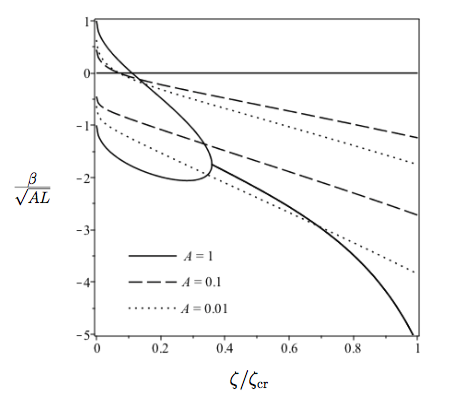
Figure 6: Stability profiles for various Atwood numbers and $a>0$

When $a=0$ and $0\ll A\leq 1$, velocities $v_{\rm A}$ and $v_{\rm T}$ are close to that of the so-called Layzer-type bubble $v_{L}=\frac{1}{k\tau}\sqrt{\frac{2A}{1+A}}$, with which experiments and simulations are often usually compared Anisimov et al. (2013); Abarzhi (2010, 2008); Inogamov (1992); Abarzhi (1998); Abarzhi SI (2006); Layzer (1955); Alon et al. (1995). Thus, our results excellently agree with existing observations Meshkov (1969, 2013); Robey et al. (2003); Kadau et al. (2010); Glimm et al. (2013); Youngs (2013); Abarzhi (2018). Our theory is focused on large-scale dynamics and presumes that interfacial vortical structures are small-scale. This assumption is applicable for fluids very different densities and with finite density ratios. For fluids with very similar densities $0\approx A\ll 1$ other approaches can be employed Anisimov et al. (2013); Abarzhi (2010, 2008, 1998); Abarzhi SI (2006); Abarzhi (2018).

III.6 The velocity field

By accurately accounting for the interplay of harmonics and systematically connecting the interfacial velocity and shear for a broad range of acceleration parameters, we have found that RT dynamics is essentially interfacial: It has intense fluid motion in the vicinity of the interface, effectively no motion away from the interface and shear-driven vortical structures at the interface. The velocity is potentisl in the bulk of each fluid. This velocity pattern is observed in experiments and simulations, demonstrating excellent agreement with our results Meshkov (1969, 2013); Robey et al. (2003); Kadau et al. (2010); Glimm et al. (2013); Youngs (2013); Abarzhi (2018).

IV Discussion

We have found solutions for acceleration driven RTI in a 3D spatially extended periodic flow in both the early-time regime and later-timer regime. In the early-time regime the dynamics is faster than exponential for $a>0$ and slower than exponential for $-2<a<0$. In the later-time regime, bubbles are accelerated for $a>0$, steady at $a=0$, and decelerated for $-2<a<0$. Since the dependencies are given by standard formulae, we can compare various acceleration exponents. The dynamics for small exponents are usually a diagnostic challenge becaue it is slow. Specific examples are fusion, supernovae and nano-fabrication. The dynamics for fast exponents can be easily diagnosed, and the deduced properties can be applied to the slow-dynamics case. Hence we have obtained an important practical result.

The nonlinear bubble velocity and shear, when rescaled as $k\tau(t/\tau)^{-a/2}v$ and $\tau(t/\tau)^{-a/2}\Gamma$, depend only on the interface morphology and flow symmetry. Hence, by analyzing properties of RT bubbles for fast dynamics and large exponents $a>0$, we can obtain properties of those for slow dynamics and small exponents $-2<a<0$ . These are especially convenient for studies of RTI in high energy density plasmas in astrophysics and fusion, where RTI is driven by an explosion or an implosion with blast wave acceleration exponents $-2<a<-1$ in these cases Sedov (1993); Abarzhi (2018); et al (2015).

Our analysis also elaborates upon diagnostic quantities which have not been discussed before. These are the velocity and pressure fields, the interface morphology and bubble curvature, the interfacial shear and its link to the bubble velocity and curvature, the spectral properties of the velocity and pressure, along with the interface growth and growth-rate. By determining the dependence of these quantities on the density ratio, flow symmetry, and acceleration exponent and strength, and by identifying their universal properties, and comparing all of these to data obtained for real fluids, we can further advance our knowledge of RT dynamics in realistic environments, thereby achieving a better understanding of RT relevant processes and also improve methods of numerical modeling and experimental diagnostics of interfacial dynamics in fluids, plasmas and other materials.

Our techniques can also be used to study Richtmyer-Meshkov instability (that is, $a<-2$). The results obtained are very different from those of the Rayleigh-Taylor instability (that is, $a>-2$).

We note also that the expressions obtained in the constant acceleration $a=0$ case are unexpectedly very similar in form to those of the $-2<a<0$ case.

V References

References

- Rayleigh (1883) L. Rayleigh, Proc London Math Soc 14, 170 (1883).
- Davies and Taylor (1950) R. Davies and G. Taylor, Proc R Soc A 200, 375 (1950).
- Landau and Lifshitz (1987) L. Landau and E. Lifshitz, Course of Theoretical Physics (Pergamon Press, New York, 1987).
- Abarzhi et al. (2013) S. Abarzhi, S. Gauthier, and K. Sreenivasan, Turbulent mixing and beyond: non-equilibrium processes from atomistic to astrophysical scales. I & II (Royal Society Publishing, 2013).
- Anisimov et al. (2013) S. Anisimov, R. Drake, S. Gauthier, E. Meshkov, and S. Abarzhi, Phil Trans R Soc A 371, 20130266 (2013).
- Abarzhi (2010) S. Abarzhi, Phil Trans R Soc A 368, 1809 (2010).
- Abarzhi (2008) S. Abarzhi, Physica Scripta T132, 014012 (2008).
- Meshkov (1969) E. Meshkov, Sov Fluid Dyn 4, 101 (1969).
- Meshkov (2013) E. Meshkov, Phil Trans R Soc A 371, 20120288 (2013).
- Robey et al. (2003) H. Robey, Y. Zhou, A. Buckingham, P. Keiter, B. Remington, and R. Drake, Phys. Plasmas 10, 614 (2003).
- Kadau et al. (2010) K. Kadau, J. Barber, T. Germann, B. Holian, and B. Alder, Phil Trans R Soc A 368, 1547 (2010).
- Glimm et al. (2013) J. Glimm, D. Sharp, T. Kaman, and H. Lim, Phil Trans R Soc A 371, 20120183 (2013).
- Youngs (2013) D. Youngs, Phil Trans R Soc A 371, 20120173 (2013).
- Chandrasekhar (1961) S. Chandrasekhar, Hydrodynamic and Hydromagnetic Stability (Oxford University Press, 1961).
- Kull (1991) H. Kull, Phys Rep 206, 197 (1991).
- Gauthier and Creurer (2010) S. Gauthier and B. L. Creurer, Phil Trans R Soc A 368, 368:1681 (2010).
- Nishihara et al. (2010) K. Nishihara, J. Wouchuk, C. Matsuoka, R. Ishizaki, and V. Zhakhovsky, Phil Trans R Soc A 368, 1769 (2010).
- Garabedian (1957) P. Garabedian, Proc R Soc A 241, 423 (1957).
- Inogamov (1992) N. Inogamov, JETP Lett 55, 521 (1992).
- Abarzhi (1998) S. Abarzhi, Phys Rev Lett 81, 337 (1998).
- Abarzhi SI (2006) R. R. Abarzhi SI, Nishihara K, Phys Rev E 73, 036310 (2006).
- Abarzhi (2018) S. Abarzhi, Proc Natl Acad Sci USA , 201714502 (2018).
- Sedov (1993) L. Sedov, Similarity and dimensional methods in mechanics (CRC Press, 1993).
- Arnett (1996) D. Arnett, Supernovae and Nucleosynthesis: An Investigation of the History of Matter, from the Big Bang to the Present (Princeton University Press, 1996).
- Haan (2011) S. Haan, Phys. Plasmas 18, 051001 (2011).
- Peters (2000) N. Peters, Turbulent Combustion (Cambridge University Press, 2000).
- Rana and Herrmann (2011) S. Rana and M. Herrmann, Phys Fluids 23, 091109 (2011).
- Buehler et al. (2007) M. Buehler, H. Tang, A. van Duin, and W. Goddard, Phys Rev Lett 99, 165502 (2007).
- et al (2015) N. S. et al, Phys. Plasmas 22, 102707 (2015).
- Layzer (1955) D. Layzer, Astrophys J 122, 1 (1955).
- Alon et al. (1995) U. Alon, J. Hecht, D. Offer, and D. Shvarts, Phys Rev Lett 74, 534 (1995).